A Turvey-Shapley Value Method for Distribution Network Cost Allocation

Abstract

This paper proposes a novel cost-reflective and computationally efficient method for allocating distribution network costs to residential customers. First, the method estimates the growth in peak demand with a 50% probability of exceedance (50POE) and the associated network augmentation costs using a probabilistic long-run marginal cost computation based on the Turvey perturbation method. Second, it allocates these costs to customers on a cost-causal basis using the Shapley value solution concept. To overcome the intractability of the exact Shapley value computation for real-world applications, we implement a fast, scalable and efficient clustering technique based on customers’ peak demand contribution, which drastically reduces the Shapley value computation time. Using customer load traces from an Australian smart grid trial (Solar Home Electricity Data), we demonstrate the efficacy of our method by comparing it with established energy- and peak demand-based cost allocation approaches.

I Introduction

The rapid rise in the penetration levels of distributed energy resources in low-voltage distribution networks necessitates the design of network tariffs that allocate associated network costs in an efficient, fair and equitable manner to network users. Hence, distribution network service providers (DNSPs) and regulators in most jurisdictions are challenged with the tasks of designing efficient tariffs that are reflective of network cost drivers [1]. Recent studies in this area have explored different methods for distribution network pricing, including transmission network pricing methodologies, such as Locational Marginal Pricing (LMP), Postage Stamp (PS), MW-Mile, MVA-Mile, Average Participation (AP), and Marginal Participation (MP) [2, 3, 4, 5, 6], Ramsey-Boiteux pricing, cooperative game theory or other extemporaneous cost allocation methodologies. However, in order to establish the performance of these methods with respect to established tariff design principles [7], which includes cost reflectiveness, efficiency, stability and fairness, we need to define a measure (benchmark) of overall performance, with which to compare existing methods. To this end, the purpose of our study is to use a principled cost allocation method as a performance benchmark for other allocation methodologies.

Distribution network costs typically comprises three major cost components–energy costs, long-run marginal cost (LRMC), and residual (such as retail charges) costs. In order to adequately recover these cost components, network tariffs should be structured such that the fixed, energy and/or demand charges efficiently send the right price signals to customers to respond appropriately. For example, [8] used a three-part tariff for distribution network cost allocation. Here, the residual costs ($/day) were recovered through Ramsey pricing, while the LRMC ($/kW) and energy costs ($/kWh) were recovered through coincident peak pricing and distribution locational marginal pricing (DLMP) respectively.

Nevertheless, network tariffs historically only consisted of energy-based (volumetric) and residual charges due to two reasons: (i) there was little need to signal the LRMCs because loads per feeder were relatively flat and (ii) pricing mechanisms available to utilities were severely constrained by metering technology. However, with the introduction of smart meters, it is possible to implement tariffs which reflect congestion costs that drives network investments. As such, network tariffs should be based on customers demand at network peak [9, 10, 11, 12, 8, 13]. It should be time- and location-specific and should account for network losses and actual customer energy use. Additionally, a fair and equitable tariff should also eliminate or reduce inter-customer subsidies created due to PV owners, while safeguarding vulnerable customers [14, 15].

Unlike volumetric tariffs, peak demand-based tariffs are robust to technological changes (such as solar PV, EV or battery storage) which reshapes customers’ demand profiles while effectively signalling peak demand costs to customers [15, 16]. Thus, residual and/or LRMC costs can be recovered partly through demand-charges instead of constantly increasing fixed or energy charges for all customers [6, 17]. So far, coincident peak pricing (CPP) and critical peak pricing have been proposed to mitigate the impacts of DER on the equity of network cost allocations. Although peak demand-based tariffs are more complex than energy-based tariffs, they can better allocate network costs on a cost-causal basis and ensure a stable revenue for network companies [15, 17]. Furthermore, [18] showed that customer bill volatility reduces with demand-based tariffs compared to real time pricing and time-of-use tariffs. Contrarily, [12] tested demand-based tariffs proposed by the Australian Energy Regulator (AER) on households in Sydney. It was concluded that without due adjustments made, these tariffs are low in cost-reflectivity. Generally, the suitability of network tariffs in terms of fairness and cost-reflectivity depends on the assumptions made in the tariff design and on customers’ price response [19]. This further highlights the need for a principled cost allocation benchmark.

Further still, the distribution network tariff design problem encompasses more than the aforementioned requirements. Beyond these, there are other three salient tariff design questions that need to be answered in order to achieve a cost-reflective pricing and appropriate customer response: (i) What LRMC calculation method should be used – the Turvey perturbation method or the Average Incremental Cost method? (ii) What peak demand should be the basis for charging customers – individual customer peak, distribution network coincident peak or zone-substation peak? and, (iii) What is the optimal frequency of peak demand measurement – monthly or yearly basis? [17]. The answers to these questions form the basis for practically implementing tariffs that better recuperate forward-looking network costs. However, there are no clear-cut answers to these questions, because choices for network companies depend on other factors, such as customer socio-demographics, customer class, and the availability of smart meters and energy management systems. Nonetheless, recent research in the area argues that demand-based tariffs should be based on network coincident peak since it better signals LRMC. However, in practice, customers’ coincident peak demand is hard to measure and thus CPP is difficult to implement. Thus, demand charges are a step-forward to attaining optimal network tariffs.

In this paper, we seek, based on established economic principles, to make a further step towards the design of equitable network pricing. Our focus is to provide a measure for the fair and efficient allocation of costs that signal the drivers of future network investment. To achieve this, we develop a novel method to apportion the LRMC, using a probabilistic approach to the Turvey perturbation method ([20]) linked via the characteristic function of a cooperative game to the Shapley value (SV) cost allocation rule [21, 22].

In more detail, the Turvey perturbation method is a forward-looking and more time- and location-specific method for LRMC estimation, compared to the simpler average incremental cost methods widely used by network companies [17]. Furthermore, [23, 24] argue that the Turvey perturbation method is the preferred option since it better aligns with the underpinning principles governing LRMC. However, research in [25] concluded that both methods can be equally used for LRMC calculations.

At the same time, the SV gives a vector-valued solution to a cooperative transferable utility (TU) game, where the total cost or worth of a coalition is defined by a single-valued characteristic function. In our method, the characteristic function is the probabilistic LRMC defined using the Turvey perturbation method. The SV has found several applications including consumer demand response compensation [26, 27, 28], transmission network cost allocation [29, 30, 31], distribution network loss allocation [32], and other cost allocation problems [33, 34, 35, 26, 27]. However, due to the computational complexity of computing the exact SV for a large number of players, it’s application is usually limited to small problems. Recent research in this area, nonetheless, has seen developments of approximate methods of calculating the SV in polynomial time [36, 37, 34, 38, 39, 35, 27]. In [27], a comparison of the accuracy and scalability of two approximate SV computation algorithms was made, namely linear-time approximation [36] and stratified sampling [39, 40] techniques. While the stratified sampling approach was more accurate, the linear-time approximation required less memory and computation time as the number of players increased. This is a general finding, so with these methods, there is always a trade-off between accuracy and computational complexity. Moreover, some of these methods are only suited to weighted voting games, which does not match our cost-allocation problem. In a different research direction, a clustering approach was adopted in [38], where customers are segmented into major classes. However, customers in the same class are assigned the same SV. Conversely, for distribution network cost allocation, this is not the case, as the SV should be different for all customers.

In light of these shortcomings, we derive a computationally-efficient clustering algorithm, to allocate network costs based on the Turvey-Shapley value method. The SV is computed at the level of clusters, and individual customers are allotted a portion of this SV based on their average coincident peak demand contribution to each coalition of their representative cluster. This approximation approach is validated by comparison to the exact SV calculation, for which the SV estimation error is shown to be small and reduces as the number of customers increases (i.e. when approximation become computationally necessary). Furthermore, as the SV method best allocates network costs in a principled, fair and stable manner, we used it as a benchmark to measure the cost-reflectivity of other cost allocation methodologies. In summary, the analysis in this paper extends the preliminary results in our earlier conference paper [41] in the following ways:

• We propose a probabilistic approach to the Turvey LRMC computation via a Weibull distribution, which gives an unbiased estimate of forward-looking network costs.

• We propose a peak load contribution clustering technique interleaved with the Turvey-Shapley value method to compute the Shapley value for large number of customers with low computation time and estimation error.

• We demonstrate the effectiveness of our methodology using real customer load traces from the Solar Home Electricity Data. Our results show that the proposed allocation method is the most reflective of network capacity costs compared to other cost allocation methodologies.

The remainder of this paper is structured as follows. Section II provides preliminaries on cooperative game theory and the Shapley value. In Section III, we describe the methodology, including the Turvey pricing method. The results are presented and discussed in Section IV. Section V concludes.

II Preliminaries

In this section, we provide a background to cooperative games, the Shapley value and its characteristics, and the Turvey perturbation method.

II-A Cooperative Games

Formally, we consider the class of transferable utility (TU) games, which are cooperative games that allow the transfer of worths between players. If the players in a cooperative game agree to work together, they form a coalition. If all $n$ players form a coalition, it is called the grand coalition. Each player incurs some private cost in completing its component of the joint action, while collectively, the joint action has some worth associated with it.

Definition II.1.

A TU game is given by $\Gamma=\langle\mathcal{N},w\rangle$ where:

• $\mathcal{N}$ is a set of $n$ players, and

• $w(\mathcal{S})$ is a characteristic function, $w:2^{n}\to\Re_{+}$ with $w(\emptyset)=0$, that maps from each possible coalition $\mathcal{S}\subseteq\mathcal{N}$ to the worth of $\mathcal{S}$.

Before defining the Shapley value, we first formally define some important characteristics of any solution to a TU game.

Definition II.2.

Given a $\Gamma$, a solution concept defines a worth to each player, which is a vector of transfers (worths), $\phi=(\phi_{1},\ldots,\phi_{i},\ldots,\phi_{n})\in\Re^{n}$.

We denote the sum of worths as $\sum_{i\in\mathcal{S}}\phi_{i}=\phi(\mathcal{S})$. Some desirable properties of solutions concepts include the following; a solution is:

• Efficient if $\phi(\mathcal{S})=w(\mathcal{S})$, so that the worth vector exactly divides the coalitions worth,

• Symmetric if $\phi_{i}=\phi_{j}$ if $w(\mathcal{S}\cup\{i\})=w(\mathcal{S}\cup\{j\}),\ \forall~{}\mathcal{S}\subseteq N\setminus\{i,j\}$. This means that equal worths are made to symmetric players, where symmetry means that we can exchange one player for the other in any coalition that contains only one of the players and not change the coalition’s worth.

• Additive if for any two additive games the solution can be given by $\phi_{i}(v_{1}+v_{2})=\phi_{i}(v_{1})+\phi_{i}(v_{2})$ for all players. That is, an additive solution assigns worths to the players in the combined game that are the sum of their worths in the two individual games.

• Zero worth to a null player if a player $i$ that contributes nothing to any coalition, such that $w(\mathcal{S}\cup\{i\})=w(\mathcal{S})$ for all $\mathcal{S}$, then the player receives a worth of 0.

II-B The Shapley Value (SV)

Solution concepts in cooperative game theory define divisions of the group reward among players, while considering the rewards available to each alternative coalition of players. The SV is one of such solution concepts which also satisfies the desirable properties listed above, by virtue of its definition.

Definition II.3.

The SV allocates to player $i$ in a coalitional game $\langle w,\mathcal{N}\rangle$ the worth:

$$\phi_{i}(w)=\frac{1}{n}\sum_{\mathcal{S}\subseteq\mathcal{N}\setminus i}\binom{n-1}{|\mathcal{S}|}^{-1}\left(w(\mathcal{S}\cup\{i\})-w(\mathcal{S})\right)$$ (1)

Here, the vector-valued function $\phi$ has the following intuitive interpretation: consider a coalition being formed by adding one player at a time. When $i$ joins the coalition $\mathcal{S}$, its marginal worth is given by $w(\mathcal{S}\cup\{i\})-w(\mathcal{S})$. Then, for each player, its SV worth is the average of its marginal contributions over the possible different orders in which the coalition can be formed.

The expression in (1) can also be interpreted as a player’s contribution to all subsets of $\mathcal{N}$ that do not contain it, where the binomial term is the number of coalitions of size $|\mathcal{S}|$. We can further expand this expression to identify a useful approximation. Specifically, the summation in (1) can be expressed in terms of the size of the coalitions that $i$ is added to, as follows:

$$\phi_{i}(w)=\frac{1}{n}\sum_{k=0}^{n-1}\left(\binom{n-1}{k}^{-1}\sum_{\mathcal{S}\in\mathcal{S}^{k}}\left(w(\mathcal{S}\cup\{i\})-w(\mathcal{S})\right)\right)$$ (2)

where: $\mathcal{S}^{k}=\{\mathcal{S}\subseteq\mathcal{N}\setminus i\,:\,|\mathcal{S}|=k\}$ is the set of coalitions of size $k$ that exclude $i$. We can now approach the SV by approximating the inner term for each size $k\in\{0,\ldots,n-1\}$.

One approach is to statistically estimate the term:

$$\chi^{k}=\binom{n-1}{k}^{-1}\sum_{\mathcal{S}\in\mathcal{S}^{k}}\left(w(\mathcal{S}\cup\{i\})-w(\mathcal{S})\right)$$ (3)

using a sample-based approach. This is a randomised sampling algorithm described in detail in Section III-C.

Algorithm 1 Exact Turvey-Shapley Value Algorithm (Exact)

$\mathcal{N}$: set of players/customers, $\mathcal{N}=\{1,..,n\}$
$\mathcal{L}$: set of all coalitions, $\mathcal{L}=\{\mathcal{S}^{1},..,\mathcal{S}^{l},...,\mathcal{S}^{2^{n}-1}$}

1:for each customer $i\in\mathcal{N}$ do

2:    for each coalition $\mathcal{S}\in\mathcal{L}:i\in\mathcal{S}$ do

3:         $\mu$ = 50POE yearly peak demand of $\mathcal{S}$

4:         Find $X\sim\mathcal{W}(\alpha,\beta)$ of $\mu$ exceeding line limit $x$

5:         $\alpha=\mu/\Gamma(1+1/\beta)$ with $\beta=1.5$

6:         if $P(X\geq x)<0.001$ then

7:             $w(\mathcal{S})=P(X\geq x)Y$

8:         else

9:             $w(\mathcal{S})=0$

10:         end if

11:         Compute $M_{\mathcal{S}_{i}}=w(\mathcal{S})-w(\mathcal{S}-\{i\})$

12:         Compute $K_{\mathcal{S}_{i}}=(1/n!)(|\mathcal{S}|-1)!\;(n-|\mathcal{S}|)!$

13:    end for

14:    Return SV of $i$, $\phi_{i}(w)=\sum_{\begin{subarray}{c}\mathcal{S}\in\mathcal{L}\end{subarray}}K_{\mathcal{S}_{i}}M_{\mathcal{S}_{i}}$

15:end for

II-C The Turvey Perturbation Method

The Turvey perturbation method [20] is one technique used to estimate the LRMC of capacity-based investments. It quantifies the effects of a (small) permanent change in demand $Q$ on future capital costs $C$. It is defined in [25] as:

$$\textrm{Turvey LRMC}=\frac{PV(\Delta C)}{PV(\Delta Q)}$$ (4)

The expression in (4) translates to–the ratio of the present value of change in costs (due to a permanent change in demand) to the present value of the permanent change in demand. The Turvey perturbation method therefore involves forecasting demand over the estimation period, with a certain confidence level. For this, we assume a small growth in yearly peak demand with a 50% probability of exceedance.

As explained in detail in the next section, in our methodology, the probability that this value exceeds the network line limit informs the LRMC. This probabilistic approach to the Turvey perturbation method, achieved via a Weibull distribution, is used to construct the characteristic function for the SV computation.

III Methodology

In this section, we detail the steps taken to assess the cost-reflectivity in the allocation of distribution network tariffs to LV residential customers, with the SV allocation being the benchmark. First, we explain the Turvey-Shapley value LRMC estimation and allocation methodology. Second, we describe algorithms to determine the exact SV for a set of customers $\mathcal{N}$, and its approximation. The approximation algorithms are required to compute the SV for $n>25$ players, with lower computational burden and minimal loss in accuracy.

III-A Turvey-Shapley Value LRMC Methodology

The proposed Turvey-Shapley value LRMC methodology involves interleaving of a novel probabilistic approach to the Turvey perturbation method with the SV characteristic function, and is illustrated in Algorithm 1. In this section, we explain the steps for the Turvey LRMC estimation and SV cost allocation.

First, we calculate the line limit $x$ of the given network with line augmentation cost $Y$. This is given as the yearly peak demand of the network (i.e. grand coalition of customers) multiplied by a factor of 1.5 (to account for distribution line emergency limit). We have assumed that the probability of a coalition’s 50 POE peak demand exceeding the line limit follows a Weibull distribution, $X\sim\mathcal{W}(\alpha,\beta)$. The two-parameter Weibull distribution function is defined as:

$$F_{\alpha,\beta}(x)=1-\exp\Big{[}-\Big{(}\frac{x}{\alpha}\Big{)}^{\beta}\Big{]}\quad\mathrm{for}\quad x\geq 0$$ (5)

where $\alpha>0$ is the scale parameter and $\beta>0$ is the shape parameter. In order to obtain the standard fat-tailed Weibull distribution that is required in this study, $\beta$ is taken as 1.5.

Then, for each coalition, we assume a yearly peak demand growth rate of 1% as the 50 POE value, which is taken as the mean $\mu$ of the Weibull distribution. Given the mean and shape factor, we calculate the scale factor of the distribution. If the tail probability $P(X\geq x)$ of a coalition’s 50 POE peak demand exceeding the line limit is less than 0.001, we neglect the coalition cost (set as zero) in the incremental cost (IC) calculations for a particular customer in each coalition size. For example, if $Y$ is $1M, then we neglect coalitions with cost less than $1k, which improves the incremental cost computation time of each customer. Otherwise, the coalition cost is given as $P(X\geq x)Y$, that is, the coalition’s expected LRMC under the corresponding Weibull distribution. The SV for each customer $i\in\mathcal{N}$ is calculated as the average of its marginal contributions to all coalitions containing $i$, as in (1).

In the next three subsections, we describe the exact SV algorithm (Exact), and two algorithms (Sampling and Clustering) to compute the approximate SV for up to 25 customers.

III-B Direct Enumeration

The exact algorithm (Exact), also known as direct enumeration, is based on (1) and is described in Algorithm 1. In terms of computational speed, it performs well with $n<20$ players. But with $n>25$, its performance (w.r.t. speed and memory requirements) deteriorates because of the time taken and memory required to compute the large ($2^{n}-1$) $\times$ $n$ coalition matrix. Note that Line 2 in Algorithm 1 can be broken down into $n$ coalition sizes according to (2).

III-C Randomised Sampling

As explained in Section II-B, we use a sample-based randomised algorithm which statistically estimates (3), to provide approximate SV calculations based on (2). With this, we do not perform all the incremental cost calculations ($2^{n-1}$) required to compute the exact SV for each customer. Instead, we do this only for coalition sets that contain more than 10,000 possible coalitions of the same size. In Algorithm 2 (Sampling), we first select randomly a pilot sample ($|\mathcal{P}|=K$) from such large coalitions, where $K$ is determined by trial and error. Then, the standard deviation $\sigma_{\mathcal{P}}$ of the marginal contribution of customer $i$ to the sampled coalition is computed, followed by the calculation of the optimal sample size using:

$$|\mathcal{P}^{\prime}|=\Big{(}\frac{Z\sigma_{\mathcal{P}}}{d}\Big{)}^{2}$$ (6)

where $Z=1.96$ is the z-score of 95% confidence in a Gaussian distribution and $d=0.2$ is taken to be the margin of error for the sampling estimation.

Algorithm 2 Randomised Sampling Algorithm (Sampling)

$\mathcal{N}$: set of players/customers, $\mathcal{N}=\{1,...,n\}$
$\mathcal{K}$: partition of set of $k$-sized coalitions, $\mathcal{K}=\{\mathcal{S}^{1},..,\mathcal{S}^{k},..,\mathcal{S}^{n}\}$

1:for each customer $i\in\mathcal{N}$ do

2:    for each set of $k$-sized coalitions $\mathcal{S}^{k}\in\mathcal{K}$ do

3:         Find $\mathcal{G}\subset\mathcal{S}^{k}:\forall\ \mathcal{Z}\in\mathcal{G},i\in\mathcal{Z}$

4:         if $|\mathcal{S}^{k}|<10000$ then

5:             for each coalition $g\in\mathcal{G}$ do

6:                 $\theta_{g}=\frac{(k-1)!\;(n-k)!}{n!}\left(w(g)-w(g-\{i\})\right)$

7:             end for

8:             $\vartheta_{\mathcal{S}^{k}}=\sum_{g\in\mathcal{G}}\theta_{g}$

9:         else

10:             Sample $|\mathcal{P}|$ coalitions from $|\mathcal{G}|:|\mathcal{P}|=K$

11:             for each coalition $p\in\mathcal{P}$ do

12:                 $\theta_{p}=\left(w(p)-w(p-\{i\})\right)$

13:             end for

14:             Compute standard deviation $\sigma_{\mathcal{P}}$ of all $\theta_{p\in\mathcal{P}}$

15:             Compute optimal sample size, $|\mathcal{P}^{\prime}|$ using (6)

16:             Sample $|\mathcal{P}^{\prime}|$ coalitions from $|\mathcal{G}|$

17:             for each coalition $p^{\prime}\in\mathcal{P}^{\prime}$ do

18:                 $\theta_{p^{\prime}}=\frac{(k-1)!\;(n-k)!}{n!}\left(w(p^{\prime})-w(p^{\prime}-\{i\})\right)$

19:             end for

20:             $\vartheta_{\mathcal{S}^{k}}=\sum_{p^{\prime}\in\mathcal{P}^{\prime}}\theta_{p^{\prime}}$

21:         end if

22:    end for

23:    $\phi_{i}=\sum_{\mathcal{S}^{k}\in\mathcal{K}}\vartheta_{\mathcal{S}^{k}}$

24:end for

III-D Clustering Method

The clustering method illustrated in Algorithm 3 is also based on (2). In this method, we first cluster $|\mathcal{H}^{m}|=125$ customers from the Ausgrid Solar Home Electricity Data set into $n=5$ representative load profile clusters (with minimum customer set $|\mathcal{H}^{1}|=25$). Here, end-users are clustered based on their half-hourly average daily consumption pattern for a year using the k-means clustering algorithm. Next, for each set of network users $\mathcal{H}^{h}\in\mathcal{H}$, we find the yearly demand (with 30-minute resolution) of each cluster $i\in\mathcal{N}$, by summing the half-hourly demand of all customers belonging to cluster $i$. Then, we find the average contribution $\boldsymbol{V}_{g}^{\mathcal{H}^{h}_{i}}$ of member customers to the yearly peak demand of cluster $i$ over all coalitions $g\in\mathcal{G}$.

After computing the SV of each cluster, the cluster cost is then apportioned to its member customers according to their contribution. It is worth noting that the algorithm can be scaled to compute the SV for $|\mathcal{H}^{m}|>125$ network users in our dataset, with just an insignificant clustering overhead computation cost for allocating customers into 5 clusters; and moreover, it would scale to settings with up to 25 clusters irrespective of the total number of customers.

.

Algorithm 3 Clustering Algorithm (Clustering)

$\mathcal{H}$: partition of set of network users, $\mathcal{H}:=\{\mathcal{H}^{1},..,\mathcal{H}^{h},..,\mathcal{H}^{m}\}$
$\mathcal{N}$: set of players/clusters, $\mathcal{N}=\{1,...,n\}$
$\mathcal{K}$: partition of set of $k$-sized coalitions, $\mathcal{K}=\{\mathcal{S}^{1},..,\mathcal{S}^{k},..,\mathcal{S}^{n}\}$

1:Cluster $|\mathcal{H}^{m}|$ customers into $n$ clusters

2:for each $\mathcal{H}^{h}\in\mathcal{H}$ do

3:    for $t\longleftarrow 1\ \mathbf{to}\ 100\ \mathbf{step}\ 1$ do$\triangleright$ 100 MC simulations

4:         Sample $|\mathcal{H}^{h}|$ customers uniformly from $|\mathcal{H}^{m}|$

5:         for each cluster $i\in\mathcal{N}$ do

6:             for each set of $k$-sized coalitions $\mathcal{S}^{k}\in\mathcal{K}$ do

7:                 Find $\mathcal{G}\subset\mathcal{S}^{k}:\forall\ \mathcal{Z}\in\mathcal{G},i\in\mathcal{Z}$

8:                 for each coalition $g\in\mathcal{G}$ do

9:                     Find $\mathcal{H}^{h}_{i}\subset\mathcal{H}^{h}$ $\triangleright$ customers in cluster $i$

10:                     $\boldsymbol{V}_{g}^{\mathcal{H}^{h}_{i}}=[v_{g}^{1},...,v_{g}^{|\mathcal{H}^{h}_{i}|}]$ $\triangleright$ cust. contr. to $w(g)$

11:                     $\theta_{g}=\frac{(k-1)!\;(n-k)!}{n!}\left(w(g)-w(g-\{i\})\right)$

12:                 end for

13:                 $\vartheta_{\mathcal{S}^{k}}=\sum_{g\in\mathcal{G}}\theta_{g}$

14:             end for

15:             $\phi_{i}=\sum_{\mathcal{S}^{k}\in\mathcal{K}}\vartheta_{\mathcal{S}^{k}}$ $\triangleright$ SV of cluster $i$

16:             $\boldsymbol{\phi_{t}^{\mathcal{H}^{h}_{i}}}=(\phi_{i}/|\mathcal{G}|)\sum_{g\in\mathcal{G}}\boldsymbol{V}_{g}^{\mathcal{H}^{h}_{i}}$ $\triangleright$ SV–customers in $i$

17:         end for

18:    end for

19:end for

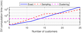
(a)

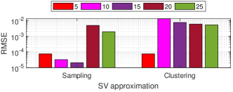
(b)

Figure 1: (a) SV computation time for 5 – 25 customers (b) Error in approximate SV calculation for 5 – 25 customers. For both plots, the y-axis is in log scale.

IV Case Study, Results and discussion

In this section, we assess the computational performance and accuracy of the SV approximation methods, the correlation of SV with three peak demand indicators commonly used to define tariffs, and compare alternative pricing methods with the SV cost allocation.

To begin, we define the following three peak demand indicators as follows:

• Coincident peak demand (CPD): This refers to a customer’s coincident peak demand at the time of the network’s yearly peak load.

• Individual peak demand (IPD): This refers to a customer’s yearly peak demand.

• Total peak demand (TPD): This refers to the sum total of a customer’s monthly peak demand values in a year.

As case study, the net load traces (solar PV and demand) used in this work were sourced from the Ausgrid (DNSP in NSW) Solar Home Electricity Data. The dataset comprises three years of half-hourly resolution smart meter data for the period between July 2010 to June 2013, for 300 residential customers in the Sydney region of Australia. However, we could only extract 125 customers from this dataset with complete solar PV and demand data, for the period between July 2012 to June 2013. This information is used to obtain the above defined peak demand indicators for each customer.

We also employ network tariff data from Ausgrid, given in Table I, which enables us make a rough estimate of the revenue obtained for these customers under the flat and ToU energy network prices.

TABLE I: Network Tariff Data

Tariff Type	Fixed charge $\mathrm{c}\mathrm{/}\mathrm{d}\mathrm{a}\mathrm{y}$	Anytime Energy $\mathrm{c}\mathrm{/}\mathrm{k}\mathrm{W}\mathrm{h}$	Off peak Energy $\mathrm{c}\mathrm{/}\mathrm{k}\mathrm{W}\mathrm{h}$	Shoulder Energy $\mathrm{c}\mathrm{/}\mathrm{k}\mathrm{W}\mathrm{h}$	Peak Energy $\mathrm{c}\mathrm{/}\mathrm{k}\mathrm{W}\mathrm{h}$
Flat	40.097	11.163	-	-	-
ToU	40.097	-	2.805	7.086	27.335

IV-A SV Computation Time and Accuracy

Here, we compare the computational performance and accuracy of the different SV calculation algorithms. For this first set of computations, we have assumed that all customers possess solar PV, so the net load is used to compute their monthly peak demand. Fig. 1a shows the SV computation time in minutes for all customer sizes from 5 up to 25 users. A related point to consider is that the exact SV computation for more than 25 users is not computationally feasible. The Exact algorithm performs best for $n<15$ customers, but with $n\geq 15$, this is not the case. It takes 418 minutes to compute the SV for $n=25$ customers, due to the time and memory consuming coalition matrix generation and the corresponding coalition cost function calculations.

Conversely, there is a significant improvement in computational performance with the first approximate algorithm compared to Exact. Sampling takes only 98 minutes to compute the SV for $n=25$ (about a quarter of the time taken for Exact). This reduction in computation time is as a result of performing IC calculations for a select (optimal) sample, using a constant number as a pilot sampling size, instead of performing the IC calculations for all coalitions (in Exact) at the same time. Furthermore, splitting the total coalitions into $n$ coalition sizes in Sampling overcomes the memory limitations of Exact.

On the other hand, the clustering algorithm takes the least time to compute the SV for $n\geq 15$ customers. This is because the SV calculation is done for only 5 players (or clusters), with a little overhead computation cost for clustering.

To evaluate the accuracy of the sampling and the clustering technique, we find the root mean square error (RMSE) in the SV estimation. Fig. 1b shows RMSE values between $10^{-2}$ and $10^{-5}$ relative to mean values between $0.04$ and $0.2$ for $n\leq 25$ customers. Although the sampling approach is more accurate than the clustering technique for $5<n\leq 25$, it cannot be up-scaled to $n>25$ players, without a significant increase in the computation time. Besides, with the clustering technique, the estimation error reduces as more customers are added to make the clusters more representative.

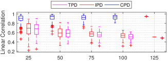
(a) Without PV

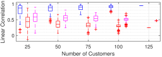
(b) With PV

Figure 2: SV linear correlation coefficient box plot. CPD–coincident peak demand, IPD–individual peak demand, TPD–total peak demand. Note that there is no statistical variance for $n=125$.

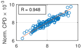
(a)

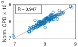
(b)

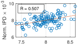
(c)

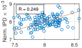
(d)

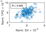
(a) Without PV

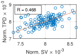
(b) With PV

Figure 3: SV linear correlation scatter plot for 125 customers. CPD–coincident peak demand, IPD–individual peak demand, TPD–total peak demand.

TABLE II: Mean SV correlation with Peak demand Indicators

Scenario	Peak demand Indicator	Customers
		25	50	75	100	125
Without PV	Coincident	0.8773	0.9134	0.9114	0.9272	0.9478
	Individual	0.6668	0.5891	0.5644	0.5321	0.5065
	Total	0.6626	0.5833	0.5541	0.5140	0.4848
With PV	Coincident	0.7967	0.8380	0.8780	0.9098	0.9473
	Individual	0.4113	0.3625	0.3291	0.2918	0.2493
	Total	0.5700	0.5512	0.5277	0.5016	0.4685

IV-B SV Linear Correlation with Peak demand Indicators

This section shows the results obtained by finding the linear correlation between the SV computed using the clustering technique and the peak demand indicators, for two scenarios (i) all customers without PV and (ii) all customers with PV. Since the SV is computed for 100 Monte Carlo runs based on uniform random sampling, the Pearson’s correlation coefficients (R-value) are presented as box plots in Fig. 2 while Table LABEL:sv_corr shows the mean values, for $\mathcal{H}$ of size 25, 50, 75, 100, and 125.

For Scenario 1 (Fig. 2a), the SV correlates more with Individual peak demand than with Total peak demand but for Scenario 2 (Fig. 2b), the converse is the case. It is worth noting that Individual and Total corresponds to charging customers based on their yearly peak load and monthly peak load respectively. Without PV, a customer’s true demand is revealed, which is less sensitive to weather, so individual peak demand dominates. However, with PV, a customer’s demand profile is modified with PV generation which is season-dependent, and as such it’s better to charge customers on a monthly basis. Nevertheless, for both scenarios, the SV correlates most with Coincident peak demand, because it drives augmentation cost the most.

Figs. 3a and 3b show the scatter plot for SV correlation with the peak demand indicators for $n=125$ customers without PV and with PV respectively. For Scenario 1, the mean R-values are 0.948, 0.507 and 0.485, for Coincident, Individual, and Total peak demand respectively while the R-values for Scenario 2 are 0.947, 0.249 and 0.468, for Coincident, Individual, and Total peak demand respectively. While CPD and TPD have similar values in both scenarios, IPD is considerably different. This is because a customer’s (individual) yearly peak demand changes significantly with the addition of PV.

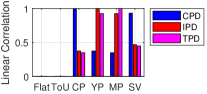
(a)

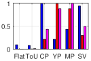
(b)

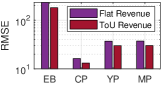
(a) Without PV

   

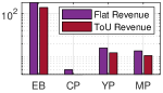
(b) With PV

Figure 4: (a) Correlation between cost allocation method and peak demand variants (top) and error in cost allocation from the SV allocation (bottom). EB–energy-based, CP–coincident peak, YP–yearly peak, MP–monthly peak.

IV-C Comparison of Cost Allocation Methodologies

Here, we evaluate how different energy-based and peak demand-based cost allocation methodologies compare to the SV, by measuring the correlation between normalised customer cost allocation and specifically-defined peak demand indicators. First, we perform the SV computation for $n=125$ customers, for both scenarios. Then, we estimate the revenue obtained by the DNSP for these customers under the two tariffs (Flat- and ToU-based) described in Section III. For this, we have have neglected the feed-in-tariff (FiT) as it is administered through a different mechanism and handled by retailers in the Australian electricity system’s regulatory and billing arrangements. Therefore, we use only the power import from the grid for our calculations.

We consider the following cost allocation methods in our analysis:

• Energy-based (EB - Flat or ToU)

• Coincident peak load (CP - Coincident peak)

• Yearly peak load (YP - Individual peak)

• Monthly peak load (MP - Total peak) and

• Shapley value cost allocation (SV)

In the first method, cost allocation is done according to the revenue calculations under Flat and ToU tariff for $n=125$ customers, using tariff values in Table I. For the rest, we split the total revenue obtained using the energy-based tariffs, according to the normalised SV and the normalised Coincident, Individual, and Total peak demand values for each customer.

The top part of Fig. 4 shows the correlation between the different cost allocation methodologies and the peak demand indicators. From these, we can deduce that the SV provides a fine balance between coincident, individual and aggregate peak demand, since it properly accounts for network usage at times other than the coincident network peak. This is by virtue of the way it is being computed, by evaluating the marginal contribution of customers to all possible coalitions. Although, the major cost driver for distribution networks is the coincident peak demand, it is necessary for a cost-reflective tariff design to appropriately account for aggregate and individual customer peak demand. Furthermore, the yearly and monthly peak demand allocation are also not cost-reflective, since they have a lower correlation with coincident peak demand compared with the SV allocation. Energy-based allocation methods perform worst as they show much lower correlation with the peak demand indicators. However, the results for Scenario 2 show that ToU-energy based allocation is better than that of Flat-energy based allocation as it shows comparatively higher R-values. Moreover, these results implicitly show that inter-customer subsidies will be reduced since customers would be paying their fair share, given the similar R-value for Coincident peak demand in both scenarios.

At the bottom part of Fig. 4, we show the error (RMSE) in actual cost values that will arise when a DNSP allocates cost to customers using less optimal cost allocation methodologies. This translates to inaccurate wealth transfer amongst customers in a distribution network. As expected, there are higher RMSE values resulting from energy-based cost allocation methods. This implies that they are least cost-reflective for both scenarios, both in terms of cost-causality and equity in cost allocation. Also, for both scenarios, the coincident peak load allocation results in the least error because the main cost driver for networks is the coincident peak. While the monthly peak allocation, and the yearly peak demand allocation method results in similar RMSE values for Scenario 1, this is not the case for the second scenario. When all customers possess PV, the monthly peak allocation results in slightly lower RMSE compared to the yearly peak demand allocation. This shows that for residential customers with PV, using a monthly peak demand network tariff is more cost reflective than a yearly peak demand tariff. It will be unfair to charge customers based on their sole highest yearly peak demand, which occurs in just one month of a year, and does not account for the seasonality in energy consumption which comes with PV generation.

V Conclusions and Future Work

In this work, we showed the efficacy of the Turvey-Shapley value method in calculating and apportioning LRMC to network users in a cost-reflective way and with low computational burden using the proposed clustering technique.

We have demonstrated that the SV is a cost-reflective cost allocation method for networks with a large number of customers, regardless of PV adoption. This is because the SV is a principled technique, which provides a proper balance between the peak demand indicators (network cost drivers). This makes for a fair cost allocation, which further reduces inter-customer subsidies. Other peak demand-based cost allocation approaches perform well up to the extent to which they appropriately balance the peak demand indicators, but with a greater emphasis on coincident peak demand. Furthermore, our results show that energy-based cost allocation methodologies are least cost-reflective as they least correlate with the peak demand indicators.

For future work, we will consider LRMC allocation for customers with both PV and batteries. In this case, an optimisation would have to be solved for each cost function computation.

References

- [1] A. Picciariello, J. Reneses, P. Frias, and L. Söder, “Distributed generation and distribution pricing: Why do we need new tariff design methodologies?” Electric Power Systems Research, vol. 119, pp. 370–376, 2015.
- [2] F. J. Rubio-Odériz and I. J. Perez-Arriaga, “Marginal pricing of transmission services: A comparative analysis of network cost allocation methods,” IEEE Trans. Power Systems, vol. 15, no. 1, pp. 448–454, 2000.
- [3] J. Zolezzi, H. Rudnick, F. Danitz, J. Bialek, J. Pan, Y. Teklu, S. Rahman, and K. Jun, “Review of usage-based transmission cost allocation methods under open access [discussion],” IEEE Trans. Power Systems, vol. 16, no. 4, pp. 933–934, 2001.
- [4] P. M. Sotkiewicz and J. M. Vignolo, “Allocation of fixed costs in distribution networks with distributed generation,” IEEE Trans. Power Systems, vol. 21, no. 2, pp. 639–652, 2006.
- [5] F. Li, N. P. Padhy, J. Wang, and B. Kuri, “Cost-benefit reflective distribution charging methodology,” IEEE Trans. Power Systems, vol. 23, no. 1, pp. 58–64, 2008.
- [6] T. Brown, A. Faruqui, and L. Grausz, “Efficient tariff structures for distribution network services,” Economic Analysis and Policy, vol. 48, pp. 139–149, 2015.
- [7] J. C. Bonbright, A. L. Danielsen, and D. R. Kamerschen, Principles of public utility rates. Columbia University Press New York, 1961.
- [8] I. Abdelmotteleb, T. Gómez, J. P. C. Ávila, and J. Reneses, “Designing efficient distribution network charges in the context of active customers,” Applied Energy, vol. 210, pp. 815–826, 2018.
- [9] W. A. Lewis, “The two-part tariff,” Economica, vol. 8, no. 31, pp. 249–270, 1941.
- [10] M. P. Boiteux and P. Stasi, “Sur la détermination des prix de revient de développement dans un systéme interconnecté de production-distribution,” International Union of Producers and Distributors of Electrical Energy (UNIPEDE), Tech. Rep., 1952.
- [11] M. Nijhuis, M. Gibescu, and J. Cobben, “Analysis of reflectivity & predictability of electricity network tariff structures for household consumers,” Energy Policy, vol. 109, pp. 631–641, 2017.
- [12] R. Passey, N. Haghdadi, A. Bruce, and I. MacGill, “Designing more cost reflective electricity network tariffs with demand charges,” Energy Policy, vol. 109, pp. 642–649, 2017.
- [13] T. Nelson and F. Orton, “A new approach to congestion pricing in electricity markets: Improving user pays pricing incentives,” Energy Economics, vol. 40, pp. 1–7, 2013.
- [14] A. Picciariello, C. Vergara, J. Reneses, P. Frías, and L. Söder, “Electricity distribution tariffs and distributed generation: Quantifying cross-subsidies from consumers to prosumers,” Utilities Policy, vol. 37, pp. 23–33, 2015.
- [15] P. Simshauser, “Network tariffs: resolving rate instability and hidden subsidies,” Working paper 45, AGL Applied Economic and Policy Research, 2014.
- [16] A. J. Pimm, T. T. Cockerill, and P. G. Taylor, “Time-of-use and time-of-export tariffs for home batteries: Effects on low voltage distribution networks,” Journal of Energy Storage, vol. 18, pp. 447–458, 2018.
- [17] A. Faruqui, “Pricing directions: A stakeholder perspective,” Submission in response to the NSW DNSPs 2019-24 regulatory proposals and AER issues paper, Tech. Rep., 2018.
- [18] ——, “Rate design 3.0 – future of rate design,” Public Utilities Fortnightly, May 2018.
- [19] K. Stenner, E. Frederiks, E. V. Hobman, and S. Meikle, “Australian consumers’ likely response to cost-reflective electricity pricing,” CSIRO Australia, 2015.
- [20] R. Turvey, “Marginal cost,” The Economic Journal, vol. 79, no. 314, pp. 282–299, 1969.
- [21] L. S. Shapley, “A value for n-person games,” in Contributions to the Theory of Games, H. W. Kuhn and A. W. Tucker, Eds. Princeton University Press, 1953, vol. 28, pp. 307–317.
- [22] G. Chalkiadakis, E. Elkind, and M. Wooldridge, Computational Aspects of Cooperative Game Theory (Synthesis Lectures on Artificial Inetlligence and Machine Learning), 1st ed. Morgan & Claypool Publishers, 2011.
- [23] D. Biggar, “An exploration of NERA’s proposed approach to estimating long-run marginal cost,” Sapere Research Group Limited, Tech. Rep., 27 January 2012.
- [24] NERA Economic Consulting, “Estimating Long Run Marginal Cost in the National Electricity Market – A Paper for the AEMC,” AEMC, Tech. Rep., 19 December 2011.
- [25] R. Tooth, “Measuring long run marginal cost for pricing,” Sapere Research Group Limited, Tech. Rep., March 2014.
- [26] G. O’Brien, A. El Gamal, and R. Rajagopal, “Shapley value estimation for compensation of participants in demand response programs,” IEEE Trans. Smart Grid, vol. 6, no. 6, pp. 2837–2844, 2015.
- [27] S. Bakr and S. Cranefield, “Using the Shapley Value for Fair Consumer Compensation in Energy Demand Response Programs: Comparing Algorithms,” in Data Science and Data Intensive Systems (DSDIS), 2015 IEEE International Conference on. IEEE, 2015, pp. 440–447.
- [28] A. C. Chapman, S. Mhanna, and G. Verbič, “Cooperative game theory for non-linear pricing of load-side distribution network support,” in 2017 IREP Symposium Bulk Power System Dynamics and Control, Aug 2017.
- [29] J. M. Zolezzi and H. Rudnick, “Transmission cost allocation by cooperative games and coalition formation,” IEEE Trans. Power Systems, vol. 17, no. 4, pp. 1008–1015, 2002.
- [30] X. Tan and T. Lie, “Application of the Shapley value on transmission cost allocation in the competitive power market environment,” IEE Proceedings-Generation, Transmission and Distribution, vol. 149, no. 1, pp. 15–20, 2002.
- [31] S. Khare, B. Khan, and G. Agnihotri, “A Shapley value approach for transmission usage cost allocation under contingent restructured market,” in 2015 International Conference on Futuristic Trends on Computational Analysis and Knowledge Management (ABLAZE). IEEE, 2015, pp. 170–173.
- [32] S. Sharma and A. Abhyankar, “Loss allocation for weakly meshed distribution system using analytical formulation of Shapley value,” IEEE Trans. Power Systems, vol. 32, no. 2, pp. 1369–1377, 2017.
- [33] F. Ghassemi and V. Krishnamurthy, “A cooperative game-theoretic measurement allocation algorithm for localization in unattended ground sensor networks,” in 2008 11th International Conference on Information Fusion. IEEE, 2008.
- [34] R. Stanojevic, N. Laoutaris, and P. Rodriguez, “On economic heavy hitters: Shapley value analysis of 95th-percentile pricing,” in Proceedings of the 10th ACM SIGCOMM conference on Internet measurement. ACM, 2010, pp. 75–80.
- [35] S.-S. Byun, H. Moussavinik, and I. Balasingham, “Fair allocation of sensor measurements using shapley value,” in IEEE 34th Conference on Local Computer Networks. IEEE, 2009, pp. 459–466.
- [36] S. S. Fatima, M. Wooldridge, and N. R. Jennings, “A linear approximation method for the Shapley value,” Artificial Intelligence, vol. 172, no. 14, pp. 1673–1699, 2008.
- [37] ——, “A randomized method for the Shapley value for the voting game,” in Proceedings of the 6th international joint conference on Autonomous agents and multiagent systems. ACM, 2007, p. 157.
- [38] L. David, O. Massol, and A. Moison, “The Shapley value as joint cost allocation mechanism: is the story definitely over,” URL citeseerx. ist. psu. edu/viewdoc/summary, 2005.
- [39] J. Castro, D. Gómez, and J. Tejada, “Polynomial calculation of the Shapley value based on sampling,” Computers & Operations Research, vol. 36, no. 5, pp. 1726–1730, 2009.
- [40] S. Maleki, L. Tran-Thanh, G. Hines, T. Rahwan, and A. Rogers, “Bounding the estimation error of sampling-based Shapley value approximation,” arXiv preprint arXiv:1306.4265, 2013.
- [41] D. Azuatalam, G. Verbič, and A. Chapman, “Shapley value analysis of distribution network cost-causality pricing,” in 2019 PowerTech Conference, Milan. IEEE, 2019.