Magnon Accumulation in Chirally Coupled Magnets

Abstract

We report strong chiral coupling between magnons and photons in microwave waveguides that contain chains of small magnets on special lines. Large magnon accumulations at one edge of the chain emerge when exciting the magnets by a phased antenna array. This mechanism holds the promise of new functionalities in non-linear and quantum magnonics.

Introduction.—The direct dipolar and exchange interactions between electron spins in condensed matter create a rich variety of magnetic order [1]. The Ruderman-Kittel-Kasuya-Yosida [2] interaction is mediated by the non-local exchange of mobile electrons. Magnons, the elementary excitation of the magnetic order, generate the coupling between nuclear spins [3; 4]. The range of these indirect interactions is limited by the coherence length of the mediator that may be strongly affected by disorder. Photons interact only weakly with condensed matter but have long coherence lengths [5], causing interesting and potentially applicable effects on the magnetic order.

The strong exchange interaction of spins in ferromagnets generates a large magnetic dipole that couples strongly with photons in high-quality microwave cavities to create a hybridized quasiparticle—the cavity-magnon polariton [6; 7; 8; 9]. Combining the best features of high-speed photons and long–lived magnons in low-loss materials such as yttrium iron garnet (YIG), cavity-magnon polaritons are attractive information carriers for quantum communication [6; 7; 8; 9; 10; 11; 12]. Mediated by the cavity photons with long coherence time, two magnets can be coupled coherently and tunably over macroscopic distances to create dark and bright states [10; 11; 12]. The counterpart of coherent coupling—dissipative coupling—between two local spins is described by non-Hermitian Hamiltonians [13; 17; 14; 16; 15; 18; 18; 19; 20; 21; 22; 23; 24; 25], and leads to novel physics such as topological phases [18; 19; 20; 21; 22; 23] with a non-Hermitian skin effect [19; 18], super- and sub-radiance [26; 27; 28; 29; 30; 31], as well as critical behavior beyond the standard paradigms [32; 33; 34], but has not yet been explored in magnetic systems.

In this Letter, we address the new functionalities that arise when magnetic particles couple with microwave modes that propagate only in one direction (chiral coupling). The excited state of a magnet on a line then affects only the magnets on one side without backaction. Below, we demonstrate that such chirality can be realized by special positions in a waveguide at which the precession direction of the photon magnetic field is locked to its wave vector [35; 37; 39; 40; 38; 36]. We address the consequences of this chirality in a microwave waveguide as shown in Fig. 1, which is loaded with a chain of magnets close to a special line that can individually be addressed by local (coil) antennas [10].

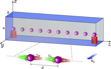
Figure 1: Chain of magnetic spheres with period $d$ in a microwave waveguide. The chain and waveguide are parallel to the $\hat{z}$-axis and magnetizations are oriented along $\hat{\mathbf{y}}$ by a magnetic field $H_{y}$. Every magnets interacts with all other magnets to the right ($\Sigma_{R}$) and left ($\Sigma_{L}$). Small coils attached to each magnet can excite and detect the local magnon accumulation (only two are shown).

The antenna array allows controlled excitation and detection of individual magnets as well as collective modes that is not possible by a global waveguide input and output. We predict that a chiral magnon-photon coupling in such an array leads to magnon edge states on one side of the chain. A large magnon amplitude can be generated by relatively weak excitation power, so our scheme is an alternative to parametric pumping [41; 42]. We envision that similar effects occur when a chiral interaction between magnets is mediated by other quasiparticles such as other magnons [43; 44], conduction electron spins [45] and phonons [46; 47]. This Letter is accompanied by a longer manuscript [48] that exposes the basic theory and focusses on the microwave scattering through a waveguide by more configurations including one, two, and many magnets.

Formalism.—We consider a waveguide along the $\hat{\mathbf{z}}$-direction with a rectangular cross section and model it by Maxwell’s equations with metallic boundary conditions. Even though the predicted effects obey classical physics, we use a quantum formalism for technical convenience as well as future research into quantum effects. The total Hamiltonian $\hat{H}_{\mathrm{em}}+\hat{H}_{\mathrm{m}}+\hat{H}_{\mathrm{int}}$ is of the Fano-Anderson type [49; 50; 51]. The photons form a set of harmonic oscillators:

$$\hat{H}_{\mathrm{em}}=\int\hbar\Omega_{k}\hat{p}_{k}^{\dagger}\hat{p}_{k}dk,$$ (1)

where $\hat{p}_{k}$ annihilates a photon with frequency $\Omega_{k}$ and momentum $k$ of the lowest transverse $\mathrm{TE}_{10}$ mode that is polarized along and uniformly distributed over the $\hat{\mathbf{y}}$-direction and with standing wavelength $2a$ in the $\hat{\mathbf{x}}$-direction (see Fig. 1 with $a>b$). The dispersion $\Omega_{k}^{2}/c^{2}=k^{2}+(m/a)^{2}+(n/b)^{2}\$and from now on $\{m,n\}=\{1,0\}$.

The waveguide is loaded with $N$ identical YIG spheres with gyromagnetic ratio $-\gamma$, saturation magnetization $M_{s}$, and volume $V_{s}$ at $\mathbf{r}_{j}=(\boldsymbol{\rho},(j-1)d)$ with $j\in\{1,2,\cdots,N\}$, where $\boldsymbol{\rho}=(x,y)$ and $d$ is the (equidistant) spacing between the spheres. The sub-mm spheres are much smaller than the photon wavelength of $\mathcal{O}\left(\mathrm{cm}\right)$, so they can be treated as point particles. The static magnetic field $H_{y}$ in the $\hat{\mathbf{y}}$-direction in Fig. 1 is sufficiently strong to saturate the magnetization. The waveguide photons couple to the anti-clockwise uniform magnetization precession around the magnetic field (Kittel mode). In second quantization

$$M_{j,z}-iM_{j,x}=\sqrt{{2\hbar\gamma M_{s}}/{V_{s}}}\hat{m}_{j},$$ (2)

where $M_{j,\delta}$ is the $\delta$-th component of the magnetization amplitude in the $j$-th magnet and $\hat{m}_{j}$ is a bosonic annihilation operator. The dynamics is governed by the linearized Landau-Lifshitz equation (damping to be included below), which after substituting Eq. (2) reduces to a harmonic oscillator for each magnet

$$\hat{H}_{\mathrm{m}}=\hbar\omega_{m}\sum_{j=1}^{N}\hat{m}_{j}^{\dagger}\hat{m}_{j},$$ (3)

where $\omega_{m}=\mu_{0}\gamma H_{y}$ is the Larmor precession frequency and $\mu_{0}$ is the vacuum permeability.

The photons and magnons are coupled by the Zeeman interaction

$$\hat{H}_{\mathrm{int}}=\sum_{j}\int\frac{dk}{\sqrt{2\pi}}\left[\hbar g_{j}(k)\hat{p}_{k}\hat{m}_{j}^{\dagger}+\mathrm{h.c.}\right].$$ (4)

The coupling constant $g_{j}(k)=\tilde{g}(k)e^{ik(j-1)d}$, where

$$\tilde{g}(k)=-\mu_{0}\sqrt{\frac{\gamma M_{s}V_{s}}{2\hbar}}\mathcal{H}_{k,-}\left(\boldsymbol{\rho}\right),$$ (5)

with $\mathcal{H}_{k,-}=\mathcal{H}_{k,z}-i\mathcal{H}_{k,x}$ being the microwave transverse magnetic field.

The magnons interact resonantly with photons with wave numbers near $k_{0}=\sqrt{\omega_{m}^{2}/c^{2}-\pi^{2}/a^{2}}$. The magnetic field of $\mathrm{TE}$-photons is polarization-momentum locked, i.e. $\mathcal{H}_{k,-}$ depends on the sign of $k$ [35; 37; 39; 40; 38; 36]. A magnet, e.g., kept at a position where $\mathcal{H}_{-k_{0},-}$ is zero but $\mathcal{H}_{k_{0},-}$ is finite, can radiate only into the $+\hat{\mathbf{z}}$-direction. For the $\mathrm{TE}_{10}$ mode this occurs for arbitrary $y$ and

$$\cot\left({\pi x}/{a}\right)=-\sqrt{k_{0}a}{\pi}.$$ (6)

The effective coupling between spheres can be modelled by integrating out the photon fields (for details see Ref. [48]) in terms of the equation of motion for the vector of magnetizations $\hat{\mathcal{M}}=\left(\hat{m}_{1},\dots,\hat{m}_{N}\right)^{T}$

$${d\hat{\mathcal{M}}}/{dt}=-i\tilde{H}_{\mathrm{eff}}\hat{\mathcal{M}}-\hat{\mathcal{T}}-\sqrt{\alpha_{G}\omega_{m}}\hat{\mathcal{N}}.$$ (7)

$\alpha_{G}\$is the Gilbert damping constant and $\hat{\mathcal{T}}=\hat{\mathcal{T}}_{w}+\hat{\mathcal{T}}_{l}$ is the external torque by the wave guide photons

$$\hat{\mathcal{T}}_{w}=i\int\frac{dk}{\sqrt{2\pi}}\tilde{g}(k)\hat{p}_{k,\mathrm{in}}e^{-i\Omega_{k}t}\left(e^{ikd},\cdots,e^{ikNd}\right)^{T},$$ (8)

and the local antennas $\hat{\mathcal{T}}_{l}=(\hat{P}_{1}(t),\cdots,\hat{P}_{N}(t))^{T}$. $\hat{\mathcal{N}}=\left(\hat{n}_{1},\cdots,\hat{n}_{N}\right)^{T}$ is the thermal noise in the magnetic system. We model $\hat{n}_{j}$ as white noise sources satisfying $\langle{\hat{n}_{j}}\rangle=\langle{\hat{n}_{j}\hat{n}_{i\neq j}}\rangle=0$, $\langle{\hat{n}_{j}^{\dagger}(t)\hat{n}_{j}(t^{\prime})}\rangle=n_{m}\delta(t-t^{\prime})$, $\langle{\hat{n}_{j}(t)\hat{n}_{j}^{\dagger}(t^{\prime})}\rangle=(n_{m}+1)\delta(t-t^{\prime})$, where $n_{m}=1/\left\{\exp\left[{\hbar\omega_{m}}/({k_{B}T})\right]-1\right\}$ is the thermal occupation of magnons at (constant) bath temperatures $T>\hbar\omega_{m}/k_{B}$ [52; 53].

In the non-Hermitian matrix $\tilde{H}_{\mathrm{eff}}=\tilde{\omega}+\Sigma$, $\tilde{\omega}_{jl}\equiv\tilde{\omega}_{m}\delta_{jl}=\omega_{m}\left(1-i\alpha_{G}\right)\delta_{jl}$, and the photon-mediated self-energy

$$\Sigma_{jl}=-i\begin{cases}(\Gamma_{L}+\Gamma_{R})/2,&j=l\\ \Gamma_{R}e^{ik_{0}(j-l)d},&j>l\\ \Gamma_{L}e^{ik_{0}(l-j)d},&j<l\end{cases},$$ (9)

where $\Gamma_{R}=\tilde{g}^{2}(k_{0})/v(k_{0}),\Gamma_{L}=\tilde{g}^{2}(-k_{0})/v(k_{0})$ and $v(k)=|k|c^{2}/\omega_{m}$ is the photon group velocity. The self-energy contributes to the dissipative and long-range coupling between any two magnets. The chiral coupling appears when $\Gamma_{L}\neq\Gamma_{R}$. The direct coupling between any two magnets does not depend on distance because we may safely disregard retardation and assume sufficiently high quality of the waveguide and magnets.

Hamiltonian.—The Hamiltonian $\tilde{H}_{\mathrm{eff}}$ is non-Hermitian, but can be diagonalized by introducing left and right eigenvectors [23]. The right eigenvectors of $\Sigma$, say $\{\psi_{\zeta}\}$ with corresponding eigenvalues $\{\gamma_{\zeta}\}$, satisfy $\left(\gamma_{\zeta}-\Sigma\right)\psi_{\zeta}=0$ for a delocalized mode with label $\zeta\in\{1,\dots,N\}$. Here $\mathrm{Re}\left[\gamma_{\zeta}\right]$ is the resonance frequency and $\mathrm{Im}\left[\gamma_{\zeta}\right]$ the reciprocal lifetime. $\{\phi_{\zeta}\}\neq\{\psi_{\zeta}\}$ are the eigenvectors of $\Sigma^{\dagger}$ with eigenvalues $\{\gamma_{\zeta}^{\ast}\}$. In the absence of degeneracies in $\{\gamma_{\zeta}\}$ the (normalized) modes are “bi-orthonormal”, i.e. $\phi_{\zeta}^{\dagger}\psi_{\zeta^{\prime}}=\delta_{\zeta\zeta^{\prime}}$ [26]. With $\Sigma^{\dagger}=\mathcal{P}\Sigma^{\ast}\mathcal{P}$ where $\mathcal{P}_{ij}=\delta_{i+j,N}$ inverts the order of magnets $1\leftrightarrow N$, $2\leftrightarrow N-1,$ $\cdots$, we arrive at $\phi_{\zeta}=\mathcal{P}\psi_{\zeta}^{\ast}$ [48].

$\tilde{H}_{\mathrm{eff}}$ consists of a Hermitian $\tilde{H}_{h}=(\tilde{H}_{\mathrm{eff}}+\tilde{H}_{\mathrm{eff}}^{\dagger})/2$ and non-Hermitian part $\tilde{H}_{nh}=(\tilde{H}_{\mathrm{eff}}-\tilde{H}_{\mathrm{eff}}^{\dagger})/2$. $\hat{\mathcal{M}}$ can be expanded into generalized Bloch states $\hat{\Psi}_{\kappa}=\sum_{j=1}^{N}e^{i{\kappa}z_{j}}\hat{m}_{j}/\sqrt{N}$ with $z_{j}=(j-1)d$ and complex “crystal momentum” $\kappa$. Two Bloch states $\hat{\Psi}_{k_{0}}$ and $\hat{\Psi}_{-k_{0}}$ diagonalize $\tilde{H}_{nh}$ (recall $k_{0}=\sqrt{\omega_{m}^{2}/c^{2}-\pi^{2}/a^{2}}$)

$$\begin{pmatrix}\nu+\frac{i}{2}\Gamma_{L}N&\frac{i}{2}\Gamma_{R}\frac{1-e^{2ik_{0}Nd}}{1-e^{2ik_{0}d}}\\ \frac{i}{2}\Gamma_{L}\frac{1-e^{-2ik_{0}Nd}}{1-e^{-2ik_{0}d}}&\nu+\frac{i}{2}\Gamma_{R}N\end{pmatrix}\begin{pmatrix}\hat{\Psi}_{k_{0}}\\ \hat{\Psi}_{-k_{0}}\end{pmatrix}=0.$$ (10)

The sum of the eigenvalues $\nu_{+}+\nu_{-}=-iN(\Gamma_{L}+\Gamma_{R})/2$ is the total radiative decay rate, which scales with the number of magnets. These two states are called “superradiant” or “bright”, while the remaining $(N-2)$ states are “subradiant” or “dark” with initially infinite radiative lifetime. The coherent coupling by $\tilde{H}_{h}$ mixes all states, but subradiant states with enhanced lifetimes persist, as we show below by a combined analytic and numerical treatment (see also Ref. [48]).

The ansatz of extended Bloch states $\hat{\Psi}_{\kappa}$ leads to the closed expression for the homogeneous Schrödinger equation [27]

$$d\hat{\Psi}_{\kappa}/dt=-i\omega_{\kappa}\hat{\Psi}_{\kappa}-\Gamma_{L}g_{\kappa}\hat{\Psi}_{k_{0}}+\Gamma_{R}h_{\kappa}\hat{\Psi}_{-k_{0}},$$ (11)

in which

$$\omega_{\kappa}\equiv-i\frac{\Gamma_{R}}{2}\frac{1+e^{i({\kappa}+k_{0})d}}{1-e^{i({\kappa}+k_{0})d}}+i\frac{\Gamma_{L}}{2}\frac{1+e^{i({\kappa}-k_{0})d}}{1-e^{i({\kappa}-k_{0})d}},$$ (12)

with $g_{\kappa}=1/[1-e^{i({\kappa}-k_{0})d}]$ and $h_{\kappa}={e^{i({\kappa}+k_{0})Nd}}/[1-e^{i({\kappa}+k_{0})d}].$ In an infinite chain (or a closed ring) $\hat{\Psi}_{\kappa}$ would be a solution. The boundary conditions of the finite system can be fulfilled by the superposition of two states with momenta $\kappa$ and $\kappa^{\prime}$ at the same frequency $\omega_{\kappa}=\omega_{\kappa^{\prime}}$. The additional terms appearing in Eq. (11) are cancelled by enforcing

$$g_{\kappa}h_{\kappa^{\prime}}=g_{\kappa^{\prime}}h_{\kappa},$$ (13)

leading to eigenstates $\hat{\alpha}_{\zeta}=\sum_{j}\phi_{\zeta,j}^{\ast}\hat{m}_{j}\propto(g_{\kappa}\hat{\Psi}_{\kappa^{\prime}}-g_{\kappa^{\prime}}\hat{\Psi}_{\kappa}).$ The wave functions and spectra then read

$$\psi_{\zeta,j}\propto g_{\kappa^{\prime}}e^{i\kappa z_{N-j}}-g_{\kappa}e^{i\kappa^{\prime}z_{N-j}};\;\gamma_{\zeta}=\omega_{\kappa}.$$ (14)

Only when the system is inversion symmetric ($\Gamma_{L}=\Gamma_{R}$), the solutions reduce to standing waves with $\operatorname{Re}\kappa^{\prime}=-\operatorname{Re}\kappa$.

$\omega_{\kappa}$ diverges at $\kappa=\pm k_{0}$. On the other hand, the radiative damping $\sim\mathrm{\operatorname{Im}}\omega_{\kappa}$ is minimized for say ${\kappa}={\kappa}_{\ast}.$ Neither $\kappa=\pm k_{0}$ nor $\kappa_{\ast}$ solve Eq. (13), but these states reflect the “superradiance” and “subradiance” well-known in quantum optics [26; 27; 28; 29; 30; 31]. The former corresponds to the edge states of $\tilde{H}_{\mathrm{eff}}\$with enhanced magnon amplitudes and damping, while the latter are weakly coupled delocalized standing waves, as demonstrated in the following.

The wave numbers ${\kappa}_{\ast}$ of the extremal points $\mathrm{\operatorname{Im}}\omega_{{\kappa}_{\ast}}$ obey

$${\kappa}_{\ast}d =\arcsin\frac{\Gamma_{R}-\Gamma_{L}}{\sqrt{\Gamma_{R}^{2}+\Gamma_{L}^{2}-2\Gamma_{R}\Gamma_{L}\cos(2k_{0}d)}}$$

$$-\arctan\frac{\Gamma_{R}-\Gamma_{L}}{(\Gamma_{R}+\Gamma_{L})\tan(k_{0}d)}.$$ (15)

$\arcsin x$ is a two-valued function in the first Brillouin zone $[-\pi/d,\pi/d]$ and we have two extremal points. The two solutions close to each extremum ${\kappa}_{\pm}={\kappa}_{\ast}\pm\delta$ label degenerate states that solve $g_{{\kappa}_{+}}h_{{\kappa}_{-}}=g_{{\kappa}_{-}}h_{{\kappa}_{+}}$. For small $\delta$,

$$\delta_{\zeta}=\frac{\zeta\pi}{Nd}\left[1-\frac{i}{N}\frac{\sin\left(k_{0}d\right)}{\cos\left({\kappa}_{\ast}d\right)-\cos\left(k_{0}d\right)}\right],$$ (16)

where $\zeta\in\mathbb{N}$. With Eq. (14), the wave function and dispersion of these subradiant states read

$$\psi_{\zeta,j} \approx-2i\frac{e^{i\kappa_{\ast}z_{N-j}}}{1-e^{i(\kappa_{\ast}-k_{0})d}}\sin(\delta_{\zeta}z_{N-j}),$$

$$\omega_{\zeta} =\omega_{{\kappa}_{\ast}}+\frac{\sin(k_{0}d)}{\cos({\kappa}_{\ast}d)-\cos(k_{0}d)}\frac{\Gamma_{R}(\delta_{\zeta}d)^{2}/2}{1-\cos[(k_{0}+{\kappa}_{\ast})d]},$$ (17)

where $\delta_{\zeta}\propto\zeta/(Nd)$. These solutions are nearly standing waves with long radiative lifetimes and are only weakly affected by chirality.

We have to numerically calculate the solutions for $\kappa$ close to $\pm k_{0}$, i.e. $\kappa=k_{0}+\eta$ and $\kappa^{\prime}=-k_{0}+\eta^{\prime}$ in which $\eta$ and $\eta^{\prime}$ are small complex numbers. $\operatorname{Im}\eta$ and $\operatorname{Im}\eta^{\prime}$ govern the decay of the states at the two edges. With chirality, only one of them is important, which causes a concentration at one edge of the chain.

As an example, we consider a rectangular waveguide with dimensions $a=1.6$ cm and $b=0.6$ cm, and $20$ YIG magnetic spheres with radius $r_{c}=0.6$ mm and $\alpha_{G}=5\times 10^{-5}$ [51]. $\omega_{m}/(2\pi)=\sqrt{3}c/\left(2a\right)=16.2$ GHz is tuned to correspond to the photon momentum $k_{0}=\sqrt{2}\pi/a$ of the lowest TE₁₀ mode. By varying the position and size of the magnets we may tune the magnon-photon interaction Eq. (9), here $\Gamma_{R,L}/(2\pi)\in(0,20)$ MHz, while $\alpha_{G}\omega_{m}/(2\pi)\sim 1$ MHz and chiralities $0<\Gamma_{L}/\Gamma_{R}<\infty$. $k_{0}d=\pi/5$, corresponds to an intermagnet spacing $d=a/(5\sqrt{2})\approx 0.2$ cm and $Nd\approx 4$ cm. The predicted features do not depend strongly on the chain lengths and are still prominent for a small number of spheres [48].

Magnon accumulation.—Figure 2 is a plot of the energy spectra and magnon accumulation (squared wave functions). Fig. 2(a) shows that the real and imaginary components of the eigen-energy $\gamma_{\zeta}$, scaled by $\Gamma_{a}=(\Gamma_{L}+\Gamma_{R})/2$, are approximately distributed on an ellipse in the complex plane that depends only weakly on the chirality. The solutions with long lifetimes are clustered around the frequencies $\omega_{\kappa_{\ast}}.$ It is negative in Fig. 2(a) but depends strongly on $k_{0}.$ Modes with $\mathrm{\operatorname{Im}}\gamma>\Gamma_{a}$ ($<\Gamma_{a}$) are super-radiant (subradiant) with radiative lifetime shorter (longer) than that of an isolated magnet. The decay rates of all eigenstates are sorted and plotted with integer labels $\zeta\in\{1,2,\cdots,20\}$ in Fig. 2(b). Here, the typical radiative lifetime of the most superradiant state $\left(\zeta=20\right)$ is $20\sim 70$ MHz for the three chiralities.

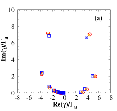
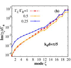
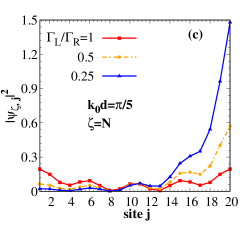
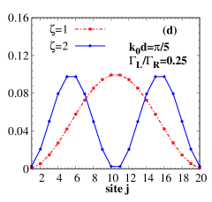
Figure 2: (Color online) Energy spectra and wave functions of the magnet chain of $20$ magnetic spheres. (a) Real and imaginary components of the eigen energies $\gamma=(\nu-\tilde{\omega}_{m})$ scaled by $\Gamma_{a}=(\Gamma_{L}+\Gamma_{R})/2$. Red circles, orange crosses and blue squares encode the chiralities $\Gamma_{L}/\Gamma_{R}=1$, 0.5 and 0.25, respectively. (b) All $20$ eigenstates sorted by increasing decay rates. (c) Magnon intensity distribution of the most short-lived state with $\zeta=20$ in (b). (d) Magnon intensity distribution for the longest living states with $\zeta=1,2$ in (b).

The magnon accumulation $|\psi_{\zeta,j}|^{2}$ of the most short-lived state ($\zeta=20$ in Fig. 2(b)) is plotted in Fig. 2(c). When $\Gamma_{R}=\Gamma_{L}$, the state is symmetrically localized close to both edges (red solid curve), but with increasing chirality, the distribution becomes asymmetrically skewed to one boundary. When $\Gamma_{R}<\Gamma_{L}$ ($\Gamma_{R}>\Gamma_{L}$), the boundary state is localized at the left (right) boundary of the chain. The enhanced dynamics associated to large magnon numbers causes superradiance. The most subradiant states, on the other hand, have magnon accumulations $\sim\left|\sin\left(\zeta\pi j/N\right)\right|^{2}$, with small amplitudes at the two boundaries, as shown in Fig. 2(d), and are only weakly affected by chirality. A weak higher harmonic reflects the bare photon wave length $\sim 2\pi/k_{0}$.

We can now expand the magnetization $\hat{\mathcal{M}}(t)=\sum_{\zeta=1}^{N}\hat{\alpha}_{\zeta}(t)\psi_{\zeta}$ into the above eigenstates with coefficients $\hat{\alpha}_{\zeta}(t)=\phi_{\zeta}^{\dagger}\hat{\mathcal{M}}(t)$. For the local input vector at common frequency $\omega_{\mathrm{in}}$, $\left\langle\hat{\mathcal{T}}_{l}(t)\right\rangle=ie^{-i\omega_{\mathrm{in}}t}\left(P_{1},P_{2},\cdots,P_{N}\right)$ and waveguide photon feed $\left\langle\hat{\mathcal{T}}_{w}\right\rangle=0$ (we discuss the case with $\left\langle\hat{\mathcal{T}}_{w}\right\rangle\neq 0$ and $\left\langle\hat{\mathcal{T}}_{l}\right\rangle=0$ in Ref. [48]), the coherent magnetization amplitude

$$\left\langle\hat{\mathcal{M}}(t)\right\rangle=-i\sum_{\zeta}\frac{(\mathcal{P}\psi_{\zeta})^{T}\left\langle\hat{\mathcal{T}}_{l}(t)\right\rangle}{\omega_{\mathrm{in}}-\tilde{\omega}_{m}-\gamma_{\zeta}}\psi_{\zeta}.$$ (18)

We are looking for a large magnon accumulation at one edge of the chain due to the chirality. Since $(\mathcal{P}\psi_{\zeta})^{T}=(\psi_{\zeta,N},\psi_{\zeta,N-1},\cdots,\psi_{1})$ oscillates between spheres with fixed phase, the vector product $(\mathcal{P}\psi_{\zeta})^{T}\left\langle\hat{\mathcal{T}}_{l}(t)\right\rangle$ can be large for a localized edge state ${\zeta_{\ast}}$ on the right when the input from the local antennas matches its phase and frequency. To match the phases of the edge states, we consider local power injection of the form $\left\langle\hat{\mathcal{T}}_{l}(t)\right\rangle=iP(1,e^{i\phi},\cdots,e^{i(N-1)\phi})\exp[-i(\omega_{m}+\mathrm{\operatorname{Re}}\gamma_{\zeta_{\ast}})t]$, in which the optimal phase depends on the number of magnets but $\phi$ $\rightarrow k_{0}d$ for sufficiently long chains.

Figure 3(a) shows that switching on the local antennas for $\Gamma_{L}/\Gamma_{R}=0.1$ and phase $\phi$ optimally chosen to be $\sim 0.44\pi$ leads to an enhanced accumulation on the right side. This choice of $\phi$ is out of phase with the subradiant states that are therefore hardly excited (see the blue curve in Fig. 3(a)). Fig. 3(b) is the accumulation on the right-most sphere as a function of chirality, which is enhanced more than 100-fold by tuning the chirality $\Gamma_{L}/\Gamma_{R}\rightarrow 0.$ In this limit the frequencies become degenerate, but individual modes can still be accessed by the phased array.

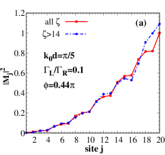
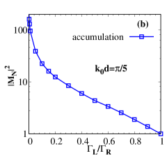
Figure 3: (Color online) Magnon accumulation excited by a phased antenna array. (a), The accumulation (squared magnetization amplitude) distribution over the magnets (red cureve) is normalized by the largest value at the edge. The blue curve excludes the contribtuion of subradiant states. (b), The magnon accumulation at the right edge as a function of chirality, normalized by the one for $\Gamma_{L}/\Gamma_{R}=1$.

Conclusions.—In conclusion, the interaction between magnons and photons can be chiral and tunable by strategically positioning small magnets in a waveguide. We predict a strong imbalance of magnon populations in a chain of magnets in which the dissipative and long-range nature of the coupling can strongly enhance the magnon intensity at the edges. The coherent amplitudes of magnons at one edge of the sample can be much higher than those excited by conventional ferromagnetic resonance. This allows studying non-linear effects at low input power. On the other hand, the magnon number of the magnets in the center of the chain are only weakly affected.

Our formalism can be extended into the quantum regime of magnons, in which we can profit from the insights of the field of quantum optics, which studies collective coupling with atomic emitters [26; 27; 28; 29; 30]. The strong coupling between magnons and photons in a microwave waveguide [51] opens the new perspective of magnonic quantum emitters [54], which might help circumventing the harsh experimental environment such as extremely low temperature and fine control required for cold atom system. We also find analogies with chiral optics, in which the coupling between light and emitters depends on the propagation of light and polarization of the local emitters [36]. The chiral coupling between emitters is promising in achieving quantum state transfer between qubits via the magnonic chiral quantum channel introduced here.

- [1] A. Auerbach, Interacting Electrons and Quantum Magnetism (Springer-Verlag, New York, 1994).
- [2] M. A. Ruderman and C. Kittel, Phys. Rev. 96, 99 (1954); T. Kasuya, Prog. Theor. Phys. 16, 45 (1956); K. Yosida, Phys. Rev. 106, 893 (1957).
- [3] H. Suhl, Phys. Rev. 109, 606 (1958).
- [4] T. Nakamura, Progr. Theoret. Phys. (Kyoto) 20, 542 (1958).
- [5] L. Mandel and E. Wolf, Optical Coherence and Quantum Optics (Cambridge University Press, Cambridge, England, 1995).
- [6] Ö. O. Soykal, and M. E. Flatté, Phy. Rev. Lett. 104, 077202 (2010).
- [7] H. Huebl, C. W. Zollitsch, J. Lotze, F. Hocke, M. Greifenstein, A. Marx, R. Gross, and S. T. B. Goennenwein, Phy. Rev. Lett. 111, 127003 (2013).
- [8] Y. Tabuchi, S. Ishino, T. Ishikawa, R. Yamazaki, K. Usami, and Y. Nakamura, Phy. Rev. Lett. 113, 083603 (2014).
- [9] X. Zhang, C.-L. Zou, L. Jiang, and H. X. Tang, Phy. Rev. Lett. 113, 156401 (2014).
- [10] X. Zhang, C.-L. Zou, N. Zhu, F. Marquardt, L. Jiang, and H. X. Tang, Nat. Comm. 6, 8914 (2015).
- [11] N. J. Lambert, J. A. Haigh, S. Langenfeld, A. C. Doherty, and A. J. Ferguson, Phys. Rev. A 93, 021803(R) (2016).
- [12] B. Z. Rameshti and G. E. W. Bauer, Phys. Rev. B 97, 014419 (2018).
- [13] N. Hatano and D. R. Nelson, Phys. Rev. Lett. 77, 570 (1996).
- [14] C. M. Bender, D. C. Brody, and H. F. Jones, Phys. Rev. Lett. 89, 270401 (2002).
- [15] C. M. Bender, D. C. Brody, H. F. Jones, and B. K. Meister, Phys. Rev. Lett. 98, 040403 (2007).
- [16] D. Zhang, X.-Q. Luo, Y.-P. Wang, T.-F. Li, and J. Q. You, Nat. Commun. 8, 1368 (2017).
- [17] R. El-Ganainy, K. G. Makris, M. Khajavikhan, Z. H. Musslimani, S. Rotter, and D. N. Christodoulides, Nat. Phys. 14, 11 (2018).
- [18] S. Y. Yao and Z. Wang, Phys. Rev. Lett. 121, 086803 (2018).
- [19] Z. Gong, Y. Ashida, K. Kawabata, K. Takasan, S. Higashikawa, and M. Ueda, Phys. Rev. X. 8, 031079 (2018).
- [20] X. S. Yang, Y. Cao, and Y. Zhai, arXiv:1904.02492.
- [21] S. Y. Yao, F. Song and Z. Wang, Phys. Rev. Lett. 121, 136802 (2018).
- [22] H. Jiang, L. J. Lang, C. Yang, S. L. Zhu, and S. Chen, Phys. Rev. B 100, 054301 (2019).
- [23] N. Moiseyev, Non-Hermitian Quantum Mechanics, (Cambridge University Press, Cambridge, 2011).
- [24] M. Harder, Y. Yang, B. M. Yao, C. H. Yu, J. W. Rao, Y. S. Gui, R. L. Stamps, and C.-M. Hu, Phys. Rev. Lett. 121, 137203 (2018).
- [25] B. M. Yao, T. Yu, X. Zhang, W. Lu, Y. S. Gui, C.-M. Hu, and Y. M. Blanter, arXiv:1906.12142.
- [26] A. Asenjo-García, M. Moreno-Cardoner, A. Albrecht, H. J. Kimble, and D. E. Chang, Phys. Rev. X 7, 031024 (2017).
- [27] Y.-X. Zhang and K. Mølmer, Phys. Rev. Lett. 122, 203605 (2019).
- [28] M. M. Cardoner, D. Plankensteiner, L. Ostermann, D. E. Chang, and H. Ritsch, Phys. Rev. A 100, 023806 (2019).
- [29] P.-O. Guimond, A. Grankin, D. V. Vasilyev, B. Vermersch, and P. Zoller, Phys. Rev. Lett. 122, 093601 (2019).
- [30] G. Buonaiuto, R. Jones, B. Olmos, and I. Lesanovsky, arXiv:1902.08525.
- [31] J. Li, S. Y. Zhu, and G. S. Agarwal, Phys. Rev. Lett. 121, 203601 (2018).
- [32] L. M. Sieberer, S. D. Huber, E. Altman, and S. Diehl, Phys. Rev. Lett. 110, 195301 (2013).
- [33] S. Diehl, A. Micheli, A. Kantian, B. Kraus, H. P. Büchler, and P. Zoller, Nat. Phys. 4, 878 (2008).
- [34] N. Bernier, E. Torre, and E. Demler, Phys. Rev. Lett. 113, 065303 (2014).
- [35] J. D. Jackson, Classical Electrodynamics, (Wiley, New York, 1998).
- [36] P. Lodahl, S. Mahmoodian, S. Stobbe, A. Rauschenbeutel, P. Schneeweiss, J. Volz, H. Pichler, and P. Zoller, Nature (London) 541, 473 (2017).
- [37] F. Le Kien, S. D. Gupta, K. P. Nayak, and K. Hakuta, Phys. Rev. A 72, 063815 (2005).
- [38] B. le Feber, N. Rotenberg, and L. Kuipers, Nat. Commun. 6, 6695 (2015).
- [39] M. Scheucher, A. Hilico, E. Will, J. Volz, and A. Rauschenbeutel, Science 354, 1577 (2016).
- [40] B. Vermersch, P.-O. Guimond, H. Pichler, and P. Zoller, Phys. Rev. Lett. 118, 133601 (2017).
- [41] A. G. Gurevich and G. A. Melkov, Magnetization Oscillations and Waves (CRC, New York, 1996).
- [42] V. S. L’vov, Wave Turbulence under Parametric Excitations: Applications to Magnetics (Springer, Berlin, 1994).
- [43] T. Yu, C. P. Liu, H. M. Yu, Y. M. Blanter, and G. E. W. Bauer, Phys. Rev. B 99, 134424 (2019).
- [44] J. L. Chen, T. Yu, C. P. Liu, T. Liu, M. Madami, K. Shen, J. Y. Zhang, S. Tu, M. S. Alam, K. Xia, M. Z. Wu, G. Gubbiotti, Y. M. Blanter, G. E. W. Bauer, and H. M. Yu, arXiv:1903.00638.
- [45] Y. Tserkovnyak, A. Brataas, G. E. W. Bauer, and B. I. Halperin, Rev. Mod. Phys., 77, 1375 (2005).
- [46] A. Kamra, H. Keshtgar, P. Yan, and G. E. W. Bauer, Phys. Rev. B 91, 104409 (2015).
- [47] S. Streib, H. Keshtgar, and G. E. W. Bauer, Phys. Rev. Lett. 121, 027202 (2018).
- [48] T. Yu, X. Zhang, S. Sharma, Y. M. Blanter, and G. E. W. Bauer, submitted to Physical Review B.
- [49] U. Fano, Phys. Rev. 124, 1866 (1961).
- [50] G. D. Mahan, Many Particle Physics (Plenum, New York, 1990).
- [51] B. M. Yao, T. Yu, Y. S. Gui, J. W. Rao, Y. T. Zhao, W. Lu, and C.-M. Hu, arXiv: 1902.06795.
- [52] C. W. Gardiner and M. J. Collett, Phys. Rev. A 31, 3761 (1985).
- [53] A. A. Clerk, M. H. Devoret, S. M. Girvin, F. Marquardt, and R. J. Schoelkopf, Rev. Mod. Phys. 82, 1155 (2010).
- [54] V. E. Demidov, S. Urazhdin, G. de Loubens, O. Klein, V. Cros, A. Anane, and S. O. Demokritov, Phys. Rep. 673, 1 (2017).