Joint Estimation of OD Demands and Cost Functions in Transportation Networks from Data 1

Abstract

Existing work has tackled the problem of estimating Origin-Destination (OD) demands and recovering travel latency functions in transportation networks under the Wardropian assumption. The ultimate objective is to derive an accurate predictive model of the network to enable optimization and control. However, these two problems are typically treated separately and estimation is based on parametric models. In this paper, we propose a method to jointly recover nonparametric travel latency cost functions and estimate OD demands using traffic flow data. We formulate the problem as a bilevel optimization problem and develop an iterative first-order optimization algorithm to solve it. A numerical example using the Braess Network is presented to demonstrate the effectiveness of our method.

I INTRODUCTION

The purpose of solving the Traffic Assignment Problem (TAP) in transportation planning processes is to evaluate performance metrics of the system, assess deficiencies and evaluate potential improvements and capacity expansions to the transportation network.

The TAP assumes that users selfishly choose the best route in the network resulting in an equilibrium known as Wardrop equilibrium. Modeling drivers’ routing behavior under the Wardrop equilibrium assumption is one of the most widely-used frameworks for the purpose of analyzing transportation networks, with applications in traffic diagnosis, control, and optimization [1, 2]. This modeling framework uses three main inputs: $(1)$ a strongly connected directed graph; $(2)$ an Origin Destination (OD) traffic demand vector; and $(3)$ a link latency cost or travel time cost function that typically depends on link flows. Small perturbations to these OD demand estimates and travel time functions may have a large impact on the equilibrium solution [3].

In practice, however, OD demands and cost functions are not readily available. The OD demand estimation problem for the static TAP has been solved differently depending on whether a network is congested or not. For uncongested networks, entropy maximization [4], generalized least squares [5] and maximum likelihood estimation [6] have been used. Whereas for congested networks, estimating OD demands has been done by solving a bilevel optimization problem given the circular dependence between the OD estimation and the traffic flow assignment [7].

The problem of estimating travel time functions has received less attention in the transportation community. In the context of transportation systems, as traffic volume grows we expect the speed on the link to decrease, first slowly but as queues start to accumulate, the effects become more significant. Therefore, these functions are usually modeled as positive, nonlinear and strictly increasing functions. A typical travel time function is as a polynomial function. In particular, urban planners and researchers often use the Bureau of Public Roads (BPR) function [8]:

$$t(x_{a})=t_{a}^{0}(1+0.15(x_{a}/m_{a})^{4}),$$ (1)

where $t_{a}^{0}$ is the free-flow travel time, $x_{a}$ the flow, and $m_{a}$ the capacity of link $a$.

With the increasing availability of various sensors, large traffic datasets have been collected, raising the possibility of estimating OD demands and travel time functions from data by solving appropriate inverse optimization problems. More specifically, given an OD demand and equilibrium flows, recovering the travel time function can be performed for both single-class vehicle networks [3, 9] and multi-class vehicle networks [10].

Most of the existing work typically deals with these two inverse problems separately; a limitation we seek to address in this paper. Closer to the goal of our work, [11] considered the simultaneous estimation of travel cost and OD demand in a Stochastic User Equilibrium setting. Yet, this work does not attempt to estimate (nonparametrically) the full structure of the travel cost functions as we do. Rather, it seeks to estimate a sensitivity constant that adjusts how a given travel cost function affects route choice probabilities.

In this paper, we aim to jointly investigate the two related inverse problems – recovering cost functions (IP-1) in a non-parametric setting and adjusting OD demand matrices (IP-2). Our work contributes to improving the consistency and robustness of the data-driven traffic model. The ultimate utility of obtaining such a model is to use it to make predictions under various topology and demand scenarios, drive control and optimization tasks, or simply assess the amount of inefficiency of the system (e.g., as in  [10]). In this work we consider only the (data-driven) model estimation problem.

We solve the joint problem by converting the bilevel optimization model into a single-level one. We do this by transforming the lower-level problem (IP-1) into constraints for the upper-level one (IP-2). As a result, we obtain a formulation with a quadratic objective and non-convex constraints. Using weak duality and an iterative approach, we are able to relax the non-convex constraints, which allows the problem to be solved using a first-order feasible direction algorithm. To validate its effectiveness and performance, we conduct a numerical experiment using the Braess’ network [12]. In this example, we show that the algorithm approaches the ground truth values of both travel time functions and OD demands.

The rest of the paper is organized as follows. In Sec. II we introduce the modeling framework and mathematical definitions used throughout the paper. In Sec. III we present the structure of the joint problem, its transformation to its Frank-Wolfe form, and a method for calculating the gradient of the cost function. In Sec. IV we present some numerical results applied to the Braess network. Conclusions are in Sec. V.

Notation: All vectors are column vectors and denoted by bold lowercase letters. Bold uppercase letters denote matrices. To economize space, we write ${\mathbf{x}}=(x_{1},\ldots,x_{\text{dim}({\mathbf{x}})})$ to denote the column vector $\mathbf{x}$, where $\text{dim}({\mathbf{x}})$ is its dimensionality. We use “prime” to denote the transpose of a matrix or vector. We denote by ${\mathbf{0}}$ and ${\mathbf{I}}$ the vector of all zeroes and the identity matrix, respectively. Unless otherwise specified, $\|\cdot\|$ denotes the $\ell_{2}$ norm. $|\mathcal{D}|$ denotes the cardinality of a set $\mathcal{D}$, and $\left[\kern-1.49994pt\left[\mathcal{D}\right]\kern-1.49994pt\right]$ the set $\{1,\ldots,|\mathcal{D}|\}$.

II MODEL AND PRELIMINARIES

II-A Transportation network model and definitions

Consider a strongly-connected directed graph denoted by $G\left(\mathcal{V},\mathcal{A}\right)$, where $\mathcal{V}$ is the set of nodes and $\mathcal{A}$ is the set of links. Let $\mathbf{N}\in{\left\{{0,1,-1}\right\}^{\left|\mathcal{V}\right|\times\left|\mathcal{A}\right|}}$ be the node-link incidence matrix, and let $\textbf{e}_{a}\in\mathbb{R}^{|\mathcal{A}|}$ be a vector with an entry equal to $1$ corresponding to link $a$ and all the other entries set to $0$. Let $\mathbf{w}=(w_{s},w_{t})$ denote an Origin-Destination (OD) pair and $\mathcal{W}=\left\{{{\mathbf{w}_{i}}:{\mathbf{w}_{i}}=\left({{w_{si}},{w_{ti}}}\right),\,i\in\left[\kern-1.49994pt\left[\mathcal{W}\right]\kern-1.49994pt\right]}\right\}$ be the set of all OD pairs. Furthermore, let ${d^{\mathbf{w}}}\geq 0$ be the flow demand that travels from origin $w_{s}$ to destination $w_{t}$. In the same manner, let us denote by $\mathbf{d^{w}}\in\mathbb{R}^{|\mathcal{V}|}$ the vector of all zeros except for the coordinates of nodes $w_{s}$ and $w_{t}$ which take values $-d^{\mathbf{w}}$ and $d^{\mathbf{w}}$, respectively. We will also use vector ${\mathbf{g}}=(d^{{\mathbf{w}}};{\mathbf{w}}\in\mathcal{W})$ to denote the flow demands for all OD pairs. Let $x_{a}$ be the total link flow of link $a\in\mathcal{A}$ and $\mathbf{x}$ the vector of these flows. Let $\mathcal{F}$ be the set of feasible flow vectors defined by

$$\mathcal{F}=\Big{\{}\mathbf{x}\in\mathbb{R}_{+}^{|\mathcal{A}|}:\mathbf{x}=\sum\limits_{\mathbf{w}\in\mathcal{W}}{{\mathbf{x}^{\mathbf{w}}}},\,\mathbf{N}{\mathbf{x}^{\mathbf{w}}}={\mathbf{d}^{\mathbf{w}}},\,\forall\mathbf{w}\in\mathcal{W}\Big{\}},$$

where $\mathbf{x}^{\mathbf{w}}$ is the flow vector attributed to OD pair $\mathbf{w}$.

For each OD pair ${\mathbf{w}}$ let us also define a set of possible routes $\mathcal{R}^{{\mathbf{w}}}$; each route $r\in\mathcal{R}^{{\mathbf{w}}}$ is a sequence of links starting from the origin $w_{s}$ and ending at the destination $w_{t}$. We will write $a\in r$ if a route $r$ contains link $a$. For each OD pair ${\mathbf{w}}_{i}\in\mathcal{W}$ we define the indicator functions

$$\delta_{r}^{ai}=\begin{cases}1,&\text{if }r\in\mathcal{R}^{{\mathbf{w}}_{i}}\text{ uses link }a\\ 0,&\text{otherwise.}\end{cases}$$ (2)

Finally, we denote with $t_{a}(\mathbf{x}):\mathbb{R}_{+}^{\left|\mathcal{A}\right|}\mapsto\mathbb{R}_{+}$ the latency cost (i.e., travel time) function for link $a$ and write ${\mathbf{t}}(\cdot)$ for the vector of these link functions. Using the same structure used in [13] we can characterize $t_{a}(x_{a})$ as:

$$t_{a}(x_{a})=t_{a}^{0}f(x_{a}/m_{a}),$$

where $m_{a}$ is the flow capacity of link $a$, $f(\cdot)$ is a strictly increasing, positive, and continuously differentiable function, and $t_{a}^{0}$ is the free-flow travel time on link $a$. We set $f(0)=1$, which ensures that if there is no constraint on flow capacity, the travel time $t_{a}$ is equal to the free-flow travel time.

II-B Wardrop equilibrium

The notion of a Wardrop equilibrium, sometimes referred to as a non-atomic game, is interpreted as requiring that all users optimize their travel times. In general, a feasible flow $\mathbf{x^{*}}$ is a Wardrop equilibrium if for every OD pair $\mathbf{w}_{i}$, and any route $r\in\mathcal{R}^{{\mathbf{w}}_{i}}$ with positive flow, the latency cost (i.e., travel time) is no greater than the travel time on any other route. It is worth mentioning that given $G(\mathcal{V},\mathcal{A})$ and $f(\cdot)$ there exists a unique equilibrium. Such a result is the solution to the Traffic Assignment Problem (TAP) which precisely returns the flows that minimize the potential function:

$$\Phi(\mathbf{x})=\sum\limits_{a\in\mathcal{A}}\int\limits_{0}^{x_{a}}t_{a}(s)ds,$$

where the integral is adding the costs of the flow segments of link $a$. The function $f(\cdot)$ is continuous and $\mathcal{F}$ is a compact set, thus, Weierstrass Theorem implies there exists a solution. Moreover, since cost functions are non-decreasing (by assumption), then $\Phi(\cdot)$ is convex and therefore a unique solution exists [13].

II-C Models

II-C1 User-centric

As stated in the previous section, the TAP (also known as the user-centric forward optimization problem) can be formulated as

$$\min_{\mathbf{x}\in\mathcal{F}}\ \ \sum\limits_{a\in\mathcal{A}}{\int\limits_{0}^{x_{a}}{t_{a}(s)ds}}.$$ (3)

An alternative way of solving this problem is via a Variational Inequality (VI) formulation as first proposed in [14, 15]; finding a solution ${\mathbf{x}}^{*}$ to

$$\mathbf{t}(\mathbf{x}^{*})^{\prime}(\mathbf{x}-\mathbf{x^{*}})\geq 0,\ \ \forall\mathbf{x}\in\mathcal{F}.$$ (4)

In order for the solution of (4) to be equivalent to the solution of (3) we have to assume $(i)$ strong monotonicity of $\mathbf{t}(\cdot)$ over $\mathcal{F}$, $(ii)$ $\mathbf{t}(\cdot)$ to be continuously differentiable over $\mathbb{R}_{+}^{|\mathcal{A}|}$, and $(iii)$ $\mathcal{F}$ to contain an interior point (Slater’s condition). One of the most successful algorithms to find such an equilibrium is the Method of Successive Averages (MSA) proposed in [16] which uses a Frank-Wolfe type algorithm.

II-C2 User-Centric Inverse Model (I-VI)

Given that one of the parameters of the TAP is the latency cost functions, we aim to estimate them (in particular function $f(\cdot)$) using data. To that end, we consider an Inverse Variational Inequality problem (I-VI). We assume that the data measurements are solutions of the TAP for specific cost functions and OD demands. Therefore, it is natural to think about these flows as snapshots of the network at different instants. Let $k\in\left[\kern-1.49994pt\left[\mathcal{K}\right]\kern-1.49994pt\right]$ index different snapshots of a network with corresponding flows $\mathbf{x}^{(k)}=(x_{a}^{(k)};\ a\in\mathcal{A}^{(k)})$, where the set $\mathcal{A}^{(k)}\subset\mathcal{A}$ denotes the links on which we have flow measurements for instance $k$. (We will use $\mathcal{F}^{(k)}$, ${\mathbf{N}}_{k}$, and $\mathcal{W}^{(k)}$ to denote the set of feasible flows, node-link incidence matrix, and OD pairs for the network instance $k$.) The inverse formulation of the Wardrop equilibrium seeks to find a cost function ${\mathbf{t}}(\cdot)$ (or, equivalently, $f(\cdot)$) such that each flow observation is as close to an equilibrium as possible. Because this formulation relies on measured data, we expect measurement noise. Hence, the notion of an approximate solution to this problem is natural. For a given $\epsilon>0$, we define an $\epsilon$-approximate solution $\hat{{\mathbf{x}}}$ to the VI as satisfying:

$$\mathbf{t}(\hat{\mathbf{x}})^{\prime}(\mathbf{x}-\hat{\mathbf{x}})\geq-\epsilon,\ \ \forall\mathbf{x}\in\mathcal{F}.$$ (5)

The inverse VI problem amounts to finding a function ${f(\cdot)}$ such that $\mathbf{x}^{(k)}$ is an $\epsilon_{k}$-approximate solution to VI$(\mathbf{t},\mathcal{F}^{{(k)}})$ for each $k$. Denoting $\boldsymbol{\epsilon}\stackrel{{\scriptstyle\triangle}}{{=}}(\epsilon_{k};\,k\in[\kern-1.49994pt[\mathcal{K}]\kern-1.49994pt])$, we can formulate the inverse VI problem as in [3, 10]. Then we define the (I-VI) problem as minimizing the $\ell_{2}$ norm of $\boldsymbol{\epsilon}$:

$$\min_{{\mathbf{t}}(\cdot),\boldsymbol{\epsilon}} \ \ \|\boldsymbol{\epsilon}\|$$ (6)

s.t. $$\ \ \mathbf{t}(\mathbf{x}^{(k)})^{\prime}(\mathbf{x}-\mathbf{x}^{(k)})\geq-\epsilon_{k},\hskip 14.22636pt\forall\mathbf{x}\in\mathcal{F}^{(k)},k\in\left[\kern-1.49994pt\left[\mathcal{K}\right]\kern-1.49994pt\right],$$

$$\ \ \epsilon_{k}>0,\qquad\forall k\in\left[\kern-1.49994pt\left[\mathcal{K}\right]\kern-1.49994pt\right].$$

Notice that in this formulation, the set of constraints restricts the travel time function to be within $\epsilon_{k}$ units of the Wardrop equilibrium flows for each sample. In this sense, if we solve the problem using $k$ of these constraints for multiple observed networks, we will find a more “stable” travel time function.

In order to solve this problem we express the function $f(\cdot)$ in a Reproducing Kernel Hilbert Space (RKHS) $\mathcal{H}$ as in [3]. This leads to the following formulation of the $\epsilon$-approximate Inverse Variational Inequality Problem ($\epsilon$I-VI):

$$\min_{f,{\mathbf{y}},\boldsymbol{\epsilon}} \ \ \|\boldsymbol{\epsilon}\|+\gamma\|f\|^{2}_{\mathcal{H}}$$ (7)

s.t. $$\ \ \mathbf{e}_{a}^{\prime}\mathbf{N}_{k}^{\prime}\mathbf{y}^{\mathbf{w}}\leq t^{0}_{a}f\left(\frac{x_{a}}{m_{a}}\right),\forall\mathbf{w}\in\mathcal{W}^{(k)},a\in\mathcal{A}^{(k)},k,$$

$$\ \ \sum_{a\in\mathcal{A}^{(k)}}t^{0}_{a}x_{a}f\left(\frac{x_{a}}{m_{a}}\right)-\sum_{{\mathbf{w}}\in\mathcal{W}^{(k)}}(\mathbf{d^{w}})^{\prime}\mathbf{y^{w}}\leq\epsilon_{k},\forall k,$$

$$\ \ f\left(\frac{x_{a}}{m_{a}}\right)\leq f\left(\frac{x_{\hat{a}}}{m_{\hat{a}}}\right),\forall a,\hat{a}\in\cup_{k}\mathcal{A}^{(k)}\,\text{s.t.}\,\frac{x_{a}}{m_{a}}\leq\frac{x_{\hat{a}}}{m_{\hat{a}}},$$

$$\ \ \boldsymbol{\epsilon}\geq 0,\;f\in\mathcal{H},f(0)=1,$$

where the first constraint corresponds to dual feasibility, the second constraint maintains the primal-dual gap within $\epsilon$, and the third constraint imposes the assumption that $f(\cdot)$ is monotone. We note that $\mathbf{y^{w}}$ contains dual variables associated with the VI problem, $\|\cdot\|_{\mathcal{H}}$ is the norm of the RKHS, and $\gamma$ is a regularization parameter. A larger $\gamma$ will recover a more general $f(\cdot)$ whereas a smaller one will recover an $f(\cdot)$ which fits the dataset better.

As we can see, the problem we have defined is still hard to solve since it involves optimization over functions $f(\cdot)$. However, we specify $\mathcal{H}$ (and thus the class of $f(\cdot)$) by choosing a polynomial kernel [3], i.e., using kernel functions $\phi(x,y)=(c+xy)^{n}$. We believe this is a good choice since it matches our intuition on how congestion affects the latency cost of links (cf. (1)). The polynomial kernel function can be rewritten as

$$\phi(x,y)=(c+xy)^{n}=\sum\limits_{i=0}^{n}{n\choose i}c^{n-1}x^{i}y^{i}.$$

Then, using the representer theorem for kernel functions, we can modify the cost function of the ($\boldsymbol{\epsilon}$I-VI) problem to a quadratic function parameterized by $\boldsymbol{\beta}=\{\beta_{j}:j=1,\ldots,n\}$ resulting in a tractable Quadratic Programming (QP) problem (see [3, 10] for details). As an output to this reformulated ($\boldsymbol{\epsilon}$I-VI) problem we obtain $\boldsymbol{\beta}^{*}$, and therefore our estimator for $f(\cdot)$ is equal to

$$\hat{f}(x)=\sum\limits_{i=0}^{n}\beta_{i}^{*}x^{i}=1+\sum\limits_{i=1}^{n}\beta_{i}^{*}x^{i},$$

where we set $\beta_{0}=1$ to have $f(0)=1$.

To facilitate the analysis of the joint problem presented in the next section, let us write the QP problem corresponding to ($\boldsymbol{\epsilon}$I-VI) using compact notation:

$$\min_{\boldsymbol{\beta},{\mathbf{y}},\boldsymbol{\epsilon}} \ \ \boldsymbol{\epsilon}^{\prime}\mathbf{I}\boldsymbol{\epsilon}+\boldsymbol{\beta}^{\prime}\mathbf{H}\boldsymbol{\beta}$$ (8)

s.t. $$\ \ \mathbf{A}({\mathbf{g}}){\mathbf{y}}+\mathbf{B}({\mathbf{x}})\boldsymbol{\beta}+\mathbf{C}\boldsymbol{\epsilon}+{\mathbf{h}}\leq\boldsymbol{0},$$

where matrices $\mathbf{A}({\mathbf{g}})$ and $\mathbf{B}({\mathbf{x}})$ depend on the OD demand vector ${\mathbf{g}}$ and the provided data flow measurements $\mathbf{x}$, respectively, and $\mathbf{H}$ is a positive definite matrix. We call this problem (IP-1).

III THE JOINT PROBLEM

III-A Bilevel formulation

Unlike previous work, we will jointly recover both the travel time function $f(\cdot)$, specifically the coefficients $\boldsymbol{\beta}=(\beta_{o},\ldots,\beta_{n})$, and the OD demand vector ${\mathbf{g}}$. To simplify notation, we let $\mathbf{x}(\boldsymbol{\beta},{\mathbf{g}})=(x_{a}(\boldsymbol{\beta},{\mathbf{g}});\ \forall a\in\mathcal{A})$ be the optimal solution to the VI$(\mathbf{t},\mathcal{F})$ (i.e., the TAP), for any given feasible $\boldsymbol{\beta}$ and ${\mathbf{g}}$. Recall that we observe an equilibrium flow vector from data which we define as $\mathbf{x^{*}}=(x_{a}^{*};\ \forall a\in\mathcal{A})$. Equipped with these definitions we can define the bilevel optimization problem as follows

$$\min_{\boldsymbol{\beta},{\mathbf{g}}} \ \ F(\boldsymbol{\beta},{\mathbf{g}})\stackrel{{\scriptstyle\triangle}}{{=}}\sum_{a\in\mathcal{A}}(x_{a}(\boldsymbol{\boldsymbol{\beta}},{\mathbf{g}})-x_{a}^{*})^{2}$$ (9)

s.t. $$(\boldsymbol{\beta},{\mathbf{y}},\boldsymbol{\epsilon})=\arg\min_{\boldsymbol{\beta},{\mathbf{y}},\boldsymbol{\epsilon}}\big{\{}\boldsymbol{\epsilon}^{\prime}\mathbf{I}\boldsymbol{\epsilon}+\boldsymbol{\beta}^{\prime}\mathbf{H}\boldsymbol{\beta},$$

$$\text{s.t. }\mathbf{A}({\mathbf{g}}){\mathbf{y}}+\mathbf{B}({\mathbf{x}}(\boldsymbol{\beta},{\mathbf{g}}))\boldsymbol{\beta}+\mathbf{C}\boldsymbol{\epsilon}+{\mathbf{h}}\leq\boldsymbol{0}\big{\}},$$

$$\boldsymbol{\boldsymbol{\beta}}\geq\mathbb{0},\ {\mathbf{g}}\geq\mathbb{0}.$$

Notice that $F(\boldsymbol{\beta},{\mathbf{g}})$ is bounded below by $0$.

To solve this problem we replace the convex lower-level problem (IP-1) by its KKT optimality conditions and write the bilevel problem as a single-level problem. Finally, we relax the resulting formulation to make it solvable by using a feasible direction method (Frank-Wolfe).

III-B IP-1 Optimality conditions

To reduce the lower level problem in (9) into its equivalent optimality conditions, we first write the Lagrangian function:

$$\mathcal{L}(\boldsymbol{\beta},{\mathbf{y}},\boldsymbol{\epsilon};\boldsymbol{\nu})=\boldsymbol{\epsilon}^{\prime}\mathbf{I}\boldsymbol{\epsilon}+\boldsymbol{\beta}^{\prime}\mathbf{H}\boldsymbol{\beta}+\boldsymbol{\nu}^{\prime}(\mathbf{A}{\mathbf{y}}+\mathbf{B}\boldsymbol{\beta}+\mathbf{C}\boldsymbol{\epsilon}+{\mathbf{h}}),$$

where $\boldsymbol{\nu}$ are the dual variables and (for ease of notation) we dropped the dependence of ${\mathbf{A}}$ and ${\mathbf{B}}$ on ${\mathbf{g}}$ and ${\mathbf{x}}(\boldsymbol{\beta},{\mathbf{g}})$, respectively.

This leads to the first order optimality conditions:

$$\partial\mathcal{L}/\partial\boldsymbol{\epsilon} = 2\mathbf{I}\boldsymbol{\epsilon}+\mathbf{C}^{\prime}\boldsymbol{\nu}=\mathbf{0}\Rightarrow\boldsymbol{\epsilon}=-(1/2)\mathbf{I}^{-1}\mathbf{C}^{\prime}\boldsymbol{\nu},$$

$$\partial\mathcal{L}/\partial\boldsymbol{\beta} = 2\mathbf{H}\boldsymbol{\beta}+\mathbf{B}^{\prime}\boldsymbol{\nu}=\mathbf{0}\Rightarrow\boldsymbol{\beta}=-(1/2)\mathbf{H}^{-1}\mathbf{B}^{\prime}\boldsymbol{\nu},$$

$$\partial\mathcal{L}/\partial{\mathbf{y}} = \mathbf{A}^{\prime}\boldsymbol{\nu}=\mathbf{0}.$$ (10)

Substituting $\boldsymbol{\beta}$ and $\boldsymbol{\epsilon}$ in the Lagrangian using (III-B), we can write the dual objective function as

$$D(\boldsymbol{\nu})=-\frac{1}{4}\boldsymbol{\nu}^{\prime}\mathbf{CIC}^{\prime}\boldsymbol{\nu}-\frac{1}{4}\boldsymbol{\nu}^{\prime}\mathbf{BH^{-1}B}\boldsymbol{\nu}+{\mathbf{h}}^{\prime}{\boldsymbol{\nu}}.$$ (11)

Consequently, for each primal-dual pair $(\boldsymbol{\beta},{\mathbf{y}},\boldsymbol{\epsilon};\,\boldsymbol{\nu})$ in the lower-level optimization problem, it is sufficient and necessary to satisfy the conditions

$$\mathbf{A}{\mathbf{y}}+\mathbf{B}\boldsymbol{\beta}+\mathbf{C}\boldsymbol{\epsilon}+{\mathbf{h}}\leq\boldsymbol{0},$$ (12)

$$\mathbf{A}^{\prime}\boldsymbol{\nu}=\boldsymbol{0},$$

$$\boldsymbol{\nu}\geq\mathbf{0},$$

$$\boldsymbol{\epsilon}^{\prime}\mathbf{I}\boldsymbol{\epsilon}+\boldsymbol{\beta}^{\prime}\mathbf{H}\boldsymbol{\beta}=-\frac{1}{4}\boldsymbol{\nu}^{\prime}\mathbf{CIC}^{\prime}\boldsymbol{\nu}-\frac{1}{4}\boldsymbol{\nu}^{\prime}\mathbf{BH^{-1}B}^{\prime}\boldsymbol{\nu}+{\mathbf{h}}^{\prime}\boldsymbol{\nu},$$

to reach optimality.

III-C Relaxation and Frank-Wolfe

So far, we have eliminated the lower optimization problem by transforming it into constraints involving the dual variables. Note that the fourth constraint of (12), corresponding to strong duality of (IP-1), is a non-convex quadratic equality constraint. To address this issue, we relax it by requiring that the duality gap is upper bounded by some $\xi$ and penalizing $\xi$:

$$\min_{\boldsymbol{\beta},{\mathbf{y}},\boldsymbol{\epsilon},{\mathbf{g}},{\boldsymbol{\nu}},\xi} F(\boldsymbol{\beta},{\mathbf{g}},\xi)\stackrel{{\scriptstyle\triangle}}{{=}}\sum_{a\in\mathcal{A}}(x_{a}(\boldsymbol{\beta},{\mathbf{g}})-x_{a}^{*})^{2}+\lambda\xi$$ (13)

s.t. $$\mathbf{A}{\mathbf{y}}+\mathbf{B}\boldsymbol{\beta}+\mathbf{C}\boldsymbol{\epsilon}+{\mathbf{h}}\leq\boldsymbol{0},$$

$$\mathbf{A}^{\prime}\boldsymbol{\nu}=\boldsymbol{0},$$

$$\boldsymbol{\epsilon}^{\prime}\mathbf{I}\boldsymbol{\epsilon}+\boldsymbol{\beta}^{\prime}\mathbf{H}\boldsymbol{\beta}+\frac{1}{4}\boldsymbol{\nu}^{\prime}\mathbf{CIC}^{\prime}\boldsymbol{\nu}$$

$$+\frac{1}{4}\boldsymbol{\nu}^{\prime}\mathbf{BH^{-1}B}^{\prime}\boldsymbol{\nu}-{\mathbf{h}}^{\prime}{\boldsymbol{\nu}}\leq\xi,$$

$$\boldsymbol{\nu},\boldsymbol{g},\boldsymbol{\beta},\xi\geq\mathbf{0},$$

where, again, we have suppressed the dependence of ${\mathbf{A}}$ and ${\mathbf{B}}$ on ${\mathbf{g}}$ and ${\mathbf{x}}(\boldsymbol{\beta},{\mathbf{g}})$, respectively. Notice that both the objective and the constraints (through ${\mathbf{A}}$ and ${\mathbf{B}}$) are nonlinear functions of $\boldsymbol{\beta},{\mathbf{g}}$ through ${\mathbf{x}}(\boldsymbol{\beta},{\mathbf{g}})$.

We next develop an iterative feasible direction method. Let ${\mathbf{z}}=(\boldsymbol{\beta},{\mathbf{g}},\xi)$ and $j$ denote the iteration count. We evaluate the gradient of $F(\cdot)$ at the previous iteration and seek the steepest feasible direction of descent by solving:

$$\min_{{\mathbf{z}}_{j},{\mathbf{y}},\boldsymbol{\nu},\boldsymbol{\epsilon}} \ \nabla F({\mathbf{z}}_{j-1})^{\prime}({\mathbf{z}}_{j-1}-{\mathbf{z}}_{j})$$ (14)

s.t. $$\mathbf{A}{\mathbf{y}}+\mathbf{B}\boldsymbol{\beta}+\mathbf{C}\boldsymbol{\epsilon}+{\mathbf{h}}\leq\boldsymbol{0},$$

$$\mathbf{A}^{\prime}\boldsymbol{\nu}=\boldsymbol{0},$$

$$\boldsymbol{\epsilon}^{\prime}\mathbf{I}\boldsymbol{\epsilon}+\boldsymbol{\beta_{j}}^{\prime}\mathbf{H}\boldsymbol{\beta_{j}}+\frac{1}{4}\boldsymbol{\nu}^{\prime}\mathbf{CIC}^{\prime}\boldsymbol{\nu}$$

$$+\frac{1}{4}\boldsymbol{\nu}^{\prime}\mathbf{BH^{-1}B}^{\prime}\boldsymbol{\nu}-{\mathbf{h}}^{\prime}{\boldsymbol{\nu}}\leq\xi_{j}$$

$${\mathbf{g}}_{j-1}-c_{1}\mathbf{e}\leq{\mathbf{g}}_{j}\leq{\mathbf{g}}_{j-1}+c_{2}\mathbf{e}$$

$$\boldsymbol{\nu},{\mathbf{z}}_{j}\geq\mathbf{0},$$

where we use $\mathbf{e}$ to denote the vector of all ones, $c_{1},c_{2}$ are constants, ${\mathbf{A}}$ and ${\mathbf{B}}$ in the constraints of (14) are functions of $(\boldsymbol{\beta},{\mathbf{g}})$ evaluated at $(\boldsymbol{\beta}_{j-1},{\mathbf{g}}_{j-1})$, and

$$\nabla F({\mathbf{z}}_{j})^{\prime}=\bigg{[}\sum_{a\in\mathcal{A}}2(x_{a}({\mathbf{z}}_{j})-x_{a}^{*})\frac{\partial x_{a}(\boldsymbol{\beta}_{j},{\mathbf{g}}_{j})}{\partial\beta_{l}},\,l=1,\ldots,n;\\ \sum_{a\in\mathcal{A}}2(x_{a}({\mathbf{z}}_{j})-x_{a}^{*})\frac{\partial x_{a}(\boldsymbol{\beta}_{j},{\mathbf{g}}_{j})}{\partial g_{i}},\,i=1,\ldots,|\mathcal{W}|;\lambda\bigg{]}.$$ (15)

As a result, problem (14) has a linear objective and constraints that are linear and convex quadratic, rendering it easy to solve. Given these “constant” approximations of the constraints at the prior iterate, the role of $c_{1},c_{2}$ is to ensure that the optimization takes place in a relatively small “trust” region for ${\mathbf{g}}_{j}$ that is not too far from the prior iterate ${\mathbf{g}}_{j-1}$.

III-D Derivatives

For the cost function of (14) (cf. (15)) we need to estimate the partial derivatives of the link flows with respect to parameters $\boldsymbol{\beta}$ of the latency functions and the OD demand vector ${\mathbf{g}}$.

III-D1 Directional flow derivatives with respect to perturbations in OD demand

Let us first derive an approximation to the gradient of $\mathbf{x}(\boldsymbol{\beta},{\mathbf{g}})$ with respect to ${\mathbf{g}}$. By adding the flows of different OD pairs demands we have

$$x_{a}(\boldsymbol{\beta},{\mathbf{g}}) =\sum_{\{i:{\mathbf{w}}_{i}\in\mathcal{W}\}}\sum_{r\in\mathcal{R}^{{\mathbf{w}}_{i}}}\delta_{r}^{ai}p^{ir}g_{i}$$

$$=\sum_{\{i:{\mathbf{w}}_{i}\in\mathcal{W}\}}g_{i}\sum_{r\in\mathcal{R}^{{\mathbf{w}}_{i}}}\delta_{r}^{ai}p^{ir},$$

where $\mathcal{R}^{{\mathbf{w}}_{i}}$ denotes the set of feasible routes associated with OD pair ${\mathbf{w}}_{i}$, $\delta_{r}^{ai}$ was defined in (2), and $p^{ir}$ is the probability that commuter in OD pair ${\mathbf{w}}_{i}$ selects route $r\in\mathcal{R}^{{\mathbf{w}}_{i}}$.

For each OD pair ${\mathbf{w}}_{i}\in\mathcal{W}$, let us only use the shortest route $r_{i}(\boldsymbol{\beta},{\mathbf{g}})$ based on the travel latency cost (i.e., travel time). Then we have

$$\frac{{\partial{x_{a}}\left(\boldsymbol{\beta},{\mathbf{g}}\right)}}{{\partial{g_{i}}}}\approx{\delta_{{r_{i}(\boldsymbol{\beta},{\mathbf{g}})}}^{ai}}=\begin{cases}1,&\text{if }a\in r_{i}(\boldsymbol{\beta},{\mathbf{g}}),\\ 0,&\text{otherwise,}\end{cases}$$

where $a\in{r_{i}(\boldsymbol{\beta},{\mathbf{g}})}$ indicates that route $r_{i}(\boldsymbol{\beta},{\mathbf{g}})$ uses link $a$. Note also that we have assumed existence of the partial derivatives; if not, one can replace them with subgradients. Such partial derivatives typically do not have an exact analytical expression and we in turn use this approximation technique; a comprehensive discussion on this approximation can be found in [17].

Similar to [9, 10], the reasons we consider only the shortest routes for the purpose of calculating these gradients include: $(1)$ GPS navigation is widely-used by vehicle drivers so they tend to always select the fastest routes between their OD pairs. $(2)$ Considering the fastest routes only significantly simplifies the calculation of the route-choice probabilities. $(3)$ Extensive numerical experiments show that such an approximation of the gradients performs satisfactorily well.

III-D2 Directional flow derivatives with respect to parameters of the latency function

To the best of our knowledge there are two main approaches [18, 17] to calculate directional derivatives of the cost function with respect to a perturbation $\rho$ on the cost coefficients $\boldsymbol{\beta}$. In [18] the sensitivity analysis is made with respect to the routes and requires solving a linear system that in some cases may be difficult when dealing with large-scale networks as pointed out in [19]. To overcome this issue, [19] proposes a QP formulation to calculate such derivatives. To find a solution to this QP, [19] solves a similar problem to TAP. Therefore, although we are able to use any of these methods to calculate $\partial x_{a}(\boldsymbol{\beta}_{j},{\mathbf{g}}_{j})/\partial\beta_{l}$ we prefer to use a finite-difference approximation. This is because: $(1)$ the complexity of solving the TAP is similar to that of the QP proposed by [19], and $(2)$ the MSA algorithm is an efficient algorithm that allows us to include all routes connecting an OD pair ${\mathbf{w}}_{i}$ in its route set $\mathcal{R}^{{\mathbf{w}}_{i}}$. Using $\text{TAP}_{a}(\cdot)$ to denote the outcome of MSA for link $a$, for some small enough $\rho$ we compute

$$\frac{\partial x_{a}(\boldsymbol{\beta}_{j},{\mathbf{g}}_{j})}{\partial\beta_{l}}\approx\frac{\text{TAP}_{a}(\boldsymbol{\beta}_{j}+\rho\mathbf{e}_{l},{\mathbf{g}}_{j})-\text{TAP}_{a}(\boldsymbol{\beta}_{j},{\mathbf{g}}_{j})}{\rho},$$

where $\mathbf{e}_{l}$ is the $l$th unit vector.

IV NUMERICAL EXAMPLE

Figure 1: Braess’ network; we consider one OD pair from node $1$ to node $2$.

We perform a numerical experiment to test our method. To do so, we generate ground truth data by choosing specific OD demands and cost functions. Then, we solve the TAP to obtain data flows $\mathbf{x}^{*}$. Once we have the ground truth information, we initialize our method with a feasible $f(\cdot)$ and ${\mathbf{g}}_{0}$. We aim to adjust these initial OD demands and cost functions such that the resulting link flows $\mathbf{x}(\boldsymbol{\beta},{\mathbf{g}})$ are close to the ground truth flows $\mathbf{x}^{*}$.

As an example we use the Braess network (Fig. 1). In this network, we generate ground truth by considering a single OD pair which transports $4,000$ vehicles from node $1$ to $2$. Furthermore, we consider the cost function to be $f(x)=1+x$. The resulting flows when solving the TAP for this example are: $(2080,2080,0,1920,1920)$ for links $(1,2,3,4,5)$ respectively.

Then, for solving the bilevel problem, we set an initial demand ${\mathbf{g}}_{0}$ to be $5,500$ vehicles, and initial cost function equal to BPR i.e. $f(x)=1+0.15x^{4}$, i.e., $\boldsymbol{\beta}_{0}=(1,0,0,0,0.15,0)$. Then, we implement our model using $c=30$, $\lambda=10^{3}$, $c1=c2=5$, $\rho=0.5$ and $n$ (polynomial degree) equal to $5$. Notice that these parameters can be selected using cross-validation.

By running experiments, we observe that the objective function of the bilevel problem (cf. (9)) converges to zero (see Fig. 2). However, we also noticed that is quite sensitive to the parameters used, in particular, we have to be careful when selecting ($c1$, $c2$) and $\lambda$ because these may cause unboundness by violating the (IP-1) constraint set and the bilevel primal-dual gap respectively. Moreover, note that the selection of ($c1$, $c2$) has a direct impact on the algorithm’s convergence rate.

When solving the problem we obtain the estimated OD demand, cost function and link flows as: $4,035$ (Fig. 4); $f(x)=1+1.45x$ (Fig. 3); and $\mathbf{x}=(2079.5,2079.5,0,1950.5,1950.5)$, respectively. This is a very good estimate of the ground truth. Even though the latency function is not exactly the same, it is returning similar flows. This happens because commuters respond equally to $f(x)=1+x$ and to $f(x)=1+1.45x$ for this particular network and conditions. We would expect the difference between cost function estimation to decrease as we add more data samples to the joint problem.

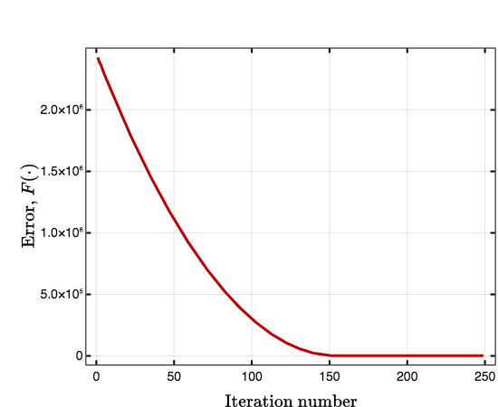
Figure 2: Objective function of the Bilevel problem, i.e., $F(\boldsymbol{\beta}_{j},{\mathbf{g}}_{j})$ as a function of the number of iterations $j$.

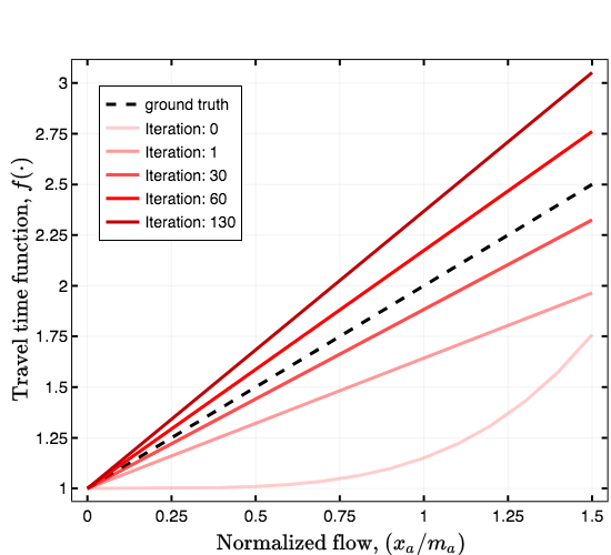
Figure 3: Cost function estimators with respect to the joint iterations. In this example, the cost function coefficient converges around iteration $j=130$.

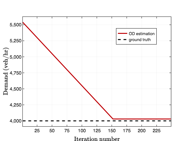
Figure 4: Demand estimator for OD pair $(1,2)$ with respect to the joint iterations.

V CONCLUSION

In this work, we were able to solve the joint problem of estimating OD demands and cost functions in a transportation network. We approached the problem by rewriting (9) with the lower-level KKT conditions (13). Then, we solved the problem using an iterative approach (14). To be able to accomplish this, we relaxed some constraints by allowing a small gap to exist between the primal-dual costs. Additionally, we took care of the non-convexity of the constraints by using the previous iteration solution and bounding these variables.

Finally, we tested our algorithm using the Braess network and concluded that our proposed method works well in terms of reducing the objective function of the bilevel formulation (9). We performed this task by adjusting both, the OD demand and the cost functions. It is important to keep in mind that the output of the algorithm is sensitive to the accuracy of flow observations and to the parameters chosen. To overcome the parameter selection issue, we suggest practitioners to use cross-validation techniques. As future extensions of this work, we plan to implement this algorithm in significantly larger networks and we aim at extending our framework to multi-class transportation networks.

References

- [1] D. K. Merchant and G. L. Nemhauser, “A model and an algorithm for the dynamic traffic assignment problems,” Transportation Science, vol. 12, no. 3, pp. 183–199, 1978.
- [2] M. Patriksson, “The Traffic Assignment Problem: Models and Methods,” Annals of Physics, vol. 54, no. 2, pp. xii, 223 p., 1994.
- [3] D. Bertsimas, V. Gupta, and I. C. Paschalidis, “Data-driven estimation in equilibrium using inverse optimization,” Mathematical Programming, vol. 153, no. 2, pp. 595–633, 2015.
- [4] H. J. Van Zuylen and L. G. Willumsen, “The most likely trip matrix estimated from traffic counts,” Transportation Research Part B: Methodological, vol. 14, no. 3, pp. 281–293, 1980.
- [5] M. L. Hazelton, “Estimation of origin-destination matrices from link flows on uncongested networks,” Transportation Research Part B: Methodological, vol. 34, no. 7, pp. 549–566, 2000.
- [6] H. Spiess, “A maximum likelihood model for estimating origin-destination matrices,” Transportation Research Part B: Methodological, vol. 21, no. 5, pp. 395 – 412, 1987.
- [7] C. B. Winnie Daamen, “Traffic simulation and data: Validation methods and applications,” CRC Press, vol. 978-1482228700, no. 1, 2014.
- [8] T. A. Manual, “Bureau of public roads,” US Department of Commerce, 1964.
- [9] J. Zhang, S. Pourazarm, C. G. Cassandras, and I. C. Paschalidis, “The price of anarchy in transportation networks by estimating user cost functions from actual traffic data,” 2016 IEEE 55th Conference on Decision and Control, CDC 2016, no. Cdc, pp. 789–794, 2016.
- [10] ——, “The Price of Anarchy in Transportation Networks: Data-Driven Evaluation and Reduction Strategies,” Proceedings of the IEEE, vol. 106, no. 4, 2018.
- [11] H. Yang, Q. Meng, and M. G. H. Bell, “Simultaneous estimation of the origin-destination matrices and travel-cost coefficient for congested networks in a stochastic user equilibrium,” Transportation Science, vol. 35, no. 2, pp. 107–123, 2001.
- [12] D. Braess, A. Nagurney, and T. Wakolbinger, “On a Paradox of Traffic Planning,” Transportation Science, vol. 39, no. 4, pp. 446–450, 2005.
- [13] M. J. Beckmann, C. B. McGuire, and C. B. Winsten, “Studies in the Economics of Transportation,” p. 359, 1955.
- [14] M. J. Smith, “The existence, uniqueness and stability of traffic equilibria,” Transportation Research Part B, vol. 13, no. 4, pp. 295–304, 1979.
- [15] S. Dafermos, “Traffic Equilibrium and Variational Inequalities,” Transportation Science, vol. 14, no. 1, pp. 42–54, 1980.
- [16] C. F. Daganzo and Y. Sheffi, “On stochastic models of traffic assignment,” Transportation Science, vol. 11, no. 3, pp. 253–274, 1977.
- [17] M. Patriksson, “Sensitivity analysis of traffic equilibria,” Transportation Science, vol. 38, no. 3, pp. 258–281, Aug. 2004.
- [18] R. Tobin and T. Friesz, “Sensitivity analysis for equilibrium network flow,” Transportation Science, vol. 22, no. 4, pp. 242–250, 1 1988.
- [19] M. Josefsson and M. Patriksson, “Sensitivity analysis of separable traffic equilibrium equilibria with application to bilevel optimization in network design,” Transportation Research Part B: Methodological, vol. 41, no. 1, pp. 4 – 31, 2007.