Drag force on heavy quarks from holographic QCD

Abstract

We study the drag force of a relativistic heavy quark using a holographic QCD model with conformal invariance broken by a background dilaton. We analyze the effects of chemical potential and confining scale on this quantity, respectively. It is shown that the drag force in this model is larger than that of $\mathcal{N}=4$ supersymmetric Yang-Mills (SYM) plasma. In particular, the inclusion of the chemical potential and confining scale both enhance the drag force, in agreement with earlier findings. Also, we discuss how chemical potential and confining scale influence the diffusion coefficient.

I Introduction

The ultra-relativistic heavy-ion experimental programs at the Relativistic Heavy Ion Collider (RHIC) and the Large Hadron Collider (LHC) have created a new type of matter so-called quark gluon plasma (QGP) EV ; KA ; JA . One of the interesting features of QGP is jet quenching (parton energy loss): high energy partons propagate through the hot and dense medium, they interact with the medium and hence lose energy. Usually, the jet quenching phenomenon could be characterized by the jet quenching parameter, defined by the average transverse momentum square transferred from the traversing parton, per unit mean free path XN . Alternately, this phenomenon could be studied from the drag force: heavy quarks move through the QGP, they feel a drag force and hence lose energy. In weakly coupling theories, the jet quenching has already been investigated in many works BG0 ; RB2 ; RB1 ; UA ; AMY ; SJ ; GLV . However, a lot of experiments find strong evidence that QGP does not behave as a weakly coupled gas, but rather as a strongly coupled fluid. Consequently, calculational techniques for strongly coupled, real-time QCD dynamics are required. Such techniques are now available via the gauge/gravatity duality or AdS/CFT correspondence Maldacena:1997re ; MadalcenaReview ; Gubser:1998bc .

AdS/CFT, a conjectured duality between a string theory in the AdS space and a conformal field theory on the AdS space boundary, has yielded lots of important insights for exploring various aspects of QGP JCA . In the frame work of AdS/CFT, the drag force of a heavy quark moving in $\mathcal{N}=4$ SYM plasma was proposed in GB ; CP . Therein, this force could be related to the damping rate $u$ (or called friction coefficient), defined by the Langevin equation, $dp/dt=-up+f$, subject to a driving force $f$. For $dp/dt=0$, i.e., constant speed trajectory, $f$ equals to the drag force. It was found that CP ; GB

$$f_{SYM}=-\frac{\pi\sqrt{\lambda}T^{2}}{2}\frac{v}{\sqrt{1-v^{2}}},$$ (1)

where $v$, $T$, $\lambda$ are the quark velocity, the plasma temperature and ’t Hooft coupling, respectively. Subsequently, this idea has been generalized to various cases, such as chemical potential ECA ; SCH ; LC , finite coupling KBF , non-commutativity plasma TMA and AdS/QCD models PE ; ENA ; UGU . Other studies in this direction can be found in OA0 ; ZQ ; DGI ; KLP ; ANA ; MCH ; SRO ; SSG1 ; JSA .

In this paper we study the drag force in a soft wall-like model, i.e., the SW_T,μ model, which is motivated by the soft wall model of AKE . The SW_T,μ model was proposed in PCO to investigate the heavy quark free energy and the QCD phase diagram. It was shown that such a model provides a nice phenomenological description of quark-antiquark interaction as well as some hadronic properties. Recently, the authors of zq investigated the imaginary potential in this model and found that the presence of the confining scale tends to reduce the quarkonia dissociation, reverse to the effect of the chemical potential. Also, there are other investigations of models of this type OA1 ; CPA ; PCO2 ; PCO1 ; XCH ; CE . Motivated by this, here we consider the drag force in this model and understand the possible physical implications of our results in this dual plasma. Another motivation for this paper is that previous works either discuss the drag force in some strongly coupled thermal gauge theories (not holographic QCD) with chemical potential ECA ; SCH ; LC or holographic QCD without chemical potential ENA ; PE ; UGU . Here we give such analysis in holographic QCD with chemical potential.

The structure of this paper is as follows. In the next section, we introduce the geometry of the SW_T,μ model given in PCO . In section 3 and section 4, we analyze the behavior of the drag force and the diffusion coefficient for the SW_T,μ model, in turn. Summary and discussions are given in the final section.

II Setup

To begin with, we introduce the holographic models in terms of the action OD

$$S=\frac{1}{16\pi G_{5}}\int d^{5}x\sqrt{-g}(\mathcal{R}-\frac{1}{2}\partial_{M}\phi\partial^{M}\phi-V(\phi)-\frac{f(\phi)}{4}F_{MN}F^{MN}),$$ (2)

where $G_{5}$ is the five-dimensional (5D) Newton constant. $g$ stands for the determinant of the metric $g_{MN}$. $\mathcal{R}$ represents the Ricci scalar. $\phi$ denotes the scalar which induces the deformation away from conformality. $V(\phi)$ refers to the potential which contains the cosmological constant and some other terms. $F_{MN}$ and $f(\phi)$ are the field strength tensor and gauge kinetic function, respectively.

For (2), the equations of motion are

$$\mathcal{R}_{MN}-\frac{1}{2}\mathcal{R}g_{MN}=T_{MN},$$ (3)

$$\nabla_{M}(f(\phi)F^{MN})=0,$$ (4)

$$\nabla^{M}\nabla_{M}\phi=V^{\prime}(\phi)+\frac{f^{\prime}(\phi)}{4}F_{MN}F^{MN},$$ (5)

with

$$T_{MN}=\frac{1}{2}[f(\phi)(F_{MA}F_{N}^{A}-\frac{1}{4}g_{MN}F_{AB}F^{AB})+(\partial_{M}\phi\partial_{N}\phi-\frac{1}{2}g_{MN}\partial_{A}\phi\partial^{A}\phi)-g_{MN}V(\phi)],$$ (6)

where $\nabla_{M}$ represents the Levi-Civita covariant derivative related to $g_{MN}$.

Notice that with $\phi=0$, the AdS black hole arises as a solution of (3)-(6). Next, by considering a non-vanishing gauge-field component $A_{0}$ with the conditions

$$A_{0}(z=0)=\mu R,\qquad A_{0}(z_{0}=z_{h})=0,$$ (7)

and solving (3)-(6), one can obtain the AdS-RN spacetime, whose metric is given by

$$ds^{2}=\frac{R^{2}}{z^{2}}(-f(z)dt^{2}+d\vec{x}^{2}+\frac{dz^{2}}{f(z)}),$$ (8)

with

$$f(z)=1-(1+Q^{2})\frac{z^{4}}{z_{h}^{4}}+Q^{2}\frac{z^{6}}{z_{h}^{6}},\qquad Q=\mu z_{h}/\sqrt{3}$$ (9)

where $R$ is the AdS radius. $Q$ denotes the black hole charge, constrained in $0\leq Q\leq\sqrt{2}$. $z$ stands for the 5th coordinate with $z=z_{h}$ the horizon and $z=0$ the boundary. $\mu$ represents the chemical potential. Note that the chemical potential implemented here is not the quark (or baryon) chemical potential of QCD but a chemical potential corresponding to the R-charge of $\mathcal{N}=4$ SYM. Nevertheless, it could serve as a simple way of introducing finite density effects into the system.

Moreover, the temperature of the black hole is

$$T=\frac{1}{\pi z_{h}}(1-\frac{Q^{2}}{2}).$$ (10)

Explicitly, for given $(T,\mu)$ in the boundary theory, $(z_{h},Q)$ of the bulk theory can be expressed as

$$z_{h}(T,\mu)=\frac{3\pi T}{\mu^{2}}[\sqrt{1+\frac{2}{3\pi^{2}}(\frac{\mu}{T})^{2}}-1],$$ (11)

$$Q(T,\mu)=\frac{\sqrt{3}\pi T}{\mu}[\sqrt{1+\frac{2}{3\pi^{2}}(\frac{\mu}{T})^{2}}-1].$$ (12)

To emulate confinement in the boundary theory at vanishing temperature, one can introduce a warp factor to the background, similar to OA1 . Then the metric of the SW_T,μ model is given by PCO

$$ds^{2}=\frac{R^{2}}{z^{2}}h(z)(-f(z)dt^{2}+d\vec{x}^{2}+\frac{dz^{2}}{f(z)}),\qquad h(z)=e^{c^{2}z^{2}},$$ (13)

where $c$ is deformation parameter (related to the confining scale) which has the dimension of energy. Here we will not focus on a specific model, but rather study the behavior of the drag force in a class of models parametrized by $c$. So we will make $c$ dimensionless by normalizing it to fixed temperatures and express other quantities in units of $c$. In Ref HLL , it was shown that the range of $0\leq c/T\leq 2.5$ may be most relevant for a comparison with QCD. We will use this range here.

To proceed, if one uses $r=R^{2}/z$ as the radial coordinate, then metric (13) turns into

$$ds^{2}=\frac{r^{2}h(r)}{R^{2}}(-f(r)dt^{2}+d\vec{x}^{2})+\frac{R^{2}h(r)}{r^{2}f(r)}dr^{2},$$ (14)

with

$$f(r)=1-(1+Q^{2})(\frac{r_{h}}{r})^{4}+Q^{2}(\frac{r_{h}}{r})^{6},\qquad h(r)=e^{\frac{c^{2}R^{4}}{r^{2}}},$$ (15)

now $T=\frac{r_{h}}{\pi R^{2}}(1-\frac{Q^{2}}{2})$, $\mu=\frac{\sqrt{3}Qr_{h}}{R^{2}}$. The horizon and boundary are $r=r_{h}$ and $r=\infty$, respectively. It should be noticed that metric (13) and metric (14) are equivalent but with different coordinate systems.

III drag force

In this section, we will follow the argument in GB ; CP to analyze the drag force in the SW_T,μ model. The string dynamic is described by the Nambu-Goto action, given by

$$S=-\frac{1}{2\pi\alpha^{\prime}}\int d\tau d\sigma\sqrt{-g},$$ (16)

with $g$ the determinant of the induced metric and

$$g_{\alpha\beta}=g_{\mu\nu}\frac{\partial X^{\mu}}{\partial\sigma^{\alpha}}\frac{\partial X^{\nu}}{\partial\sigma^{\beta}},$$ (17)

with $g_{\mu\nu}$ the brane metric and $X^{\mu}$ the target space coordinates.

One considers a heavy quark moving with constant speed $v$ in one direction, (e.g., the $x_{1}$ direction) and takes the gauge

$$t=\tau,\qquad x_{1}=vt+\xi(r),\qquad x_{2}=0,\qquad x_{3}=0,\qquad r=\sigma,$$ (18)

then the induced metric can be obtained by plugging (18) into (14),

$$g_{tt}=-\frac{r^{2}f(r)h(r)}{R^{2}},\qquad g_{xx}=\frac{r^{2}h(r)}{R^{2}},\qquad g_{rr}=\frac{R^{2}h(r)}{r^{2}f(r)}.$$ (19)

Given that, the Lagrangian density reads

$$\mathcal{L}=\sqrt{-g_{rr}g_{tt}-g_{rr}g_{xx}v^{2}-g_{xx}g_{tt}{\xi^{\prime}}^{2}}=h(r)\sqrt{[1-\frac{v^{2}}{f(r)}+\frac{r^{4}f(r)}{R^{4}}{\xi^{\prime}}^{2}]},$$ (20)

with $\xi^{\prime}=d\xi/d\sigma$. As the action does not depend on $\xi$ explicitly, the energy-momentum current $\Pi_{\xi}$ is a constant,

$$\Pi_{\xi}=\frac{\partial\mathcal{L}}{\partial\xi^{\prime}}=\xi^{\prime}\frac{h(r)r^{4}f(r)/R^{4}}{\sqrt{1-\frac{v^{2}}{f(r)}+\frac{r^{4}f(r)}{R^{4}}{\xi^{\prime}}^{2}}}=constant,$$ (21)

yielding

$$\xi^{\prime}=\frac{\Pi_{\xi}R^{2}}{r^{2}f(r)}\sqrt{\frac{f(r)-v^{2}}{r^{4}h^{2}(r)f(r)/R^{4}-{\Pi_{\xi}}^{2}}},$$ (22)

where $\xi^{\prime}$ can be regarded as the configuration of string tail.

Near the horizon $r_{h}$, the denominator and numerator (inside the square root of Eq.(22)) are negative for small $r$ and positive for large $r$. Also, the ratio should be positive. Under these conditions, one gets that the numerator and denominator should change sigh at the same point (namely $r_{c}$). For the numerator, one gets

$$f(r_{c})=v^{2},$$ (23)

results in

$$Q^{2}(\frac{r_{h}}{r_{c}})^{6}-(1+Q^{2})(\frac{r_{h}}{r_{c}})^{4}+1-v^{2}=0,$$ (24)

note that for given values of $Q$ and $v$, the analytic expressions of $r_{h}/r_{c}$ can be determined from Eq.(24) but these are cumbersome and not very illuminating. Here we will mainly focus on the numerical results.

The denominator also changes sign at $r_{c}$, yielding

$${\Pi_{\xi}}=\frac{r_{c}^{2}h(r_{c})\sqrt{f(r_{c})}}{R^{2}},$$ (25)

with

$$h(r_{c})=e^{\frac{c^{2}R^{4}}{r_{c}^{2}}}.$$ (26)

On the other hand, the current density reads

$$\pi_{x}^{r}=-\frac{1}{2\pi\alpha^{\prime}}\xi^{\prime}\frac{g_{tt}g_{xx}}{-g},$$ (27)

and the drag force reads

$$f=\frac{dp_{1}}{dt}=\sqrt{-g}\pi_{x}^{r},$$ (28)

where the minus indicates that the drag force is against the direction of motion, as expected.

Next, applying the relations

$$\lambda=g_{YM}^{2}N_{c}=\frac{R^{4}}{{\alpha^{\prime}}^{2}},\qquad T=\frac{r_{h}}{\pi R^{2}}(1-\frac{Q^{2}}{2}),$$ (29)

one arrives at the drag force in the SW_T,μ model

$$f=-\frac{\pi T^{2}\sqrt{\lambda}}{2}\frac{vh(r_{c})}{(1-\frac{Q^{2}}{2})^{2}(\frac{r_{h}}{r_{c}})^{2}}.$$ (30)

Notice that by taking $Q=0$ (or $\mu=0$, which gives $(\frac{r_{h}}{r_{c}})^{2}=\sqrt{1-v^{2}}$) and $c=0$ (corresponding to $h(r_{c})=1$) in Eq.(30), the results of $\mathcal{N}=4$ SYM GB ; CP are recovered.

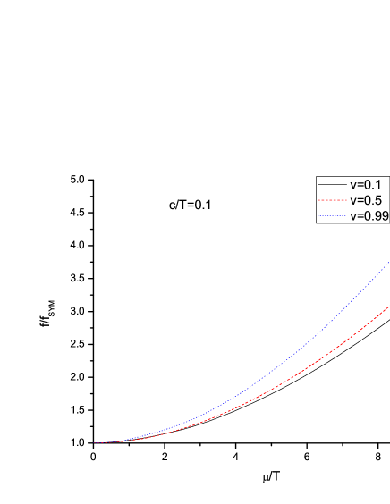
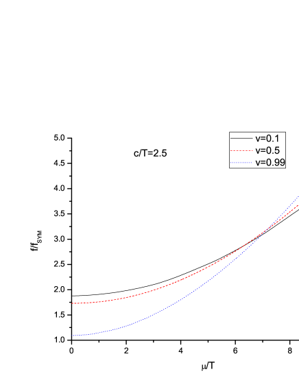
Figure 1: $f/f_{SYM}$ versus $\mu/T$. Here we take the speed of light as unit.

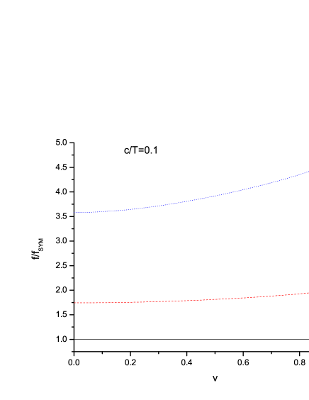
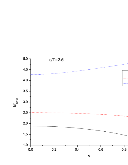
Figure 2: $f/f_{SYM}$ versus $v$. Here we take the speed of light as unit.

To proceed, we compare the drag force in the SW_T,μ model with its counterpart of the $\mathcal{N}=4$ SYM as the following

$$\frac{f}{f_{SYM}}=\frac{h(r_{c})\sqrt{1-v^{2}}}{(1-\frac{Q^{2}}{2})^{2}(\frac{r_{h}}{r_{c}})^{2}}.$$ (31)

In fig.1, we plot $f/f_{SYM}$ against $\mu/T$ for two fixed values of $c/T$. The left panel is for $c/T=0.1$ and the right one is for $c/T=2.5$. From these figures, one sees that the drag force in the SW_T,μ model is larger than that of $\mathcal{N}=4$ SYM plasma. Also, increases $\mu/T$ leads to increasing the drag force. Namely, the chemical potential enhances the drag force, consistently with ECA ; SCH ; LC . In addition, by comparing the two panels, one finds that increasing $c/T$ increases the drag force. Thus, one concludes that the confining scale also enhances the drag force, in accordance with ENA .

In fig.2, we plot $f/f_{SYM}$ versus $v$ for various cases. From the left panel (small $c/T$ case), one finds that increasing $v$ enhances $f$, especially this effect is more pronounced for large $\mu/T$. But the right panel (large $c/T$ case) is different: for small $\mu/T$, $f/f_{SYM}$ decreases with $v$ but for large $\mu/T$ the situation reverses. Interestingly, a similar non-monotone behavior appears in the studies of the drag force with curvature-squared corrections KBF .

Also, one could analyze the effect of $c$ and $\mu$ on the viscosity. As we know, a stronger force implies a more strongly coupled medium, closer to an ideal liquid. As the drag force in the SW_T,μ model is larger than that of $\mathcal{N}=4$ SYM, one could infer that the plasma is less viscous in the SW_T,μ model than in $\mathcal{N}=4$ SYM plasma.

Before closing this section, we would like to mention that Ref OA0 has studied the drag force in the soft wall model and estimated the spatial string tension at finite $T$ and $\mu$ recently.

IV diffusion coefficient

In this section, we investigate the behavior of the diffusion coefficient in the SW_T,μ model. First, we remember the results of $\mathcal{N}=4$ SYM. The drag force is given by

$$f_{SYM}=\frac{dp_{1}}{dt}=-\frac{\pi T^{2}\sqrt{\lambda}}{2}\frac{v}{\sqrt{1-v^{2}}}.$$ (32)

Assuming $p_{1}=mv/\sqrt{1-v^{2}}$, Eq.(37) becomes

$$\frac{dp_{1}}{dt}=-\frac{\pi T^{2}\sqrt{\lambda}}{2}\frac{p_{1}}{m}.$$ (33)

Integrating (33), one obtains

$$p_{1}(t)=p_{1}(0)e^{-t/t_{SYM}},\qquad t_{SYM}=\frac{2m}{\pi T^{2}\sqrt{\lambda}},$$ (34)

where $t_{SYM}$ is the relaxation time of $\mathcal{N}=4$ SYM.

On the other hand, the diffusion coefficient is related to the temperature, the heavy quark mass and the relaxation time as GB ; CP

$$D=\frac{T}{m}t_{D}.$$ (35)

Using the above approach, one readily gets

$$D_{SYM}=\frac{2}{\pi T\sqrt{\lambda}}.$$ (36)

Likewise, from (30) one can rewrite the drag force in the SW_T,μ as

$$f=-\frac{\pi p_{1}T^{2}\sqrt{\lambda}}{2m}\frac{\sqrt{(1-v^{2})}h(r_{c})}{(1-\frac{Q^{2}}{2})^{2}(\frac{r_{h}}{r_{c}})^{2}}.$$ (37)

In a similar manner, one arrives at the diffusion coefficient in the SW_T,μ model

$$D=\frac{T}{m}t_{D}=-\frac{T}{m}\frac{p_{1}}{f}=\frac{(1-\frac{Q^{2}}{2})^{2}(\frac{r_{h}}{r_{c}})^{2}}{h(r_{c})\sqrt{1-v^{2}}}\frac{2}{\pi T\sqrt{\lambda}}.$$ (38)

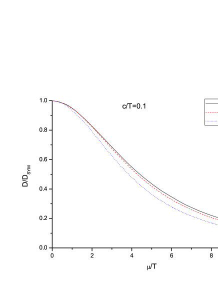
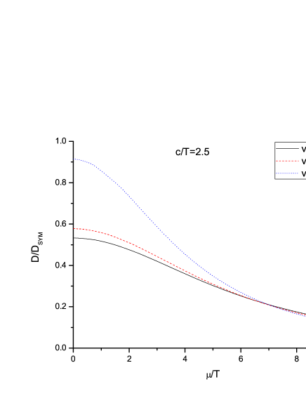
Figure 3: $D/D_{SYM}$ versus $\mu/T$. Here we take the speed of light as unit

In fig.3, we plot $D/D_{SYM}$ as a function of $\mu/T$ . One can see that $\mu$ and $c$ both reduce the diffusion coefficient.

Also, the inclusion of $\mu$ and $c$ may influence the heavy quark mass. As discussed in JCAS , the relaxation time $t_{D}=\frac{m}{T}D$ should be larger than the inverse temperature

$$t_{D}>>\frac{1}{T},$$ (39)

yielding

$$m>>\frac{h(r_{c})\sqrt{1-v^{2}}}{(1-\frac{Q^{2}}{2})^{2}(\frac{r_{h}}{r_{c}})^{2}}\frac{\pi T\sqrt{\lambda}}{2},$$ (40)

one can see that $\mu$ and $c$ may enhance the heavy quark mass.

V Conclusion

In this work, we studied the drag force and diffusion coefficient in a soft wall model with finite temperature and chemical potential. Our goal is to understand the interplay between the presence of confining scale (so the plasma is not conformal) and the chemical potential (the QGP is assumed to carry a finite, albeit small, baryon number density) when estimating the drag force of a heavy quark in a strongly coupled plasma. It is shown that with fixed $c$ the presence of $\mu$ increases the drag force and decreases the diffusion coefficient, in agreement with the findings of ECA ; SCH ; LC . Also, with fixed $\mu$ the inclusion of $c$ increases the drag force as well, in accordance with ENA . Therefore, our results ($\mu$ and $c$ existed at the same time) confirm the results of $\mu$ or $c$ stands alone. On the other hand, the results show that the plasma is less viscous in the SW_T,μ model than in $\mathcal{N}=4$ SYM.

However, it should be admitted that the SW_T,μ model consider here has several drawbacks. First, it is not a consistent model since it does not solve the Einstein equations. It would be interesting to give such analysis in some consistent models, e.g. ja ; dl ; RCR ; SH ; DL0 (generally, the metrics of those models are only known numerically, so the calculates are quite challenging. Also, in these models the dilaton field would be non-trivial, so the coupling of the dilaton to the word-sheet should be taken into account UG1 ; JNO ; MM ). Moreover, the SW_T,μ model may miss a part about the phase transition, since Refs DL ; RG2 ; FZ ; FZ1 argued that there may be a first order phase transition if one sets the warp factor to be $cz^{2}$ and solves the equation of motion self-consistently. It would be significant to consider these effects.

Finally, it is also of interest to study the jet quenching parameter HLI and stopping distance PMC ; SSG ; PAR in the SW_T,μ model and compare with the results of this work. We leave this as a further study.

VI Acknowledgments

We would like to extend our gratitude to Dr. Zi-qiang Zhang for helpful and encouraging discussions. This work is supported by Guizhou Provincial Key Laboratory Of Computational Nano-Material Science under Grant No. 2018LCNS002.

References

- (1) E. V. Shuryak, Nucl. Phys. A 750, 64 (2005).
- (2) K. Adcox et al. [PHENIX Collaboration], Nucl. Phys. A 757, 184 (2005).
- (3) J. Adams et al. [STAR Collaboration], Nucl. Phys. A 757, 102 (2005).
- (4) X. N. Wang and M. Gyulassy, Phys. Rev. Lett. 68, 1480 (1992).
- (5) B. G. Zakharov, JETP Lett. 63, 952 (1996).
- (6) R. Baier, Y. L. Dokshitzer, A. H. Mueller and D. Schiff, JHEP 09 (2001) 033.
- (7) R. Baier, Y. L. Dokshitzer, A. H. Mueller, S. Peigne and D. Schiff, Nucl. Phys. B 484, 265 (1997).
- (8) U. A. Wiedemann, Nucl. Phys. B 588, 303 (2000).
- (9) P. Arnold, G. D. Moore and L. G. Yaffe, JHEP 11 (2001) 057.
- (10) S. Jeon and G.D. Moore, Phys. Rev. D 71 (2005) 034901.
- (11) M. Gyulassy, P. Levai and I. Vitev, Phys. Rev. Lett. 85, 5535 (2000).
- (12) J. M. Maldacena, Adv. Theor. Math. Phys. 2, 231 (1998).
- (13) O. Aharony, S. S. Gubser, J. Maldacena, H. Ooguri and Y. Oz, Phys. Rept. 323, 183 (2000).
- (14) S. S. Gubser, I. R. Klebanov and A. M. Polyakov, Phys. Lett. B 428, 105 (1998).
- (15) J. C. Solana, H. Liu, D. Mateos, K. Rajagopal and U. A. Wiedemann, arXiv:1101.0618
- (16) C. P. Herzog, A. Karch, P. Kovtun, C. Kozcaz and L. G. Yafe, JHEP 07 (2006) 013.
- (17) S. S. Gubser, Phys. Rev. D 74 (2006) 126005.
- (18) E. Caceres and A. Guijosa, JHEP 11 (2006) 077.
- (19) S. Chakraborty and N. Haque, JHEP 12 (2014) 175.
- (20) L. Cheng, X.-H. Ge and S.-Y. Wu, Eur. Phys. J. C 76 256 (2016).
- (21) K. B. Fadafan, JHEP 12 (2008) 051.
- (22) T. Matsuo, D. Tomino and W.-Y. Wen, JHEP 10 (2006) 055.
- (23) P. Talavera, JHEP 01 (2007) 086.
- (24) E. Nakano, S. Teraguchi and W.-Y. Wen, Phys. Rev. D 75 (2007) 085016.
- (25) U. Gursoy, E. Kiritsis, G. Michalogiorgakis and F. Nitti, JHEP 12 (2009) 056.
- (26) O. Andreev, Phys. Rev. D 98 (2018) 066007.
- (27) Z.-q. Zhang, K. Ma, D.-f. Hou, J. Phys. G: Nucl. Part. Phys. 45 (2018) 025003.
- (28) D. Giataganas, JHEP 07 (2012) 031.
- (29) K. L. Panigrahi and S. Roy, JHEP 04 (2010) 003.
- (30) A. N. Atmaja and K. Schalm, JHEP 04 (2011) 070.
- (31) M. Chernicoff, D. Fernandez, D. Mateos and D. Trancanelli, JHEP 1208 (2012) 100.
- (32) S. Roy, Phys. Lett. B 682, 93 (2009).
- (33) S. S. Gubser, Phys. Rev. D 76 (2007) 126003.
- (34) J. Sadeghi, M. R. Setare, B. Pourhassan and S. Hashmatian, Eur. Phys. J. C 61 527 (2009).
- (35) A. Karch, E. Katz, D. T. Son and M. A. Stephanov, Phys. Rev. D 74, 015005 (2006).
- (36) P. Colangelo, F. Giannuzzi, and S. Nicotri, Phys. Rev. D 83 (2011) 035015.
- (37) Z.-q. Zhang and X.R. Zhu, Phys. Lett. B 793 (2019) 200-205.
- (38) O. Andreev, Phys. Rev. D 81 (2010) 087901 .
- (39) C. Park, D.-Y. Gwak, B.-H. Lee, Y. Ko and S. Shin, Phys. Rev. D 84 (2011) 046007.
- (40) P. Colangelo, F. Giannuzzi, S. Nicotri and F. Zuo, Phys. Rev. D 88 (2013) 115011.
- (41) P. Colangelo, F. Giannuzzi and S. Nicotri, JHEP 05 (2012) 076.
- (42) X. Chen, S.-Q. Feng, Y.-F. Shi, Y. Zhong, Phys. Rev. D 97 (2018) 066015.
- (43) C. Ewerz, T. Gasenzer, M. Karl, and A. Samberg, JHEP 05 (2015) 070.
- (44) O. DeWolfe, S. S. Gubser, and C. Rosen, Phys. Rev. D 83 (2011) 086005.
- (45) O. Andreev and V. I. Zakharov, Phys. Lett. B 645, 437 (2007).
- (46) H. Liu, K. Rajagopal and Y. Shi, JHEP 08 (2008) 048.
- (47) J. C. Solana and D. Teaney, Phys. Rev. D 74 (2006) 085012.
- (48) A. Stoffers and I. Zahed, Phys. Rev. D 83 (2011) 055016.
- (49) R. Rougemont, A. Ficnar, S. Finazzo, and J. Noronha, JHEP 1604 (2016) 102.
- (50) R. Critelli, J. Noronha, J. N.-Hostler, I. Portillo, C. Ratti and R. Rougemont, Phys. Rev. D 96, 096026 (2017).
- (51) S. He, S.-Y. Wu, Y. Yang, and P.-H. Yuan, JHEP 04 (2013) 093.
- (52) D. n. Li, M. Huang, JHEP 11 (2013) 088.
- (53) U. Gursoy, E. Kiritsis, F. Nitti, JHEP 02 (2008) 019.
- (54) J. Noronha. Phys.Rev. D 81 (2010) 045011.
- (55) M. Mia, K. Dasgupta, C. Gale, S. Jeon, Phys.Rev. D82 (2010) 026004.
- (56) D. n. Li, S. He, M. Huang, Q. s. Yan, JHEP 09 (2011) 041.
- (57) R. G. Cai, S. He, D. n. Li, JHEP 03 (2012) 033.
- (58) F. Zuo, Y. H. Gao, JHEP 07 (2014) 147.
- (59) F. Zuo, JHEP 06 (2014) 143.
- (60) H. Liu, K. Rajagopal and U. A. Wiedemann, Phys. Rev. Lett. 97, 182301 (2006).
- (61) P. M. Chesler, K. Jensen, A. Karch and L. G. Yaffe, Phys. Rev. D 79 (2009) 125015.
- (62) S. S. Gubser, D. R. Gulotta, S. S. Pufu and F. D. Rocha, JHEP 10 (2008) 052.
- (63) P. Arnold and D. Vaman, JHEP 10 (2010) 099.