Efficiency of Coordinate Descent Methods For Structured Nonconvex Optimization

Abstract

Novel coordinate descent (CD) methods are proposed for minimizing nonconvex functions consisting of three terms: (i) a continuously differentiable term, (ii) a simple convex term, and (iii) a concave and continuous term. First, by extending randomized CD to nonsmooth nonconvex settings, we develop a coordinate subgradient method that randomly updates block-coordinate variables by using block composite subgradient mapping. This method converges asymptotically to critical points with proven sublinear convergence rate for certain optimality measures. Second, we develop a randomly permuted CD method with two alternating steps: linearizing the concave part and cycling through variables. We prove asymptotic convergence to critical points and sublinear complexity rate for objectives with both smooth and concave parts. Third, we extend accelerated coordinate descent (ACD) to nonsmooth and nonconvex optimization to develop a novel randomized proximal DC algorithm whereby we solve the subproblem inexactly by ACD. Convergence is guaranteed with at most a few number of ACD iterations for each DC subproblem, and convergence complexity is established for identification of some approximate critical points. Fourth, we further develop the third method to minimize certain ill-conditioned nonconvex functions: weakly convex functions with high Lipschitz constant to negative curvature ratios. We show that, under specific criteria, the ACD-based randomized method has superior complexity compared to conventional gradient methods. Finally, an empirical study on sparsity-inducing learning models demonstrates that CD methods are superior to gradient-based methods for certain large-scale problems.

1 Introduction

Coordinate descent (CD) methods update only a subset of coordinate variables in each iteration, keeping other variables fixed. Due to their scalability to the so-called “big data” problems (see [26, 22, 17, 27, 4]), CD methods have attracted significant attention from machine learning and data science. This paper will develop efficient CD methods for large-scale structured nonconvex problems in the following form:

x∈R^dF(x)=f(x)+ϕ(x) - h(x), where $f(x)$ is continuously differentiable, $\phi(x)$ is convex lower-semicontinuous with a simple structure, and $h(x)$ is convex continuous. The nonconvex problem formed in (1) is sufficiently powerful to express a variety of machine learning applications, including sparse regression, low rank optimization, and clustering (see [33, 18, 29]).

Our main contribution to the field is that we propose a number of novel CD methods with guaranteed convergence for a broad class of nonconvex problems described by (1). Our methods include extending RCD and cyclic CD to nonsmooth and nonconvex settings, and new randomized proximal DC and proximal point methods by using ACD to solve the subproblems. For all the proposed algorithms, we not only provide guarantees to asymptotic convergence, but also prove rate of convergence for properly defined optimality measures. To the best of our knowledge, this is the first study of coordinate descent methods for such nonsmooth and nonconvex optimization with complexity efficiency guarantee. Our results are summarized as follows.

Our first result is a new randomized coordinate subgradient descent (RCSD) method for nonsmooth nonconvex and composite problems. While our algorithm recovers existing nonconvex CD methods [25] as a special case, it allows the nonsmooth part to be inseparable and concave, and coordinates to be sampled either uniformly or non-uniformly at random. We show the asymptotic convergence to critical points, and we establish the sublinear rate of convergence for a proposed optimality measure which naturally extends the proximal gradient mapping to nonsmooth and nonconvex settings.

Motivated by block coordinate gradient descent (BCGD) [4], we propose a new randomly permuted coordinate descent (RPCD) for nonsmooth and nonconvex optimization. Our primary innovation is to alternate RPCD between linearizing the concave part $h(x)$ and successively updating all the block-coordinate variables based on some cycling order. The cycling order can be either deterministic or randomly shuffled, provided that each block of variables is updated once in each loop. We provide asymptotic convergence of BCGD method to critical points. For a certain case ($\phi(x)=0$), we also establish a sublinear rate of convergence of the subgradient norm.

We next extend accelerated coordinate descent methods to the nonsmooth and nonconvex setting by considering the difference-of-convex representation of Problem (1). We propose an ACD-based proximal DC (ACPDC) algorithm by transforming $F(x)$ into a sequence of strongly convex functions that are approximately minimized by the ACD method. We show that ACPDC is sufficiently fast that only a few rounds of ACD are needed in each iteration. Hence, ACPDC offers significant improvements compared to the classic DC algorithm, which requires exact optimal solutions to the subproblems. ACPDC also offers advantages to the proximal DC algorithm, an extension of the DC algorithm that performs one proximal gradient descent step to minimize the majorized function. Taking advantages of the fast convergence of ACD, ACPDC is more efficient than gradient-based DC algorithm in exploiting the problem structure, offering a much better trade-off between iteration complexity and running time.

Finally, we draw attention to minimization of weakly convex functions, namely, the nonconvex functions with bounded negative curvature, and propose a new ACD-based proximal point method (ACPP) for solving such problems. By assuming that the objective function is weakly convex, faster rates of convergence can be attained. Specifically, we show that the complexity rate of ACPP can be significantly better than that of classic CD approaches for ill-conditioned problems; ill-conditioned problems are those that have a relatively high ratio between Lipschitz constant to negative curvature.

Related work

There is a significant body of work on CD methods for nonconvex optimization. We refer to [17] for some general strategies to develop block update algorithms for nonconvex optimization. [32] proposed proximal cyclic CD methods for minimizing composite functions with nonconvex separable regularizers. However, their work didn’t include the nonconvex and nonsmooth function described in (1). See such an example in Section 7. A recent work [16] extended the cyclic block mirror descent to the nonsmooth setting, and guaranteed asymptotic convergence to block-wise optimality for minimizing Problem (1). In contrast, our work directly guarantees convergence to the critical points by employing a different linearization technique to handle the nonsmooth part $h(x)$. The work [3] proposed efficient CD-type algorithms for achieving specific coordinate-wise optimality for problems with group sparsity terms; they proved that the proposed coordinate-wise optimality is more restrictive than stationarity for such nonconvex problems. Apart from these works, a number of CD methods with complexity guarantees have also been developed. For example, [25] proposed randomized coordinate descent for nonconvex composite problems, possibly with a linear constraint. Their algorithm 1-RCD can be viewed as a special case of our first algorithm RCSD when $h(x)$ is void and uniform sampling is adopted. Additionally, [7] proposed randomized block mirror descent for stochastic optimization of convex and nonconvex composite problems. However, none of these proposals consider a concave nonsmooth part in the objective, nor do they improve on algorithm efficiency for the ill-conditioned nonconvex problem; we fully address both of these challenges for coordinate descent methods in this paper.

Another research line relevant to our study is the so-called DC optimization (see [28, 34, 33, 29]). Specified for minimizing the difference-of-convex (DC) functions, a DC algorithm alternates between linearizing the concave part and optimizing some convex surrogate of DC function by applying convex algorithms. Lately, much progress has been made in developing more efficient DC algorithms and in applying DC algorithms to machine learning and statistics (see [33, 18, 30, 31, 24]). We refer to the recent work [28] for a general review of DC algorithms and the applications. Notably, as a special case of DC functions, the weakly convex function has been increasingly popular due to its importance in machine learning and statistics ([12, 35, 9]). While it is possible to optimize weakly convex functions by directly generalizing convex methods to the nonconvex settings (see [13, 14, 25, 7]), much stronger efficiency guarantees can be obtained by indirect approaches such as proximal point methods and prox-linear methods (see [20, 19, 5, 8, 11, 9]). However, for the weakly-convex and the more general DC problems, it remains to develop efficient CD-type methods that are scalable to high-dimensional and large-scale data.

Outline of the paper

Section 2 introduces notations and preliminaries. Section 3 and Section 4 present RCSD and RPCD for nonsmooth nonconvex optimization, and then establish their convergence results. Section 5 presents a new DC algorithm based on ACD and demonstrates its asymptotic convergence to critical points and its convergence complexity of a proposed optimality measure. Section 6 considers the nonconvex problem with bounded negative curvature and presents an even faster proximal point algorithm based on using ACD. Section 7 discusses the applications of proposed methods on sparsity-inducing machine learning models, and present preliminary experiments to demonstrate the advantages of our proposed CD methods. Finally, Section 8 draws conclusions.

2 Notations and Preliminaries

We denote $[m]=\left\{1,2,...,m\right\}$. Let $d$ be a positive integer and $\mathbf{I}_{d}$ be the $d\times d$ identity matrix. Assume that matrix $\mathbf{U}_{i}\in\mathbb{R}^{d\times d_{i}}$ ($i\in[m]$) satisfies: $\left[\mathbf{U}_{1},\mathbf{U}_{2},...,\mathbf{U}_{m}\right]=\mathbf{I}_{d}$ where $\sum_{i=1}^{m}d_{i}=d$. Let $x_{i}=\mathbf{U}_{i}^{T}x$ be the restriction of $x$ to the $i$-th block, and we hereby express $x=\sum_{i=1}^{m}\mathbf{U}_{i}x_{i}$. Let $\|\cdot\|_{i}$ be the standard Euclidean norm on $\mathbb{R}^{d_{i}}$, and the norm $\left\|\cdot\right\|$ on $\mathbb{R}^{d}$ is denoted by $\|x\|=\sqrt{\sum_{i=1}^{m}\|x_{i}\|_{i}^{2}}$ . We say that $f$ is block-coordinate-wise (or block-wise) Lipschitz smooth, if there exist constants $L_{1},L_{2},...,L_{m}>0$ such that for any $x,x+\mathbf{U}_{i}t\in\mathbb{R}^{d_{i}}$ and $t\in\mathbb{R}^{d_{i}}$, $i\in[m]$, we have

$$\|\nabla_{i}f(x)-\nabla_{i}f(x+\mathbf{U}_{i}t)\|_{i}\leq L_{i}\|t\|_{i}.$$

For any $s\in[0,1]$, we define $T_{s}=\sum_{i=1}^{m}L_{i}^{s}$ and $\left\|x\right\|_{[s]}=\sqrt{\sum_{i=1}^{m}L_{i}^{s}\|x_{i}\|_{i}^{2}}.$ The dual norm is defined by $\|y\|_{[s],*}=\sqrt{\sum_{i=1}^{m}L_{i}^{-s}\|y_{i}\|_{i}^{2}}$. Let $L_{\max}=\max_{1\leq i\leq m}L_{i}$ and $L_{\min}=\min_{1\leq i\leq m}L_{i}$.

We say that a function $f(x)$ is $\mu_{s}$-strongly convex with respect to $\left\|\cdot\right\|_{[s]}$ if

$$f(y)\geq f(x)+\left\langle\nabla f(x),y-x\right\rangle+\frac{\mu_{s}}{2}\left\|x-y\right\|_{[s]}^{2}.$$ (1)

It immediately follows that $\mu_{s}\in[0,1]$.

Given a proper lower semi-continuous (lsc) function $f:\mathbb{R}^{d}\rightarrow\mathbb{R}$, for any $x\in\operatornamewithlimits{dom}(f)$, the limiting subdifferential of $f$ at $x$ is defined as

$$\partial f(x) =\bigl{\{}u:\exists x^{k}\rightarrow x,u^{k}\rightarrow u,\ \text{with }f(x^{k})\rightarrow f(x)\,$$

$$\quad\text{and }\liminf_{y\neq x,y\rightarrow x^{k}}\tfrac{f(y)-f(x^{k})-\left\langle u^{k},y-x^{k}\right\rangle}{\|y-x^{k}\|}\geq 0\,\text{as }k\rightarrow\infty\bigr{\}}.$$

Using the limiting subdifferential, we can define the optimality measure of the proposed algorithms. A point $x$ is known as a critical point of Problem (1) if

$$\left[\nabla f(x)+\partial\phi(x)\right]\cap\partial h(x)\neq\emptyset,$$

and it is known as a stationary point of Problem (1) if

$$\partial h(x)\subseteq\nabla f(x)+\partial\phi(x).$$

While it can be readily seen that critical points are weaker than stationary points, these two notions coincide when $h(x)$ is smooth: $\partial h(x)=\{\nabla h(x)\}$.

Throughout this paper, we make the following assumptions regarding Problem (1).

1. $f(x)$ is continuously differentiable, and it is block-wise Lipschitz smooth with parameters $L_{1},L_{2},...,L_{m}$.

2. $\phi(x)$ is convex block-wise separable. Specifically, $\phi(x)=\sum_{i=1}^{m}\phi_{i}(x_{(i)})$, where $\phi_{i}:\mathbb{R}^{d_{i}}\rightarrow\mathbb{R}$ ($i\in[m]$) is a proper convex lsc function. Furthermore, $\phi_{i}(x)$ has a simple structure such that for $\gamma>0$, and $g,y\in\mathbb{R}^{d_{i}}$, it is relatively easy to solve the proximal problem: $\min_{x\in\mathbb{R}^{d_{i}}}\{\left\langle g,x\right\rangle+\phi_{i}(x)+\tfrac{\beta}{2}\|x-y\|_{i}^{2}\}.$

3. $h(x)$ is a convex continuous function.

4. $F(x)$ is level-bounded in the sense that the lower level set $\{x:F(x)\;\leq r\}$ is bounded for any $r\in\mathbb{R}$.

5. There exists an optimal solution $x^{*}$ such that $F(x^{*})=\min_{x}F(x)>-\infty$.

3 Randomized Coordinate Subgradient Descent

Our goal in this section is to develop the proposed randomized coordinate subgradient descent (RCSD) for the nonconvex problem (1) in Algorithm 1. This method can be regarded as a block-wise proximal-subgradient-type algorithm that iteratively updates some random coordinates while keeping the other coordinates fixed. Let $\gamma=[\gamma_{1},\gamma_{2},...,\gamma_{m}]^{T}$ be a positive vector. For any $y\in\mathbb{R}^{d_{i}}$, the composite block proximal mapping is given by

$$\mathcal{P}_{i}\left(\bar{x}_{i},y_{i},\gamma_{i}\right)=\operatornamewithlimits{argmin}_{x\in\mathbb{R}^{d_{i}}}\left\{\left\langle y_{i},x\right\rangle+\phi_{i}(x)+\tfrac{\gamma_{i}}{2}\|\bar{x}_{i}-x\|_{i}^{2}\right\}.$$ (2)

Furthermore, we denote $\mathcal{P}\left(\bar{x},y,\gamma\right)=\sum_{i=1}^{m}\mathbf{U}_{i}\mathcal{P}_{i}\left(\bar{x}_{i},y_{i},\gamma_{i}\right)$.

Algorithm 1 is broad enough to cover a variety of first order methods for nonsmooth nonconvex optimization. For example, when setting block number $m=1$, we recover Algorithm 2 in [18]. When assuming that $h(x)$ is void, we recover Algorithm 1-RCD in [25].

Input: $x^{0}$;

for k=0,1,2,…K do

      

      Sample $i_{k}\in[m]$ randomly with $\text{prob}(i_{k}=i)=p_{i}$;

      

      Compute $\nabla_{i_{k}}f(x^{k})$ and $v_{i_{k}}^{k}$ where $v^{k}\in\partial h(x^{k})$;

      

      $x_{i_{k}}^{k+1}=\mathcal{P}_{i_{k}}\left(x_{i_{k}}^{k},\nabla_{i_{k}}f(x^{k})-v_{i_{k}}^{k},\gamma_{i_{k}}\right)$;

      

      $x_{j}^{k+1}=x_{j}^{k}$ if $j\neq i_{k}$;

      

end for

Algorithm 1 RCSD

In order to analyze the convergence property of RCSD, we must first establish some optimality measure. Let $v\in\partial h(x)$, we define the composite block subgradient as

$$g_{i}(x,\nabla_{i}f(x)-v_{i},\gamma_{i})=\gamma_{i}\left(x_{i}-\mathcal{P}_{i}(x_{i},\nabla_{i}f(x)-v_{i},\gamma_{i})\right),$$ (3)

and we define the composite subgradient as

$$g(x,\nabla f(x)-v,\gamma)={\textstyle{\sum}}_{i=1}^{m}\mathbf{U}_{i}g_{i}(x,\nabla_{i}f(x)-v_{i},\gamma_{i}).$$ (4)

The notations $g(x,\nabla f(x)-v,\gamma)$ and $g(x)$ are used interchangeably when there is no ambiguity. According to the above definition, $\|g(\cdot)\|_{*}$ measures the progress in solving the subproblem. It can be seen that $\|g(x)\|_{[s],*}\neq 0$ when $x$ is a non-critical point, and $\|g(x)\|_{[s],*}=0$ for some $v\in\partial h(x)$ when $x$ is a critical point. This result is proven in the following proposition:

Proposition 1.

$\bar{x}$ is a critical point of (1) if and only if there exists $v\in\partial h(\bar{x})$ such that $g(\bar{x},\nabla f(\bar{x})-v,\gamma)=0$.

Proof.

If $g(\bar{x},\nabla f(\bar{x})-v,\gamma)=0$, then $\bar{x}=\mathcal{P}(\bar{x},\nabla f(\bar{x})-v,\gamma)$. Due to the optimality condition for (2), we have $0\in\nabla_{i}f(\bar{x})-v_{i}+\partial\phi_{i}(\bar{x}_{i})$, $i\in[m]$; hence $\bar{x}$ is a critical point. On the other hand, if $\bar{x}$ is a critical point, then there exists $v\in\partial h(\bar{x})$ such that

$$0\in\nabla_{i}f(\bar{x})-v_{i}+\partial\phi_{i}(\bar{x}_{i}),\quad i\in[m].$$ (5)

For brevity, let us denote $u=\nabla f(\bar{x})-v$. We have

$$\left\langle u_{i},\bar{x}_{i}\right\rangle+\phi_{i}(\bar{x}_{i}) \geq\min_{x\in\mathbb{R}^{d_{i}}}\left\{\left\langle u_{i},x\right\rangle+\phi_{i}(x)+\frac{\gamma_{i}}{2}\|\bar{x}_{i}-x\|_{i}^{2}\right\}$$ (6)

$$\geq\min_{x\in\mathbb{R}^{d_{i}}}\bigl{\{}\left\langle u_{i},x\right\rangle+\phi_{i}(x)\bigr{\}}+\min_{x\in\mathbb{R}^{d_{i}}}\frac{\gamma_{i}}{2}\|\bar{x}_{i}-x\|_{i}^{2}$$

$$=\left\langle u_{i},\bar{x}_{i}\right\rangle+\phi_{i}(\bar{x}_{i}),$$

where the final equality follows from the optimality condition (5). Hence we have strict equality in (6), and it follows that

$$\bar{x}_{i}=\operatornamewithlimits{argmin}_{x\in\mathbb{R}^{d_{i}}}\left\{\left\langle u_{i},x\right\rangle+\phi_{i}(x)+\frac{\gamma_{i}}{2}\|\bar{x}_{i}-x\|_{i}^{2}\right\},\quad i\in[m].$$

∎

We next present an important result that is related to the proximal subproblem, presenting the proof for completeness.

Lemma 2.

Let $\psi(\cdot)$ be a convex lsc function and define $z=\operatornamewithlimits{argmin}_{y}\left\langle g,y\right\rangle+\frac{\gamma}{2}\|x-y\|^{2}+\psi(y),$ then we have

$$\left\langle g,z-y\right\rangle+\psi(z)-\psi(y)\leq\frac{\gamma}{2}\,\bigl{[}\|x-y\|^{2}-\|z-y\|^{2}-\|x-z\|^{2}\bigr{]}.$$ (7)

Proof.

Using the optimality condition, there exists $\xi\in\partial\psi(z)$ such that $g+\xi+\gamma(z-x)=0$. Plugging this into the convexity condition$\psi(y)\geq\psi(z)+\left\langle\xi,y-z\right\rangle$, we have $\psi(y)+\left\langle g+\gamma(z-x),y-z\right\rangle\geq\psi(z).$ Furthermore, for any $x,y,z$ we have the equality

$$\left\langle z-x,y-z\right\rangle=\frac{1}{2}\|x-y\|^{2}-\frac{1}{2}\|z-y\|^{2}-\frac{1}{2}\|x-z\|^{2}.$$

Combining the above two results immediately yields (7). ∎

We present the general convergence property of RCSD in the following theorem.

Theorem 3.

Let $x^{0},x^{1},x^{2},...x^{k}$ be a sequence generated by Algorithm 1.

1. Assume that $\gamma_{i}>\frac{L_{i}}{2}$. The sequence $\{x^{k}\}$ is bounded, and almost surely (a.s.), every limit point of the sequence is a critical point.

2. Assume that $\gamma_{i}=L_{i}$ ($i\in[m]$) and that blocks are sampled with probability $p_{i}\propto L_{i}^{1-s}$ ($0\leq s\leq 1$). Then

   $$\min_{0\leq k\leq K}\mathbb{E}\left\|g(x^{k},\nabla f(x^{k})-v^{k},\gamma)\right\|_{[s],*}^{2}\leq\tfrac{2(\sum_{j=1}^{m}L_{j}^{1-s})[F(x^{0})-F(x^{*})]}{K+1},$$

   where the expectation is with respect to $i_{0},i_{1},...,i_{K}.$

Proof.

First, due to the optimality condition, there exists $\xi_{i_{k}}^{k+1}\in\partial\phi_{i_{k}}(x_{i_{k}}^{k+1})$ such that

$$\nabla_{i_{k}}f(x^{k})-v_{i_{k}}^{k}+\xi_{i_{k}}^{k+1}=-\gamma_{i_{k}}\bigl{(}x_{i_{k}}^{k+1}-x_{i_{k}}^{k}\bigr{)}.$$ (8)

Using the convexity of $\phi(\cdot)$ and $h(\cdot)$, we obtain

$$\phi(x^{k+1})-h(x^{k+1}) \leq\phi(x^{k})+\left\langle\xi^{k+1},x^{k+1}-x^{k}\right\rangle-h(x^{k})-\left\langle v^{k},x^{k+1}-x^{k}\right\rangle$$

$$=\phi(x^{k})-h(x^{k})+\left\langle\xi_{i_{k}}^{k+1}-v_{i_{k}}^{k},x_{i_{k}}^{k+1}-x_{i_{k}}^{k}\right\rangle.$$ (9)

In view of the relation (8), (9), and the block-wise smoothness of $f(x)$, we have

$$F(x^{k+1}) =f(x^{k+1})+\phi(x^{k+1})-h(x^{k+1})$$

$$\leq f(x^{k})+\left\langle\nabla_{i_{k}}f(x^{k}),x_{i_{k}}^{k+1}-x_{i_{k}}^{k}\right\rangle+\tfrac{L_{i_{k}}}{2}\|x_{i_{k}}^{k+1}-x_{i_{k}}^{k}\|_{i_{k}}^{2}$$

$$\quad+\phi(x^{k+1})-h(x^{k+1})$$

$$\leq f(x^{k})+\left\langle\nabla_{i_{k}}f(x^{k})-v_{i_{k}}^{k}+\xi_{i_{k}}^{k+1},x_{i_{k}}^{k+1}-x_{i_{k}}^{k}\right\rangle+\tfrac{L_{i_{k}}}{2}\|x_{i_{k}}^{k+1}-x_{i_{k}}^{k}\|_{i_{k}}^{2}$$

$$\quad+\phi(x^{k})-h(x^{k})$$

$$\leq F(x^{k})+\left(\tfrac{L_{i_{k}}}{2}-\gamma_{i_{k}}\right)\|x_{i_{k}}^{k+1}-x_{i_{k}}^{k}\|_{i_{k}}^{2}.$$ (10)

Together with the identity $\|x_{i_{k}}^{k+1}-x_{i_{k}}^{k}\|_{i_{k}}^{2}=\|x^{k+1}-x^{k}\|^{2}$, we have $F(x^{k+1})+\left(\gamma_{i_{k}}-\tfrac{L_{i_{k}}}{2}\right)\|x^{k+1}-x^{k}\|^{2}\leq F(x^{k}).$ Let $\bar{\gamma}=\min_{1\leq i\leq m}\left(\gamma_{i}-\frac{L_{i}}{2}\right)$, then we immediately see that $\{F(x^{k+1})+\bar{\gamma}\|x^{k+1}-x^{k}\|^{2}\}$ is a non-increasing sequence. Hence $\{x^{k}\}$ is a bounded sequence due to the level-boundedness of $F(\cdot)$. Moreover, summing up the relation (10) over $k=0,1,2,...,K$, we obtain

$$\bar{\gamma}{\textstyle{\sum}}_{k=0}^{K}\|x^{k+1}-x^{k}\|^{2}\leq F(x^{0})-F(x^{K+1}).$$ (11)

Consequently, we conclude that $\lim_{k\rightarrow\infty}\|x^{k}-x^{k+1}\|=0$.

For brevity, let $g_{i}^{k}=g_{i}(x^{k},\nabla_{i_{k}}f(x^{k})-v_{i}^{k},\gamma_{i})$ and $g^{k}=\sum_{i=1}^{m}\mathbf{U}g_{i}^{k}$. We have

$$\mathbb{E}_{i_{k}}\left[\left(\gamma_{i_{k}}-\tfrac{L_{i_{k}}}{2}\right)\|x_{i_{k}}^{k+1}-x_{i_{k}}^{k}\|_{i_{k}}^{2}\right]={\textstyle{\sum}}_{i=1}^{m}p_{i}\tfrac{\gamma_{i}-L_{i}/2}{\gamma_{i}^{2}}\|g_{i}^{k}\|^{2}\geq\beta\,\|g^{k}\|^{2},$$ (12)

where $\beta=\min_{1\leq i\leq m}\{p_{i}\frac{\gamma_{i}-L_{i}/2}{\gamma_{i}^{2}}\}$. In view of (10) and (12), we have

$$E_{i_{k}}[F(x^{k+1})-F^{*}]+\beta\,\|g^{k}\|^{2}\leq F(x^{k})-F^{*}.$$

According to the supermartingale convergence theorem, the sequence $\{F(x^{k+1})-F^{*}\}$ converges a.s. and $\sum_{k=0}^{\infty}\|g^{k}\|^{2}<\infty$ a.s. It follows that $\lim_{k\rightarrow\infty}g^{k}=0$ a.s. Let us define

$$\widetilde{x}^{k+1}=\operatornamewithlimits{argmin}_{x}\{\left\langle\nabla f(x^{k})-v^{k},x\right\rangle+\phi(x)+{\textstyle{\sum}}_{i=1}^{m}\tfrac{\gamma_{i}}{2}\|x_{i}^{k}-x_{i}\|_{i}^{2}\}.$$ (13)

Since $g^{k}=\sum_{i}^{m}\gamma_{i}\mathbf{U}_{i}(x_{i}^{k}-\widetilde{x}_{i}^{k+1})$, we have $\lim_{k\rightarrow+\infty}\widetilde{x}^{k+1}-x^{k}=0$ a.s. Based on the optimality of $\widetilde{x}^{k+1}$, we have

$$\phi(\widetilde{x}^{k+1})\leq\phi(x)+\left\langle\nabla f(x^{k})-v^{k},x-\widetilde{x}^{k+1}\right\rangle+{\textstyle{\sum}}_{i=1}^{m}\tfrac{\gamma_{i}}{2}\|x_{i}^{k}-x_{i}\|_{i}^{2}-{\textstyle{\sum}}_{i=1}^{m}\tfrac{\gamma_{i}}{2}\|x_{i}^{k}-\widetilde{x}_{i}^{k+1}\|_{i}^{2}.$$ (14)

Let $\bar{x}$ be a limit point of the sequence $\left\{x^{k}\right\}$. Passing to a subsequence if necessary, we have $\lim_{k\rightarrow\infty}x^{k}=\bar{x}$. By the continuity of $\nabla f(x)$, we have $\lim_{k\rightarrow\infty}\nabla f(x^{k})=\nabla f(\bar{x})$. Taking $k\rightarrow\infty$ in (14) and $x=\bar{x}$, we have

$$\limsup_{k}\phi(\widetilde{x}^{k+1})\leq\phi(\bar{x}),\quad a.s.$$

because $\lim_{k}\widetilde{x}^{k+1}=\lim_{k}x^{k}=\bar{x}$ a.s. Since $\phi(x)$ is a lsc function, we have $\lim_{k\rightarrow\infty}\phi(\widetilde{x}^{k+1})=\phi(\bar{x})$.

Moreover, by the optimality condition of (13), we have

$$0=\nabla f(x^{k})-v^{k}+{\textstyle{\sum}}_{i=1}^{m}\gamma_{i}\mathbf{U}_{i}(\widetilde{x}_{i}^{k+1}-x_{i}^{k})+u^{k+1},$$

for some $u^{k+1}\in\partial\phi(\widetilde{x}^{k+1})$. Due to the boundedness of $\{x^{k}\}$ and continuity of $h(x)$, $\{v^{k}\}$ is also a bounded sequence. Passing to a subsequence if necessary, we have $\lim_{k\rightarrow\infty}v^{k}=\bar{v}$ a.s. for some $\bar{v}$, and $\lim_{k\rightarrow\infty}u^{k+1}=\bar{v}-\nabla f(\bar{x})=\bar{u}$ a.s. By graph continuity of limiting subdifferentials, we have $\bar{u}\in\partial\phi(\bar{x})$ and $\bar{v}\in\partial h(\bar{x})$ . Therefore, we conclude that $\bar{x}$ is a.s. a critical point.

For the second part, summing up (10) over $k=0,1,2,...,K$ and rearranging the terms accordingly, we have

$${\textstyle{\sum}}_{k=0}^{K}\Bigl{(}\gamma_{i_{k}}-\tfrac{L_{i_{k}}}{2}\Bigr{)}\|x_{i_{k}}^{k+1}-x_{i_{k}}^{k}\|_{i_{k}}^{2}\leq F(x^{0})-F(x^{K+1}).$$ (15)

Since we assume that $\gamma_{i}=L_{i}$ and $p_{i}=L_{i}^{1-s}/\bigl{(}\sum_{j=1}^{m}L_{j}^{1-s}\bigr{)}$, the following identity holds

$$\mathbb{E}_{i_{k}}\Bigl{[}\Bigl{(}\gamma_{i_{k}}-\tfrac{L_{i_{k}}}{2}\Bigr{)}\|x_{i_{k}}^{k+1}-x_{i_{k}}^{k}\|_{i_{k}}^{2}\Bigr{]}={\textstyle{\sum}}_{i=1}^{m}\tfrac{p_{i}}{2L_{i}}\|g_{i}\|_{i}^{2}=\tfrac{1}{2T_{1-s}}\|g^{k}\|_{[s],*}^{2}.$$ (16)

Taking the expectation of (15) with respect to $\{i_{k}\}$ and using (16),we have

$${\textstyle{\sum}}_{k=0}^{K}\mathbb{E}\left\|g^{k}\right\|_{[s],*}^{2}\leq 2T_{1-s}[F(x^{0})-F(x^{K+1})].$$

∎

Remark 4.

Notice that the sublinear rate in Theorem 3 is typical for first order methods on nonsmooth and nonconvex problems. For instance, if $h(x)$ is void and uniform sampling ($s=1$) is performed, we recover the rate obtained for 1-RCD in [25]. Another difference between our work and [25] is that our analysis also adapts to the strategy of nonuniform sampling $(s<1)$, whereby the composite subgradient is measured by the norm $\|\cdot\|_{[s],*}$. Suppose that our goal is to have some $\varepsilon$-accurate solution ($\min_{k}\mathbb{E}\bigl{[}\|g^{k}\|^{2}\bigr{]}\leq\varepsilon$), the total number of iterations required by non-uniform sampling RCSD (with $s=0$) is $O\bigl{(}\tfrac{\sum_{i=1}^{m}L_{i}}{\varepsilon}\bigl{[}F(x^{0})-F(x^{*})\bigr{]}\bigr{)}$. In contrast, since $\left\|g^{k}\right\|_{[1],*}^{2}\geq\tfrac{1}{L_{\max}}\left\|g^{k}\right\|^{2}$, the bound provided by uniform sampling RCSD ($s=1$) is $O\bigl{(}\tfrac{L_{\max}m}{\varepsilon}\bigl{[}F(x^{0})-F(x^{*})\bigr{]}\bigr{)}$.

4 Randomly Permuted Coordinate Descent

In this section, our goal is to develop a randomly permuted coordinate descent (RPCD) method in Algorithm 2. When analyzing the convergence of cyclic or permuted CD, we normally require the triangle inequality to bound the gradient norm by the sum of point distances. However, this may be difficult to achieve in the nonsmooth setting since subgradient is not necessarily Lipschitz continuous. To avoid this problem, Algorithm 2 computes the subgradient of $h(x)$ only once after updating all the blocks but it always uses the new block gradient of $f(x)$ while updating the block variables. The visiting order of block-coordinate variables can be either deterministic or randomly shuffled, provided that all the blocks are updated in each outer loop of the algorithm. The following theorem summarizes the main convergence property of RPCD.

Input: $x^{0}$;

for k=0,1,2,…K-1 do

      

      Compute $v^{k}\in\partial h(x^{k})$ and set $\widetilde{x}^{0}=x^{k}$;

      

      Generate permutation: $\pi_{0},\pi_{1},\pi_{2},\ldots\pi_{m-1}$;

      

      for $t=0,2,...,m-1$ do

            

            Set $\widetilde{x}_{\pi_{t}}^{t+1}=\mathcal{P}_{\pi_{t}}\bigl{(}\widetilde{x}_{\pi_{t}}^{t},\nabla_{\pi_{t}}f\bigl{(}\widetilde{x}^{t}\bigr{)}-v_{\pi_{t}}^{k},\gamma_{\pi_{t}}\bigr{)}$;

            

            Set $\widetilde{x}_{j}^{t+1}=\widetilde{x}_{j}^{t}$ if $j\neq\pi_{t}$;

            

       end for

      

      Set $x^{k+1}=\widetilde{x}^{m}$;

      

end for

Algorithm 2 RPCD

Theorem 5.

Let $x^{1},x^{2},...,x^{K}$ be the generated sequence in Algorithm 2.

1. If $\gamma_{i}\geq L_{i}$ ($1\leq i\leq m$), then the sequence $\{x^{k}\}$ is bounded, $\lim_{k\rightarrow\infty}\|x^{k}-x^{k+1}\|<\infty,$ and every limit point is a critical point.

2. If we assume $\phi(x)=0$ and set $\gamma_{i}=L_{i}$, then

   $$\min_{0\leq k\leq K}\|\nabla f(x^{k})-v^{k}\|^{2}\leq 4\left(L_{\max}+\tfrac{mL^{2}}{L_{\min}}\right)\tfrac{F(x^{0})-F(x^{*})}{(K+1)}.$$

Proof.

First, using the optimality condition, there exists $\xi^{k+1}\in\partial\phi(\widetilde{x}^{t+1})$ such that

$$\nabla_{\pi_{t}}f(x^{k})-v_{\pi_{t}}^{k}+\xi_{\pi_{t}}^{k+1}=\gamma_{\pi_{t}}\bigl{(}\widetilde{x}_{\pi_{t}}^{t}-\widetilde{x}_{\pi_{t}}^{t+1}\bigr{)}.$$ (17)

For the $k$-th subproblem, let $\widetilde{F}(x)=f(x)+\phi(x)-\left\langle v^{k},x-x^{k}\right\rangle-h(x^{k})$ be the surrogate function. Due to the convexity of $\widetilde{F}(x)$, we obtain

$$\widetilde{F}(x)=f(x)+\phi(x)-\left\langle v^{k},x-x^{k}\right\rangle-h(x^{k})\geq f(x)+\phi(x)-h(x)=F(x),\quad\forall x.$$

This bound is tight at $x^{k}$: $\widetilde{F}(x^{k})=F(x^{k})$. Next we develop some relation about the surrogate functions. We have

$$\widetilde{F}(\widetilde{x}^{t+1}) \leq f(\widetilde{x}^{t})+\langle\nabla_{\pi_{t}}f\left(\widetilde{x}^{t}\right),\widetilde{x}_{\pi_{t}}^{t+1}-\widetilde{x}_{\pi_{t}}^{t}\rangle+\tfrac{L_{\pi_{t}}}{2}\|\widetilde{x}_{\pi_{t}}^{t+1}-\widetilde{x}_{\pi_{t}}^{t}\|_{\pi_{t}}^{2}$$

$$\quad-h(x^{k})-\langle v^{k},\widetilde{x}^{t+1}-x^{k}\rangle+\phi\left(\widetilde{x}^{t+1}\right)$$

$$\leq f(\widetilde{x}^{t})-\gamma_{\pi_{t}}\langle\widetilde{x}_{\pi_{t}}^{t+1}-\widetilde{x}_{\pi_{t}}^{t},\widetilde{x}_{\pi_{t}}^{t+1}-\widetilde{x}_{\pi_{t}}^{t}\rangle+\tfrac{L_{\pi_{t}}}{2}\|\widetilde{x}_{\pi_{t}}^{t+1}-\widetilde{x}_{\pi_{t}}^{t}\|_{\pi_{t}}^{2}$$

$$\quad\langle v_{\pi_{t}}^{k}-\xi_{\pi_{t}}^{k+1},\widetilde{x}_{\pi_{t}}^{t+1}-\widetilde{x}_{\pi_{t}}^{t}\rangle-h(x^{k})-\langle v^{k},\widetilde{x}^{t+1}-x^{k}\rangle+\phi\left(\widetilde{x}^{t+1}\right)$$

$$\leq f(\widetilde{x}^{t})+\left(\tfrac{L_{\pi_{t}}}{2}-\gamma_{\pi_{t}}\right)\|\widetilde{x}_{\pi_{t}}^{t+1}-\widetilde{x}_{\pi_{t}}^{t}\|_{\pi_{t}}^{2}-h(x^{k})-\langle v^{k},\widetilde{x}^{t}-x^{k}\rangle$$

$$\quad+\phi\left(\widetilde{x}^{t+1}\right)+\langle\xi_{\pi_{t}}^{k+1},\widetilde{x}_{\pi_{t}}^{t}-\widetilde{x}_{\pi_{t}}^{t+1}\rangle$$

$$\leq\widetilde{F}(\widetilde{x}^{t})+\left(\tfrac{L_{\pi_{t}}}{2}-\gamma_{\pi_{t}}\right)\|\widetilde{x}_{\pi_{t}}^{t+1}-\widetilde{x}_{\pi_{t}}^{t}\|_{\pi_{t}}^{2}$$

$$\leq\widetilde{F}(\widetilde{x}^{t})-\tfrac{L_{\pi_{t}}}{2}\|x_{\pi_{t}}^{k+1}-x_{\pi_{t}}^{k}\|_{\pi_{t}}^{2},$$

where the last inequality uses the fact that $\|\widetilde{x}_{\pi_{t}}^{t+1}-\widetilde{x}_{\pi_{t}}^{t}\|_{\pi_{t}}^{2}=\|x_{\pi_{t}}^{k+1}-x_{\pi_{t}}^{k}\|_{\pi_{t}}^{2}$ and $\gamma_{i}-\frac{L_{i}}{2}\geq\frac{L_{i}}{2}$. Summing up the above relation over $t=0,1,...,m-1$, we have

$$\tfrac{1}{2}\left\|x^{k+1}-x^{k}\right\|_{[1]}^{2} \leq{\textstyle{\sum}}_{t=0}^{m-1}\left[\widetilde{F}(\widetilde{x}^{t})-\widetilde{F}(\widetilde{x}^{t+1})\right]=\widetilde{F}(x^{0})-\widetilde{F}(x^{k+1})$$

$$\leq F(x^{k})-F(x^{k+1}).$$ (18)

Therefore, $\{F(x^{k})\}$ is a non-increasing sequence and $\lim_{k\rightarrow\infty}F(x^{k})$ exists. From the bounded level set assumption, we immediately have that the sequence $\{x^{k}\}$ is bounded. Summing up the above inequality, we obtain

$$\tfrac{1}{2}{\textstyle{\sum}}_{k=0}^{K}\|x^{k+1}-x^{k}\|_{[1]}^{2}\leq F(x^{0})-F(x^{K+1})\leq F(x^{0})-F(x^{*})<+\infty.$$ (19)

Therefore, we have $\lim_{k\rightarrow\infty}\|x^{k}-x^{k+1}\|_{[1]}=0.$

Let $\bar{x}$ be a limiting point of $\left\{x^{k}\right\}$. Passing to a subsequence if necessary, we have $\lim_{k\rightarrow\infty}x^{k}=\bar{x}$. Let us denote $y^{t+1}=\operatornamewithlimits{argmin}_{x}\Bigl{\{}\bigl{\langle}\nabla f(\widetilde{x}^{t})-v^{k},x\bigr{\rangle}+\phi(x)+\sum_{i=1}^{m}\frac{\gamma_{i}}{2}\|x_{i}-\widetilde{x}_{i}^{t}\|_{i}^{2}\Bigr{\}}.$ By this definition, for $t=0,1,...,m-1$ and any $x$, we have

$$\phi(y^{t+1})\leq\phi(x)+\bigl{\langle}\nabla f(\widetilde{x}^{t})-v^{k},x-y^{t+1}\bigr{\rangle}+{\textstyle{\sum}}_{i=1}^{m}\tfrac{\gamma_{i}}{2}\|x_{i}-\widetilde{x}_{i}^{t}\|_{i}^{2}-{\textstyle{\sum}}_{i=1}^{m}\tfrac{\gamma_{i}}{2}\|y_{i}^{t+1}-\widetilde{x}_{i}^{t}\|_{i}^{2}.$$ (20)

Notice that $y^{m}=x^{k+1}$. Taking $x=\bar{x}$, $t=m-1$ and letting $k\rightarrow\infty$ in (20), we have $\limsup_{k\rightarrow\infty}\phi(x^{k+1})\leq\phi(\bar{x})$. According to the lower semicontinuity of $\phi(\cdot)$, we have $\lim_{k\rightarrow\infty}\phi(x^{k+1})=\phi(\bar{x})$. In addition, due to the optimality condition, we have

$$\nabla f(\widetilde{x}^{t})-v^{k}+u^{t+1}+{\textstyle{\sum}}_{i=1}^{m}\gamma_{i}\mathbf{U}_{i}(y_{i}^{t+1}-\widetilde{x}_{i}^{t})=0,\quad t=0,1,...,m-1,$$ (21)

where $u^{t+1}\in\partial\phi(y^{t+1})$. Taking $t=m-1$ and letting $k\rightarrow\infty$ in (21), since $\lim_{k\rightarrow\infty}y^{m}-\widetilde{x}^{m-1}=0$, we have $\lim_{k\rightarrow\infty}\nabla f(\widetilde{x}^{m-1})-v^{k}+u^{m}=0$, where $u^{m}\in\partial\phi(y^{m})=\partial\phi(x^{k+1})$. By continuity of $\nabla f(\cdot)$ we have $\lim_{k\rightarrow\infty}\nabla f(\widetilde{x}^{m-1})=\nabla f(\bar{x})$. Since $x^{k}$ is bounded, $v^{k}\in\partial h(x^{k})$ is also bounded. Passing to a subsequence if necessary, we have $\lim_{k\rightarrow\infty}v^{k}=\bar{v}$ and therefore $\lim_{k\rightarrow\infty}u^{m}=\bar{v}-\nabla f(\bar{x})$. Since $x^{k}\overset{f}{\rightarrow}\bar{x}$, $x^{k+1}\overset{\phi}{\rightarrow}\bar{x}$, we have $\bar{v}\in\partial h(\bar{x})$ and $\bar{u}\in\partial\phi(\bar{x})$ based on graph continuity of limiting subdifferentials. Therefore, we have $\bar{v}\in\nabla f(\bar{x})+\partial\phi(\bar{x})$ and we conclude that $\bar{x}$ is a critical point.

For the second part, assume that $\phi(x)=0$ and $\gamma_{i}=L_{i}$. From the smoothness of $f(x)$, we have

$$\|\nabla_{\pi_{t}}f(\widetilde{x}^{t})-\nabla_{\pi_{t}}f(x^{k})\|_{\pi_{t}}^{2}\leq\|\nabla f(\widetilde{x}^{t})-\nabla f(x^{k})\|^{2}\leq L^{2}\|\widetilde{x}^{t}-x^{k}\|^{2},\quad t=0,1,2,...,m.$$

For any vector $a,b$ we have the inequality

$$\left\|a\right\|^{2}\leq\left(\left\|b\right\|+\left\|a-b\right\|\right)^{2}\leq 2\left\|b\right\|^{2}+2\left\|a-b\right\|^{2}.$$

Hence we can bound the squared subgradient norm by:

$$\|\nabla_{\pi_{t}}f(x^{k})-v_{\pi_{t}}^{k}\|_{\pi_{t}}^{2} \leq 2\|\nabla_{\pi_{t}}f(\widetilde{x}^{t})-v_{\pi_{t}}^{k}\|_{\pi_{t}}^{2}+2\|\nabla_{\pi_{t}}f(\widetilde{x}^{t})-\nabla_{\pi_{t}}f(x^{k})\|_{\pi_{t}}^{2}$$

$$\leq 2\|\nabla_{\pi_{t}}f(\widetilde{x}^{t})-v_{\pi_{t}}^{k}\|_{\pi_{t}}^{2}+2L^{2}\|\widetilde{x}^{t}-x^{k}\|^{2}.$$

Summing up the above relation over $\pi_{0},\pi_{1},\pi_{2},\ldots\pi_{m-1}$, we have

$$\|\nabla f(x^{k})-v^{k}\|^{2} \leq{\textstyle{\sum}}_{t=0}^{m-1}\left[2\|\nabla_{\pi_{t}}f(\widetilde{x}^{t})-v_{\pi_{t}}^{k}\|_{\pi_{t}}^{2}+2L^{2}\|\widetilde{x}^{t}-x^{k}\|^{2}\right]$$

$$={\textstyle{\sum}}_{t=0}^{m-1}\left[2L_{\pi_{t}}^{2}\|\widetilde{x}_{\pi_{t}}^{t+1}-\widetilde{x}_{\pi_{t}}^{t}\|_{\pi_{t}}^{2}+2L^{2}\|\widetilde{x}^{t}-x^{k}\|^{2}\right]$$

$$\leq{\textstyle{\sum}}_{t=0}^{m-1}\left[2L_{\pi_{t}}^{2}\|\widetilde{x}_{\pi_{t}}^{t+1}-\widetilde{x}_{\pi_{t}}^{t}\|_{\pi_{t}}^{2}+2\tfrac{L^{2}}{L_{\min}}{\textstyle{\sum}}_{s=0}^{t-1}L_{\pi_{s}}\|\widetilde{x}_{\pi_{s}}^{s+1}-\widetilde{x}_{\pi_{s}}^{s}\|_{s}^{2}\right]$$

$$\leq 2\Bigl{(}L_{\max}+\tfrac{mL^{2}}{L_{\min}}\Bigr{)}{\textstyle{\sum}}_{t=0}^{m-1}L_{\pi_{t}}\|\widetilde{x}_{\pi_{t}}^{t+1}-\widetilde{x}_{\pi_{t}}^{t}\|_{\pi_{t}}^{2}$$

$$\leq 2\Bigl{(}L_{\max}+\tfrac{mL^{2}}{L_{\min}}\Bigr{)}\left\|x^{k+1}-x^{k}\right\|_{[1]}^{2}.$$ (22)

Here, the first equality is due to the equality $\nabla_{\pi_{t}}f(\widetilde{x}^{t})-v_{\pi_{t}}^{t}=\gamma_{\pi_{t}}\left(\widetilde{x}_{\pi_{t}}^{t}-\widetilde{x}_{\pi_{t}}^{t+1}\right)$, and the second inequality is due to the block Lipschitz smoothness. Putting (19) and (22) together, we obtain

$${\textstyle{\sum}}_{k=0}^{K}\left\|\nabla f(x^{k})-v^{k}\right\|^{2}\leq 4\Bigl{(}L_{\max}+\tfrac{mL^{2}}{L_{\min}}\Bigr{)}\left[F(x^{0})-F(x^{*})\right].$$

∎

Remark 6.

Although the complexity rate of RPCD has a larger multiplicative constant than that of RCSD, RPCD and RCSD are based on substantially different optimality measures: the rate of RPCD is deterministic and the rate of RCSD is on expectation. Nevertheless, in our experiments (presented in Section 7.2) , we observe that RPCD and RCSD have very similar convergence performance. We note that similar observations ([4]) have been made when comparing RCD and RBGD in convex setting.

5 Randomized Proximal DC method For Nonconvex Optimization

In this section we will develop a new randomized proximal DC algorithm based on ACD. Our method is based on the simple observation that $F(x)$ can be reformulated as a difference-of-convex function. Specifically, suppose that $f(x)$ has a bounded negative curvature ($\mu$-weakly convex):

$$f(x)\geq f(y)+\left\langle\nabla f(y),x-y\right\rangle-\frac{\mu}{2}\|x-y\|^{2}.$$

By this definition, $f(x)+\frac{\mu}{2}\|x\|^{2}$ is convex and hence $f(x)$ can be expressed as a difference-of-convex function: $f(x)=\Bigl{(}f(x)+\frac{\mu}{2}\|x\|^{2}\Bigr{)}-\frac{\mu}{2}\|x\|^{2}$. Therefore, we express $F(x)$ in the following DC form:

$$F(x)=f(x)+\frac{\mu}{2}\|x\|^{2}+\phi(x)-\Bigl{(}\frac{\mu}{2}\|x\|^{2}+h(x)\Bigr{)}.$$

For simplicity, we assume that $f(x)$ is convex for the remainder of this section.

Input: $x^{0}$;

for k=0,1,2,…K do

      

      Compute $v^{k}\in\partial h(x^{k})$ ;

      

      Set

$$x^{k+1}=\operatornamewithlimits{argmin}_{x}\widetilde{F}(x)=f(x)+\phi(x)-h(x^{k})-\left\langle v^{k},x-x^{k}\right\rangle.$$ (23)

end for

Algorithm 3 The DC algorithm

There is a wealth of literature on DC optimization. For simplicity, we summarize the most general DC algorithm (DCA) in Algorithm 3. This approach is an iterative procedure that alternates between linearizing the concave part ($-h(\cdot)\leq-h(x^{k})-\left\langle v^{k},\cdot-x^{k}\right\rangle$) and minimizing the majorized function ($\widetilde{F}(\cdot)$) to specific accuracy. To handle the subproblem (23) more efficiently, DCA often employs some external solvers, such as gradient methods and interior point methods to obtain high-precision solutions. However, the main drawback of this approach is that exactly minimizing $\widetilde{F}(x)$ can be potentially slow for many large-scale problems. To avoid this difficulty, recent works (such as [30, 33, 2]) propose using a proximal DC algorithm (pDCA) by performing one step of proximal gradient descent to solve (23). pDCA can be interpreted as an application of Algorithm 3 based on a different DC representation: $F(x)=\left[\frac{L}{2}\|x\|^{2}+\phi(x)\right]-\left[h(x)+\frac{L}{2}\|x\|^{2}-f(x)\right].$ It follows from the DC algorithm that we obtain $x^{k+1}$ by

$$x^{k+1} =\operatornamewithlimits{argmin}_{x}\Bigl{\{}\frac{L}{2}\|x\|^{2}+\phi(x)-\bigl{\langle}v^{k}+Lx^{k}-\nabla f(x^{k}),x\bigr{\rangle}\Bigr{\}}$$

$$=\operatornamewithlimits{argmin}_{x}\Bigl{\{}\bigl{\langle}\nabla f(x^{k})-v^{k},x\bigr{\rangle}+\phi(x)+\frac{L}{2}\|x-x^{k}\|^{2}\Bigr{\}}.$$

Computing the above proximal mapping can be much easier than solving (23), provided that the function $\phi(x)$ has specific simple form. For example, when $\phi(x)$ is the lasso or elastic-net penalty, $x^{k+1}$ is computed by the so-called soft-thresholding. While pDCA offers significant improvements on the per-iteration computational time for convergence to approximate critical point solutions, it appears that pDCA does not efficiently exploit the convex structure of $f(x)+\phi(x)$. For example, consider the extreme case that $h(x)=0$, then pDCA is exactly the proximal gradient descent for minimizing convex composite function. However, in such case, it is well known that proximal gradient descent has suboptimal worst-case complexity and the optimal complexity is achieved by Nesterov’s accelerated methods.

Input: $x_{0}$, $\mu$, $t$;

Compute $\widetilde{\mu}$;

for k=0,1,2,…K do

      

      Compute $v^{k}\in\partial h(x^{k})$ ;

      

      Set

$$F_{k}(x)=f(x)+\phi(x)-h(x^{k})-\left\langle v^{k},x-x^{k}\right\rangle+\frac{\mu}{2}\|x-x^{k}\|_{[1]}^{2}$$ (24)

      Obtain $x^{k+1}$ from running Algorithm 5 with input $F_{k}(\cdot)$, $x^{k}$ , $\widetilde{\mu}$ and $t$;

      

end for

Algorithm 4 ACPDC

To overcome these drawbacks, in Algorithm 4, we propose a new randomized proximal DC method (ACPDC) by using ACD efficiently for the DC subproblem. This algorithm is based on the idea that, at the $k$-th iteration, we first form a majorized function $F_{k}(x)$ by linearizing $h(x)$ and adding a strongly convex function

$$\frac{\mu}{2}\|x-x^{k}\|_{[1]}^{2}=\frac{\mu}{2}{\textstyle{\sum}}_{i=1}^{m}L_{i}\|x_{i}-x_{i}^{k}\|_{i}^{2},$$

and we then apply ACD to approximately minimize $F_{k}(x)$ to specific accuracy. As we will show later, there is no need to obtain high precision for the subproblems, because running a few iterations (order $O(m)$) of ACD is sufficient to guarantee fast convergence. Using ACD allows us to exploit the convex structure of $f(x)$ more efficiently than by using proximal gradient descent, while at the same time retaining the same $O\bigl{(}\frac{1}{\epsilon}\bigr{)}$ iteration complexity. We confirm the empirical advantage of using ACDPC in selected real applications in Section 7.

The convex subproblem

Before developing the main convergence result of ACPDC, let us discuss the convex subproblem in Algorithm 4 and examine its complexity. This subproblem to minimize $F_{k}(x)$ can be described in the following general form:

$$\min_{x}\widetilde{F}(x)=\widetilde{f}(x)+\phi(x)+\frac{\mu}{2}\|x-\bar{x}\|_{[1]}^{2},$$ (25)

where $\tilde{f}(x)$ is convex and continuously differentiable. In the context of (24), $\widetilde{F}(\cdot)$ has the following properties:

1. $\widetilde{f}(x)+\frac{\mu}{2}\|x-\bar{x}\|_{[1]}^{2}$ is block-wise Lipschitz smooth with constant $\widetilde{L}_{i}=(1+\mu)L_{i}$, $i=1,2,...,m$.

2. $\widetilde{F}(\cdot)$ is $\widetilde{\mu}$-strongly convex w.r.t. $\|\cdot\|_{\widetilde{[1]}}$, where $\widetilde{\mu}=\frac{\mu}{1+\mu}$ and the norm is defined by $\left\|x\right\|_{\widetilde{[1]}}=\sqrt{{\textstyle{\sum}}_{i=1}^{m}\widetilde{L}_{i}\left\|x_{i}\right\|_{i}^{2}}$.

In order to approach this problem efficiently, we adopt the accelerated randomized proximal coordinate gradient method (APCG, [21]) and express it in Algorithm 5; APCG is a specific ACD method for strongly convex and composite optimization. We refer to [21] for the complete convergence analysis of APCG, and we rephrase one important result in the following theorem.

Input: $\widetilde{F}(x)$, $x^{0}$, $\widetilde{\mu}$, $K$;

Initialize $z^{0}=x^{0}$ and choose $\gamma_{0}\in[\widetilde{\mu},1]$;

for k=0,1,2,…,K-1 do

      

      Compute $\alpha_{k}\in(0,\frac{1}{m}]$ from $m^{2}\alpha_{k}^{2}=(1-\alpha_{k})\gamma_{k}+\alpha_{k}\mu$ and set $\gamma_{k+1}=(1-\alpha_{k})\gamma_{k}+\alpha_{k}\widetilde{\mu}$, $\beta_{k}=\frac{\alpha_{k}\mu}{\gamma_{k+1}}$;

      

      Set $y^{k}=\tfrac{1}{\alpha_{k}\gamma_{k}+\gamma_{k+1}}(\alpha_{k}\gamma_{k}x^{k}+\gamma_{k+1}z^{k})$;

      

      Sample $i_{k}$ uniformly at random from $\{1,2,...,m\}$ and update

$$z^{k+1}=\operatornamewithlimits{argmin}_{x}\{\tfrac{m\alpha_{k}}{2}\|x-(1-\beta_{k})z^{k}-\beta_{k}y^{k}\|_{[1]}^{2}+\langle\nabla_{i_{k}}f(y^{k}),x_{i_{k}}\rangle+\phi_{i_{k}}(x_{i_{k}})\};$$

      Set $x^{k+1}=y^{k}+m\alpha_{k}(z^{k+1}-z^{k})+\frac{\widetilde{\mu}}{m}(z^{k}-y^{k})$;

      

end for

Algorithm 5 APCG

Theorem 7.

Let $x^{*}$ be the optimal solution of Problem (25) and assume that $\widetilde{F}(x)$ is $\widetilde{\mu}$-strongly convex with $\left\|\cdot\right\|_{\widetilde{[1]}}$. In Algorithm 5, we have

$$\mathbb{E}[\widetilde{F}(x^{K})-\widetilde{F}(x^{*})]\leq\left(1-\tfrac{\sqrt{\widetilde{\mu}}}{m}\right)^{K}\left(\widetilde{F}(x^{0})-\widetilde{F}(x^{*})+\tfrac{\widetilde{\mu}}{2}\|x^{0}-x^{*}\|_{\widetilde{[1]}}^{2}\right).$$

Analysis of ACPDC

To develop the complexity result of the overall procedure, we need to define some terminating criterion. Let us denote

$$F_{\mu}(y,x,v)=f(y)+\phi(y)-h(x)-\left\langle v,y-x\right\rangle+\frac{\mu}{2}\|y-x\|_{[1]}^{2},\quad v\in\partial h(x),$$ (26)

and define $\bar{x}=\operatornamewithlimits{argmin}_{y}F_{\mu}(y,x,v)$. We define the prox-mapping

$$p(x,v,\mu)=\mu{\textstyle{\sum}}_{i=1}^{m}\left[L_{i}\mathbf{U}_{i}(x_{i}-\bar{x}_{i})\right].$$

Based on the definition, $x$ is exactly a critical point when $\|p(x,v,\mu)\|_{[1]}=0$, and the norm of $\|p(x,v,\mu)\|_{[1]}$ can be viewed as a measure of the optimality of $x$. Moreover, notice that the norm $\|p(x,v,\mu)\|_{[1]}$ is also related to the accuracy of $x$ for minimizing $F_{\mu}(\cdot,x,v)$. Assume that $F(x)=F_{\mu}(x,x,v)\leq F_{\mu}(\bar{x},x,v)+\epsilon$, then we have

$$F_{\mu}(x,x,v)\geq\frac{\mu}{2}\|x-\bar{x}\|_{[1]}^{2}+F_{\mu}(\bar{x},x,v)\geq\frac{\mu}{2}\|x-\bar{x}\|_{[1]}^{2}+F_{\mu}(x,x,v)-\epsilon,$$

where the first inequality is due to the strong convexity of $F_{\mu}(\cdot,x,v)$ and the optimality of $\bar{x}$. Therefore, we conclude

$$\frac{1}{2\mu}\|p(x,v,\mu)\|_{[1],*}^{2}=\frac{\mu}{2}\|x-\bar{x}\|_{[1]}^{2}\leq\epsilon.$$ (27)

We next justify the usage of $\|p(x,v,\mu)\|_{[1],*}$ by showing that this criterion is quantitatively equivalent to the earlier proposed criterion of using composite subgradient at $x$. Here, the equivalence means that the two values are different up to some constant factors. Before making more rigorous argument, we first simplify notations. Throughout this section we denote the composite mapping as $\widetilde{x}=\operatornamewithlimits{argmin}_{y}F^{\gamma}(y,x,v)$ ($\gamma>0$) where we define

$$F^{\gamma}(y,x,v)=\bigl{\langle}\nabla f(x)-v,y-x\bigr{\rangle}+\phi(y)+\frac{\gamma}{2}\|y-x\|_{[1]}^{2},\quad v\in\partial h(x).$$ (28)

In this way, the earlier proposed stepsize parameter $\gamma_{i}$ in Algorithm 1 takes the form $\gamma_{i}=\gamma L_{i}$. We still denote the composite subgradient by $g(x,\nabla f(x)-v,\gamma)$, slightly abusing the notation when there is no ambiguity in the context. Then we quantify the relations between these two criteria in the following theorem.

Theorem 8.

Let $\gamma\in[\mu,3\mu)$, then we have

$$\|g(x,\nabla f(x)-v,\gamma)\|_{[1],*} \leq\left(1+\tfrac{L}{\mu L_{\min}}\right)\left(1+\sqrt{\tfrac{L}{2L_{\min}\mu+L}}\right)\|p(x,v,\mu)\|_{[1],*},$$ (29)

$$\|g(x,\nabla f(x)-v,\gamma)\|_{[1],*} \geq\frac{\gamma}{\mu}\Bigl{(}1+\sqrt{\tfrac{\gamma-\mu+L/L_{\min}}{3\mu-\gamma}}\Bigr{)}^{-1}\|p(x,v,\mu)\|_{[1],*}.$$ (30)

Proof.

Using the optimality of $\widetilde{x}$ and $\bar{x}$ for optimizing (28) and (26), respectively, and using Lemma 2, we have

$$\bigl{\langle}\nabla f(x)-v,\widetilde{x}-y\bigr{\rangle}+\phi(\widetilde{x})-\phi(y)\leq\tfrac{\gamma}{2}\|x-y\|_{[1]}^{2}-\tfrac{\gamma}{2}\|x-\widetilde{x}\|_{[1]}^{2}-\tfrac{\gamma}{2}\|y-\widetilde{x}\|_{[1]}^{2},$$ (31)

and

$$f(\bar{x})+\phi(\bar{x})-\bigl{\langle}v,\bar{x}-y\bigr{\rangle}-f(y)-\phi(y)\leq\tfrac{\mu}{2}\|x-y\|_{[1]}^{2}-\tfrac{\mu}{2}\|x-\bar{x}\|_{[1]}^{2}-\tfrac{\mu}{2}\|y-\bar{x}\|_{[1]}^{2},$$ (32)

Plugging in $y=\bar{x}$ into the (31) and plugging $y=\widetilde{x}$ into (32) respectively and then adding the two inequalities together, we have

$$f(\bar{x})-f(\widetilde{x})+\bigl{\langle}\nabla f(x),\widetilde{x}-\bar{x}\bigr{\rangle}\leq\tfrac{\gamma-\mu}{2}\|x-\bar{x}\|_{[1]}^{2}-\tfrac{\gamma-\mu}{2}\|x-\widetilde{x}\|_{[1]}^{2}-\tfrac{\mu+\gamma}{2}\|\widetilde{x}-\bar{x}\|_{[1]}^{2},$$

Moreover, due to the convexity and the Lipschitz smoothness of $f(x)$, we deduce

$$f(\bar{x})-f(\widetilde{x})+\bigl{\langle}\nabla f(x),\widetilde{x}-\bar{x}\bigr{\rangle}$$

$$=f(\bar{x})-f(x)-\bigl{\langle}\nabla f(x),\bar{x}-x\bigr{\rangle}-[f(\widetilde{x})-f(x)-\bigl{\langle}\nabla f(x),\widetilde{x}-x\bigr{\rangle}]$$

$$\geq-\tfrac{L}{2}\|x-\widetilde{x}\|^{2}.$$

Combining the above two inequalities, we have

$$\tfrac{\mu+\gamma}{2}\|\widetilde{x}-\bar{x}\|_{[1]}^{2}\leq\tfrac{\gamma-\mu}{2}\|x-\bar{x}\|_{[1]}^{2}+\tfrac{L}{2}\|x-\widetilde{x}\|^{2}-\tfrac{\gamma-\mu}{2}\|x-\widetilde{x}\|_{[1]}^{2}.$$ (33)

Moreover, due to the inequality $\|a+b\|^{2}\leq 2(\|a\|^{2}+\|b\|^{2})$, it follows that

$$\tfrac{\mu+\gamma}{2}\|\widetilde{x}-\bar{x}\|_{[1]}^{2} \leq(\gamma-\mu)\left(\|x-\widetilde{x}\|_{[1]}^{2}+\|\widetilde{x}-\bar{x}\|_{[1]}^{2}\right)+\tfrac{L}{2}\|x-\widetilde{x}\|^{2}-\tfrac{\gamma-\mu}{2}\|x-\widetilde{x}\|_{[1]}^{2}$$

$$\leq(\gamma-\mu)\|\widetilde{x}-\bar{x}\|_{[1]}^{2}+\tfrac{\gamma-\mu+L/L_{\min}}{2}\|x-\widetilde{x}\|_{[1]}^{2}.$$

Therefore, we have

$$\tfrac{3\mu-\gamma}{2}\|\widetilde{x}-\bar{x}\|_{[1]}^{2}\leq\tfrac{\gamma-\mu+L/L_{\min}}{2}\|x-\widetilde{x}\|_{[1]}^{2}.$$

Using the triangle inequality, we have

$$\|\bar{x}-x\|_{[1]}\leq\|\widetilde{x}-x\|_{[1]}+\|\widetilde{x}-\bar{x}\|_{[1]}\leq\Bigl{(}1+\sqrt{\tfrac{\gamma-\mu+L/L_{\min}}{3\mu-\gamma}}\Bigr{)}\|\widetilde{x}-x\|_{[1]}.$$

Notice that we have $\|g(x,\nabla f(x)-v,\gamma)\|_{[1],*}=\gamma\|\widetilde{x}-x\|_{[1]}$ and $\|p(x,v,\mu)\|_{[1],*}=\mu\|\bar{x}-x\|_{[1]}$ by definition. Then the result (30) immediately follows.

Furthermore, let $\widetilde{z}=\operatornamewithlimits{argmin}F^{\widetilde{\gamma}}(y,x,v)$ for $\widetilde{\gamma}=\mu+\tfrac{L}{L_{\min}}$. Placing $\gamma=\widetilde{\gamma}$ and $\widetilde{x}=\widetilde{z}$ in relation (33), we have

$$\tfrac{\mu+\widetilde{\gamma}}{2}\|\widetilde{z}-\bar{x}\|_{[1]}^{2} \leq\tfrac{\widetilde{\gamma}-\mu}{2}\|x-\bar{x}\|_{[1]}^{2}+\tfrac{L}{2}\|\widetilde{z}-x\|^{2}-\tfrac{\widetilde{\gamma}-\mu}{2}\|x-\widetilde{z}\|_{[1]}^{2}$$

$$\leq\tfrac{L}{2L_{\min}}\|x-\bar{x}\|_{[1]}^{2}+\tfrac{L}{2L_{\min}}\|\widetilde{z}-x\|_{[1]}^{2}-\tfrac{\widetilde{\gamma}-\mu}{2}\|x-\widetilde{z}\|_{[1]}^{2}$$

$$\leq\tfrac{L}{2L_{\min}}\|x-\bar{x}\|_{[1]}^{2}.$$

We similarly obtain

$$\|\widetilde{z}-x\|_{[1]}\leq\|\widetilde{z}-\bar{x}\|_{[1]}+\|\bar{x}-x\|_{[1]}\leq\left(1+\sqrt{\tfrac{L}{2L_{\min}\mu+L}}\right)\,\|\bar{x}-x\|_{[1]}.$$ (34)

Next we derive a bound of $\|\widetilde{x}-x\|_{[1]}$ in terms of $\|\widetilde{z}-x\|_{[1]}$. Due to the optimality of $\widetilde{z}$ ($0\in\partial F^{\widetilde{\gamma}}(\widetilde{z},x,v)$), we have

$$0\in\nabla f(x)-v+\partial\phi(\widetilde{z})+\widetilde{\gamma}{\textstyle{\sum}}_{i\in[m]}L_{i}\mathbf{U}_{i}(\widetilde{z}_{i}-x_{i}),$$

let us denote a subgradient $\nabla F^{\gamma}(\widetilde{z},x)\in\partial F^{\gamma}(\widetilde{z},x)$ such that $0=\nabla F^{\gamma}(\widetilde{z},x)+(\widetilde{\gamma}-\gamma){\textstyle{\sum}}_{i\in[m]}\mathbf{U}_{i}L_{i}(\widetilde{z}_{i}-x_{i})$, hence we have $\|\nabla F^{\gamma}(\widetilde{z},x)\|_{[1],*}=(\widetilde{\gamma}-\gamma)\|\widetilde{z}-x\|_{[1]}$. Then using strong convexity of $F^{\gamma}(y,x)$ and optimality of $\widetilde{x}$ ($0\in\partial F^{\gamma}(\widetilde{x},x)$) , we have

$$(\widetilde{\gamma}-\gamma)\|\widetilde{z}-x\|_{[1]}=\|\nabla F^{\gamma}(\widetilde{z},x)\|_{[1],*}\geq\gamma\|\widetilde{z}-\widetilde{x}\|_{[1]}\geq\gamma\bigl{[}\|\widetilde{x}-x\|_{[1]}-\|\widetilde{z}-x\|_{[1]}\bigr{]}.$$

We conclude that $\widetilde{\gamma}\|\widetilde{z}-x\|_{[1]}\geq\gamma\|\widetilde{x}-x\|_{[1]}$. In view of relation (34), we have

$$\|\widetilde{x}-x\|_{[1]}\leq\left(\tfrac{\mu}{\gamma}+\tfrac{L}{L_{\min}\gamma}\right)\left(1+\sqrt{\tfrac{L}{2L_{\min}\mu+L}}\right)\,\|\bar{x}-x\|_{[1]}.$$

Then relation (29) follows. ∎

We are now ready to present the main convergence result of Algorithm 4 in the following theorem.

Theorem 9.

Assume that $f(x)$ is convex, and that there exists $M>0$ such that $M=\sup_{v\in\partial h(x)}\left\|v\right\|<+\infty.$ In Algorithm 4 if we set $t=t_{0}=\Bigl{\lceil}\ln 4\tfrac{m}{\sqrt{\mu/(1+\mu)}}\Bigr{\rceil}$, then

1. Every limit point of the sequence is a critical point, a.s.;

2. We have

   $$\min_{1\leq k\leq K}\mathbb{E}\left[\|p(x^{k},v^{k},\mu)\|_{[1],*}^{2}\right]\leq\tfrac{2\mu\bigl{[}F(x^{0})-F(x^{*})+4M\|x^{0}-x^{*}\|+\mu\|x^{0}-x^{*}\|_{[1]}^{2}\bigr{]}}{K}.$$

Proof.

Based on the earlier discussion, $F_{k}(x)$ is block-wise Lipschitz smooth with constant $(1+\mu)L_{i}$, and $\widetilde{\mu}$-strongly convex ($\widetilde{\mu}=\frac{\mu}{1+\mu}$) with $\left\|\cdot\right\|_{\widetilde{[1]}}$, where $\left\|x\right\|_{\widetilde{[1]}}=\sqrt{\sum_{i=1}^{m}(1+\mu)L_{i}\left\|x_{i}\right\|_{i}^{2}}$. For brevity, we denote $\lambda=(1-{\sqrt{\widetilde{\mu}}}/m){}^{t}$. Let $x^{k+1^{*}}$ be the optimal solution for minimizing $F_{k}(\cdot)$. After running Algorithm 5 we obtain the following convergence relation

$$\mathbb{E}[F_{k}(x^{k+1})-F_{k}(x^{k+1^{*}})] \leq\Bigl{(}1-\tfrac{\sqrt{\widetilde{\mu}}}{m}\Bigr{)}^{t}\Bigl{[}F_{k}(x^{k})-F_{k}(x^{k+1^{*}})+\tfrac{\widetilde{\mu}}{2}\|x^{k}-x^{k+1^{*}}\|_{\widetilde{[1]}}^{2}\Bigr{]}$$

$$\leq 2\lambda\left[F_{k}(x^{k})-F_{k}(x^{k+1^{*}})\right],$$ (35)

where the expectation is over $x^{k+1}$. It then follows that

$$\mathbb{E}[F_{k}(x^{k+1})] \leq F_{k}(x^{k})-(1-2\lambda)[F_{k}(x^{k})-F_{k}(x^{k+1^{*}})]$$

$$\leq F(x^{k})-\tfrac{\mu(1-2\lambda)}{2}\|x^{k}-x^{k+1^{*}}\|^{2}_{[1]}$$

$$\leq f(x^{k})+\phi(x^{k})-h(x^{k-1})-\langle v^{k-1},x^{k}-x^{k-1}\rangle-\tfrac{\mu(1-2\lambda)}{2}\|x^{k}-x^{k+1^{*}}\|^{2}_{[1]}$$

$$=F_{k-1}(x^{k})-\tfrac{\mu}{2}\|x^{k}-x^{k-1}\|^{2}_{[1]}-\tfrac{\mu(1-2\lambda)}{2}\|x^{k}-x^{k+1^{*}}\|^{2}_{[1]}.$$

Here the second inequality is due to strong convexity of $F_{k}(\cdot)$, and the third inequality is due to the convexity of $h(\cdot)$. Therefore, based on the supermartingale convergence theorem, we have that $\lim_{k\rightarrow\infty}F_{k}(x^{k+1})=\pi$ for some random variable $\pi$, ${\textstyle{\sum}}_{k=0}^{\infty}\|x^{k}-x^{k+1^{*}}\|^{2}<\infty$ a.s., ${\textstyle{\sum}}_{k=0}^{\infty}\|x^{k}-x^{k-1}\|^{2}<\infty$ and, hence, $\lim_{k\rightarrow\infty}\|x^{k}-x^{k+1^{*}}\|=0$ a.s. and $\lim_{k\rightarrow\infty}\|x^{k}-x^{k-1}\|=0$. Moreover, we see that $\{F(x^{k})\}$ is a bounded sequence a.s.

Let $\bar{x}$ be any limit point of $\{x^{k}\}$, passing to a subsequence if necessary, we therefore have $\lim_{k\rightarrow\infty}x^{k+1^{*}}=\bar{x}$ a.s. Since $x^{k+1^{*}}$ obtains the optimum of the subproblem, we can adopt an argument analogous to the previous analysis to show that $\limsup_{k\rightarrow\infty}\phi(x^{k+1^{*}})=\phi(\bar{x})$ a.s. Hence, by lower semi-continuity of $\phi(\cdot)$, we have $\lim_{k\rightarrow\infty}\phi(x^{k+1^{*}})=\phi(\bar{x})$ a.s. Moreover, based on the the optimality condition for minimizing $F_{k}(\cdot)$, we obtain

$$0=\nabla f(x^{k+1^{*}})+u^{k+1}-v^{k}+\widetilde{\mu}{\textstyle{\sum}}_{i=1}^{m}\widetilde{L}_{i}\mathbf{U}_{i}\bigl{(}x_{i}^{k+1^{*}}-x_{i}^{k}\bigr{)},$$

where $u^{k+1}\in\partial\phi(x^{k+1^{*}}).$ Due to the continuity of $h(x)$ and almost sure boundedness of $x^{k}$, we have $\lim_{k\rightarrow\infty}v^{k}=\bar{v}\in\partial h(\bar{x})$ for some $\bar{v}$. Taking $k\rightarrow\infty$, we have

$$\lim_{k\rightarrow\infty}u^{k+1}=\bar{u}=\bar{v}-\nabla f(\bar{x}),\quad a.s.$$

Due to the graph continuity of limiting subdifferential we have $\lim_{k\rightarrow\infty}u^{k+1}=\bar{u}\in\partial\phi(\bar{x})$ for some $\bar{u}$. Thus by definition $\bar{x}$ is a.s. a critical point.

For the second part, let us establish some relation between different iterates. Taking expectation over $x^{k}$, we have

$$\mathbb{E}\bigl{[}F_{k}(x^{k})-F_{k}(x^{k+1^{*}})\bigr{]}$$

$$\leq\mathbb{E}\bigl{[}F_{k-1}(x^{k})-F_{k}(x^{k+1^{*}})\bigr{]}$$

$$\leq\mathbb{E}\bigl{[}F_{k-1}(x^{k^{*}})-F_{k}(x^{k+1^{*}})\bigr{]}+2\lambda\bigl{[}F_{k-1}(x^{k-1})-F_{k-1}(x^{k^{*}})\bigr{]},$$ (36)

where the first inequality is obtained from $F_{k}(x^{k})=F(x^{k})\leq F_{k-1}(x^{k})$ and the second inequality is obtained from the subproblem convergence (35). Summing up the relation (36) over $k=1,2,...,K$ and taking expectation over $x_{1},x_{2},...$, we have

$${\textstyle{\sum}}_{k=1}^{K}\mathbb{E}\bigl{[}F_{k}(x^{k})-F_{k}(x^{k+1^{*}})\bigr{]}$$

$$\leq\mathbb{E}\bigl{[}F_{0}(x^{1^{*}})-F_{K}(x^{K+1^{*}})\bigr{]}+2\lambda{\textstyle{\sum}}_{k=0}^{K-1}\mathbb{E}\bigl{[}F_{k}(x^{k})-F_{k}(x^{k+1^{*}})\bigr{]}.$$ (37)

We next derive bounds on $F_{k}(x^{k+1^{*}})$, $k=0,1,2,...$.

$$F_{k}(x^{k+1^{*}}) \leq F_{k}(x^{*})$$

$$=F(x^{*})+\left[h(x^{*})-h(x^{k})-\left\langle v^{k},x^{*}-x^{k}\right\rangle\right]+\tfrac{\mu}{2}\|x^{*}-x^{k}\|_{[1]}^{2}$$

$$\leq F(x^{*})+2M\|x^{k}-x^{*}\|+\tfrac{\mu}{2}\|x^{*}-x^{k}\|_{[1]}^{2}.$$ (38)

Here, the last inequality uses the relation

$$h(y)-h(x)-\left\langle\nabla h(x),y-x\right\rangle\leq \left\langle\nabla h(y)-\nabla h(x),y-x\right\rangle$$

$$\leq (\|\nabla h(y)\|+\|\nabla h(x)\|)\,\|x-y\|\leq 2M\,\|x-y\|,$$

for any $x,y$, and $\nabla h(x)\in\partial h(x),\nabla h(y)\in\partial h(y).$ Moreover, we obtain

$$F_{k}(x^{k+1^{*}}) =\min_{x}f(x)+\phi(x)-h(x^{k})-\left\langle v^{k},x-x^{k}\right\rangle+\tfrac{\mu}{2}\|x-x^{k}\|_{[1]}^{2}$$

$$\geq\min_{x}f(x)+\phi(x)-h(x)$$

$$=F(x^{*}).$$ (39)

In view of (37), (38) and (39), we have

$$(1-2\lambda){\textstyle{\sum}}_{k=1}^{K}\mathbb{E}[F_{k}(x^{k})-F_{k}(x^{k+1^{*}})]$$

$$\leq F_{0}(x^{1^{*}})-\mathbb{E}[F_{K}(x^{K+1^{*}})]+2\lambda\,\mathbb{E}[F(x^{0})-F_{0}(x^{1^{*}})]$$

$$\leq 2M\|x^{0}-x^{*}\|+\tfrac{\mu}{2}\|x^{0}-x^{*}\|_{[1]}^{2}+2\lambda\left[F(x^{0})-F(x^{*})\right].$$

Taking $t\geq\ln 4\frac{m}{\sqrt{\tilde{\mu}}}$, we have $\lambda=(1-\sqrt{\widetilde{\mu}}/m)^{t}\leq\exp(-(t\sqrt{\widetilde{\mu}})/m)\leq\tfrac{1}{4}.$ It follows that

$${\textstyle{\sum}}_{k=1}^{K}\mathbb{E}\left[F_{k}(x^{k})-F_{k}(x^{k+1^{*}})\right]\leq\left[F(x^{0})-F(x^{*})+4M\|x^{0}-x^{*}\|+\mu\|x^{0}-x^{*}\|_{[1]}^{2}\right].$$

Moreover, due to (27) and strong convexity of $F_{k}(\cdot)$, we have

$$\tfrac{1}{2\mu}\|p(x^{k},v^{k},\mu)\|_{[1],*}^{2}=\tfrac{\mu}{2}\|x^{k+1^{*}}-x^{k}\|_{[1]}^{2}\leq F_{k}(x^{k})-F_{k}(x^{k+1^{*}}).$$

Putting the above two relations together, we have

$${\textstyle{\sum}}_{k=1}^{K}\mathbb{E}\left[\|p(x^{k},v^{k},\mu)\|_{[1],*}^{2}\right]\leq 2\mu\bigl{[}F(x^{0})-F(x^{*})+4M\|x^{0}-x^{*}\|+\mu\|x^{0}-x^{*}\|_{[1]}^{2}\bigr{]}.$$

∎

Remark 10.

Compared with DCA, ACPDC only requires ($\mathcal{O}(\ln m)$) steps of ACD to approximately solve each subproblem. In order to obtain an $\varepsilon$-accurate solution ($\min_{k}\mathbb{E}\bigl{[}\|p(x^{k},v^{k},\mu)\|_{[1],*}^{2}\bigr{]}\leq\varepsilon$), the total number of block gradient computations is bounded by

$$N\in\mathcal{O}\left(\ln 4\tfrac{m}{\sqrt{\mu/(1+\mu)}}\cdot\tfrac{\mu\left[F(x^{0})-F(x^{*})+4M\|x^{0}-x^{*}\|+\mu\|x^{0}-x^{*}\|_{[1]}^{2}\right]}{\varepsilon}\right).$$

6 Randomized Proximal Point Method for Weakly Convex Problems

In this section we develop a new randomized proximal point algorithm based on ACD, for minimizing weakly convex functions. We first make some important assumptions. Specifically, we assume that $h(x)$ is void and consider the following form

$$\min_{x}F(x)=f(x)+\phi(x).$$ (40)

Furthermore we assume that $f(x)$ is $\mu$-weakly convex:

$$f(x) \geq f(y)+\left\langle\nabla f(y),x-y\right\rangle-\frac{\mu}{2}\|x-y\|^{2}.$$ (41)

We immediately see that the notion of weak convexity is implied by Lipschitz smoothness. Suppose that $f(x)$ is Lipschitz smooth with constant $L$: $\|\nabla f(x)-\nabla f(y)\|\leq L\|x-y\|$, it is easy to see that $f(x)\geq f(y)+\left\langle\nabla f(y),x-y\right\rangle-\frac{L}{2}\|x-y\|^{2}$, namely, that $f(x)$ is $L$-weakly convex. Therefore, it is more interesting to study nontrivial case when $\mu\neq L$. Throughout this section, we consider an ill-conditioned weakly convex function in the sense that $\mu\ll L_{i}$ ($i\in[m]$). Such scenarios often arise in a variety of machine learning applications. For example, in regularized risk minimization, by adding a small nonconvex penalty such as SCAD and MCP, the problem is weakly convex with a relatively small value of $\mu$. Cases such as these will be discussed in more detail in Section 7.

To solve the above-mentioned problem, we present a new ACD-based proximal point method (ACPP) in Algorithm 6. Specifically, at the $k$-th iteration, given the initial point $x^{k}$, we employ APCG to approximately solve the following convex composite problem with some appropriate accuracy:

$$\min_{x}\,F_{k}(x)=F(x)+\mu\|x-x^{k}\|^{2}.$$

It can be readily seen that $f(x)+\mu\|x-x^{k}\|^{2}$ is Lipschitz smooth with $\widetilde{L}=L+2\mu$ and block Lipschitz smooth with $\widetilde{L}_{i}=L_{i}+2\mu$. Let $s\in[0,1]$ and define the norm $\|x\|_{\widetilde{[s]}}=\sqrt{\sum_{i=1}^{m}\widetilde{L}_{i}^{s}\|x\|_{i}^{2}}.$ Therefore, $F_{k}$ is $\widetilde{\mu}_{s}$-strongly convex with norm $\|\cdot\|_{\text{$\widetilde{[s]}$}}$: $F_{k}(x)\geq F_{k}(y)+\bigl{\langle}\nabla F_{k}(y),x-y\bigr{\rangle}+\frac{\widetilde{\mu}_{s}}{2}\|x-y\|_{\widetilde{[s]}}^{2},$ where $\widetilde{\mu}_{s}=\frac{\mu}{\widetilde{L}_{\max}^{s}}.$

It should be pointed out that ACPP is closely related to the proximal DC algorithm. Specifically, consider viewing the objective (40) as the following difference-of-convex function:

$$F(x)=\bigl{[}f(x)+\frac{\mu}{2}\|x\|^{2}+\phi(x)\bigr{]}-\frac{\mu}{2}\|x\|^{2}.$$ (42)

To apply a proximal DC algorithm for minimizing (42), we need to approximately minimize the following function:

$$\widetilde{F}_{k}(x) =\bigl{[}f(x)+\frac{\mu}{2}\|x\|^{2}+\phi(x)\bigr{]}+\frac{\mu}{2}\|x-x^{k}\|^{2}-\frac{\mu}{2}\|x^{k}\|^{2}-\mu\bigl{\langle}x^{k},x-x^{k}\bigr{\rangle}$$

$$=F(x)+\mu\|x-x^{k}\|^{2}=F_{k}(x).$$

Here $\widetilde{F}_{k}$ is exactly the function to minimize in the ACPP subproblem. As a consequence, ACPP can be viewed as a specific proximal DC algorithm while the earlier technique developed for ACPDC can be adapted to analyze the convergence of ACPP. Nevertheless, taking into account the weakly-convex structure, we develop some new convergence analysis based on the proximal point iteration. By properly choosing the parameters and termination criterion, we establish new rates of convergence to approximate stationary point solutions. We show that the convergence performance of ACPP is much better than that of RCSD and pDCA when the problem is unconstrained, smooth and ill-conditioned. In such case, the convergence rates of all the compared algorithms are comparable when expressing the convergence criteria in terms of $\|\nabla F(x)\|^{2}$. ACPP has a much better complexity rate in minimizing $\|\nabla F(x)\|^{2}$ in comparison with other single stage CD methods.

Before develop the main convergence result, let us formally define some optimality measures for problem (40). Following the setup in [20], we say that a point $x$ is an $(\varepsilon,\delta)$-approximate stationary point if there exists $\bar{x}$ such that

$$\|x-\bar{x}\|^{2}\leq\delta\quad\text{and }\quad\bigl{[}\text{dist}\,(0,\partial F(\bar{x}))\bigr{]}^{2}\leq\varepsilon.$$

Moreover, $x$ is a stochastic $(\varepsilon,\delta)$-approximate stationary point if

$$\mathbb{E}\|x-\bar{x}\|^{2}\leq\delta\quad\text{and }\quad\mathbb{E}\bigl{[}\text{dist}\,(0,\partial F(\bar{x}))\bigr{]}^{2}\leq\varepsilon.$$

Here we define $\text{dist}\,(y,X)=\inf_{x\in X}\|x-y\|$. Conceptually, an approximate stationary point is an iterate in proximity to some nearly-stationary point. Note that similar criteria have been proposed in [8, 9] for minimizing nonsmooth and weakly convex functions.

Input: $x^{0}$, $\mu$, $t$;

Compute $\widetilde{\mu}_{1}$;

for k=0,1,2,…,K do

      

      Compute $v^{k}\in\partial h(x^{k})$ ;

      

      Set $F_{k}(x)=F(x)+\mu\|x-x^{k}\|^{2}$;

      

      Obtain $x^{k+1}$ from running Algorithm 5 with input $F_{k}(x)$, $x^{k}$ , $\widetilde{\mu}_{1}$ and $t$;

      

end for

Choose $\hat{k}$ from $\{2,3,...,K+1\}$ uniformly at random;

Output: $x^{\hat{k}}$.

Algorithm 6 ACPP

In the following theorem, we develop the main convergence property of Algorithm 6.

Theorem 11.

In Algorithm 6, let $\kappa=\widetilde{L}_{\max}/\widetilde{L}_{\min}$, $\eta=\frac{\sqrt{\widetilde{\mu}_{1}}}{m}$ and assume that $\lambda=(1-\eta)^{t}<\frac{1}{2}$. Then there exists a random $x^{\hat{k}^{*}}$ such that

$$\mathbb{E}\|x^{\hat{k}}-x^{\hat{k}^{*}}\|^{2} \leq\tfrac{4\kappa\lambda}{K\mu(1-2\lambda)}\Bigl{\{}\mu\|x^{0}-x^{*}\|^{2}+2\lambda[F(x^{0})-F(x^{*})]\Bigr{\}},$$ (43)

$$\mathbb{E}\Bigl{[}\text{dist}\,(0,\partial F(x^{\hat{k}^{*}}))\Bigr{]}^{2} \leq\tfrac{8\kappa\mu}{K(1-2\lambda)}\Bigl{\{}\mu\|x^{0}-x^{*}\|^{2}+2\lambda[F(x^{0})-F(x^{*})]\Bigr{\}}.$$ (44)

In particular, if we set $t=t_{0}=\bigl{\lceil}-\eta^{-1}\ln\widetilde{\lambda}\bigr{\rceil}$ where $\widetilde{\lambda}=\min\left\{\tfrac{1}{4},\frac{\mu^{2}}{L^{2}},\frac{\mu}{2L}\right\}$, then

$$\mathbb{E}\|x^{\hat{k}}-x^{\hat{k}^{*}}\|^{2} \leq\tfrac{8\kappa\mu}{KL^{2}}\Bigl{\{}\mu\|x^{0}-x^{*}\|^{2}+\tfrac{\mu}{L}[F(x^{0})-F(x^{*})]\Bigr{\}},$$ (45)

$$\mathbb{E}\Bigl{[}\text{dist}\,(0,\partial F(x^{\hat{k}^{*}}))\Bigr{]}^{2} \leq\tfrac{16\kappa\mu}{K}\Bigl{\{}\mu\|x^{0}-x^{*}\|^{2}+\tfrac{\mu}{L}[F(x^{0})-F(x^{*})]\Bigr{\}}.$$ (46)

Proof.

First of all, due to the convergence of APCG (Theorem 7), we have

$$F_{k}(x^{k+1})-F_{k}(x^{k+1^{*}})\leq\lambda\bigl{[}F_{k}(x^{k})-F_{k}(x^{k+1^{*}})+\tfrac{\tilde{\mu}_{1}}{2}\|x^{k}-x^{k+1^{*}}\|_{\widetilde{[1]}}^{2}\bigr{]},\quad k=0,1,2,....$$

Moreover, since $x^{k+1^{*}}$ is optimal for minimizing $F_{k}(\cdot)$, we have the upper-bound of $F_{k}(x^{k+1^{*}})$:

$$F_{k}(x^{k+1^{*}})\leq F_{k}(x^{*})=F(x^{*})+\mu\|x^{k}-x^{*}\|^{2},$$ (47)

and the lower-bound of $F_{k}(x^{k+1^{*}})$:

$$F_{k}(x^{k+1^{*}})=\min_{x}f(x)+\phi(x)+\mu\|x-x^{k}\|^{2}\geq\min_{x}f(x)+\phi(x)=F(x^{*}).$$ (48)

For any $k=0,1,2,...$, we deduce the relation

$$\mathbb{E}\Bigl{[}F_{k}(x^{k})-F_{k}(x^{k+1^{*}})\Bigr{]}$$

$$\leq\mathbb{E}\Bigl{[}F_{k-1}(x^{k})-F_{k}(x^{k+1^{*}})\Bigr{]}$$

$$\leq\mathbb{E}\Bigl{[}F_{k-1}(x^{k^{*}})-F_{k}(x^{k+1^{*}})\Bigr{]}+\lambda\mathbb{E}\Bigl{[}F_{k-1}(x^{k-1})-F_{k-1}(x^{k^{*}})+\frac{\tilde{\mu}_{1}}{2}\|x^{k-1}-x^{k^{*}}\|_{\widetilde{[1]}}^{2}\Bigr{]}$$

$$\leq\mathbb{E}\Bigl{[}F_{k-1}(x^{k^{*}})-F_{k}(x^{k+1^{*}})\Bigr{]}+2\lambda\mathbb{E}\left[F_{k-1}(x^{k-1})-F_{k-1}(x^{k^{*}})\right],$$ (49)

where the first inequality is due to $F_{k}(x^{k})\leq F(x^{k})+\mu\|x-x^{k-1}\|^{2}=F_{k-1}(x^{k})$, the second inequality is due to the convergence of APCG (Theorem 7), and the third inequality is due to the strong convexity of $F_{k-1}(\cdot)$. Summing up the above over $k=1,2,3,...K$, and then rearranging terms appropriately, we have

$${\textstyle{\sum}}_{k=1}^{K}\mathbb{E}\bigl{[}F_{k}(x^{k})-F_{k}(x^{k+1^{*}})\bigr{]}$$

$$\leq\tfrac{1}{1-2\lambda}\Bigl{\{}F_{0}(x^{1^{*}})-\mathbb{E}\bigl{[}F_{K}(x^{K+1^{*}})\bigr{]}+2\lambda\mathbb{E}\bigl{[}F_{0}(x^{0})-F_{0}(x^{1^{*}})\bigr{]}\Bigr{\}}.$$

$$\leq\tfrac{1}{1-2\lambda}\Bigl{\{}\mu\|x^{0}-x^{*}\|^{2}+2\lambda[F(x^{0})-F(x^{*})]\Bigr{\}}.$$ (50)

Here, the second inequality uses (47) and (48). Applying the randomness of $\hat{k}$, we have

$$\mathbb{E}\bigl{[}F_{\hat{k}-1}(x^{\hat{k}-1})-F_{\hat{k}-1}(x^{\hat{k}^{*}})\bigr{]} \leq\tfrac{1}{K}{\textstyle{\sum}}_{k=1}^{K}\mathbb{E}\bigl{[}F_{k}(x^{k})-F_{k}(x^{k+1^{*}})\bigr{]}$$

$$\leq\tfrac{1}{K(1-2\lambda)}\Bigl{\{}\mu\|x^{0}-x^{*}\|^{2}+2\lambda[F(x^{0})-F(x^{*})]\Bigr{\}}.$$ (51)

We next derive an upper-bound on $\mathbb{E}\|x^{\hat{k}}-x^{k^{*}}\|^{2}$. Taking expectation over $x^{k}$, we have

$$\mathbb{E}\|x^{\hat{k}}-x^{\hat{k}^{*}}\|^{2} \leq\tfrac{1}{\widetilde{L}_{\min}}\mathbb{E}\|x^{\hat{k}}-x^{\hat{k}^{*}}\|_{\widetilde{[1]}}^{2}$$

$$\leq\tfrac{2}{\tilde{\mu}_{1}\widetilde{L}_{\min}}\mathbb{E}[F_{\hat{k}-1}(x^{\hat{k}})-F_{\hat{k}-1}(x^{\hat{k}^{*}})]$$

$$\leq\tfrac{2\lambda}{\tilde{\mu}_{1}\widetilde{L}_{\min}}\bigl{[}F_{\hat{k}-1}(x^{\hat{k}-1})-F_{\hat{k}-1}(x^{\hat{k}^{*}})+\tfrac{\tilde{\mu}_{1}}{2}\|x^{\hat{k}-1}-x^{\hat{k}^{*}}\|_{\widetilde{[1]}}^{2}\bigr{]}$$

$$\leq\tfrac{4\kappa\lambda}{\mu}\bigl{[}F_{\hat{k}-1}(x^{\hat{k}-1})-F_{\hat{k}-1}(x^{\hat{k}^{*}})\bigr{]}.$$ (52)

In addition, by the optimality of $x^{\hat{k}^{*}}$ we have $0\in\partial F(x^{\hat{k}^{*}})+2\mu(x^{\hat{k}^{*}}-x^{\hat{k}-1})$, it follows that

$$\mathbb{E}\bigl{[}\text{dist}\,(0,\partial F(x^{\hat{k}^{*}}))\bigr{]}^{2} \leq 4\mu^{2}\mathbb{E}\bigl{[}\|x^{\hat{k}^{*}}-x^{\hat{k}-1}\|^{2}\bigr{]}\leq\tfrac{4\mu^{2}}{\widetilde{L}_{\min}}\mathbb{E}\bigl{[}\|x^{\hat{k}-1}-x^{\hat{k}^{*}}\|_{\widetilde{[1]}}^{2}\bigr{]}$$

$$\leq 8\mu\kappa\mathbb{E}\bigl{[}F_{\hat{k}-1}(x^{\hat{k}-1})-F_{\hat{k}-1}(x^{\hat{k}^{*}})\bigr{]}.$$ (53)

Consequently, we obtain (43) by combining (51) with (52) and obtain (44) by combining (51) with (53).

Finally, given that $t\geq\bigl{\lceil}-\eta^{-1}\ln\widetilde{\lambda}\bigr{\rceil}$ with $\widetilde{\lambda}=\min\left\{\frac{1}{4},\frac{\mu^{2}}{L^{2}},\frac{\mu}{2L}\right\}$, we have $\lambda\leq\exp(-\eta t)\leq\widetilde{\lambda}$, and therefore, $(1-2\lambda)^{-1}\leq 2$. The results (45) and (46) follow immediately. ∎

Unconstrained smooth weakly-convex optimization

In Algorithm 7, we describe a version of ACPP for unconstrained smooth nonconvex optimization; this is a special case of Problem (1) with $\phi(x)$ being void. Since $F_{k}(\cdot)$ is a smooth and strongly convex function, it can be more efficiently optimized by ACD with importance sampling ([1, 23]). For the sake of completeness, we provide an extension of APCG for smooth optimization with non-uniform sampling in Algorithm 8. We state the convergence result in the following theorem and present the formal proof in the appendix for brevity.

Input: $x_{0}$, $\mu$, $t$, $s$;

for k=0,1,2,…,K do

      

      Set $F_{k}(x)=F(x)+\mu\|x-x^{k}\|^{2}$;

      

      Obtain $x^{k+1}$ from Algorithm 8 with input $F_{k}(x)$, $x^{k}$ , $\widetilde{\mu}_{s}$ , $s$ and $t$;

      

end for

Choose $\hat{k}$ from $\{2,3,...,K+1\}$ uniformly at random;

Output: $x^{\hat{k}}$.

Algorithm 7 ACPP for smooth nonconvex optimization

Input: A smooth convex function $f(x)$, $x_{0}$, $\mu_{s}$, $s$, $K$;

for k=0,1,2,…K-1 do

      

      Set $y^{k}=(1-\alpha_{k})x^{k}+\alpha_{k}z^{k}$;

      

      Sample random block $i_{k}\in\left\{1,2,3,...,m\right\}$ with probability $p_{i}\propto L_{i}^{(1-s)/2}$;

      

      

$$z^{k+1}=\operatornamewithlimits{argmin}_{x}\Bigl{\{}\bigl{\langle}\nabla_{i_{k}}f(y^{k}),x_{i}\bigr{\rangle}+\frac{p_{i_{k}}\gamma}{2}\|x-y^{k}\|_{[s]}^{2}+\frac{p_{i_{k}}\beta_{k}}{2}\|x-z^{k}\|_{[s]}^{2}\Bigr{\}}.$$

Set

$$\bar{x}^{k+1}=y^{k}+\frac{\alpha_{k}}{p_{i_{k}}}\mathbf{U}_{i_{k}}(z_{i_{k}}^{k+1}-z_{i_{k}}^{k});$$

      Option I: $x_{i_{k}}^{k+1}=\operatornamewithlimits{argmin}_{x}\left\{\left\langle\nabla_{i_{k}}f(\bar{x}^{k+1}),x\right\rangle+\frac{L_{i_{k}}}{2}\|x-\bar{x}_{i_{k}}^{k+1}\|_{i_{k}}^{2}\right\}$ ;

      

      and $x_{j}^{k+1}=\bar{x}_{j}^{k+1}$ for $j\neq i_{k}$;

      

      Option II: $x^{k+1}=\bar{x}^{k+1}$;

      

end for

Output: $x^{K}$;

Algorithm 8 ACD for smooth convex optimization

Theorem 12 (Informal).

Assume that $f(x)$ is smooth with block Lipschitz constant $\left\{L_{i}\right\}_{1\leq i\leq m}$ and is $\mu_{s}$-strongly convex with norm $\|\cdot\|_{[s]}$, where $s\in[0,1]$. Denote $T_{(1-s)/2}=\sum_{i=1}^{m}L_{i}^{(1-s)/2}$. If the coordinates are sampled with probability $p_{i}\propto L_{i}^{(1-s)/2}$, then we have

$$\mathbb{E}[f(x^{K})-f(x^{*})]\leq\left(1-\tfrac{\sqrt{\mu_{s}}}{\sqrt{\mu_{s}}+T_{(1-s)/2}}\right)^{K}\left[f(x^{0})-f(x^{*})+\tfrac{\mu_{s}}{2}\|x-x^{0}\|_{[s]}^{2}\right].$$

Theorem 12 describes the efficiency of solving the subproblems of ACPP using ACD method. Incorporating this result, we present the overall complexity result of Algorithm 7 in the following theorem.

Theorem 13.

Assume that $f(x)$ is $\mu$-weakly convex and that $\phi(x)=0$ in Problem (40). In Algorithm 7, let $\kappa_{s}=\max_{i}\widetilde{L}_{i}^{s}/\min_{i}\widetilde{L}_{i}^{s}$, $T_{(1-s)/2}=\sum_{i=1}^{m}\widetilde{L}_{i}^{(1-s)/2}$, $\widetilde{\mu}_{s}={\mu}/{\widetilde{L}_{\max}^{s}}$, $\eta=\sqrt{\tilde{\mu}_{s}}/\bigl{(}\sqrt{\widetilde{\mu}_{s}}+T_{(1-s)/2}\bigr{)}$, and assume that $\lambda=(1-\eta)^{t}<\frac{1}{2}$, we have

$$\mathbb{E}\|\nabla F(x^{\hat{k}})\|^{2}\leq\tfrac{8\lambda L^{2}\kappa_{s}+16\mu^{2}\kappa_{s}}{K\mu(1-2\lambda)}\left[\mu\|x^{0}-x^{*}\|^{2}+2\lambda[F(x^{0})-F(x^{*})]\right].$$ (54)

In particular, if we set $t\geq\lceil-\eta^{-1}\ln\widetilde{\lambda}\rceil$ with $\widetilde{\lambda}=\min\{\frac{1}{8},\frac{\mu}{4L},\frac{\mu^{2}}{L^{2}}\}$, in order to guarantee that $\mathbb{E}\|\nabla F(x^{\hat{k}})\|^{2}\leq\varepsilon$, the total number of block gradient updates is at most

$$N_{\varepsilon}=\mathcal{O}\left(\left(1+\widetilde{L}_{\max}^{s}T_{(1-s)/2}/\sqrt{\widetilde{\mu}_{s}}\right)\log\left(\max\bigl{\{}8,\tfrac{4L}{\mu},\tfrac{L^{2}}{\mu^{2}}\bigr{\}}\right)\left(\tfrac{40\mu^{2}\kappa_{s}\|x^{0}-x^{*}\|^{2}}{\varepsilon}+1\right)\right).$$

Proof.

Similar to relation (49), we have

$$\mathbb{E}\Bigl{[}F_{k}(x^{k})-F_{k}(x^{k+1^{*}})\Bigr{]}$$

$$\leq\mathbb{E}\Bigl{[}F_{k-1}(x^{k^{*}})-F_{k}(x^{k+1^{*}})\Bigr{]}+2\lambda\mathbb{E}\left[F_{k-1}(x^{k-1})-F_{k-1}(x^{k^{*}})\right].$$

Summing up the above inequality over $k=1,2,3,...,K$ and rearranging the terms accordingly, we arrive at

$$(1-2\lambda){\textstyle{\sum}}_{k=1}^{K}\mathbb{E}\bigl{[}F_{k}(x^{k})-F_{k}(x^{k+1^{*}})\bigr{]}$$

$$\leq F_{0}(x^{1^{*}})-\mathbb{E}\bigl{[}F_{K}(x^{K+1^{*}})\bigr{]}+2\lambda\mathbb{E}\bigl{[}F_{0}(x^{0})-F_{0}(x^{1^{*}})\bigr{]}$$

$$\leq\mu\,\|x^{0}-x^{*}\|^{2}+2\lambda[F(x^{0})-F(x^{*})].$$ (55)

In addition, taking the expectation conditioned on $x^{k}$, we have

$$\mathbb{E}\|x^{k+1}-x^{k+1^{*}}\|_{\widetilde{[s]}}^{2} \leq\tfrac{2}{\widetilde{\mu}_{s}}\mathbb{E}[F_{k}(x^{k+1})-F_{k}(x^{k+1^{*}})]$$

$$\leq\tfrac{2\lambda}{\widetilde{\mu}_{s}}\bigl{[}F_{k}(x^{k})-F_{k}(x^{k+1^{*}})+\tfrac{\tilde{\mu}_{s}}{2}\|x^{k}-x^{k+1^{*}}\|_{\widetilde{[s]}}^{2}\bigr{]}.$$

$$\leq\tfrac{4\lambda}{\widetilde{\mu}_{s}}\bigl{[}F_{k}(x^{k})-F_{k}(x^{k+1^{*}})\bigr{]}.$$ (56)

For the $k$-th subproblem, we have

$$\|\nabla F(x^{k+1})\|^{2} \leq 2\|\nabla F(x^{k+1})-\nabla F(x^{k+1^{*}})\|^{2}+2\|\nabla F(x^{k+1^{*}})\|^{2}$$

$$\leq 2L^{2}\,\|x^{k+1}-x^{k+1^{*}}\|^{2}+8\mu^{2}\|x^{k}-x^{k+1^{*}}\|^{2}$$

$$\leq\tfrac{2L^{2}}{\widetilde{L}_{\min}^{s}}\|x^{k+1}-x^{k+1^{*}}\|_{\widetilde{[s]}}^{2}+\tfrac{8\mu^{2}}{\widetilde{L}_{\min}^{s}}\|x^{k}-x^{k+1^{*}}\|_{\widetilde{[s]}}^{2}$$

$$\leq\tfrac{8\lambda L^{2}\kappa_{s}+16\mu^{2}\kappa_{s}}{\mu}\bigl{[}F_{k}(x^{k})-F_{k}(x^{k+1^{*}})\bigr{]}.$$ (57)

Here, the first inequality uses $\|a+b\|^{2}\leq 2\|a\|^{2}+2\|b\|^{2}$, the second inequality uses Lipschitz continuity of $\nabla F(x)$ and the optimality condition $\nabla F\bigl{(}x^{k+1^{*}}\bigr{)}=2\mu\bigl{(}x^{k}-x^{k+1^{*}}\bigr{)}$, the third inequality uses the relation $\|x\|_{\text{$\widetilde{[s]}$}}^{2}\geq\widetilde{L}_{\min}^{s}\|x\|^{2}$, and the fourth inequality follows from (56) and $\|x^{k}-x^{k+1^{*}}\|_{\widetilde{[s]}}^{2}\leq\frac{2}{\tilde{\mu}_{s}}\bigl{[}F_{k}(x^{k})-F_{k}(x^{k+1^{*}})\bigr{]}$.

Summing up the relation (57) over $k=0,1,2,...$ and then combining it with (55), we have

$${\textstyle{\sum}}_{k=1}^{K}\mathbb{E}\|\nabla F(x^{k+1})\|^{2}\leq\tfrac{8\lambda L^{2}\kappa_{s}+16\mu^{2}\kappa_{s}}{\mu(1-2\lambda)}\left[\mu\|x^{0}-x^{*}\|^{2}+2\lambda[F(x^{0})-F(x^{*})]\right].$$

The result (54) immediately follows.

In addition, $\lambda\leq(1-\eta)^{t}\leq\min\Bigl{\{}\tfrac{1}{8},\tfrac{\mu}{4L},\tfrac{\mu^{2}}{L^{2}}\Bigr{\}}$, then we have

$$\mathbb{E}\|\nabla F(x^{\hat{k}})\|^{2} =\tfrac{1}{K}{\textstyle{\sum}}_{k=1}^{K}\mathbb{E}\|\nabla F(x^{k+1})\|^{2}\leq\tfrac{8\lambda L^{2}\kappa_{s}+16\mu^{2}\kappa_{s}}{\mu(1-2\lambda)K}(\mu+\lambda L)\|x^{0}-x^{*}\|^{2}$$

$$\leq\tfrac{40\mu^{2}\kappa_{s}}{K}\|x^{0}-x^{*}\|^{2},$$

where the first inequality uses $F(x^{0})-F(x^{*})\leq\frac{L}{2}\|x^{0}-x^{*}\|^{2}$.

Next we estimate the total number of block gradient computations $N_{\varepsilon}$ for some $\varepsilon$-accurate solution. Let $K\geq\frac{40\mu\kappa_{s}}{\varepsilon}\|x^{0}-x^{*}\|^{2}$. It suffices to choose

$$N_{\varepsilon}=t(K+1)\geq\left(1+\widetilde{L}_{\max}^{s}T_{(1-s)/2}/\sqrt{\widetilde{\mu}_{s}}\right)\log\left(\max\bigl{\{}8,\tfrac{4L}{\mu},\tfrac{L^{2}}{\mu^{2}}\bigr{\}}\right)\left(\tfrac{40\mu^{2}\kappa_{s}\|x^{0}-x^{*}\|^{2}}{\varepsilon}+1\right).$$

∎

The above theorem describes the iteration complexity of ACD to obtain an approximate stationary point when sampling probability takes the form $p_{i}\propto\widetilde{L}_{i}^{(1-s)/2}$. To the best of our knowledge, the best rate of ACD ([23, 1]) is achieved for $s=0$. In the following result, we develop specific complexity result using such sampling strategy.

Corollary 14.

If in Algorithm 6, we set $s=0$ and choose sample probability $p_{i}\propto\sqrt{\widetilde{L}_{i}}$, the total number of block gradient computations is bounded by

$$N_{\varepsilon}=\mathcal{O}\left(\bigl{(}{\textstyle{\sum}}_{i=1}^{m}\sqrt{L_{i}}\bigr{)}\sqrt{\mu}\log\left(\tfrac{L}{\mu}\right)\tfrac{\mu\|x^{0}-x^{*}\|^{2}}{\varepsilon}\right).$$ (58)

Proof.

By setting $s=0$, we have $\kappa_{s}=1$. The result immediately follows. ∎

Remark 15.

It is interesting to compare ACPP and RCD for their iteration complexities. Our earlier analysis in Section 3 implies that RCD requires $\mathcal{O}\bigl{(}\bigl{(}\sum_{i=1}^{m}L_{i}\bigr{)}/\varepsilon\bigr{)}$ block gradient computations for achieving an $\varepsilon$-accurate solution. In comparison, Theorem 14 implies that ACPP needs much less number of such computations when the problem is ill-conditioned with block Lipschitz constants $L_{i}\gg\mu$ ($i\in[m]$).

7 Applications

7.1 Sparsity-inducing machine learning

As a notable application of Problem (1), we consider an important class of sparse learning problems that are described in the following form: x∈R^df(x) ∥x∥_0≤k Here, $f(x)$ is some loss function and the $l_{0}$ norm constraint promotes sparsity. Due to the nonconvexity and noncontinuity of $l_{0}$-norm, direct optimization of the above problem is generally intractable. An alternative way is to translate (7.1) into a regularized problem with some sparsity-inducing penalty $\psi(x)$. x∈R^df(x)+ψ(x) While convex relaxation such as the $l_{1}$ penalty ($\psi(x)=\lambda\|x\|_{1}$) has been widely studied in the literature, nonconvex regularization has received increasing popularity recently (for example, see [15, 29, 33]). Here, we consider a wide class of nonconvex regularizers that take the form of a difference-of-convex (DC) function. For example, SCAD ([12, 30, 15]) penalty has the separable form $\psi_{\lambda,\theta}(x)=\sum_{i=1}^{m}\left[\phi_{\lambda}(x_{i})-h_{\lambda,\theta}(x_{i})\right]$ where $\phi_{\lambda}(\cdot)$ and $h_{\lambda,\theta}(\cdot)$ are defined by

$$\phi_{\lambda}(x)=\lambda|x_{i}|,\quad\text{and}\quad h_{\lambda,\theta}(x)=\begin{cases}0&\text{if }|x|\leq\lambda\\ \frac{x^{2}-2\lambda|x|+\lambda^{2}}{2(\theta-1)}&\text{if }\lambda<|x|\leq\theta\lambda\\ \lambda|x|-\frac{1}{2}(\theta+1)\lambda^{2}&\text{if }|x|>\theta\lambda\end{cases}$$ (59)

respectively. It is routine to check that $h_{\lambda,\theta}(x)$ is Lipschitz smooth with constant $\frac{1}{\theta-1}$.

Another type of interesting sparsity-inducing regularizers arises from direct reformulation of the $l_{0}$ term. For instance, the constraint $\left\{\|x_{0}\|\leq k\right\}$ can be equivalently expressed as $\{\|x\|_{1}-|||x|||{}_{k}=0\}$, where $|||x|||_{k}$ is the largest-$k$ norm, defined by $|||x|||_{k}=\sum_{i=1}^{d}\bigl{|}x_{j_{i}}\bigr{|}$, where $j_{1},j_{2},...j_{d}$ are coordinate indices in descending order of absolute value. [33] used this observation when studying the following nonconvex composite problem

$$\min_{x\in\mathbb{R}^{d}}F(x)=f(x)+\lambda\|x\|_{1}-\lambda|||x|||{}_{k}.$$ (60)

Notice that existing nonconvex coordinate descent [25, 32] are not applicable to (60), since the norm $|||\cdot|||_{k}$ is neither smooth nor separable. In contrast, our methods can be applied to solve Problem (60) since the concave part of the objective is allowed to be nonsmooth as well as inseparable. Moreover, efficient implementations of our methods are viable: in RPCD and ACPDC, full subgradient of $|||\cdot|||_{k}$ is computed only once a while; in RCSD, block subgradient of $|||\cdot|||_{k}$ can be computed in logarithmic time by maintaining the coordinates in max heaps. Therefore, in all three algorithms, the overheads to compute subgradient are negligible.

7.2 Experiments

We conduct empirical experiments on the nonconvex problems described in Subsection 7.1. We compare our algorithms with two gradient-based methods. The first algorithm is the proximal DC algorithm (pDCA, [18, 33]) which performs a single step of proximal gradient descent in each iteration. The second algorithm is an enhanced proximal DC algorithm using extrapolation technique ($\text{pDCA}_{e}$ [30]). In the paper [30], $\text{pDCA}_{e}$ has been reported to obtain better performance than pDCA on a variety of nonconvex learning problems.

Datasets

We use both synthetic and real data. The synthetic dataset is based on the study in [18]. Namely, we generate an $n\times d$ matrix $A$, of which the rows are generated from $d$-dim Gaussian distribution $\mathcal{N}(0,\Sigma)$. Here, the covariance matrix $\Sigma$ satisfies: $\Sigma_{ii}=1$ ($1\leq i\leq d$) and $\Sigma_{ij}=0.7$ ($i\neq j$). We generate the true solution $x^{*}$ from a random binary vector, of which $s$ nonzeros are chosen uniformly without replacement. Real data are collected from online repositories. Among them, E2006-tfidf, E2006-log1p, real-sim, news20.binary, mnist are from [6], and UJIndoorLoc, dexter are from [10]. More details are described in Table 1.

Parameter setting

In CD methods, the block number $m$ is set to 10000 for both news20.binary and E2006-log1p and is set to $\min\{1000,d\}$ for the other datasets. For both ACPDC and ACPP, we choose $t$ from the range $[m,t_{0}]$ and tune it as a hyper-parameter. For ACPDC, we set $\mu=0.01$ because this value consistently yields good performance. In all the experiments, $x^{0}=0$ is used as the initial point for all the algorithms. The performance of CD methods is reported on the average of ten replications.

Datasets	$n$	$d$	$m$	Sparsity	Problem type
synthetic	500	5000	1000	100%	R
E2006-tfidf	16087	150360	1000	0.826%	R
E2006-log1p	16087	4272227	10000	0.141%	R
UJIndoorLoc	19937	554	554	50%	R
resl-sim	72309	20959	1000	0.25%	C
news20.binary	19996	1355191	10000	0.034%	C
mnist	60000	718	718	21.02%	C
dexter	600	20000	1000	0.848%	C

Table 1: Dataset description. $n$ is the number of samples, $d$ is the feature dimension, $m$ is the block number. R stands for regression and C stands for classification.

Logistic loss + largest-$k$ norm penalty

Our first experiment examines the performance of RCSD, RPCD and ACPDC on logistic loss classification with largest-$k$ norm penalty:

$$\min_{x\in\mathbb{R}^{d}}\frac{1}{n}\sum_{i=1}^{n}\log(1+\exp(-b_{i}(a_{i}^{T}x)))+\frac{\rho}{d}\bigl{(}\|x\|_{1}-|||x|||{}_{k}\bigr{)}.$$

We use the following real datasets: resl-sim, news20.binary, dexter and mnist. For the mnist dataset, we formulate a binary classification problem by labeling the digits 0, 4, 5, 6, 8 positive and all other digits negative. We plot the function objectives with respect to number of gradient evaluations for various values of weight $\rho$; our results are shown in Figure 1.

We now make a number of important observations from Figure 1. First, $\text{pDCA}_{e}$ consistently outperforms pDCA in all experiments. This result suggests that, despite the unclear theoretical advantage of $\text{pDCA}_{e}$ over pDCA, extrapolation indeed has empirical advantage in nonsmooth and nonconvex optimization. Second, RPCD exhibits at least the same (sometimes better) performance as RCSD, while both RPCD and RCSD have superior performance when compared with gradient methods. Third, ACPDC achieves the best performance among all the tested algorithms.

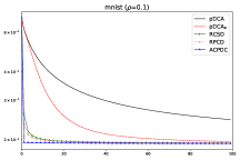
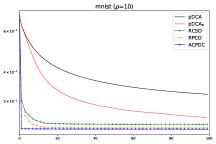
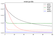
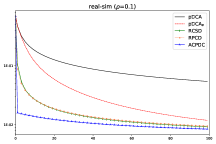
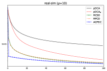
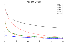
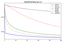
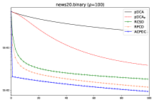
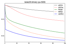
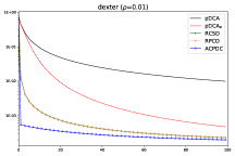
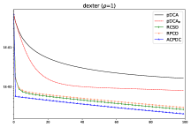
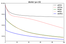
Figure 1: Experimental results on logistic loss classification with largest-$k$ norm penalty. $y$-axis: objective value (log scaled). $x$-axis: number of passes to the dataset. Test datasets (from top to bottom): mnist, resl-sim, news20.binary and dexter.

Smoothed $l_{1}$ loss + SCAD penalty

Our next experiment targets the $l_{1}$ loss regression with SCAD penalty:

$$\min_{x\in\mathbb{R}^{d}}F(x)=\frac{1}{n}{\textstyle{\sum}}_{i=1}^{n}\bigl{|}b_{i}-a_{i}^{T}x\bigr{|}+\frac{\rho}{d}\psi_{\lambda,\theta}(x).$$ (61)

Due to the nonsmooth, convex and inseparable part, Problem (61) does not exactly satisfy our assumption. Fortunately, by introducing a small term $\delta$, we can approximate $l_{1}$ loss by Huber loss $H_{\delta}(a)$:

$$H_{\delta}(a)=\begin{cases}\frac{a^{2}}{2\delta}&|a|\leq\delta\\ |a|-\tfrac{\delta}{2}&\text{o.w.}\end{cases},\quad\delta>0.$$

Our problem of interest, thus, follows:

$$\min_{x\in\mathbb{R}^{d}}F_{\delta}(x)=\frac{1}{n}\sum_{i=1}^{n}H_{\delta}(b_{i}-a_{i}^{T}x)+\frac{\rho}{d}\psi_{\lambda,\theta}(x),$$ (62)

Although smooth approximation introduces an $O(\delta)$ error, it allows us to minimize $F_{\delta}(x)$ fast by using the gradient information. It is easy to verify that $f_{\delta}(x)=\frac{1}{n}\sum_{i=1}^{n}H_{\delta}(b_{i}-a_{i}^{T}x)$ is block-wise Lipschitz smooth with $\frac{\|Ae_{i}\|^{2}}{n\delta}.$ In view of the Lipschitz smoothness of $f_{\delta}(x)$ and the weak convexity of $\psi_{\lambda,\theta}(x)$, $F_{\delta}(x)$ has a condition number of $O(\frac{\rho\,(\theta-1)}{d\,\delta})$. To set the parameters, we choose $\delta$ in the range $\{10^{-2},10^{-3}\}$. Clearly, $F_{\delta}$ is more difficult to minimize when $\delta$ is relatively small.

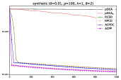
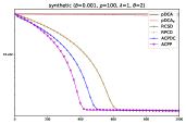
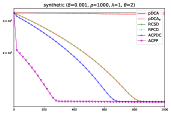
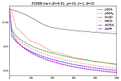
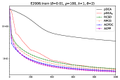
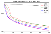
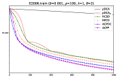
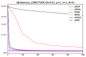
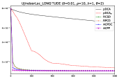
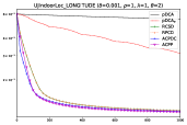
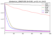
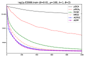
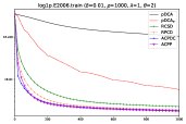
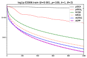
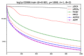
Figure 2: Experimental results on smoothed $l_{1}$ regression with SCAD penalty. $y$-axis: objective value (log scaled). $x$-axis: number of passes to the dataset. Test datasets (from top to bottom): synthetic, E2006-tfidf and UJIndoorLoc and E2006-log1p.

We conduct the experiments on datasets synthetic, E2006, UJIndoorLoc and log1p.E2006. In UJIndoorLoc, we consider predicting the location (longitude) of users inside of buildings. The dataset is preprocessed by rescaling and shifting the longitude values to $[-1,1]$. We compare all our proposed CD methods and the gradient methods pDCA and $\text{pDCA}_{e}$; convergence performance is shown in Figure 2. When the value of $\delta$ decreases, the approximation function $F_{\delta}$ is increasingly ill-conditioned, thereby being increasingly difficult to optimize. Indeed, we observe that the convergence of all the tested algorithms slows down when $\delta$ decreases from $10^{-2}$ to $10^{-3}$. Meanwhile, we observe that, CD methods still perform consistently better than gradient-based methods, and $\text{pDCA}_{e}$ performs consistently better than pDCA. Moreover, we find that both ACPDC and ACPP exhibit fast convergence and they both outperform RCSD and RPCD, further confirming the advantage of using ACD in the nonconvex settings.

8 Conclusion

In this paper, we developed novel CD methods for minimizing a class of nonsmooth and nonconvex functions. We developed randomized coordinate subgradient descent (RCSD) and randomly permuted coordinate descent (RPCD) methods, which naturally extend randomized coordinate descent and cyclic coordinate descent, respectively, to the nonsmooth and nonconvex settings, and establish their asymptotic convergence to critical points and novel complexity results. We also developed a new randomized proximal DC algorithm (ACPDC) for composite DC problems and a new randomized proximal point algorithm (ACPP) for weakly convex problems, based on the fast convergence of ACD for convex programming. We developed new optimality measures and established iteration complexities for the proposed algorithms. Both theoretical and experimental results demonstrate the advantage of our proposed CD approaches over state-of-the-art gradient-based methods.

Convergence of ACD for convex smooth optimization

In this section, we propose Algorithm 8, a variant of ACD method with non-uniform sampling, for unconstrained smooth optimization.

Theorem 16.

In Algorithm 8, choose the probability $p_{i}={L_{i}^{(1-s)/2}}/{T_{(1-s)/2}}$, $i\in[m]$. Define $\Gamma_{k}=\prod_{i=0}^{k}(1-\alpha_{i})^{-1}$, and assume that $\beta_{k}$, $\alpha_{k}$, $\gamma$ satisfy:

$$\mu_{s} \geq\gamma$$ (63)

$$\beta_{k} \geq\alpha_{k}T_{(1-s)/2}^{2},\quad k=0,1,2,...,$$ (64)

$$\Gamma_{k}\alpha_{k}(\beta_{k}+\gamma) \geq\Gamma_{k+1}\alpha_{k+1}\beta_{k+1}\quad k=0,1,2,....$$ (65)

Then we have

$$\Gamma_{K-1}\mathbb{E}[f(x^{K})-f(x^{*})]\leq f(x^{0})-f(x^{*})+\tfrac{\Gamma_{0}\alpha_{0}\beta_{0}}{2}\|x^{*}-x^{0}\|_{[s]}^{2}.$$

In particular, if we choose $\alpha_{k}=\tfrac{\sqrt{\mu_{s}}}{\sqrt{\mu_{s}}+T_{(1-s)/2}}$ and $\beta_{k}=\sqrt{\mu_{s}}T_{(1-s)/2}$ and $\gamma=\mu_{s}$, then we have

$$\mathbb{E}[f(x^{K})-f(x^{*})]\leq\left(1-\tfrac{\sqrt{\mu_{s}}}{\sqrt{\mu_{s}}+T_{(1-s)/2}}\right)^{K}\left[f(x^{0})-f(x^{*})+\tfrac{\mu_{s}}{2}\|x-x^{0}\|_{[s]}^{2}\right].$$

Proof.

We successively estimate the bound of $f(\bar{x}^{k+1})$ by

$$f(\bar{x}^{k+1}) \leq f(y^{k})+\left\langle\nabla f(y^{k}),\bar{x}^{k+1}-y^{k}\right\rangle+\tfrac{L_{i_{k}}}{2}\|\bar{x}^{k+1}-y^{k}\|^{2}$$

$$=(1-\alpha_{k})[f(y^{k})+\langle\nabla f(y^{k}),x^{k}-y^{k}\rangle]+\tfrac{L_{i_{k}}}{2}\|\bar{x}^{k+1}-y^{k}\|^{2}+\alpha_{k}f(y^{k})$$

$$\quad+\alpha_{k}\langle\nabla f(y^{k}),\tfrac{1}{p_{i_{k}}}\mathbf{U}_{i_{k}}z_{i_{k}}^{k+1}-y^{k}\rangle+\alpha_{k}\langle\nabla f(y^{k}),z^{k}-\tfrac{1}{p_{i_{k}}}\mathbf{U}_{i_{k}}z_{i_{k}}^{k}\rangle$$

$$\leq(1-\alpha_{k})f(x^{k})+\tfrac{L_{i_{k}}\alpha_{k}^{2}}{2p_{i_{k}}^{2}}\|z_{i_{k}}^{k}-z_{i_{k}}^{k+1}\|_{i_{k}}^{2}+\alpha_{k}f(x)-\tfrac{\alpha_{k}\mu_{s}}{2}\left\|x-y^{k}\right\|_{[s]}^{2}$$

$$\quad+\tfrac{\alpha_{k}}{p_{i_{k}}}\langle\nabla_{i_{k}}f(y^{k}),z_{i_{k}}^{k+1}-x_{i_{k}}\rangle+\alpha_{k}\langle\nabla f(y^{k}),\tfrac{1}{p_{i_{k}}}\mathbf{U}_{i_{k}}x_{i_{k}}-x\rangle$$

$$\quad+\alpha_{k}\langle\nabla f(y^{k}),z^{k}-\tfrac{1}{p_{i_{k}}}\mathbf{U}_{i_{k}}z_{i_{k}}^{k}\rangle,$$ (66)

where the first equality uses the following identity

$$\bar{x}^{k+1}=y^{k}+\tfrac{\alpha_{k}}{p_{i}}\mathbf{U}_{i_{k}}(z_{i_{k}}^{k+1}-z_{i_{k}}^{k})=(1-\alpha_{k})x^{k}+\tfrac{\alpha_{k}}{p_{i}}\mathbf{U}_{i_{k}}z_{i_{k}}^{k+1}+(\alpha_{k}z^{k}-\tfrac{\alpha_{k}}{p_{i}}\mathbf{U}_{i_{k}}z_{i_{k}}^{k}),$$

and the last inequality uses the strong convexity:

$$f(y^{k})+\left\langle\nabla f(y^{k}),x-y^{k}\right\rangle\leq f(x)-\tfrac{\mu_{s}}{2}\|x-y^{k}\|_{[s]}^{2}.$$

According to Lemma (2), we have

$$\tfrac{\alpha_{k}}{p_{i_{k}}}\left\langle\nabla_{i_{k}}f(y^{k}),z_{i_{k}}^{k+1}-x_{i_{k}}\right\rangle \leq\tfrac{\alpha_{k}\gamma}{2}[\|x-y^{k}\|_{[s]}^{2}-\|x-z^{k+1}\|_{[s]}^{2}-\|y^{k}-z^{k+1}\|_{[s]}^{2}]$$

$$\quad+\tfrac{\alpha_{k}\beta_{k}}{2}[\|x-z^{k}\|_{[s]}^{2}-\|x-z^{k+1}\|_{[s]}^{2}-\|z^{k}-z^{k+1}\|_{[s]}^{2}]$$

$$\leq\tfrac{\alpha_{k}\gamma}{2}\|x-y^{k}\|_{[s]}^{2}+\tfrac{\alpha_{k}\beta_{k}}{2}\|x-z^{k}\|_{[s]}^{2}$$

$$\quad-\tfrac{\alpha_{k}(\beta_{k}+\gamma)}{2}\|x-z^{k+1}\|_{[s]}^{2}-\tfrac{\alpha_{k}\beta_{k}}{2}\|z^{k}-z^{k+1}\|_{[s]}^{2}$$ (67)

In view of (64), we have

$$\tfrac{L_{i_{k}}\alpha_{k}^{2}}{2p_{i_{k}}^{2}}\|z_{i_{k}}^{k}-z_{i_{k}}^{k+1}\|_{i_{k}}^{2}-\tfrac{\alpha_{k}\beta_{k}}{2}\|z^{k}-z^{k+1}\|_{[s]}^{2}\leq\tfrac{\alpha_{k}^{2}T_{(1-s)/2}^{2}-\alpha_{k}\beta_{k}}{2}\|z^{k}-z^{k+1}\|_{[s]}^{2}\leq 0.$$

From (63), we have $\tfrac{\alpha_{k}\gamma}{2}[\|x-y^{k}\|_{[s]}^{2}\leq\tfrac{\alpha_{k}\mu_{s}}{2}\left\|x-y^{k}\right\|_{[s]}^{2}$.

Now putting (66) and (67) together, we obtain

$$f(\bar{x}^{k+1}) \leq(1-\alpha_{k})f(x^{k})+\alpha_{k}f(x)+\tfrac{\alpha_{k}\beta_{k}}{2}\|x-z^{k}\|_{[s]}^{2}-\tfrac{\alpha_{k}(\beta_{k}+\gamma)}{2}\|x-z^{k+1}\|_{[s]}^{2}$$

$$\quad+\alpha_{k}\langle\nabla f(y^{k}),\tfrac{1}{p_{i_{k}}}\mathbf{U}_{i_{k}}x_{i_{k}}-x\rangle+\alpha_{k}\langle\nabla f(y^{k}),z^{k}-\tfrac{1}{p_{i_{k}}}\mathbf{U}_{i_{k}}z_{i_{k}}^{k}\rangle.$$ (68)

We next take the expectation on both sides of (68) over $i_{k}$. Notice the identity $\mathbb{E}_{i_{k}}\langle\nabla f(y^{k}),\tfrac{1}{p_{i_{k}}}\mathbf{U}_{i_{k}}x_{i_{k}}-x\rangle=0$ and $\mathbb{E}_{i_{k}}\langle\nabla f(y^{k}),z^{k}-\tfrac{1}{p_{i_{k}}}\mathbf{U}_{i_{k}}z_{i_{k}}^{k}\rangle=0$. Moreover, notice that for option II of Algorithm 7, we have $f(x^{k+1})+\tfrac{1}{2L_{i_{k}}}\|\nabla_{i_{k}}f(\bar{x}^{k+1})\|_{i_{k}}^{2}\leq f(\bar{x}^{k+1})$, hence we always guarantee $f(x^{k+1})\leq f(\bar{x}^{k+1})$. Putting all these pieces together, we have

$$\mathbb{E}_{i_{k}}[f(x^{k+1})-f(x)]\leq(1-\alpha_{k})[f(x^{k})-f(x)]+\tfrac{\alpha_{k}\beta_{k}}{2}\|x-z^{k}\|_{[s]}^{2}-\tfrac{\alpha_{k}(\beta_{k}+\gamma)}{2}\mathbb{E}_{i_{k}}\|x-z^{k+1}\|_{[s]}^{2}.$$

Note that $\Gamma_{k}=\prod_{i=0}^{k}\tfrac{1}{1-\alpha_{i}}$. Then, multiplying both sides of the above relation by $\Gamma_{k}$, and then summing up over $k=0,1,2,...,K-1$, we have

$$\Gamma_{K-1}\mathbb{E}[f(x^{K})-f(x)] \leq f(x^{0})-f(x)+\tfrac{\Gamma_{0}\alpha_{0}\beta_{0}}{2}\|x-x^{0}\|_{[s]}^{2}$$

$$\quad-\tfrac{\Gamma_{K-1}\alpha_{K-1}(\beta_{K-1}+\gamma)}{2}\mathbb{E}\|x-z^{K}\|_{[s]}^{2}.$$

Moreover, if we choose $\alpha_{k}=\tfrac{\sqrt{\mu_{s}}}{\sqrt{\mu_{s}}+T_{(1-s)/2}}$, $\beta_{k}=\sqrt{\mu_{s}}T_{(1-s)/2}$ and $\gamma=\mu_{s}$, then we have

$$\mathbb{E}[f(x^{K})-f(x^{*})]\leq\left(1-\tfrac{\sqrt{\mu_{s}}}{\sqrt{\mu_{s}}+T_{(1-s)/2}}\right)^{K}\left[f(x^{0})-f(x^{*})+\tfrac{\mu_{s}}{2}\|x-x^{0}\|_{[s]}^{2}\right].$$

∎

The best rate of Algorithm 8 is achieved at $s=0$. We summarize the complexity of such a case in the following corollary.

Corollary 17.

Let $x^{*}$ be the optimal solution. Assume that $f(\cdot)$ is strongly convex with norm $\|\cdot\|^{2}$. If we choose $s=0$, then for any $\epsilon>0$,

$$N_{\epsilon}\in\mathcal{O}\left(\tfrac{\sqrt{\mu_{0}}+\sum_{i=1}^{m}\sqrt{L_{i}}}{\sqrt{\mu_{0}}}\log\tfrac{f(x^{0})-f(x^{*})+\tfrac{\mu_{0}}{2}\|x-x^{0}\|^{2}}{\epsilon}\right)$$

iterations of Algorithm 8 are required to obtain an expected $\epsilon$-accurate solution.

Proof.

From Theorem 13, we have that

$$\mathbb{E}[f(x^{K})-f(x^{*})] \leq\left(1-\tfrac{\sqrt{\mu_{0}}}{\sqrt{\mu_{0}}+T_{1/2}}\right)^{K}\left[f(x^{0})-f(x^{*})+\tfrac{\mu_{0}}{2}\|x-x^{0}\|^{2}\right]$$

$$\leq\exp\left(-\tfrac{\sqrt{\mu_{0}}}{\sqrt{\mu_{0}}+T_{1/2}}K\right)\left[f(x^{0})-f(x^{*})+\tfrac{\mu_{0}}{2}\|x-x^{0}\|^{2}\right].$$

∎

References

- [1] Z. Allen-Zhu, Z. Qu, P. Richtárik, and Y. Yuan, Even faster accelerated coordinate descent using non-uniform sampling, International Conference on MachineLearning, (2016), pp. 1110–1119.
- [2] N. T. An and N. M. Nam, Convergence analysis of a proximal point algorithm for minimizing differences of functions, Optimization, 66 (2017), pp. 129–147.
- [3] A. Beck and N. Hallak, Optimization problems involving group sparsity terms, MathematicalProgramming, (2018), pp. 1–29.
- [4] A. Beck and L. Tetruashvili, On the convergence of block coordinate descent type methods, SIAM J. onOptimization, 23 (2013), pp. 2037–2060.
- [5] Y. Carmon, J. C. Duchi, O. Hinder, and A. Sidford, Accelerated methods for non-convex optimization, arXiv preprintarXiv:1611.00756, (2016).
- [6] C.-C. Chang and C.-J. Lin, LIBSVM: A library for support vector machines, ACM Transactions on Intell. Systems Technology, 2 (2011), pp. 27:1–27:27. Software available at http://www.csie.ntu.edu.tw/~cjlin/libsvm.
- [7] C. D. Dang and G. Lan, Stochastic block mirror descent methods for nonsmooth and stochastic optimization, SIAM J. onOptimization, 25 (2015), pp. 856–881.
- [8] D. Davis and B. Grimmer, Proximally guided stochastic subgradient method for nonsmooth, nonconvex problems, SIAM J. onOptimization, 29 (2019), pp. 1908–1930.
- [9] D. Drusvyatskiy and C. Paquette, Efficiency of minimizing compositions of convex functions and smooth maps, MathematicalProgramming, (2018), pp. 1–56.
- [10] D. Dua and C. Graff, UCI machine learning repository, 2017.
- [11] J. C. Duchi and F. Ruan, Stochastic methods for composite and weakly convex optimization problems, SIAM J. onOptimization, 28 (2018), pp. 3229–3259.
- [12] J. Fan and R. Li, Variable selection via nonconcave penalized likelihood and its oracle properties, J. American StatisticalAssociation, 96 (2001), pp. 1348–1360.
- [13] S. Ghadimi and G. Lan, Stochastic first-and zeroth-order methods for nonconvex stochastic programming, SIAM J. onOptimization, 23 (2013), pp. 2341–2368.
- [14] , Accelerated gradient methods for nonconvex nonlinear and stochastic programming, MathematicalProgramming, 156 (2016), pp. 59–99.
- [15] P. Gong, C. Zhang, Z. Lu, J. Z. Huang, and J. Ye, A general iterative shrinkage and thresholding algorithm for non-convex regularized optimization problems, International Conference on MachineLearning, 28 (2013), pp. 37–45.
- [16] L. T. K. Hien, N. Gillis, and P. Patrinos, Inertial block mirror descent method for non-convex non-smooth optimization, arXiv preprintarXiv:1903.01818, (2019).
- [17] M. Hong, M. Razaviyayn, Z. Q. Luo, and J. S. Pang, A unified algorithmic framework for block-structured optimization involving big data: With applications in machine learning and signal processing, IEEE Signal ProcessingMagazine, 33 (2016), pp. 57–77.
- [18] K. Khamaru and M. J. Wainwright, Convergence guarantees for a class of non-convex and non-smooth optimization problems, International Conference on MachineLearning, (2018), pp. 2606–2615.
- [19] W. Kong, J. G. Melo, and R. D. Monteiro, Complexity of a quadratic penalty accelerated inexact proximal point method for solving linearly constrained nonconvex composite programs, arXiv preprintarXiv:1802.03504, (2018).
- [20] G. Lan and Y. Yang, Accelerated stochastic algorithms for nonconvex finite-sum and multi-block optimization, arXiv preprintarXiv:1805.05411, (2018).
- [21] Q. Lin, Z. Lu, and L. Xiao, An accelerated randomized proximal coordinate gradient method and its application to regularized empirical risk minimization, SIAM J. onOptimization, 25 (2015), pp. 2244–2273.
- [22] Y. Nesterov, Efficiency of coordinate descent methods on huge-scale optimization problems, SIAM J. onOptimization, 22 (2012), pp. 341–362.
- [23] Y. Nesterov and S. U. Stich, Efficiency of accelerated coordinate descent method on structured optimization problems, SIAM J. onOptimization, 27 (2017), pp. 110–123.
- [24] M. Nouiehed, J.-S. Pang, and M. Razaviyayn, On the pervasiveness of difference-convexity in optimization and statistics, MathematicalProgramming, (2018), pp. 1–28.
- [25] A. Patrascu and I. Necoara, Efficient random coordinate descent algorithms for large-scale structured nonconvex optimization, J. GlobalOptimization, 61 (2015), pp. 19–46.
- [26] P. Richtarik and M. Takac, Iteration complexity of randomized block-coordinate descent methods for minimizing a composite function, MathematicalProgramming, 144 (2014), pp. 1–38.
- [27] P. Richtarik and M. Takac, Parallel coordinate descent methods for big data optimization, MathematicalProgramming, 156 (2016), pp. 433–484.
- [28] H. A. L. Thi and T. P. Dinh, Dc programming and dca: thirty years of developments, MathematicalProgramming, 169 (2018), pp. 5–68.
- [29] H. L. Thi, T. P. Dinh, H. Le, and X. Vo, DC approximation approaches for sparse optimization, European J. OperationalResearch, 244 (2015), pp. 26–46.
- [30] B. Wen, X. Chen, and T. K. Pong, A proximal difference-of-convex algorithm with extrapolation, Computational Optimization Applications, 69 (2018), pp. 297–324.
- [31] Y. Xu, Q. Qi, Q. Lin, R. Jin, and T. Yang, Stochastic optimization for dc functions and non-smooth non-convex regularizers with non-asymptotic convergence, arXiv preprintarXiv:1811.11829, (2018).
- [32] Y. Xu and W. Yin, A globally convergent algorithm for nonconvex optimization based on block coordinate update, J. ScientificComputing, 72 (2017), pp. 700–734.
- [33] J. ya Gotoh, A. Takeda, and K. Tono, DC formulations and algorithms for sparse optimization problems, MathematicalProgramming, 169 (2018), pp. 141–176.
- [34] A. L. Yuille and A. Rangarajan, The concave-convex procedure (CCCP), in Advances in Neural Information Processing Systems 14, 2002, pp. 1033–1040.
- [35] C.-H. Zhang and T. Zhang, A general theory of concave regularization for high-dimensional sparse estimation problems, Statistical