Enforcing Analytic Constraints in Neural-Networks Emulating Physical Systems

Abstract

Neural networks can emulate nonlinear physical systems with high accuracy, yet they may produce physically-inconsistent results when violating fundamental constraints. Here, we introduce a systematic way of enforcing nonlinear analytic constraints in neural networks via constraints in the architecture or the loss function. Applied to convective processes for climate modeling, architectural constraints enforce conservation laws to within machine precision without degrading performance. Enforcing constraints also reduces errors in the subsets of the outputs most impacted by the constraints.
Main Repository: https://github.com/raspstephan/CBRAIN-CAM
Figures and Tables: https://github.com/tbeucler/CBRAIN-CAM/blob/master/notebooks/tbeucler_devlog/042_Figures_PRL_Submission.ipynb

I Introduction

Many fields of science and engineering (e.g., fluid dynamics, hydrology, solid mechanics, chemistry kinetics) have exact, often analytic, closed-form constraints, i.e. constraints that can be explicitly written using analytic functions of the system’s variables. Examples include translational or rotational invariance, conservation laws, or equations of state. While physically-consistent models should enforce constraints to within machine precision, data-driven algorithms often fail to satisfy well-known constraints that are not explicitly enforced. In particular, neural networks (NNs, [1]), powerful regression tools for nonlinear systems, may severely violate constraints on individual samples while optimizing overall performance.

Despite the need for physically-informed NNs for complex physical systems [2, 3, 4, 5], enforcing hard constraints [6] has been limited to physical systems governed by specific equations, such as advection equations [7, 8, 9], Reynolds-averaged Navier-Stokes equations [10, 11], boundary conditions of idealized flows [12], or quasi-geostrophic equations [13]. To address this gap, we introduce a systematic method to enforce analytic constraints arising in more general physical systems to within machine precision, namely the Architecture-Constrained NN or ACnet. We then compare ACnets to unconstrained (UCnets) and loss-constrained NNs (LCnets, in which soft constraints are added through a penalization term in the loss function [e.g., 14, 15, 16]) in the particular case of climate modeling, where the system is high-dimensional and the constraints (such as mass and energy conservation) are few but crucial [17].

II Theory

II.1 Formulating the Constraints

Consider a NN mapping an input vector $\bm{x}\in\mathbb{R}^{m}\$ to an output vector $\bm{y}\in\mathbb{R}^{p}\$. Enforcing constraints is easiest for linearly-constrained NNs, i.e. NNs for which the constraints $\left({\cal C}\right)\$can be written as a linear system of rank $n$:

$$\left({\cal C}\right)\overset{\mathrm{def}}{=}\left\{\bm{C}\left[\begin{array}[]{c}\bm{x}\\ \bm{y}\end{array}\right]=\bm{0}\right\}.$$ (1)

We call $\bm{C}\in\mathbb{R}^{n}\times\mathbb{R}^{m+p}\$the constraints matrix, and use bold font for vectors and tensors to distinguish them from scalars. For the regression problem to have non-unique solutions, the number of independent constraints $n$ has to be strictly less than $m+p$.

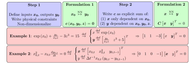
Figure 1: Framework to treat constrained regression problems using linearly-constrained NNs, with two examples: (1) A regression problem with one nonlinear constraint, and (2) a time-prediction problem with one differential nonlinear constraint that we discretize using a forward Euler method of timestep $\Delta t$. Note that the choice of $\bm{x},\bm{y}$, and $\bm{C}$ is not unique.

In Figure 1, we consider a generic regression problem subject to analytic constraints $\left({\cal C}\right)$ that may be nonlinear, and propose how to formulate a linearly-constrained NN. First, define the regression’s inputs $\bm{x_{0}}$ and outputs $\bm{y_{0}}$, which respectively become the temporary NN’s features and targets. Then (Formulation 1), write the constraints $\left({\cal C}\right)$ as an identically zero function $\bm{c}$ of the inputs, the outputs, and additional parameters $\bm{z}$ the constraints may involve. We recommend non-dimensionalizing all variables to facilitate the design, interpretation, and performance of the loss function. While the function $\bm{c}$ may be nonlinear, it can always be written as the sum of: (1) terms $\bm{x}$ that only depend on inputs and (2) terms $\bm{y}$ that depend on inputs, outputs and additional parameters. Thus the constraints can be written as:

$$\bm{c\left(x_{0},y_{0},z\right)}=\bm{C}\begin{bmatrix}\bm{x\left(x_{0}\right)}\\ \bm{y\left(x_{0},y_{0},z\right)}\end{bmatrix},$$ (2)

where $\bm{C}$ is a matrix. Finally (Formulation 2), choose $\bm{x}$ and $\bm{y}$ as the NN’s new inputs and outputs. If $\bm{x}$ and $\bm{y}$ are not bijective functions of $\bm{\left(x_{0},y_{0}\right)}$, add variables to the NN’s inputs and outputs to recover $\bm{x_{0}}$ and $\bm{y_{0}}$ after optimization (e.g., we add $x_{0,t}$ and $y_{0,t-1}$ to $\bm{x}$ in Example 2). We are now in a position to build a computationally-efficient NN that satisfies the linear constraints $\left({\cal C}\right)$.

II.2 Enforcing the Constraints

Consider a NN trained on preexisting measurements of $\bm{x}\$and $\bm{y}$. For simplicity’s sake, we measure the quality of its output $\bm{y_{\mathrm{NN}}}$ using a standard mean-squared error (MSE) misfit:

$$\mathrm{MSE}\left(\bm{y_{\mathrm{Truth}}},\bm{y_{\mathrm{NN}}}\right)\overset{\mathrm{def}}{=}\left\|\bm{y_{\mathrm{Err}}}\right\|_{2}\overset{\mathrm{def}}{=}\frac{1}{p}\sum_{k=1}^{p}y_{\mathrm{Err},k}^{2},$$ (3)

where we have introduced the error vector, defined as the difference between the NN’s output and the “truth”:

$$\bm{y_{\mathrm{Err}}}\overset{\mathrm{def}}{=}\bm{y_{\mathrm{NN}}}-\bm{y_{\mathrm{Truth}}}.$$ (4)

In the reference case of an “unconstrained network” (UCnet), we optimize a multi-layer perceptron [e.g., 18, 19] using $\mathrm{MSE}\$as its loss function $\cal{L}$. To enforce the constraints $\left({\cal C}\right)\$within NNs, we consider two options:

(1) Constraining the loss function (LCnet, soft constraints): We first test a soft penalization of the NN for violating physical constraints using a penalty ${\cal P}$, defined as the mean-squared residual from the constraints:

$${\cal P}\left(\bm{x},\bm{y_{\mathrm{NN}}}\right) \overset{\mathrm{def}}{=}\left\|\bm{C}\left[\begin{array}[]{c}\bm{x}\\ \bm{y_{\mathrm{NN}}}\end{array}\right]\right\|_{2},$$ (5)

$$=\frac{1}{n}\sum_{i=1}^{n}\left(\sum_{j=1}^{m}C_{ij}x_{j}+\sum_{k=1}^{p}C_{i\left(k+m\right)}y_{\mathrm{NN},k}\right)^{2},$$

and given a weight $\alpha\in\left[0,1\right]\$in the loss function ${\cal L}$:

$${\cal L}\left(\alpha\right)=\alpha{\cal P}\left(\bm{x},\bm{y_{\mathrm{NN}}}\right)+\left(1-\alpha\right)\mathrm{MSE}\left(\bm{y_{\mathrm{Truth}}},\bm{y_{\mathrm{NN}}}\right).$$ (6)

(2) Constraining the architecture (ACnet, hard constraints): Alternatively, we treat the constraints as hard and augment a standard, optimizable NN with $n\$fixed conservation layers that sequentially enforce the constraints $\left({\cal C}\right)\$to within machine precision (Figure 2), while keeping the $\mathrm{MSE}\$as the loss function:

$$\left(\mathrm{ACnet}\right)\Rightarrow\begin{Bmatrix}\min\mathrm{MSE}\ \ \mathrm{s.t.}\ \ \bm{C}\begin{bmatrix}\bm{x}&\bm{y_{\mathrm{NN}}}\end{bmatrix}^{T}=\bm{0}\end{Bmatrix}$$ (7)

The optimizable NN calculates a “direct” output whose size is $p-n$. We then calculate the remaining output’s components of size $n$ as exact “residuals” from the constraints. Concatenating the “direct” and “residual” vectors results in the full output $\bm{y_{\mathrm{NN}}}\$that satisfies the constraints to within machine precision. Since our loss uses the full output $\bm{y_{\mathrm{NN}}}$, the gradients of the loss function are passed through the constraints layers during optimization, meaning that the final NN’s weights and biases depend on the constraints $\left({\cal C}\right)$. ACnet improves upon the common approach of calculating “residual” outputs after training because ACnet exposes the NN to “residual” output data during training (SM C.3). A possible implementation of the constraints layer uses custom (Tensorflow in our case) layers with fixed parameters that solve the system of equations $\left({\cal C}\right)\$, in row-echelon form, from the bottom to the top row (SM B.1). Note that we are free to choose which outputs to calculate as “residuals”, which introduces $n$ new hyperparameters (SM B.2).

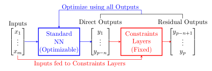
Figure 2: ACnet: Direct outputs are calculated using a standard NN, while the remaining outputs are calculated as residuals from the fixed constraints layers.

II.3 Linking Constraints to Performance

Intuitively, we might expect the NNs’ performance to improve once we enforce constraints arising in physical systems with few degrees of freedom, but this may not hold true with many degrees of freedom. We formalize the link between constraints and performance by: (1) decomposing the NN’s prediction into the “truth” and error vectors following equation 4; and (2) assuming that constraints exactly hold for the “truth” (no errors in measurement). This yields:

$$\bm{C}\left[\begin{array}[]{c}\bm{x}\\ \bm{y_{\mathrm{NN}}}\end{array}\right]\overset{\mathrm{def}}{=}\overbrace{\bm{C}\left[\begin{array}[]{c}\bm{x}\\ \bm{y_{\mathrm{Truth}}}\end{array}\right]}^{\bm{0}}+\bm{C}\left[\begin{array}[]{c}\bm{0}\\ \bm{y_{\mathrm{Err}}}\end{array}\right].$$ (8)

Equation 8 relates how much the constraints are violated to the error vector. More explicitly, if we measure performance using the MSE, we may square each component of Equation 8. The resulting equation links how much physical constraints are violated to the squared error for each constraint of index $i\in\llbracket 1,n\rrbracket$:

$$\underbrace{\left(\bm{C}\left[\begin{array}[]{c}x\\ y_{\mathrm{NN}}\end{array}\right]\right)_{i}^{2}}_{\mathrm{Physical\ constraints}} =\underbrace{\sum_{k=1}^{p}C_{i\left(k+m\right)}^{2}y_{\mathrm{Err},k}^{2}}_{\mathrm{Squared-error}>0}$$ (9)

$$+\underbrace{\sum_{k=1}^{p}\sum_{l\neq k}C_{i\left(k+m\right)}C_{i\left(l+m\right)}y_{\mathrm{Err},k}y_{\mathrm{Err},l}}_{\mathrm{Cross-term}}$$

In ACnets, we strictly enforce physical constraints, setting the left-hand side of Equation 9 to 0, within numerical errors. As the squared error is positive-definite, the cross-term is always negative in ACnets as both terms sum up to 0. It is difficult to predict the cross-term before optimization, hence Equation 9 does not provide a-priori predictions of performance, even for ACnets. Instead, it links how much the NN violates constraints to how well it predicts outputs that appear in the constraints equations: the more negative the cross-term, the larger the squared error for a given violation of physical constraints.

III Application

III.1 Convective Parameterization for Climate Modeling

The representation of subgrid-scale processes in coarse-scale, numerical models of the atmosphere, referred to as subgrid parameterization, is a large source of error and uncertainty in numerical weather and climate prediction [e.g., 20, 21]. Machine-learning algorithms trained on fine-scale, process-resolving models can improve subgrid parameterizations by faithfully emulating the effect of fine-scale processes on coarse-scale dynamics [e.g., 22, 23, 24, 25, see Section 2 of Rasp [26] for a detailed review]. The problem is that none of these parameterizations exactly follow conservation laws (e.g., conservation of mass, energy). This is critical for long-term climate projections, as the spurious energy production may both exceed the projected radiative forcing from greenhouse gases and result in large thermodynamic drifts or biases over a long time-period. Motivated by this shortcoming, we build a NN parameterization of convection and clouds that we constrain to conserve 4 quantities: column-integrated energy, mass, longwave radiation, and shortwave radiation.

III.2 Model and Data

We use the Super-Parameterized Community Atmosphere Model 3.0 [27] to simulate the climate for two years in aquaplanet configuration [28], where the surface temperatures are fixed with a realistic equator-to-pole gradient [29]. Following [24]’s sensitivity tests, we use 42M samples from the simulation’s first year to train the NN (training set) and 42M samples from the simulation’s second year to validate the NN (validation set). Since we use the validation set to adjust the NN’s hyperparameters and avoid overfitting, we additionally introduce a test set using 42M different samples from the simulation’s second year to provide an unbiased estimator of the NNs’ performances. Note that each sample represents a single atmospheric column at a given time, longitude, and latitude.

III.3 Formulating the Conservation Laws in a Neural Network

The parameterization’s goal is to predict the rate at which sub-grid convection vertically redistributes heat and water based on the current large-scale thermodynamic state. We group all variables describing the local climate in an input vector $\bm{x}$ of size 304 (5 vertical profiles with 30 levels each, prescribed large-scale conditions $\bm{\mathrm{LS}}$ for all profiles of size 150, and 4 scalars):

$$\bm{x}=\left[\begin{array}[]{ccc}\left(\bm{q_{v}},\bm{q_{l}},\bm{q_{i}},\bm{T},\bm{v},\bm{\mathrm{LS}},p_{s},S_{0}\right)&\mathrm{SHF}&\mathrm{LHF}\end{array}\right]^{T},$$ (10)

where all variables are defined in SM A. We then concatenate the time-tendencies from convection and the additional variables involved in the conservation laws to form an output vector $\bm{y}\$of size 216 (7 vertical profiles with 30 levels, followed by 6 scalars):

$$\bm{y}=\left[\begin{array}[]{ccccccccccccc}\bm{\dot{q}_{v}}&\bm{\dot{q}_{l}}&\bm{\dot{q}_{i}}&\bm{\dot{T}}&\bm{\dot{T}_{KE}}&\bm{\mathrm{lw}}&\bm{\mathrm{sw}}&\mathrm{LW_{t}}&\mathrm{LW_{s}}&\mathrm{SW_{t}}&\mathrm{SW_{s}}&P&P_{i}\end{array}\right]^{T},$$ (11)

We normalize all variables to the same units before non-dimensionalizing them using the constant $1\textnormal{W\ m}^{-2}$ (SM A.5). Finally, we derive the dimensionless conservation laws (SM A.1-A.4) and write them as a sparse matrix of size $4\times\left(304+218\right)\$:

$$\bm{C}=\left[\begin{array}[]{cccccccccccccccc}\bm{0}&1&\ell_{s}&-\ell_{s}\bm{\delta p}&-\ell_{f}\bm{\delta p}&\bm{0}&-\bm{\delta p}&\bm{\delta p}&\bm{0}&\bm{0}&-1&1&1&-1&-\ell_{f}&\ell_{f}\\ \bm{0}&0&1&-\bm{\delta p}&-\bm{\delta p}&-\bm{\delta p}&\bm{0}&\bm{0}&\bm{0}&\bm{0}&0&0&0&0&-1&0\\ \bm{0}&0&0&\bm{0}&\bm{0}&\bm{0}&\bm{0}&\bm{0}&\bm{\delta p}&\bm{0}&1&-1&0&0&0&0\\ \bm{0}&0&0&\bm{0}&\bm{0}&\bm{0}&\bm{0}&\bm{0}&\bm{0}&\bm{\delta p}&0&0&-1&1&0&0\end{array}\right],$$ (12)

that acts on $\bm{x}\$and $\bm{y}\$to yield Equation 1.

Each row of the constraints matrix $\bm{C}\$describes a different conservation law: The first row is column-integrated enthalpy conservation (here equivalent to energy conservation), the second row is column-integrated water conservation (here equivalent to mass conservation), the third row is column-integrated longwave radiation conservation and the last row is column-integrated shortwave radiation conservation.

III.4 Implementation

We implement the three NN types and a multi-linear regression baseline using the Tensorflow library [30] version 1.13 with Keras [31] version 2.2.4: (1) LCnets for which we vary the weight $\alpha$ given to conservation laws from 0 to 1 (Equation 6), (2) our reference ACnet, and (3) UCnet, i.e. an unconstrained LCnet of weight $\alpha=0$. In our reference ACnet, we write the constraints layers in Tensorflow to solve the system of equations $\left({\cal C}\right)$ from bottom to top, and calculate surface tendencies as residuals of the conservation equations (SM B.1); switching the “residual” outputs to different vertical levels does not significantly change the validation loss nor the constraints penalty (SM B.3). After testing multiple architectures and activation functions (SM C.2), we chose 5 hidden layers of 512 nodes with leaky rectified linear-unit activations as our standard multi-layer perceptron architecture, resulting in $\sim$1.3M trainable parameters. We optimized the NN’s weights and biases with the RMSprop optimizer [32] for LCnets (because it was more stable than the Adam optimizer [33]), used Sherpa for hyperparameter optimizations [34], and saved the NN’s state of minimal validation loss over 20 epochs.

III.5 Results

In Figure 3a, we compare mean performance (measured by MSE) and by how much physical constraints are violated (measured by $\cal{P}$) for the three NN types. As expected, we note a monotonic trade-off between performance and constraints as we increase $\alpha$ from 0 to 1 in the loss function. This trade-off is well-measured by MSE and $\cal P$ across the training, validation, and test sets (SM Table V). Interestingly, the physical constraints are easier to satisfy than reducing MSE in our case, likely because it is difficult to deterministically predict precipitation, which is strongly non-Gaussian, inherently stochastic, and whose error contributes to a large portion of MSE. Despite this, UCnet may violate physical constraints more than our multi-linear regression baseline.

Our first key result is that ACnet performs nearly as well as our lowest-MSE UCnet on average (to within 3$\%$) while satisfying constraints to $\sim\left(10^{-9}\%\right)$ (SM C.1). This result holds across the training, validation and test sets (SM Table IV). In our case, ACnets perform slightly less well than UCnet because they are harder to optimize and the “residual” outputs exhibit systematically larger errors (SM B.2). This systematic, unphysical bias can be remedied by multiplying the weights of these “residual” outputs in the loss function (SM B.3) by a factor $\beta>1$ (SM Equation 12 and SM Figure 2). $\beta$ can be objectively chosen alongside the “residual” outputs via formal hyperparameter optimization (SM C.2).

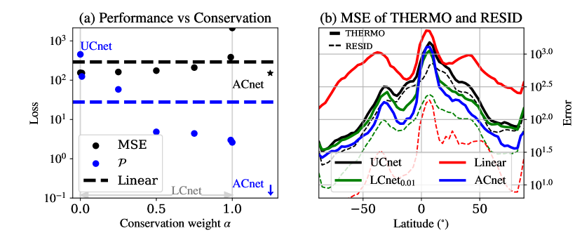
Figure 3: (a) MSE and $\cal{P}$ averaged over all samples of the test dataset for UCnet, LCnets of varying $\alpha$, and ACnet. The dashed lines indicate MSE and $\cal{P}$ for our multi-linear regression baseline. (b) Mean-squared error in the thermodynamic term (THERMO) and the enthalpy residual (RESID) versus latitude for our lowest-MSE NN in each category.

In Figure 3b, we compare how much the NNs violate column energy conservation (RESID) to the prediction of a variable that appears in that constraint: the total thermodynamic tendency in the enthalpy conservation equation (THERMO):

$$\overbrace{\left(\bm{C}\left[\begin{array}[]{c}x\\ y_{\mathrm{NN}}\end{array}\right]\right)_{1}}^{\mathrm{RESID}}=\overbrace{\bm{\delta p}\cdot\bm{\left(\dot{T}_{\mathrm{KE}}-\dot{T}-\ell_{s}\dot{q}_{v}-\ell_{f}\dot{q}_{l}\right)}}^{\mathrm{THERMO}}+...,$$ (13)

where the ellipsis includes the surface fluxes, radiation, and precipitation terms. ACnet predicts THERMO more accurately than all NNs (full blue line) by an amount closely related to how much each NN violates enthalpy consevation (dashed lines), followed by LCnet (full green line). This yields our second key result: Enforcing constraints, whether in the architecture or the loss function, can systematically reduce the error of variables that appear in the constraints. This result holds true across the training, validation, and test sets (SM Figure 4). However, possibly since our case has many degrees of freedom, it does not hold true for individual components of THERMO as their cross-term in Equation 9 is more negative for ACnet, nor does it hold for variables that are hard to predict deterministically (e.g., precipitation). Additionally, obeying conservation laws does not guarantee the ability to generalize well far outside of the training set, e.g. in the Tropics of a warmer climate (see Figure 3 of [35]). These results nuance the finding that physically constraining NNs systematically improves their generalization ability, which has been documented for machine learning emulation of low-dimensional idealized flows [12, 5], and motivate physically-constraining machine-learning algorithms capable of stochastic predictions [36] that are consistent across climates [35].

Finally, although the mapping presented in Section III has linear constraints, ACnets can also be applied to nonlinearly constrained mappings by using the framework presented in Figure 1. We give a concrete example in SM D, where we introduce the concept of “conversion layers” that transform nonlinearly constrained mappings into linearly-constrained mappings within NNs and without overly degrading performance (SM Table IX). Additionally, ACnets can be extended to incorporate inequality constraints on their “direct” outputs (by using positive-definite activation functions, discussed in SM E), making ACnets applicable to a broad range of constrained optimization problems.