Discovering mean residence time and escape probability from data of stochastic dynamical systems

Abstract

We present a method to learn mean residence time and escape probability from data modeled by stochastic differential equations. This method is a combination of machine learning from data (to extract stochastic differential equations as models) and stochastic dynamics (to quantify dynamical behaviors with deterministic tools). The goal is to learn and understand stochastic dynamics based on data. This method is applicable to sample path data collected from complex systems, as long as these systems can be modeled as stochastic differential equations.

Stochastic dynamical systems are appropriate models for randomly influenced systems. Understanding the complex dynamical behaviors of these systems is a challenge in diverse areas of science and engineering. In deterministic dynamical systems, invariant manifolds and other invariant structures provide global information for dynamical evolution. For stochastic dynamical systems, better quantitative analysis and understanding is needed because of limitations in our current analytical skills or computation capability. Fortunately, researchers are increasingly using data-driven methods for system identification and the discovery of dynamics. In this work, we propose a new approach to determine some computable dynamical quantities from data, such as the mean residence time and escape probability, which offer insights into global dynamics under uncertainty. We demonstrate the algorithm to be effective and robust, by reproducing known dynamics and evaluating errors for several prototypical stochastic dynamical systems with Brownian motions.

I Introduction

Stochastic dynamical systems arise in modeling molecular dynamics, mechanical and electrical engineering, climate dynamics, geophysical and environmental systems, among others. Advances in machine learning and data science are leading to new progresses in the analysis and understanding of complex dynamics for systems with massive observation data sets. Despite the rapid development of tools to extract governing equations from data, there has been slow progress in distilling quantities that may be used to explore stochastic dynamics. It is desirable to extract deterministic quantities that carry dynamical information of stochastic differential equations (SDEs). These deterministic quantities include moments for solution paths, probability density functions for solution paths, mean residence time and escape probability Duan02 ; Duan03 . These concepts help us to understand various phenomena in complex systems under uncertainty Arnold98 .

In this present paper, we will present a new approach to extract the underlying deterministic quantities, mean residence time and escape probability, that describe certain aspects of stochastic dynamics. In fact, mean residence time for a stochastic dynamical system quantifies how long the system stays in a region, and escape probability describes the likelihood of a system transition from one regime to another. Fortunately, these deterministic quantities can be determined by solving an elliptic partial differential equation as in Duan Duan03 , once the underlying stochastic differential equation model for the system evolution is discovered from data.

We assume that a data set is composed of sample paths governed by a stochastic differential equation (SDE) in $\mathbb{R}^{n}$,

$$dX_{t}=b(X_{t})dt+\sigma(X_{t})dB_{t},$$ (1.1)

where $b$ is an n-dimensional vector function, $\sigma$ is an $n\times m$ matrix function, and $B_{t}$ is an m-dimensional Brownian motion. This is the customary, probabilistic way of writing the equation

$$\frac{dX_{t}}{dt}=b(X_{t})+\sigma(X_{t})\frac{dB_{t}}{dt}.$$

Often, $b$ is called ‘drift’ and $\sigma$ is called ‘diffusion’. Assume that $b$ and $\sigma$ satisfy an appropriate local Lipschitz condition as follows:

$$\|b(x)-b(y)\|+\|\sigma(x)-\sigma(y)\|\leq K_{N}\|x-y\|,$$

for $\|x\|\leq N$, $\|y\|\leq N$ and $N>0$. Here the Lipschitz constant $K_{N}$ depends on the positive number $N$. The generator for this SDE system is a linear second-order differential operator:

$$Ag=b\cdot(\bigtriangledown g)+\frac{1}{2}\mathrm{Tr}[\sigma\sigma^{T}H(g)],~{}~{}~{}~{}g\in\mathbf{H}^{2}_{0}(\mathbb{R}^{n}),$$ (1.2)

where $H$ denotes the Hessian matrix of a multivariate function and $\mathrm{Tr}$ denotes the trace of a matrix. We view $A$ as a linear differential operator in Hilbert space $\mathbf{L}^{2}(\mathbb{R}^{n})$ with domain of definition $D(A)=\mathbf{H}^{2}_{0}(\mathbb{R}^{n})$. Furthermore, we assume that the generator $A$ is uniformly elliptic. That is for $x\in D$ and all $\xi\in\mathbb{R}^{n}$, there exists a positive constant $C$ such that

$$\sum^{n}_{i,j=1}(\sigma(x)\sigma^{T}(x))_{i,j}\xi_{i}\xi_{j}\geq C|\xi|^{2}.$$ (1.3)

We discuss mean residence time and escape probability as deterministic quantities that carry dynamical information for solution orbits of (1.1). For a bounded domain $D\subset\mathbb{R}^{n}$ (with boundary $\partial D$), the first exit time for a solution orbit starting at $x\in D$ is a stopping time defined as

$$\tau_{D}(\omega)\triangleq\inf\{t>0:X_{0}=x,X_{t}\in\partial D\}.$$

The mean residence time is defined as $u(x)\triangleq\mathbb{E}\tau_{D}(\omega)$. It is the mean residence time of a particle initially at $x$ inside $D$ until the particle first hits the boundary $\partial D$ or escapes from $D$. It turns out that the mean residence time $u$ of stochastic system (1.1) can be determined by solving a deterministic partial differential equation as follows:

$$Au = -1,$$ (1.4)

$$u|_{\partial D} = 0,$$ (1.5)

where $A$ is the generator defined as (1.2). To prove the existence and uniqueness of $u$, we recall the Dynkin’s formula (Theorem 7.4.1 in OksendalOksendal ):

$$\mathbf{E}^{x}[f(X_{\tau_{D}})]=f(x)+\mathbf{E}^{x}[\int_{0}^{\tau_{D}}Af(X_{s})ds],$$

for $f$ in the domain of definition of the generator $A$, $\mathbf{E}^{x}$ is the expectation with respect to the probability law $Q^{x}$ induced by a solution process $X_{t}$ starting at $x\in\mathbb{R}^{n}$. We take the continuous, bounded boundary value $\phi=0$ and the continuous inhomogeneous term $g=1$. By Theorem 9.3.3 in OksendalOksendal , which is a consequence of Dynkin’s formula, we know that the linear expectation $\mathbf{E}^{x}[\phi(X_{\tau_{D}})]+\mathbf{E}^{x}[\int_{0}^{\tau_{D}}g(X_{s})ds]$, which is just $\mathbf{E}_{\tau_{D}}=u(x)$, solves $Au=-1$ with the boundary condition $u|_{\partial D}=0$. Thus we can numerically compute mean residence time $u$ by solving elliptic partial differential equations, so we know how long the stochastic system (1.1) stays in the region $D$. For more details, see DuanDuan03 .

The escape probability is the likelihood that an orbit starting inside a domain $D$, exits from this domain first through a specific part $\Gamma$ of the boundary $\partial D$. Let $\Gamma$ be a subset of the boundary $\partial D$. We define the escape probability $p(x)$ from $D$ through $\Gamma$ as the likelihood that $X_{t}$ starting at $x$ exits from $D$ first through $p(x)=\mathbb{P}\{X_{\tau_{\partial D}}\in\Gamma\}$. We will show that the escape probability $p(x)$ solves a linear elliptic partial differential equation, with a specifically chosen Dirichlet condition as follow:

$$Ap = 0,$$ (1.6)

$$p|_{\Gamma} = 1,$$ (1.7)

$$p|_{\partial D\setminus\Gamma} = 0,$$ (1.8)

where $A$ is the generator defined as (1.2). Taking

$$\phi(x)=\left\{\begin{aligned} 1,&&{x\in\Gamma,}\\ 0,&&{x\in\partial D\setminus\Gamma,}\end{aligned}\right.$$

we have

$$\mathbf{E}[\phi(X_{\tau_{\partial D}}(x))] = \int_{\{\omega:X_{\tau_{\partial D}}(x)\in\Gamma\}}\phi(X_{\tau_{\partial D}}(x))d\mathbb{P}(\omega)$$

$$+\int_{\{\omega:X_{\tau_{\partial D}}(x)\in\partial D\setminus\Gamma\}}\phi(X_{\tau_{\partial D}}(x))d\mathbb{P}(\omega)$$

$$= \mathbb{P}\{\omega:X_{\tau_{\partial D}}(x)\in\Gamma\}$$

$$= p(x).$$

This means that $\mathbf{E}[\phi(X_{\tau_{\partial D}}(x))]$ is the escape probability $p(x)$ that we are looking for. We know $Ap=0$ together with $p|_{\Gamma}=1$ and $p|_{\partial D\setminus\Gamma}=0$ by Theorem 9.2.14 in OkendalOksendal . For more details, see DuanDuan03 . Moreover we suppose that solution orbits, i.e., ‘particles’ are initially uniformly distributed in $D$, then the average escape probability $P$ that a trajectory will leave $D$ through $\Gamma$ is $P=\frac{1}{D}\int_{D}p(x)dx$.

To obtain the mean residence time $u$ and escape probability $p$ from sample path data $X_{True}$ (with the underlying model (1.1)), we propose the following machine learning algorithm: First we collect sample path data $X_{True}$ by sample-wisely simulating (1.1) via Euler method (and treat these data as our observation data), then we try to learn the stochastic dynamical system model from these data with the following model ansatz

$$\dot{X}=\Theta\cdot\Xi,$$ (1.9)

where the basis $\Theta$ consists of polynomial functions $\{1,x,y,\cdots,x^{N}y^{N}\}$ together with the (generalized) time derivative of Brownian motion $dB_{t}/dt$, and $\Xi$ is the coefficient (or coordinate, or weight) under this basis. Here $\cdot$ denotes scalar product. Each column $\xi^{k}=[\xi_{1}^{k},\xi_{2}^{k},\cdots,\xi_{N}^{k}]$ of $\Xi$ is a vector of coefficients, determining which terms are active in the right-hand side for one of the row equations in (1.1). Brunton et al. Kutz considered such a learned model, with a basis not containing noise (i.e., $dB_{t}/dt$).

Furthermore, we set up a regression problem to determine coefficient $\Xi=[\xi^{1},\cdots,\xi^{n}]$ by minimizing the mean-square discrepancy (other metrics are possible) between the data $X_{True}$ (many samples), and the solution $X_{Learn}$ (many samples) for the learned (i.e., extracted) governing model (1.9). This will provide us the learned drift $b$ and learned diffusion $\sigma$, and thus we also have the extracted stochastic model (1.9), together with the learned generator $A$.

Finally, with this learned generator $A$, we compute mean residence time $u$ and escape probability $p$, by solving the deterministic partial differential equations (1.4)-(1.5) and (1.6)-(1.8), respectively. We verify that our algorithm is effective by estimating the error of the maximal mean residence time

$$\mbox{error}(u)=\max_{D}\|u_{Learn}-u_{True}\|,$$

and the error of the average escape probability

$$\mbox{error}(P)=\|P_{Learn}-P_{True}\|,$$

between the learned system (1.9) and the original system (1.1).

This paper is organized as follows. In section 2, we apply our method to learn a two-dimensional quasigeostrophic meandering jet model with additive noise and multiplicative noise, and compute the mean residence time and escape probability. In section 3, we illustrate our method to learn two three-dimensional systems (a linear damped oscillator and the well-known Lorenz system). We summarize and conclude in section 4 .

II Learning two dimensional stochastic dynamical systems

Zonal shear flows occur naturally in both oceans and the atmosphere. The Gulf stream is a well known example. Based on RAFOS floats observations of the Gulf Steam, Bower et al. Bower01 ; Bower02 viewed the fluid motion as a steady and eastward meander propagation in the moving frame, and divided the velocity field into three regimes: a central jet, exterior retrograde motion, and intermediate closed circulations above meander troughs and below crests. There was no exchange occurring between the three regimes in this model. Fluid particles in the intermediate regime execute periodic motion but never escape. However, float observations reveal that several particle trajectories pass through meander crests and troughs and then leave jet, which indicate that exchange does occur across some part of the Gulf Stream. Samelson Samelson01 modified the basic model and considered three different types of variability: a time-dependent spatially uniform meridional velocity superimposed on the basic flow, a time-dependent meander amplitude, and a propagating plane wave superimposed on the basic flow. In particular, he only considered time-periodic variabilities. Subsequently, SamelsonSamelson02 , del-Castillo-Negrete et al.Del , Pratt et al.Pratt01 , Beigie et al.Wiggins , Duan et al.Duan01 and Brannan et al.Duan02 have obtained a series of outcomes from the point of view of dynamical systems.

II.1 Discovering a kinematical model for a two-dimensional meandering jet

As an approximate solution to the quasigeostrophic model for two-dimensional geophysical flows Ped , the basic Bickley jet Del is

$$\psi(x,y)=-\tanh(y)+asech^{2}(y)\cos(kx)+cy,$$

where $a=0.01$, $c=\frac{1}{3}(1+\sqrt{1-\frac{3}{2}\beta})$, $k=\sqrt{6c}$, $0\leq\beta\leq\frac{2}{3}$. In this paper, we take $\beta=\frac{1}{3}$. Note $\beta=\frac{2\Omega}{r}\cos\theta$ is the meridional derivative of the Coriolis parameter, where $\Omega$ is the rotation rate of the earth and $r$ is the earth’s radius and $\theta$ is the latitude. This stream function $\psi(x,y)$ defines the basic meandering jet system $\dot{x}=-\psi_{y},\;\;\dot{y}=\psi_{x}$. The phase portrait for this deterministic system is in FIG. 1 (left). As it shows no fluid exchange between the eddies and the jet, it is not an appropriate model for a meandering jet.

Thus we incorporate random wind forcing and other fluctuations, either additive or multiplicative, in the model for the meandering jet and consequently, we consider the following two stochastic dynamical systems

$$dx = -\psi_{y}dt+\sigma dB_{1},$$ (2.1)

$$dy = \psi_{x}dt+\sigma dB_{2},$$ (2.2)

and

$$dx = -\psi_{y}dt+\sigma xdB_{1},$$ (2.3)

$$dy = \psi_{x}dt+\sigma ydB_{2},$$ (2.4)

where the noise intensity $\sigma$ satisfies $0<\sigma<1$, and $B_{1}(t)$, $B_{2}(t)$ are two independent Brownian motions. For both stochastic systems, a number of sample solution orbits are shown in FIG. 1 (middle, right). The central jet and two rows of recirculation eddies, which are called the northern and southern recirculation regions, are still visible. Outside the recirculation regimes are the exterior retrograde regimes. There is no exchange between regimes in unperturbed model, but exchange does occur in other two models with additive or multiplicative noises. These two stochastic models are more appropriate for modeling a meandering jet (as a simplified model for the Gulf Stream), as observations indicate fluid exchange.

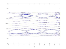
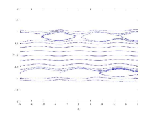
Figure 1: Lagrangian fluid trajectories of the original meandering jet system (2.1)-(2.4) with 20 initial positions: The fluid motion in the deterministic basic model ($\sigma=0$) (left) is steady, with no exchange of fluid between the eddies and the jet stream. Under additive noise ($\sigma=\sqrt{0.3}$) (middle) and multiplicative noise ($\sigma=\sqrt{0.3}$) (right), there are fluid exchanges between eddies and the jet stream.

A wide range of dynamical systems with intrinsic noise may be modeled with stochastic differential equations. However, identifying an appropriate SDE model from intermittent observations of the system is challenging, particularly if the dynamical process is nonlinear and the observations are noisy and indirect GaoDuan . Brunton et al. Kutz , Zhang et al. Lin , and Dunker et al. Bohner presented some approaches to discover or learn governing physical laws from data, with underlying differential equations models.

We use our machine learning algorithm to data, from system (2.1)-(2.2) or system (2.3)- (2.4), to learn their governing laws in terms of the following model

$$\dot{x} = \Theta\xi^{1},$$ (2.5)

$$\dot{y} = \Theta\xi^{2},$$ (2.6)

where $\Theta$ is a set of basis functions and $\Xi=[\xi^{1},\xi^{2}]$ defines the coefficients (or weights). To achieve this, the idea is as follows: First we collect a time series of the system state $(x(t_{i}),y(t_{i})),i=1,\cdots,20000,$ from system (2.1)-(2.2) or system (2.3)- (2.4) with noise intensity $\sigma=\sqrt{0.3}$, numerically by the Euler method (as our observation data $(x^{i}_{True},y^{i}_{True})$). Then we construct a library $\Theta$ consisting of basis functions with polynomials $\{1,x,y,\cdots,y^{5}\}$ and time derivative of Brownian motions $\{dB_{1}/dt,dB_{2}/dt\}$. We determine each column of coefficients $\xi^{k}=[\xi_{1}^{k},\xi_{2}^{k},\dots,\xi_{23}^{k}],k=1,2,$ by minimizing discrepancies $\mathbf{E}\sum_{i=1}^{20000}\|x^{i}_{True}-x^{i}_{Learn}\|^{2}$ and $\mathbf{E}\sum_{i=1}^{20000}\|y^{i}_{True}-y^{i}_{Learn}\|^{2}$. Here $(x^{i}_{Learn},y^{i}_{Learn})$ is the numerical solution of the learned meandering jet model (2.5)- (2.6) by Euler method. See Table 1 and Table 2.

Table 1: Identified coefficients for the learned meandering jet system (2.5)-(2.6). Data is numerically generated via Euler method for (2.1)-(2.2) (additive noise) with initial position $(-0.2,0.8)^{T}$ in the eddy, for time $t\in[0,200]$ with stepsize $0.01$.

basis	$\dot{x}$	$\dot{y}$
$1$	2.2114650e+00	1.1356876e+00
$x$	9.1670929e-01	-3.1053406e-01
$y$	-8.5337156e+00	-7.8830089e+00
$x^{2}$	2.1581933e-01	-5.8882267e-02
$xy$	-3.5406793e+00	1.2086885e+00
$y^{2}$	1.4806990e+01	2.1509332e+01
$x^{3}$	2.3163030e-02	-2.0687376e-03
$x^{2}y$	-6.4404598e-01	1.6556400e-02
$xy^{2}$	5.2163263e+00	-2.3046831e+00
$y^{3}$	-1.3568792e+01	-2.9159973e+01
$x^{4}$	6.6869672e-04	1.1181427e-02
$x^{3}y$	-7.3808685e-02	6.4410700e-02
$x^{2}y^{2}$	5.2977754e-01	2.2568117e-01
$xy^{3}$	-3.5783954e+00	2.2945214e+00
$y^{4}$	5.6314933e+00	1.9776092e+01
$x^{5}$	2.8510400e-04	1.2382566e-03
$x^{4}y$	-8.1958722e-04	-8.0288516e-04
$x^{3}y^{2}$	4.2275033e-02	-3.6886874e-02
$x^{2}y^{3}$	-1.1615968e-01	-1.7364994e-01
$xy^{4}$	9.9449264e-01	-9.0959557e-01
$y^{5}$	-6.8100788e-01	-5.3876952e+00
$dB1/dt$	5.4773030e-01	-9.7392788e-06
$dB2/dt$	2.7076551e-07	5.4771837e-01

Table 2: Identified coefficients for the learned meandering jet system (2.5)-(2.6). Data is numerically generated via Euler method for (2.3)-(2.4) (multiplicative noise) with initial position $(-0.2,0.8)^{T}$ in the eddy, for time $t\in[0,200]$ with stepsize $0.01$.

basis	$\dot{x}$	$\dot{y}$
$1$	4.6791584e+00	-7.5867935e+00
$x$	6.3006784e-01	-2.1087326e+00
$y$	-2.5483586e+01	4.3335141e+01
$x^{2}$	2.6109263e-01	-1.5952411e-01
$xy$	-1.7420741e+00	1.0564395e+01
$y^{2}$	6.1169058e+01	-9.4722221e+01
$x^{3}$	-3.1824190e-03	-1.0056540e-01
$x^{2}y$	-9.6615354e-01	-2.4673718e-01
$xy^{2}$	8.8535465e-01	-2.1532391e+01
$y^{3}$	-7.6829624e+01	9.6863629e+01
$x^{4}$	-1.7341620e-04	4.7139766e-03
$x^{3}y$	-6.6303349e-03	2.6373297e-01
$x^{2}y^{2}$	1.1436030e+00	1.3005160e+00
$xy^{3}$	1.0748060e+00	2.0694130e+01
$y^{4}$	4.8756465e+01	-4.4042922e+01
$x^{5}$	-1.6917964e-04	2.2350495e-04
$x^{4}y$	-3.9532197e-03	-5.4684219e-03
$x^{3}y^{2}$	-1.3394365e-02	-1.8843724e-01
$x^{2}y^{3}$	-4.8332239e-01	-1.0073151e+00
$xy^{4}$	-8.7359590e-01	-7.7981035e+00
$y^{5}$	-1.2443114e+01	6.0564361e+00
$xdB1/dt$	5.4772374e-01	4.3265057e-05
$ydB2/dt$	1.6821393e-05	5.4531875e-01

FIG. 2 shows Lagrangian fluid trajectories of the learned meandering jet model (2.5)- (2.6), without noise, with additive noise and with multiplicative noise.

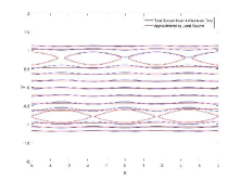
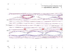
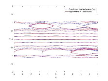
Figure 2: Lagrangian fluid trajectories of the learned meandering jet model (2.5)- (2.6) with 20 initial positions: The fluid motion in the deterministic basic model when noise is absent (left) is steady, with no exchange of fluid between the eddies and the jet stream. Under additive noise (middle) and multiplicative noise (right), there are fluid exchanges between eddies and the jet stream.

II.2 Mean residence time

In this subsection, we will consider stochastic quasigeostrophic meandering jet models, (2.1)- (2.2) and (2.3)-(2.4), to discover mean residence time by our approach.

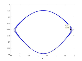
Figure 3: An eddy: $\sigma=0$ .

We take an eddy (FIG. 3) as the bounded domain $D$ (with boundary $\partial D$ composed with meander trough and crest).

The mean residence time $u(x,y)$ of the stochastic system (2.1)-(2.2) with additive noise for a trajectory starting in the eddy, satisfies the following elliptic partial differential equation as in (1.4)-(1.5):

$$\frac{1}{2}\sigma^{2}\triangle u+(-\psi_{y})u_{x}+(\psi_{x})u_{y}=-1,$$ (3.1)

$$u|_{\partial D}=0.$$ (3.2)

The mean residence time, as solution of this elliptic partial differential equation, is denoted by $u_{True}$. For the corresponding learned meandering jet model (2.5)- (2.6), with learned coefficients in Table I, we can also set up a similar elliptic partial differential equation for learned mean residence time $u_{Learn}$.

Similarly, the mean residence time $u(x,y)$ of the stochastic system (2.3)-(2.4) with multiplicative noise, for a trajectory starting in the eddy, satisfies the following elliptic partial differential equation as in (1.4)-(1.5):

$$\frac{1}{2}\sigma^{2}x^{2}u_{xx}+\frac{1}{2}\sigma^{2}y^{2}u_{yy}+(-\psi_{y})u_{x}+(\psi_{x})u_{y}=-1,$$ (3.3)

$$u|_{\partial D}=0.$$ (3.4)

The mean residence time, as solution of this elliptic partial differential equation, is denoted by $u_{True}$. For the corresponding learned meandering jet model (2.5)- (2.6), with learned coefficients in Table II, we can also set up a similar elliptic partial differential equation for learned mean residence time $u_{Learn}$.

We use a finite element code to solve the preceding elliptic differential equations to get mean residence time $u_{True}$ and $u_{Learn}$, for both additive and multiplicative noise cases. FIG. 4 shows the mean residence time $u_{Learn}$, as $u_{True}$ is barely distinguishable from $u_{Learn}$ when they are plotted together. Thus we compare the error between the maximal values of the mean residence times $u_{True}$ and $u_{Learn}$. In fact, the error of mean residence time between the learned system and the original system is $\mbox{error}(u)=\max_{(x,y)\in D}\|u_{Learn}-u_{True}\|=2.2142\times 10^{-4}$ for additive noise case, and $\mbox{error}(u)=\max_{(x,y)\in D}\|u_{Learn}-u_{True}\|=1.3\times 10^{-3}$ for multiplicative noise case.

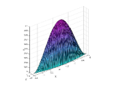
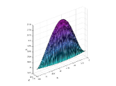
Figure 4: Learned mean residence time $u_{Learn}$ for stochastic system (2.5)-(2.6) in an eddy. Additive noise case is on the left, and multiplicative noise case is on the right.

II.3 Escape probability

We again take the eddy (FIG. 3) to be the bounded domain $D$ (with boundary $\partial D$ composed with meander trough (lower subboundary) and crest (upper subboundary)). For the stochastic meandering jet system (2.1)-(2.2) with additive noise, the escape probability $p(x,y)$ of a fluid particle, starting at $(x,y)$ in an eddy and escaping through a boundary component $\Gamma$ (either the trough or crest), satisfies the elliptic partial differential equation (1.6)-(1.8):

$$\frac{1}{2}\sigma^{2}\triangle p+(-\psi_{y})p_{x}+(\psi_{x})p_{y}=0,$$ (4.1)

$$p|_{\Gamma}=1,$$ (4.2)

$$p|_{\partial D\setminus\Gamma}=0.$$ (4.3)

For the corresponding learned meandering jet model (2.5)- (2.6), with learned coefficients in Table I, we can also set up a similar elliptic partial differential equation for the learned escape probability $p_{Learn}$.

Similarly, for the stochastic meandering jet system (2.3)-(2.4) with multiplicative noise, the escape probability $p(x,y)$ of a fluid particle, starting at $(x,y)$ in an eddy and escaping through a boundary component $\Gamma$ (either the trough or crest), satisfies the elliptic partial differential equation (1.6)-(1.8):

$$\frac{1}{2}\sigma^{2}x^{2}p_{xx}+\frac{1}{2}\sigma^{2}y^{2}p_{yy}+(-\psi_{y})p_{x}+(\psi_{x})p_{y}=0,$$ (4.4)

$$p|_{\Gamma}=1,$$ (4.5)

$$p|_{\partial D\setminus\Gamma}=0.$$ (4.6)

For the corresponding learned meandering jet model (2.5)- (2.6), with learned coefficients in Table II, we can also set up a similar elliptic partial differential equation for the learned escape probability $p_{Learn}$.

FIGs. 5-6 show the finite element solution for the learned escape probability $p_{Learn}$ alone, as $p_{True}$ is barely distinguishable from $p_{Learn}$ when they are plotted together. Thus we compare the error between the average escape probability values.

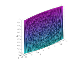
Figure 5: Learned escape probability $P_{Learn}$ for stochastic system (2.5)-(2.6) in an eddy, exiting from upper subboundary. Additive noise case is on the left, and multiplicative noise case is on the right.

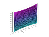
Figure 6: Learned escape probability $P_{Learn}$ for stochastic system (2.5)-(2.6) in an eddy, exiting from lower subboundary. Additive noise case is on the left, and multiplicative noise case is on the right.

For fluid particles initially uniformly distributed in $D$ (an eddy), we compute the average escape probability $P$ for particles leaving $D$ through the upper or lower subboundary $\Gamma$, given by $P=\frac{1}{D}\int\int_{D}p(x,y)dxdy$. The error of average escape probability, for fluid particles exiting fom $D$ through the upper subboundary, between the learned system and the original system is $\mbox{error}(P)=\|P_{Learn}-P_{True}\|=1.3949\times 10^{-5}$ both for additive noise and multiplicative noise cases. The error of the average escape probability, for particles leaving $D$ through the lower subboundary, between the learned system and the original system is $\mbox{error}(P)=\|P_{Learn}-P_{True}\|=7.4133\times 10^{-4}$ both for additive noise and multiplicative noise cases.

III Learning three dimensional stochastic dynamical systems

In this section, we will illustrate our method in two systems with additive noise. The first system is for a three dimensional stochastic linear oscillator. The second is the more complex stochastic Lorenz system. In these two examples, data from direct numerical simulations (as ‘observation data’) are used to discover mean residence time and escape probability.

III.1 A stochastic linear system

We consider a linear stochastic system

$$dx = (-0.1x-2y)dt+\sqrt{\epsilon}dB_{1},$$ (5.1)

$$dy = (2x-0.1y)dt+\sqrt{\epsilon}dB_{2},$$ (5.2)

$$dz = (-0.3z)dt+\sqrt{\epsilon}dB_{3},$$ (5.3)

where $\epsilon$ is the noise intensity (taken to be $0.9$ here), and $B_{1}(t)$, $B_{2}(t)$, $B_{3}(t)$ are three independent Brownian motions. With sample path data for this system, we try to discover the governing equation,

$$\dot{x} = \Theta\xi^{1},$$ (5.4)

$$\dot{y} = \Theta\xi^{2},$$ (5.5)

$$\dot{z} = \Theta\xi^{3}.$$ (5.6)

as in Brunton et al.Kutz but we use a stochastic basis. Here $\Theta$ is a set of basis functions and $\Xi=[\xi^{1},\xi^{2},\xi^{3}]$ are coefficients (or weights). As in Section 2, we collect data $(x(t_{i}),y(t_{i}),z(t_{i})),i=1,\cdots,20000$, from samplewise simulations of the original system (5.1)-(5.3), and construct a library $\Theta$ consisting of polynomial $\{1,x,y,z,\cdots,z^{4}\}$ and time derivatives of Brownian motions $\{dB_{1}/dt,dB_{2}/dt,dB_{3}/dt\}$. We then solve a regression problem to determine the weights $\xi^{k}=[\xi_{1}^{k},\cdots,\xi_{38}^{k}],k=1,2,3.$ See Table 3 and FIG. 7.

Table 3: Identified coefficients for discovering a three-dimensional stochastic linear system with basis functions. Sample paths of (5.1)-(5.3) with initial position $(1,1,1)^{T}$ are numerically generated, for $t\in[0,200]$ with stepsize $0.01$.

basis	$\dot{x}$	$\dot{y}$	$\dot{z}$
$1$	-3.9018726e-06	-2.5270553e-06	9.9621283e-06
$x$	-9.9972593e-02	2.0000178e+00	-6.9973977e-05
$y$	-1.9999463e+00	-9.9965198e-02	-1.3719725e-04
$z$	1.9721074e-04	1.2772392e-04	-3.0050351e-01
$x^{2}$	4.1955355e-05	2.7172467e-05	-1.0711898e-04
$xy$	-2.9428922e-06	-1.9059698e-06	7.5136920e-06
$xz$	1.2255057e-04	7.9370113e-05	-3.1289194e-04
$y^{2}$	2.4067948e-05	1.5587653e-05	-6.1449464e-05
$yz$	3.3875553e-04	2.1939567e-04	-8.6489908e-04
$z^{2}$	4.0214283e-03	2.6044858e-03	-1.0267374e-02
$x^{3}$	-1.1648871e-04	-7.5444137e-05	2.9741500e-04
$x^{2}y$	-2.3616373e-04	-1.5295190e-04	6.0296519e-04
$x^{2}z$	-8.2888236e-04	-5.3682726e-04	2.1162742e-03
$xy^{2}$	-1.1776806e-04	-7.6272713e-05	3.0068141e-04
$xyz$	3.5179026e-05	2.2783764e-05	-8.9817889e-05
$xz^{2}$	-1.8287612e-03	-1.1844007e-03	4.6691307e-03
$y^{3}$	-2.3525676e-04	-1.5236450e-04	6.0064954e-04
$y^{2}z$	-1.0099170e-03	-6.5407468e-04	2.5784856e-03
$yz^{2}$	-6.2014715e-03	-4.0163950e-03	1.5833386e-02
$z^{3}$	-1.2428487e-02	-8.0493336e-03	3.1731989e-02
$x^{4}$	-9.3740853e-05	-6.0711444e-05	2.3933595e-04
$x^{3}y$	-2.1022902e-06	-1.3615523e-06	5.3674957e-06
$x^{3}z$	7.5057766e-04	4.8611307e-04	-1.9163493e-03
$x^{2}y^{2}$	-1.2711976e-04	-8.2329355e-05	3.2455783e-04
$x^{2}yz$	1.8010661e-03	1.1664639e-03	-4.5984206e-03
$x^{2}z^{2}$	2.2180393e-03	1.4365174e-03	-5.6630223e-03
$xy^{3}$	-8.7412104e-06	-5.6612618e-06	2.2317761e-05
$xy^{2}z$	7.6527222e-04	4.9563003e-04	-1.9538669e-03
$xyz^{2}$	-3.0539398e-05	-1.9778900e-05	7.7972151e-05
$xz^{3}$	4.8388992e-05	3.1339224e-05	-1.2354512e-04
$y^{4}$	-3.2625868e-05	-2.1130207e-05	8.3299255e-05
$y^{3}z$	1.7990625e-03	1.1651663e-03	-4.5933050e-03
$y^{2}z^{2}$	2.2767938e-03	1.4745699e-03	-5.8130323e-03
$yz^{3}$	3.0332728e-03	1.9645050e-03	-7.7444488e-03
$z^{4}$	5.7423101e-03	3.7190182e-03	-1.4661070e-02
$dB1/dt$	9.4868476e-01	9.4448784e-07	-3.7233490e-06
$dB2/dt$	-1.8088277e-05	9.4867158e-01	4.6182372e-05
$dB2/dt$	4.2468852e-05	2.7505034e-05	9.4857487e-01

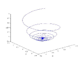
Figure 7: Trajectory of the three-dimensional stochastic linear system starting at $(1,1,1)^{T}$: The trajectory for the original system in blue curve (left) and for the learned system in red curve (right).

We take cuboid $D=[-2,2]\times[-2,2]\times[0,1]$, with boundary $\partial D$, containing a subboundary $\Gamma$ to be the surface $z=1$ (top boundary) or the surface $z=0$ (bottom boundary).

For the original system (5.1)-(5.3), the mean residence time $u$ (for solutions with initial points in $D$) and escape probability $p$ (for solutions exiting through a subboundary $\Gamma$) satisfy the elliptic partial differential equations (1.4)-(1.5) and (1.6)-(1.8), respectively. Hence,

$$\frac{1}{2}\epsilon\triangle u+(-0.1x-2y)u_{x}+(2x-0.1y)u_{y}+(-0.3z)u_{z} = -1,$$

$$u|_{\partial D} = 0.$$

$$\frac{1}{2}\epsilon\triangle p+(-0.1x-2y)p_{x}+(2x-0.1y)p_{y}+(-0.3z)p_{z} = 0,$$

$$p|_{\Gamma} = 1,$$

$$p|_{\partial D\setminus\Gamma} = 0.$$

These equations can also be solved by a finite element method to get the mean residence time $u_{True}$, and the escape probability $p_{True}$ and the average escape probability $P_{True}$.

For the learned model (5.4)-(5.6), we also have similar elliptic partial differential equations for the mean residence time $u_{Learn}$, the escape probability $p_{Learn}$ and the average escape probability $P_{Learn}$.

The mean residence time $u(x,y,z)$ of the learned model is shown in FIG. 8. It is barely distinguishable from the mean residence time for the original system and we thus do not show the latter. Instead, we compute the error (using 20000 uniformly distributed points in $D$) between the maximal values of mean residence time for the learned and original systems: $\mbox{error}(u)=\max_{(x,y,z)\in D}\|u_{Learn}-u_{True}\|=3.7495\times 10^{-4}$.

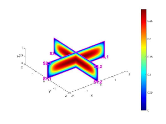
Figure 8: Learned mean residence time $u_{Learn}$ for the learned linear stochastic system (5.4)-(5.6), as viewed in two slices.

The escape probability $p(x,y,z)$ of the learned system is shown in FIG. 9. It is barely distinguishable from the escape probability for the original system and we thus do not show the latter. Instead, we calculate the error between the average escape probability values of the learned system and original system is $\mbox{error}(P)=\|P_{Learn}-P_{True}\|=9.9478\times 10^{-7}$ (escaping from the top boundary) and $\mbox{error}(P)=\|P_{Learn}-P_{True}\|=1.0783\times 10^{-4}$ (escaping from the bottom boundary).

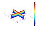
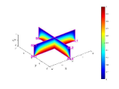
Figure 9: Learned escape probability for the learned linear stochastic system (5.4)-(5.6): escaping from top surface (left) and bottom surface (right). Two slices are shown for each subfigure.

III.2 Lorenz system with random noises

We consider a stochastic Lorenz system Kutz :

$$dx = \sigma(y-x)dt+\sqrt{\epsilon}dB_{1},$$ (5.7)

$$dy = (\rho x-xz-y)dt+\sqrt{\epsilon}dB_{2},$$ (5.8)

$$dz = (xy-\beta z)dt+\sqrt{\epsilon}dB_{3},$$ (5.9)

where $\sigma=10$, $\beta=\frac{8}{3}$, $\rho=28$ are standard parameters, and $B_{1}(t)$, $B_{2}(t)$, $B_{3}(t)$ are independent scalar Brownian motions. We take $\epsilon=0.9$ in the following computations.

As before, a learned model is identified in the following form

$$\dot{x} = \Theta\xi^{1},$$ (5.10)

$$\dot{y} = \Theta\xi^{2},$$ (5.11)

$$\dot{z} = \Theta\xi^{3},$$ (5.12)

where $\Theta$ is a set of basis function consisting of polynomials in $(x,y,z)$ up to fourth order and time derivatives of three independent Brownian motions. Then we solve a regression problem to determine the weights $\Xi=[\xi^{1},\xi^{2},\xi^{3}]$; see Table 4.

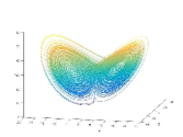
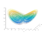
Figure 10: One trajectory starting at $(x,y,z)^{T}=(-8,7,27)^{T}$: for the original Lorenz system (left), and for the learned Lorenz system with basis in Table 4 (right).

Table 4: Identified Lorenz system with basis functions. The sample paths data are numerically generated by solving (5.7)-(5.9) with initial position $(-8,7,27)^{T}$, for $t\in[0,200]$ with stepsize $0.01$.

basis	$\dot{x}$	$\dot{y}$	$\dot{z}$
$1$	7.5197692e-03	3.3528379e-03	-1.3696228e-02
$x$	-1.0008895e+01	2.7996034e+01	1.6200350e-02
$y$	1.0004690e+01	-9.9790907e-01	-8.5413967e-03
$z$	-2.7045815e-03	-1.2058912e-03	-2.6617406e+00
$x^{2}$	-4.5633362e-04	-2.0346537e-04	8.3114908e-04
$xy$	-6.6325912e-04	-2.9572721e-04	1.0012080e+00
$xz$	1.0139842e-03	-9.9954790e-01	-1.8468331e-03
$y^{2}$	4.1804010e-04	1.8639145e-04	-7.6140269e-04
$yz$	-5.5344389e-04	-2.4676391e-04	1.0080221e-03
$z^{2}$	3.0860393e-04	1.3759717e-04	-5.6207972e-04
$x^{3}$	3.8011238e-05	1.6948062e-05	-6.9232255e-05
$x^{2}y$	-5.6250702e-05	-2.5080489e-05	1.0245294e-04
$x^{2}z$	4.3954760e-05	1.9598100e-05	-8.0057566e-05
$xy^{2}$	1.1078797e-05	4.9397009e-06	-2.0178509e-05
$xyz$	1.6070760e-05	7.1654662e-06	-2.9270684e-05
$xz^{2}$	-3.4384030e-05	-1.5330800e-05	6.2625795e-05
$y^{3}$	4.3084220e-06	1.9209952e-06	-7.8471997e-06
$y^{2}z$	-1.1913783e-05	-5.3119961e-06	2.1699322e-05
$yz^{2}$	2.0432252e-05	9.1101240e-06	-3.7214544e-05
$z^{3}$	-1.3645677e-05	-6.0841951e-06	2.4853729e-05
$x^{4}$	2.4710563e-07	1.1017693e-07	-4.5006900e-07
$x^{3}y$	-1.5318615e-06	-6.8301077e-07	2.7900756e-06
$x^{3}z$	-6.0616355e-07	-2.7027001e-07	1.1040438e-06
$x^{2}y^{2}$	1.9963786e-06	8.9012488e-07	-3.6361297e-06
$x^{2}yz$	1.1588151e-06	5.1668065e-07	-2.1106228e-06
$x^{2}z^{2}$	-1.0342002e-06	-4.6111863e-07	1.8836538e-06
$xy^{3}$	-7.4783630e-07	-3.3343761e-07	1.3620812e-06
$xy^{2}z$	-2.2736871e-07	-1.0137684e-07	4.1412091e-07
$xyz^{2}$	2.5757823e-07	1.1484635e-07	-4.6914341e-07
$xz^{3}$	3.3732532e-07	1.5040317e-07	-6.1439179e-07
$y^{4}$	-2.9520887e-09	-1.3162472e-09	5.3768245e-09
$y^{3}z$	-1.1011727e-07	-4.9097963e-08	2.0056350e-07
$y^{2}z^{2}$	-6.2710697e-08	-2.7960805e-08	1.1421893e-07
$yz^{3}$	-2.3846556e-07	-1.0632459e-07	4.3433230e-07
$z^{4}$	2.0349814e-07	9.0733672e-08	-3.7064394e-07
$dB1/dt$	9.4581495e-01	-1.2789082e-03	5.2242963e-03
$dB2/dt$	-3.1279105e-03	9.4728866e-01	5.6970599e-03
$dB3/dt$	3.4942944e-03	1.5580003e-03	9.4231892e-01

A single trajectory of this stochastic system with initial condition $(x,y,z)^{T}=(-8,7,27)^{T}$ is shown in FIG. 10 (left), together with the same trajectory captured by the learned model in FIG. 10 (right).

For the stochastic Lorenz system, we take a cuboid $D$ to be either $D_{1}=[-9,-8]\times[-9,-8]\times[27,28]$ containing the left saddle as left residence region, or $D_{2}=[8,9]\times[8,9]\times[27,28]$ containing the right saddle as the right residence region. Then mean residence time and escape probability satisfy the following elliptic partial differential equations, respectively:

$$\frac{1}{2}\varepsilon\triangle u+(\sigma(y-x))u_{x}+(\rho x-xz-y)u_{y}+(xy-\beta z)u_{z} = -1,$$

$$u|_{\partial D_{i}}=0,~{}i=1,2.$$

$$\frac{1}{2}\varepsilon\triangle p+(\sigma(y-x))p_{x}+(\rho x-xz-y)p_{y}+(xy-\beta z)p_{z} = 0,$$

$$p|_{\Gamma} = 1,$$

$$p|_{\partial D_{i}\setminus\Gamma}=0,~{}i=1,2.$$

The finite element numerical solutions to these partial differential equations are denoted by $u_{True}$ and $p_{True}$.

For the learned Lorenz system (5.10)-(5.12), with basis and coefficients in Table 4, we can also set up the partial differential equations for the learned mean residence time $u_{Learn}$, and the learned escape probability $p_{Learn}$ together with the average escape probability $P_{Learn}$.

The learned mean residence time $u$ of the learned Lorenz system (5.10)-(5.12) is shown in FIG. 11. The maximal mean residence time in the left region $D_{1}$ is $u_{Learn}(D_{1})=0.1238$, while the maximal mean residence time in the right region $D_{2}$ is $u_{Learn}(D_{2})=0.1236$. Then we compute the error of maximal mean residence time between the learned and the original systems, $\mbox{error}(u(D_{1}))=\max_{(x,y,z)\in D_{1}}\|u_{Learn}-u_{True}\|=1.0023\times 10^{-4}$, and $\mbox{error}(u(D_{2}))=\max_{(x,y,z)\in D_{2}}\|u_{Learn}-u_{True}\|=1.2284\times 10^{-5}$.

We take $\Gamma$ to be each surface of the region. The learned escape probability $p_{Learn}$ of particles exiting through each surface $\Gamma$ of left and right regions are showed in FIG. 12 - 13, respectively, and the average escape probability of left region is $P_{Learn}(L_{1})=0.1065$ (from $x=-9$), $P_{Learn}(L_{2})=0.1167$ (from $x=-8$), $P_{Learn}(L_{3})=0.0955$ (from $y=-9$), $P_{Learn}(L_{4})=0.3485$ (from $y=-8$), $P_{Learn}(L_{5})=0.2343$ (from $z=27$), $P_{Learn}(L_{6})=0.1244$ (from $z=28$). Similarly, the average escape probability of right region is $P_{Learn}(R_{1})=0.1161$ (from $x=8$), $P_{Learn}(R_{2})=0.1061$ (from $x=9$), $P_{Learn}(R_{3})=0.3469$ (from $y=8$), $P_{Learn}(R_{4})=0.0947$ (from $y=9$), $P_{Learn}(R_{5})=0.2367$ (from $z=27$), $P_{Learn}(R_{6})=0.1264$ (from $z=28$).

Moreover, for example, we compute the error of the average escape probability between the learned and the original systems only for two cases, $\mbox{error}(P)(L4)=\|P_{Learn}(L4)-P_{True}(L4)\|=6.5838\times 10^{-3}$, and $\mbox{error}(P)(R3)=\|P_{Learn}(R3)-P_{True}(R3)\|=6.431\times 10^{-3}$. (L4)

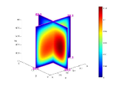
Figure 11: Learned mean residence time of the learned Lorenz system (5.10)-(5.12) in $D_{1}$ (left) and $D_{2}$ (right): Two slices are shown for each subfigure.

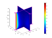
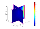
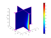
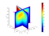
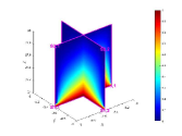
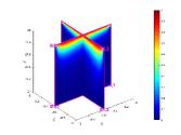
Figure 12: Learned escape probability of the learned Lorenz system (5.10)-(5.12) in left region $D_{1}$ exiting from a subboundary $\Gamma$: surface $x=-9$ (upper left), $x=-8$ (upper middle), $y=-9$ (upper right), $y=-8$ (lower left), $z=27$ (lower middle), and $z=28$ (lower right). Two slices are shown for each subfigure.

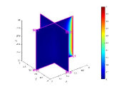
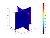
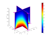
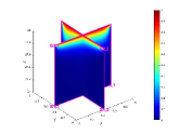
Figure 13: Learned escape probability of the learned Lorenz system (5.10)-(5.12) in right region $D_{2}$ exiting from a subboundary $\Gamma$: surface $x=8$ (upper left), $x=9$ (upper middle), $y=8$ (upper right), $y=9$ (lower left), $z=27$ (lower middle), and $z=28$ (lower right). Two slices are shown for each subfigure.

IV Conclusion

In summary, we have demonstrated a new data-driven method to determine dynamical quantities, mean residence time and escape probability, based on sample path data of complex systems, as long as these systems are modeled by stochastic differential equations.

A novelty of this method is that it contains noise terms (in terms of Brownian motions) in the basis, in order to discover the governing stochastic differential equation. With the governing stochastic differential equation as the model for the sample path data, we can then compute the mean residence time and escape probability, which are deterministic quantities that carry significant dynamical information.

This method combines machine learning tools (i.e., extracting governing stochastic differential equations from data) and stochastic dynamical systems techniques (i.e., understanding random phenomena with deterministic quantities), to provide an efficient approach in examining stochastic dynamics from data.

To demonstrate that our method is effective, we have illustrated it on several stochastic systems with Brownian motions. It is expected to be applicable to data sets from other stochastic dynamical systems.

- (1) L. Arnold, Random dynamical systems, Springer, New York, 1998.
- (2) L. Arnold, Stochastic differential equations: theory and applications. Wiley-Interscience [John Wiley & Sons], New York-London-Sydney, 1974. xvi+228 pp.
- (3) D. Biegie, A. Lenoad, S. Wiggins, The dynamics associated with the chaotic tangles of two-dimensional quasiperiodic vector fields: Theory and applications. Nonlinear Phenomena in Atmospheric and Oceanic Science. 40 (1992), 47–138.
- (4) A. S. Bower, T.Rossby, Evidence of cross-frontal exchange processes in the Gulf stream based on isopycnal RAFOS float data. Journal of Physical Oceanography 19 (1989), 1177–1190.
- (5) A.S.Bower, A simple kinematic mechanism for mixing fluid parcels across a meandering jet. Journal of Physical Oceanography 21 (1991), 173–180.
- (6) J. Duan, S. Wiggins, Fluid exchange across a meandering jet with quasiperiodic variability. Journal of Physical Oceanography 26(1995),1176-1188.
- (7) J. R. Brannan, J. Duan, V. J. Ervin, Escape probability, mean residence time and geophysical fluid particle dynamics. Physica D 133 (1999), 23–33.
- (8) D. del-Castillo-Negrete, P. J. Morris, Chaotic transport by Rossby waves in shear flow. Physica Fluid A 5 (1993), 948–965.
- (9) J. Duan, An introduction to stochastic dynamics. Cambridge University Press, New York.(2015).
- (10) T. Gao and J. Duan, Quantifying model uncertainty in dynamical systems driven by non-Gaussian Lévy stable noise with observations on mean exit time or escape probability. Commun Nonlinear Sci Numer Simulat 39 (2016)1-6.
- (11) L. J. Pratt, M. S. Lozier, N. Beliakova, Parcel trajetories in quasigeostrophic jets: neutral models.Journal of Physical Oceanography 25(1995), 1451-1466.
- (12) P. Miller, C.K.R.T.Jones, G. Haller, L. Pratt,, Chaotic mixing across oceanic jets.Proceeding AIP 275(1996), 591-604.
- (13) J. Pedlosky, Geophysical fluid dynamics, 2nd ed. Springer, New York. (1987).
- (14) L. Perko, Differential equations and dynamical systems, 3rd ed. Springer, New York. (2001).
- (15) R. M. Samelson, Fluid exchange across a meandering jet. Journal of Physical Oceanography 22(4) (1992), 431–440.
- (16) R. M. Samelson, Stochastic forced current fluctuatuations in vertical shear and over topography . J. Geogaphy Res. 94 (1989), 8207–8215.
- (17) B. Oksendal, Stochastic differntial equations. 6th ed. Springers, New York.(2005).
- (18) S. Zhang, G. Lin, Robust data-driven discovery of governing physical laws with error bars.Proceedings of the Royal Society A: Mathematical, Physical and Engineering Sciences 474(2018), 1-21.
- (19) D. J. Higham, An algorithmic introduction to numerical simulation of stochastic differential equations. SIAM Rev 43(3) (2001), 525–546.
- (20) S. L. Brunton, J. L. Proctor, J. N. Kutz, Discovering governing equaitions from data by sparse identification of nonlinear dynamical systems.Proceedings of the National Academy of Sciences of the United States of America 113(15)(2016), 3932-3937.
- (21) L. Dunker, G. Bohner, J. Boussard, M. Sahani, Learning interpretable continuous-time models of latent stochastic dynamical systems.Stat 113(15)(2019), 3932-3937.
- (22) C. Cotter, D. Crisan, D. D. Holm, W. Pan, I.Shevchenko, Modeling uncertainty using circulation-preserving stochastic transport noise in a 2-layer quasi-geostrohic model.Physics flu-dyn 113(15)(2018), 1-37.
- (23) M. Crosskey, M. Maggioni, ATLAS: A geometric approach to learning high-dimensional stochastic systems near manifolds.Multiscale Modeling and Simulation 15(1)(2017), 110-156.