Choked accretion: from radial infall to bipolar outflows by breaking spherical symmetry

Abstract

Steady state, spherically symmetric accretion flows are well understood in terms of the Bondi solution. Spherical symmetry however, is necessarily an idealized approximation to reality. Here we explore the consequences of deviations away from spherical symmetry, first through a simple analytic model to motivate the physical processes involved, and then through hydrodynamical, numerical simulations of an ideal fluid accreting onto a Newtonian gravitating object. Specifically, we consider axisymmetric, large-scale, small amplitude deviations in the density field such that the equatorial plane is over dense as compared to the polar regions. We find that the resulting polar density gradient dramatically alters the Bondi result and gives rise to steady state solutions presenting bipolar outflows. As the density contrast increases, more and more material is ejected from the system, attaining speeds larger than the local escape velocities for even modest density contrasts. Interestingly, interior to the outflow region, the flow tends locally towards the Bondi solution, with a resulting total mass accretion rate through the inner boundary choking at a value very close to the corresponding Bondi one. Thus, the numerical experiments performed suggest the appearance of a maximum achievable accretion rate, with any extra material being ejected, even for very small departures from spherical symmetry.

1 Introduction

The accretion of fluids towards gravitational objects is a topic of general interest in astrophysics, as such phenomena underpin the physics of large classes of systems (Hawley et al., 2015). Notably, the ubiquitous jets observed from Young Stellar Objects (YSOs) to Gamma Ray Bursts (GRBs) and Active Galactic Nuclei (AGN), are fuelled by the accretion of gas on to massive objects. Although the detailed physics of accretion problems is complex, including the effects of rotation, magnetic fields, non-ideal fluids and mixing, to name but a few (Pudritz et al., 2007; Tchekhovskoy, 2015; Jafari, 2019), the availability of simplified analytic solutions where the salient physical ingredients can be transparently traced, has always provided valuable insights and well understood limiting cases for the analysis of these systems.

The first analytic solution to such an accretion problem was the Newtonian spherically symmetric model of Bondi (1952), with the corresponding extension to general relativity by Michel (1972). In both cases, the authors assumed stationariness, spherical symmetry and zero angular momentum for the infalling material, which was in turn described as an ideal fluid.

On the other hand, the origin of jets is typically understood in connection with accretion disc models, where the geometry very strongly deviates from spherical symmetry. In these, rotation and small-scale magnetic fields are considered as fundamental for the stability and evolution of the disc (Shakura & Sunyaev, 1973; Balbus & Hawley, 1991), while the interplay of these with a large-scale magnetic field is thought to be responsible for the launching and subsequent collimation of the jet (Hawley et al., 2015). This so-called magneto-rotational mechanism has been studied both at a Newtonian level (Lovelace, 1976; Blandford, 1976; Blandford & Payne, 1982) and in general relativity when a central black hole is involved (Blandford & Znajek, 1977).

The viability of the magneto-rotational mechanism for launching powerful jets has been successfully demonstrated by means of magneto-hydrodynamic (MHD) numerical simulations. This has been done at a non-relativistic level for jets associated to YSOs (Casse & Keppens, 2002), as well as with comprehensive, general relativistic-MHD simulations of accretion discs around spinning black holes (Semenov et al., 2004; Qian et al., 2018; Sheikhnezami & Fendt, 2018; Liska et al., 2019).

The similarity of jets across a vast range of astrophysical scales, from quasars to micro-quasars (e.g. Mirabel & Rodríguez, 1994), along with open questions regarding the matter content of relativistic jets (Hawley et al., 2015) or the link between the accretion disc and the acceleration process (Romero et al., 2017), might hint towards the presence in some cases of more simple outflow-producing mechanisms based on hydrodynamical physics. Moreover, it is clear that if some kind of universal mechanism underlies all astrophysical jets, then it can not rely on the central accretor being a black hole.

Hydrodynamical models have been introduced for collimating and accelerating jets, in the context of AGNs (Blandford & Rees, 1974) and of YSOs (specifically H-H objects as studied by Canto & Rodriguez, 1980). On the other hand, a purely hydrodynamical mechanism, where a small amplitude density gradient on the inflow boundary conditions yields and inflow/outflow steady state solution, was introduced by Hernandez et al. (2014) based on an analytic perturbation analysis of the hydrodynamic equations for an isothermal fluid.

In Hernandez et al. (2014), the authors consider an originally radial accretion flow that becomes increasingly dense as the fluid approaches the central accretor. As the authors assume that this flow originates from the inner walls of a disc-like configuration, there is a certain degree of inhomogeneity in the density field, with the polar regions being less dense than the disc plane. As a result of this density inhomogeneity, on approaching the central regions the geometrical focusing of the accreted material results in a pressure gradient that deviates some of the fluid elements from their infall trajectories and expels them from the central region along a bipolar outflow. Within this scenario, the resulting bipolar outflow is neither accelerated to large Mach numbers, nor collimated as a proper jet.

Following on from Hernandez et al. (2014), in this work we extend the previous results by considering more realistic adiabatic indices for the infalling material. The problem can no longer be treated analytically, so we implement full hydrodynamical numerical simulations using the free GPL hydrodynamical code aztekas (Olvera & Mendoza, 2008; Aguayo-Ortiz et al., 2018).

We have found with these simulations a flux-limited accretion mode, in which the total mass infall rate onto the central accretor is limited by a fixed value. This value coincides very closely with the mass accretion rate of the spherically symmetric Bondi solution. Whenever the incoming accretion flow surpasses this threshold value, the excess flow is redirected by a density gradient and expelled through the poles. Since the incoming accretion flow is jamming at a gravitational bottleneck, we refer to this ejection mechanism as choked accretion.

With the numerical simulations presented in this work we recover the main result of Hernandez et al. (2014) that a large scale, small amplitude inhomogeneity in the density field can lead to the onset of a bipolar outflow as a generic result. The choked accretion model can then be viewed as a transition bridge between the spherically symmetric condition treated by Bondi and Michel, where no outflows appear, and the disc geometries of the jet-generating models mentioned above.

In a separate work, Tejeda et al. (2019), we are proposing a full-analytic, general relativistic model of the choked accretion mechanism. This analytic model describes an ultra relativistic gas with a stiff equation of state (see Petrich et al., 1988) and is based on the conditions of steady state, axisymmetry and irrotational flow. As shown by Tejeda (2018), the non-relativistic limit of such a model corresponds to an incompressible fluid in Newtonian hydrodynamics. With this motivation in mind, we present in this article a simple analytic model of an incompressible fluid.

The remainder of the paper is organized as follows. In Section 2, we present a simple analytic model of the choked accretion that leads to an inflow/outflow configuration. Section 3 presents the hydrodynamical simulations used to extend this model to more general conditions, allowing for a range of plausible adiabatic indices. The code is validated and tested in the spherically symmetric case, where steady state solutions accurately tracing the corresponding Bondi ones are recovered. In Section 4 we analyse the results obtained and discuss the applicability of the choked accretion mechanism in astrophysical settings. Finally, in Section 5 we present our conclusions.

2 Analytic model

In order to present a simple model where the physics leading from the breakage of spherical symmetry to the establishing of an outflow can be traced transparently, in this section we discuss an analytic model of choked accretion. Following Tejeda (2018), this model is based on an incompressible fluid under the approximations of steady state, axisymmetry and irrotational flow.

This model can be considered as complementary to the perturbation analysis presented in Hernandez et al. (2014), where isothermal conditions were assumed, and which shows that a spherically symmetric flow onto a point mass is in fact unstable towards the development of the outflow phenomenology discussed here, as soon as a slight perturbation to spherical symmetry is introduced in the inflow conditions.

Under the irrotational flow condition, the fluid’s velocity field can be obtained as the gradient of a velocity potential $\Phi$ (i.e. $\vec{v}=\nabla\Phi$). For an incompressible fluid, this means that $\Phi$ has to be a solution to the Laplace equation $\nabla^{2}\Phi=0$. Adopting spherical coordinates and imposing the axisymmetry condition, we know that a general solution for $\Phi$ is given by (Currie, 2003)

$$\Phi=\sum_{n=0}^{\text{\tiny$\infty$ }}\left(A_{n}\,r^{n}+B_{n}\,r^{-(n+1)}\right)P_{n}(\cos\theta),$$ (2.1)

where $A_{n}$ and $B_{n}$ are constant coefficients and $P_{n}(\cos\theta)$ is the Legendre polynomial of degree $n$.

The lowest order solution that describes both accretion onto a central object and an axisymmetric, bipolar outflow has as only non-vanishing coefficients $B_{0}$ and $A_{2}$. Let us re-parametrize these two coefficients as $B_{0}=\alpha$, $A_{2}=\alpha/(2\,\mathcal{S}^{3})$, and write the solution as

$$\Phi=\frac{\alpha}{r}\left[1+\frac{r^{3}}{4\,\mathcal{S}^{3}}(3\cos^{2}\theta-1)\right],$$ (2.2)

which leads to the velocity field

$$\frac{\mathrm{d}r}{\mathrm{d}t}=-\frac{\alpha}{r^{2}}\left[1-\frac{r^{3}}{2\,\mathcal{S}^{3}}\left(3\cos^{2}\theta-1\right)\right],$$ (2.3)

$$\frac{\mathrm{d}\theta}{\mathrm{d}t}=-\frac{3\,\alpha\,\sin\theta\,\cos\theta}{2\,\mathcal{S}^{3}}.$$ (2.4)

This velocity profile has the same dependence on the polar angle as the one obtained for the isothermal hydrodynamic solutions of Hernandez et al. (2014), which are also given in terms of Legendre polynomials.

The parameter $\mathcal{S}$ is related to the location of the stagnation point, as from equations (2.3) and (2.4) we see that the points ($r=\mathcal{S}$, $\theta=0$) and ($r=\mathcal{S}$, $\theta=\pi$) correspond to the stagnation points of the flow. In Figure 1 we show an example of the resulting streamlines.

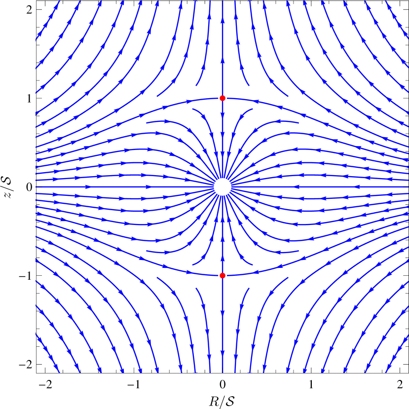
Figure 1: Streamlines of the incompressible analytic model showing an inner quasi-spherical accretion region, and polar stagnation points beyond which a polar outflow solution results. The red dots indicate the location of the stagnation points along the symmetry axis. The axes correspond to the usual cylindrical coordinates $R=r\,\sin\theta$, $z=r\,\cos\theta$.

On the other hand, the parameter $\alpha$ is related to the total accretion rate onto the central object in the following way

$$\dot{M}=-2\pi\int_{0}^{\pi}\rho\,\frac{\mathrm{d}r}{\mathrm{d}t}\,r^{2}\sin\theta\,\mathrm{d}\theta=4\pi\rho\,\alpha,$$ (2.5)

that is

$$\alpha=\frac{\dot{M}}{4\pi\rho}.$$ (2.6)

At this point $\dot{M}$ can have any arbitrary value. For the choked accretion model, we shall assume that $\dot{M}$ is given by the Bondi accretion rate, i.e.

$$\alpha=\frac{\dot{M}_{\mathrm{B}}}{4\pi\rho}=\frac{1}{4}\frac{(\mathrm{G}M)^{2}}{a{\text{\tiny$\infty$ }}^{3}}\left(\frac{2}{5-3\,\gamma}\right)^{\frac{5-3\,\gamma}{2(\gamma-1)}},$$ (2.7)

where $M$ is the mass of the central accretor, $\gamma$ the adiabatic index of the fluid and $a{\text{\tiny$\infty$ }}$ the speed of sound far away from the central object.

Let us consider that the flow is continuously being injected from a sphere of radius $\mathcal{R}$ that we shall refer to as the injection sphere. Provided that $\mathcal{S}<\mathcal{R}$, from equation (2.3) we see that the radial velocity changes sign at

$$\cos\theta_{0}=\sqrt{\frac{1}{3}\left(1+2\,\frac{\mathcal{S}^{3}}{\mathcal{R}^{3}}\right)}.$$ (2.8)

More specifically, the flow is characterized by an inflow/outflow geometry, with inflow ($\dot{r}<0$) across the equatorial belt defined by $\theta_{0}<\theta<\pi-\theta_{0}$ and outflow ($\dot{r}>0$) across the polar caps defined by $\theta<\theta_{0}$ and $\theta>\pi-\theta_{0}$.

We can calculate now the mass injection rate across the sphere of radius $\mathcal{R}$ as

$$\begin{split}\dot{M}_{\mathrm{in}}&=-4\pi\int_{\theta_{0}}^{\pi/2}\rho\,\frac{\mathrm{d}r}{\mathrm{d}t}\,\mathcal{R}^{2}\sin\theta\,\mathrm{d}\theta,\\ &=4\pi\rho\,\alpha\,\frac{\mathcal{R}^{3}}{\mathcal{S}^{3}}\left[\frac{1}{3}\left(1+2\,\frac{\mathcal{S}^{3}}{\mathcal{R}^{3}}\right)\right]^{3/2}.\end{split}$$ (2.9)

Similarly, we define the mass ejection rate leaving this same sphere as

$$\begin{split}\dot{M}_{\mathrm{ej}}&=4\pi\int_{0}^{\theta_{0}}\rho\,\frac{\mathrm{d}r}{\mathrm{d}t}\,\mathcal{R}^{2}\sin\theta\,\mathrm{d}\theta,\\ &=\dot{M}_{\mathrm{in}}-\dot{M}.\end{split}$$ (2.10)

Note that if $\mathcal{S}\geq\mathcal{R}$ then $\dot{M}_{\mathrm{in}}=\dot{M}$ and $\dot{M}_{\mathrm{ej}}=0$.

Finally, an expression for the streamlines can be found by combining equations (2.3) and (2.4) as

$$\frac{\mathrm{d}r}{\mathrm{d}\theta}=\frac{2\,\mathcal{S}^{3}-r^{3}\left(3\cos^{2}\theta-1\right)}{3\,r^{2}\sin\theta\,\cos\theta},$$ (2.11)

which can be integrated to give

$$r=S\left(2\frac{\Psi-\cos\theta}{\cos\theta\,\sin^{2}\theta}\right)^{1/3},$$ (2.12)

where $\Psi$ is an integration constant (stream function). From this expression we see that the streamlines corresponding to $\Psi=\pm 1$ are the only ones that arrive at the stagnation points located at $(\mathcal{S},\,0)$ and $(\mathcal{S},\,\pi)$, respectively. On the other hand, all of the streamlines with $|\Psi|<1$ accrete onto the central object while those with $|\Psi|>1$ escape along the bipolar outflow.

3 Numerical simulations

The simple toy model presented in the previous section is clearly limited by the assumption of an incompressible fluid. In this section we relax this condition and use instead full-hydrodynamic numerical simulations of a polytropic fluid obeying

$$P=K\,\rho^{\gamma},$$ (3.1)

where $P$ is the fluid pressure and $K=\mathrm{const.}$ In this work we consider three different values for the adiabatic index, namely $\gamma=1$ corresponding to an isothermal fluid, $\gamma=4/3$ describing a gas composed of relativistic particles, and $\gamma=7/5$ corresponding to the adiabatic index of a diatomic gas.

In order to capture the basic premise on which the mechanism of choked accretion operates, i.e. breaking spherical symmetry by introducing a small density contrast between the equator and the poles, here we parametrize this anisotropy by imposing the following density profile as boundary condition at the injection sphere ($r=\mathcal{R}$)

$$\rho(\theta)=\rho_{0}\left(1-\delta\cos^{2}\theta\right),$$ (3.2)

where $\rho_{0}$ is an arbitrary value that we set as the density unit and $\delta$ is the density contrast between the equator and the poles defined as

$$\delta=1-\frac{\rho(0)}{\rho(\pi/2)}.$$ (3.3)

We study this problem by means of numerical simulations performed with the hydrodynamical code aztekas. This code numerically solves the inviscid Euler equations in a conservative form,

$$\frac{\partial\rho}{\partial t}+\nabla\cdot\left(\rho\mathbf{v}\right)=0,$$ (3.4)

$$\frac{\partial\left(\rho\mathbf{v}\right)}{\partial t}+\nabla\cdot\left(\rho\mathbf{v}\otimes\mathbf{v}\right)+\nabla P=-\rho\frac{\mathrm{G}M}{r^{2}}\hat{r},$$ (3.5)

$$\frac{\partial E}{\partial t}+\nabla\cdot\left[\mathbf{v}\left(E+P\right)\right]=-\rho\frac{\mathrm{G}M}{r^{2}}\mathbf{v}\cdot\hat{r},$$ (3.6)

with $\mathbf{v}$ the fluid velocity vector and $E$ the total energy density defined as

$$E=\frac{1}{2}\rho|\mathbf{v}|^{2}+\epsilon,$$ (3.7)

where $\epsilon$ is the internal energy density. From equation (3.1), together with the first law of thermodynamics for an ideal gas, we can close this system of equations with the following equation of state that relates the pressure to the internal energy density

$$\epsilon=\frac{P}{\gamma-1}.$$ (3.8)

The equations (3.4)-(3.8) are spatially discretized using a finite volume scheme together with a High Resolution Shock Capturing (HRSC) method, that uses a second order piecewise linear reconstructor (MC) and the HLL (Harten et al., 1983) approximate Riemann solver to compute the numerical fluxes. The time evolution of these equations is calculated using a second order total variation diminishing Runge-Kutta time integrator (RK2) (Shu & Osher, 1988), with a Courant factor of 0.25.

Since the density profile in equation (3.2) is independent of the azimuthal angle, we assume that the problem retains symmetry with respect to both the polar axis (axisymmetry) and the equatorial plane (north-south symmetry). Hence, for the numerical simulations we adopt a two-dimensional spherical domain consisting of a uniform polar grid on $\theta\in[0,\pi/2]$ and a exponential radial grid with $r\in[\mathcal{R}_{\rm acc},\,\mathcal{R}]$, computed as

$$r_{i}=\mathcal{R}_{\rm acc}+{\rm exp}\left(\frac{\ln(\mathcal{R}-\mathcal{R}_{\rm acc})i}{N_{r}}\right),$$ (3.9)

where $\mathcal{R}_{\rm acc}$ is the radius of the inner boundary. As fiducial values for the numerical resolution we adopt $N_{r}=N_{\theta}=150$, while for the radial boundaries we take $\mathcal{R}_{\rm acc}=0.1\,r_{\mathrm{B}}$ and $\mathcal{R}=10\,r_{\mathrm{B}}$, where $r_{\mathrm{B}}=\mathrm{G}M/a^{2}_{\infty}$ is the Bondi radius. The code uses $r_{\mathrm{B}},\ a{\text{\tiny$\infty$ }}$ and $t_{\mathrm{B}}=r_{\mathrm{B}}/a{\text{\tiny$\infty$ }}$ as units of length, velocity and time, respectively.

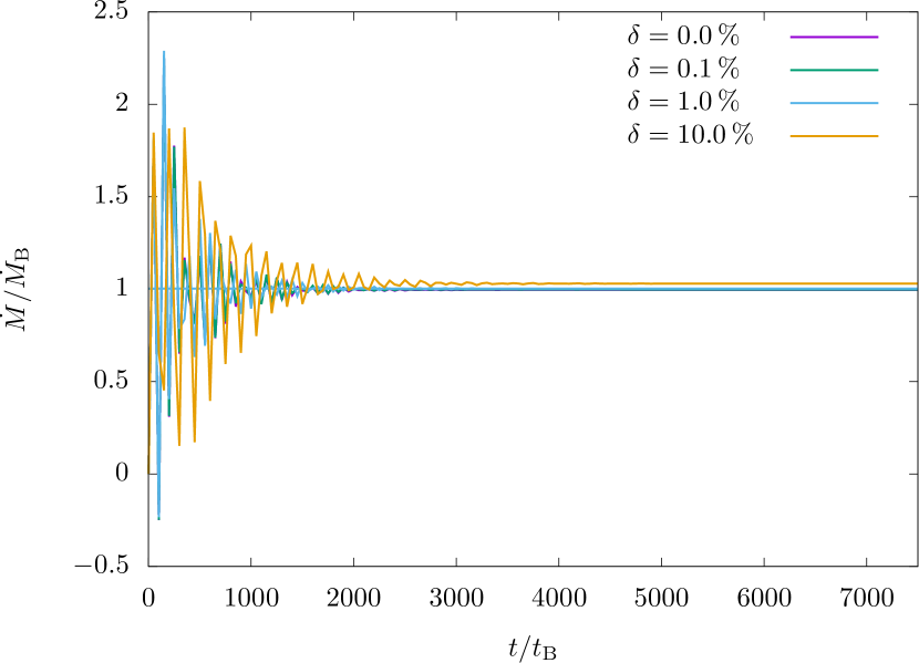
Figure 2: Mass accretion rate as a function of time for the four values of the density contrast $\delta$ in the case $\gamma=4/3$ (similar results were obtained for the other two values of $\gamma$). There is a clear convergence towards a steady state solution.

3.1 Initial and boundary conditions

We performed different simulations using three values of the adiabatic index $\gamma=1,\,4/3,\,7/5,$ and four values of the density contrast $\delta=0,\,0.1\%,\,1\%$, and 10$\%$. As boundary conditions, we set free-outflow from the grid at $\mathcal{R}_{\rm acc}$ (i.e. free inflow towards the central object) and reflection conditions at both polar boundaries. At the outer boundary, at $\mathcal{R}=10\,r_{\mathrm{B}}$, we impose the density profile described in equation (3.2) and compute the pressure as $P(\theta)=\rho(\theta)^{\gamma}/\gamma$, but allow free (as free-outflow condition) evolution on both velocity components. For all the simulations we set the fluid initially at rest (zero velocities) and uniform initial conditions (constant density and pressure interior to the outer boundary).

We have adopted the free-outflow condition at the inner radial boundary as we are treating the accretor as a featureless Keplerian potential. For alternative assumptions on the accretor, e.g. modelling it as a star, appropriate boundary conditions should be imposed. See for example the treatment of a hard inner boundary employed by Velli (1994); Del Zanna et al. (1998) for studying time-dependent, inflow/outflow solutions in the context of stellar atmospheres and their interaction with the interstellar medium.

All simulations were run until a stationary state was reached throughout the domain. This was estimated by monitoring the behaviour of the mass accretion rate $\dot{M}$, with a steady state assumed once the relative temporal fluctuations in this parameter fell below one part in $10^{5}$. See Figure 2 for an example of the time evolution of $\dot{M}$ for the case $\gamma=4/3$. The steady state was reached at times $2000\,t_{\mathrm{B}}$, $4500\,t_{\mathrm{B}}$ and $7500\,t_{\mathrm{B}}$ for $\gamma=1$, $4/3$ and $7/5$, respectively.

3.2 Code validation

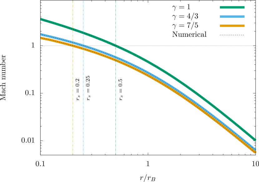
Figure 3: Comparison of the spherically symmetric numerical simulations performed with aztekas and the Bondi accretion solution corresponding to the adiabatic indices $\gamma=1,\,4/3,\,7/5$. The figure shows the Mach number versus radius for the three cases. Solid, coloured lines correspond to the Bondi solution while dashed, black lines correspond to the numerical results. The vertical dashed lines indicate the position of the sonic radius for each $\gamma$.

As a validation of the aztekas code in this work, we start by considering $\delta=0$, in which case spherical symmetry is recovered and the resulting accretion flow should coincide with the Bondi solution. In Figure 3 we show the results for the Mach number $\mathcal{M}=v/a$ as a function of the radial distance to the central object, as obtained from the three simulations with $\gamma=1,\,4/3,\,\text{and}\,\,7/5$ and compared to the corresponding analytic solutions. We find a very good agreement with the Bondi solution, with an error of less than 1% in the three cases (see Table 1). Further tests of aztekas against other analytic solutions and astrophysical problems can be found in Aguayo-Ortiz et al. (2018) and Tejeda & Aguayo-Ortiz (2019).

The treatment of the inner boundary is crucial for solving numerically the spherical accretion problem. One important point being whether the sonic surface is well resolved in the numerical domain or not. In the Bondi problem, the sonic surface appears at

$$r_{s}=\frac{5-3\gamma}{4}\,r_{B}.$$ (3.10)

As mentioned above, in all the simulations we placed the inner boundary at $\mathcal{R}_{\mathrm{acc}}=0.1\,r_{B}$ and, thus, the sonic surface is well resolved for all values of $\gamma$.

Note that we have not included the commonly used adiabatic index for a monoatomic gas $\gamma=5/3$, as in this case the sonic radius vanishes altogether. This makes a simulation which does not include artificial viscosity unstable to numerical fluctuations appearing at the inner boundary. We prefer not to include any such artificial effects so as to retain confidence in that the results obtained are a robust consequence of the physics being model.

3.3 Results

We now present the results for numerical simulations where the assumption of spherical symmetry for the infalling flow is relaxed, and parametrized through the density contrast $\delta$ as in equation (3.3).

To explore the relation between total infall and total outflow in the resulting steady state configurations, for each simulation we compute the mass accretion rate using equation (2.5). We apply this formula at each radial grid point and then take the average rate for all the domain. Likewise, we measure the injected and ejected mass rates across $\mathcal{R}$ using equations (2.9) and (2.10).

A summary of all of the simulations is shown in Table 1 where, for the various adiabatic indices and equatorial to polar density contrasts probed, we report the different accretion, injection and ejection rates, the ratio between ejection and injection, together with the location of the stagnation point and the maximum velocity attained by the outflowing material.

In order to validate these results, we performed a self-convergence test of the numerical solutions by increasing by a factor of 1.5 the resolution in both radial and angular coordinates. We obtained a second-order convergence as expected for a stationary shockless solution with an HRSC method (Lora-Clavijo & Guzmán, 2013).

$\gamma=1$ $\delta$ [%] $\frac{\dot{M}}{\dot{M}_{\mathrm{B}}}$ $\frac{\dot{M}_{\mathrm{in}}}{\dot{M}_{\mathrm{B}}}$ $\frac{\dot{M}_{\mathrm{ej}}}{\dot{M}_{\mathrm{B}}}$ $\frac{\dot{M}_{\mathrm{ej}}}{\dot{M}_{\mathrm{in}}}$ $\frac{\mathcal{S}}{r_{\mathrm{B}}}$ $\frac{v_{\mathrm{max}}}{v_{\mathrm{esc}}}$ $\frac{v_{\mathrm{max}}}{a}$ 0.0 0.99 0.99 0 0 – – – 0.1 0.99 1.95 0.94 0.48 5.10 0.130 0.057 1.0 1.02 4.18 3.16 0.75 3.35 0.373 0.164 10.0 1.05 9.99 8.94 0.89 2.55 1.182 0.520

$\gamma=4/3$

$\delta$ [%]	$\frac{\dot{M}}{\dot{M}_{\mathrm{B}}}$	$\frac{\dot{M}_{\mathrm{in}}}{\dot{M}_{\mathrm{B}}}$	$\frac{\dot{M}_{\mathrm{ej}}}{\dot{M}_{\mathrm{B}}}$	$\frac{\dot{M}_{\mathrm{ej}}}{\dot{M}_{\mathrm{in}}}$	$\frac{\mathcal{S}}{r_{\mathrm{B}}}$	$\frac{v_{\mathrm{max}}}{v_{\mathrm{esc}}}$	$\frac{v_{\mathrm{max}}}{a}$
0.0	1.00	1.00	0	0	–	–	–
0.1	1.00	2.55	1.55	0.61	4.50	0.130	0.057
1.0	1.01	5.60	4.59	0.82	3.29	0.376	0.166
10.0	1.04	15.44	14.40	0.93	2.16	1.186	0.522

$\gamma=7/5$ $\delta$ [%] $\frac{\dot{M}}{\dot{M}_{\mathrm{B}}}$ $\frac{\dot{M}_{\mathrm{in}}}{\dot{M}_{\mathrm{B}}}$ $\frac{\dot{M}_{\mathrm{ej}}}{\dot{M}_{\mathrm{B}}}$ $\frac{\dot{M}_{\mathrm{ej}}}{\dot{M}_{\mathrm{in}}}$ $\frac{\mathcal{S}}{r_{\mathrm{B}}}$ $\frac{v_{\mathrm{max}}}{v_{\mathrm{esc}}}$ $\frac{v_{\mathrm{max}}}{a}$ 0.0 0.99 0.99 0 0 – – – 0.1 1.00 2.76 1.76 0.63 4.34 0.130 0.057 1.0 1.01 6.23 5.22 0.83 3.17 0.376 0.166 10.0 1.04 17.41 16.37 0.94 2.05 1.188 0.523

Table 1: Simulations summary. In this table we give the accretion, injection and ejection rates in units of the corresponding Bondi rates (equation 2.7), ratio between ejection and injection, the position of the stagnation point along the vertical axis, as well as the ratio of the maximum ejection velocity to the local escape velocity and to the local speed of sound $a$.

In Figure 4, we show the resulting flow configurations for $\gamma=1$ and the four density contrasts. The figure shows the streamlines of the fluid together with isocontours of the density field. Figures 5 and 6 give the results for $\gamma=4/3$ and $\gamma=7/5$, respectively. In these figures, clear semicircles in the inner region of the numerical domain show the locations of the sonic surfaces in the Bondi solution, which can be seen to be resolved in all cases, as our domains start at $0.1\,r_{\mathrm{B}}$ in all cases.

\begin{overpic}[trim=0.0pt 65.24374pt 0.0pt 0.0pt,width=195.12767pt]{fig_4a.png} \end{overpic}

\begin{overpic}[trim=0.0pt 65.24374pt 0.0pt 0.0pt,width=195.12767pt]{fig_4b.png} \end{overpic}

\begin{overpic}[width=195.12767pt]{fig_4c.png} \end{overpic}

\begin{overpic}[width=195.12767pt]{fig_4d.png} \end{overpic}

Figure 4: Resulting steady state flow configurations for the numerical simulations for a fluid with equation of state $\gamma=1$ accreting onto a point mass. The different values of the density contrast $\delta$ used in each case are indicated on the top-left corner of each panel. The first panel gives the spherically symmetric case which, as expected, recovers the Bondi solution. As soon as $\delta\neq 0$ we see a qualitative change in the flow morphology, with even marginal departures from sphericity resulting in polar outflows. As the density contrast increases, the stagnation point reaches deeper into the accretion flow while the outflow region expands towards the equator. Streamlines are shown as black solid arrows. The grey scale gives the density profile, with some isodensity curves shown as black dashed lines (colour version online). The axes correspond to the usual cylindrical coordinates $R=r\,\sin\theta$, $z=r\,\cos\theta$. The clear semicircles at small radii identify the position of the Bondi sonic surface, in all cases located within the numerical domain, which begins at $0.1\,r_{\mathrm{B}}$.

\begin{overpic}[trim=0.0pt 65.24374pt 0.0pt 0.0pt,width=195.12767pt]{fig_5a.png} \end{overpic}

\begin{overpic}[trim=0.0pt 65.24374pt 0.0pt 0.0pt,width=195.12767pt]{fig_5b.png} \end{overpic}

\begin{overpic}[width=195.12767pt]{fig_5c.png} \end{overpic}

\begin{overpic}[width=195.12767pt]{fig_5d.png} \end{overpic}

Figure 5: Resulting steady state flow configurations for the numerical simulations with $\gamma=4/3$. The meaning of the different lines is the same as in Figure 4.

\begin{overpic}[trim=0.0pt 65.24374pt 0.0pt 0.0pt,width=195.12767pt]{fig_6a.png} \end{overpic}

\begin{overpic}[trim=0.0pt 65.24374pt 0.0pt 0.0pt,width=195.12767pt]{fig_6b.png} \end{overpic}

\begin{overpic}[width=195.12767pt]{fig_6c.png} \end{overpic}

\begin{overpic}[width=195.12767pt]{fig_6d.png} \end{overpic}

Figure 6: Resulting steady state flow configurations for the numerical simulations with $\gamma=7/5$. The meaning of the different lines is the same as in Figure 4.

In Figure 7 we show a close up of the inner region in the case of $\delta=10\%$. Here we show both the analytic value of the sonic radius (eq. 3.10), as well as the one extracted from our simulations. As can be seen, there is a very good agreement between both surfaces, even though the numerical ones do not correspond to a spherically symmetric accretion flow. This last illustrate the strong convergence of the solutions found towards the Bondi solution for small radii.

Moreover, we have analysed the distribution of the entropy and of the values of the Bernoulli constant among different streamlines. As expected for a perfect fluid in the absence of shocks, and due to our choice of the boundary conditions, the entropy remains constant throughout the entire numerical domain. On the other hand, for the Bernoulli constant, although it has a small variations from streamline to streamline, the mean value remains within 1 part in $10^{4}$ to the corresponding Bondi one, which agrees with the fact that $\dot{M}\approx\dot{M}_{\mathrm{B}}$.

\begin{overpic}[trim=0.0pt 65.24374pt 0.0pt 0.0pt,width=411.93767pt]{fig_7a.png} \end{overpic}

\begin{overpic}[trim=0.0pt 65.24374pt 0.0pt 0.0pt,width=411.93767pt]{fig_7b.png} \end{overpic}

\begin{overpic}[width=411.93767pt]{fig_7c.png} \end{overpic}

Figure 7: Close up of the inner region of the simulations with $\delta=10\%$ for the three values of $\gamma$. In the three panels we show the location of the sonic surface as extracted from the numerical simulations (dashed lines) together with the one corresponding to the Bondi solution (solid line).

4 Discussion

Based on the hydrodynamical numerical simulations presented in the previous section, we have explored the consequences of breaking spherical symmetry by imposing an axisymmetric, polar density contrast $\delta$ in the accretion flow. Naturally, when $\delta=0$ the spherically symmetric Bondi solution is recovered, as can be seen from Figure 3 and the top-left panel on Figures 4-6. However, as soon as there is a non-zero density contrast between the equatorial plane and the polar regions, the flow morphology changes qualitatively into an inflow/outflow configuration. The onset of even a quite marginal density contrast of $\delta=0.1\%$ results in the appearance of flow patterns highly resembling the analytic toy model discussed in Section 2 as well as the inflow/outflow configurations of the perturbative results of Hernandez et al. (2014) for an isothermal model.

As can be seen from the results reported in Table 1, as we take progressively larger values for the density contrast, the magnitude of the ejection velocities increases, and the position of the stagnation point moves towards smaller radii as the outflow region expands to occupy a larger fraction of the simulation domain. Note from Figures 4-6 that for $\delta=10\%$, the density contours appear slightly oblate, with the departure from spherical symmetry becoming more apparent. Moreover, for this same density contrast we obtain ejection velocities larger than the local escape velocity, while, at the same time, the ratio of mass ejection and mass injection rates reaches values as high as 94$\%$.

We have presented simulation results for three different values of the adiabatic index: $\gamma=1$, 4/3 and 7/5. Although we also explored intermediate values of $\gamma$, we do not include any further results, as they are all very similar and show a continuous progression between the cases presented. Indeed, we see that the three cases already considered are qualitatively very similar, as could have been anticipated from the qualitative similarities of the analytic solution of the highly simplified incompressible model presented in Section 2 and the slightly more realistic streamlines of the isothermal perturbative solutions of Hernandez et al. (2014). It is clear that breaking spherical symmetry with a polar density gradient in hydrodynamical accretion models leads to the same qualitative solutions with a morphology as shown in Figures 4-6.

In Figure 8 we show, for all of the simulations reported in this work, the ratio of the ejected and injected mass rates ($\dot{M_{\mathrm{ej}}}/\dot{M_{\mathrm{in}}}$) versus the injected mass rate in units of the corresponding Bondi value ($\dot{M_{\mathrm{in}}}/\dot{M_{\mathrm{B}}}$). The solid line represents the points where the injection and ejection of material are such that the total mass accretion rate equals the Bondi value, i.e.

$$\dot{M}=\dot{M}_{\rm in}-\dot{M}_{\rm ej}\equiv\dot{M}_{\mathrm{B}}.$$ (4.1)

From this figure we see that for $\dot{M_{\mathrm{in}}}/\dot{M_{\mathrm{B}}}=1$, the ejected mass is zero, while as $\dot{M_{\mathrm{in}}}/\dot{M_{\mathrm{B}}}$ increases, the ratio $\dot{M_{\mathrm{ej}}}/\dot{M_{\mathrm{in}}}$ tends to unity. It is remarkable that this dependency between injection and accretion holds quite accurately across the adiabatic index range sampled. Differences between $\dot{M}$ and $\dot{M_{\mathrm{B}}}$ remain beyond numerical resolution, but in all cases below a $5\%$ level. Thus, regardless of how large the injected mass rate is at the outer boundary, the central object only accretes at a maximum critical rate, closely corresponding to the Bondi mass accretion rate. This justifies our choice in equation (2.7) for the mass accretion rate of the analytic model of choked accretion.

The bipolar boundary density distribution adopted in equation (3.2) is not intended as a physical model corresponding to any specific situation, but rather as a convenient first order parametrization of departure from spherical symmetry. However, infall processes originating from accretion disc phenomena will quite probably be characterized by axisymmetric density profiles denser towards the equator than the poles. The details of the flow patterns resulting from particular situations will surely differ from the results presented here, although the clear convergence towards spherical accretion seen at small radii implies robustness in our conclusions with respect to this point. Indeed, the overall flow patterns obtained persist even when changing the particular parametrization used. Other similar density profiles were explored, obtaining consistent results, although very distinct boundary conditions may very well lead to substantially different solutions.

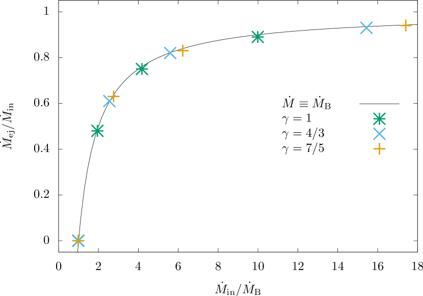
Figure 8: Ratio between the ejected and injected mass rates versus the injected mass rate in units of $\dot{M}_{\mathrm{B}}$ (see equation 2.7) for all of the simulations reported in this work. The solid line represents the case where the accretion rate onto the central object $\dot{M}$ is equal to the Bondi mass accretion rate.

Although the imposed geometry of the inflow boundary conditions necessarily leads to final configurations sharing the same symmetry, the resulting inflow/outflow morphology is by no means the only configuration sharing this symmetry, e.g. a pure infall configuration with oblate isodensity contours would have also satisfied the symmetry conditions alone. Further, the resulting limit on the accretion rate saturating close to the Bondi value is in no way evident simply from the assumption of a polar density gradient on the boundary conditions.

Let us explore now the viability of the choked accretion model to contribute towards the launching of a jet in different astrophysical settings. For this model we have neglected the effects of fluid rotation, which is a valid approximation just for the innermost part of an accretion disc where, through viscous transport mechanisms (e.g Balbus & Hawley, 1991), the disc material has lost most of its angular momentum. It is then natural to ask for the whole choked accretion machinery to fit within the inner walls of the disc. In other words, we require $\mathcal{S}$, the characteristic length scale of the choked accretion model, to be comparable to the physical size of this inner region.

Our simulation results show that $\mathcal{S}$ sinks deeper into the central region as we consider both larger density contrasts $\delta$ and larger adiabatic indices $\gamma$. We note, however, that for the parameters explored in this work $\mathcal{S}$ is always larger than the Bondi radius $r_{B}=\mathrm{G}M/a^{2}_{\infty}$. Assuming that this result holds in general, and considering an ideal gas composed of monoatomic hydrogen, we can write

$$a_{\infty}=\sqrt{\frac{\gamma\,k_{B}\,T_{\infty}}{m_{H}}}\simeq 3\times 10^{5}\left(\frac{T}{10^{3}\mathrm{K}}\right)^{1/2}\mathrm{cm}/\mathrm{s},$$ (4.2)

and, consequently, we have

$$\mathcal{S}\gtrsim 100\left(\frac{M}{M_{\odot}}\right)\left(\frac{T}{10^{3}\mathrm{K}}\right)^{-1}\mathrm{au},$$ (4.3)

or, in units of the gravitational radius $r_{g}=\mathrm{G}M/\mathrm{c}^{2}$

$$\mathcal{S}\gtrsim 5\times 10^{6}\left(\frac{T}{10^{6}\mathrm{K}}\right)^{-1}\,r_{g}.$$ (4.4)

These expressions should be considered as upper limits for $\mathcal{S}$. Additional physical ingredients that have been left out from this simple model can contribute to reduce this characteristic length scale. For example, we have neglected the necessary presence of radiation and magnetic fields in the system, both of which will result in an enhanced effective temperature, which will in turn result in smaller values of $\mathcal{S}$.

Let us consider the accretion discs behind X-ray binaries or AGNs. For these systems the inner border of the disc is expected to have a radius of the order of $1-10\,r_{g}$ and a temperature of around $T\sim 10^{6}\,\mathrm{K}$ (Czerny et al., 2003; Kaaret et al., 2017). From equation (4.4) we have $\mathcal{S}\gtrsim 10^{6}\,r_{g}$ and we can then conclude that these systems are too cold for choked accretion on its own to be responsible for the ejection.

On the other hand, for a Keplerian protoplanetary disc around a YSO we have inner radii in the order of $0.1-1.0\,\mathrm{au}$ and temperatures that can reach up to $10^{3}\,\mathrm{K}$ (Mori et al., 2019). In this case from equation (4.3) we obtain $\mathcal{S}\gtrsim 100\,\mathrm{au}$, which is two to three orders of magnitude larger than the presumed physical size of the system. Nevertheless, choked accretion might contribute to the ejection of molecular outflows associated to YSOs (Bachiller, 1996), as these outflows are driven by infalling matter and originate from regions farther than several $100\,\mathrm{au}$ from the central accretor.

Lastly, if we consider the central progenitors of long GRBs within the so-called collapsar scenario (Woosley & Bloom, 2006), we have again inner radii of the order of $1-10\,r_{g}$ but temperatures that can now reach up to $10^{11}\,\mathrm{K}$. From equation (4.4) for this temperature we obtain $\mathcal{S}\gtrsim 50\,r_{g}$, which is now within the expected order of magnitude for the mechanism presented to become relevant.

From these examples, it might seem that the length scale $\mathcal{S}$ on which the choked accretion mechanism operates is too large to contribute towards the ejection mechanism behind most astrophysical jets. It is important to keep in mind, however, that relaxing some of the simplifying assumptions behind the present model will necessarily lead to smaller values of $\mathcal{S}$. In addition to the already mentioned role played by radiation and magnetic fields, we have also seen a clear trend for diminishing values of $\mathcal{S}$ as the equatorial to polar density contrast increases. Hence, we can expect the applicability of the choked accretion mechanism to increase once larger density contrasts are considered.

In connection to the previous point, a non-zero angular momentum will naturally contribute to increase the density contrast between the material in the disc with respect to the polar regions (see e.g. Mendoza et al., 2009). We were not able to explore this regime in this work since from our numerical experiments we have found that taking larger values of $\delta$ or outer boundaries smaller than $r_{\mathrm{B}}$ lead to rather unstable, highly dynamic accretion flows that do not seem to relax to steady state configurations. We plan, however, to study both the effect of rotation and the dynamic regime resulting from steeper density gradients in future work.

There are additional physical processes, particularly non-adiabatic effects such as radiative cooling, heat transfer and shock formation, that can in principle modify our results. However, it is not clear a priori whether the inclusion of these effects will enhance or hamper the applicability of the choked accretion mechanism. We leave addressing these important points as the focus of future investigations, whereas the current simple model can be seen as presenting an underlying phenomenon which might be an important factor within a more general scheme.

5 Conclusions

Through simple analytic considerations for an idealized incompressible fluid, and axisymmetric numerical simulations for hydrodynamical accretion in a central Newtonian potential spanning a range of adiabatic indices, we have shown that large-scale, small amplitude departures from spherical symmetry, where the polar regions are under dense with respect to the equatorial plane, result in substantial qualitative and quantitative modifications in the resulting flow morphology.

Although the details depend on the particular choice of physical parameters, for the continuous bipolar boundary conditions explored, the resulting flow patterns are no longer the classical radial accretion ones, but have a consistent morphology comprising a central quasi-spherical accretion region, and an outer zone of equatorial infall and polar outflows.

We have seen that as the density contrast increases, a larger fraction of the mass injection rate is reversed and expelled along a bipolar outflow. Moreover, the maximum velocity attained by this ejected material can reach values larger than the local escape velocity.

As the accretion flow tends towards spherical symmetry at small radii, we find the interesting result that the total mass accretion rate is limited at a few percent above the Bondi value of the corresponding spherically symmetric case. Thus, hydrodynamical accretion towards central objects appears to choke at a maximum value, with any extra input material fuelling the bipolar outflow.

In conclusion, we have presented compelling evidence for the existence of a choked accretion phenomenon in hydrodynamical flows onto gravitating objects. Furthermore, we have shown that choked accretion works as a hydrodynamical mechanism for ejecting axisymmetric outflows, thus constituting a transition bridge between purely radial accretion flows and jet-generating systems.

References

- Aguayo-Ortiz et al. (2018) Aguayo-Ortiz A., Mendoza S., Olvera D., 2018, PLoS ONE, 13, e0195494
- Awe et al. (2011) Awe T. J., Adams C. S., Davis J. S., Hanna D. S., Hsu S. C., Cassibry J. T., 2011, Physics of Plasmas, 18, 072705
- Bachiller (1996) Bachiller R., 1996, Ann. Rev. Ast. & Ast., 34, 111
- Balbus & Hawley (1991) Balbus S. A., Hawley J. F., 1991, Astrophysical Journal, 376, 214
- Blandford (1976) Blandford R. D., 1976, Monthly Notices of the Royal Astronomical Society, 176, 465
- Blandford & Payne (1982) Blandford R. D., Payne D. G., 1982, Monthly Notices of the Royal Astronomical Society, 199, 883
- Blandford & Rees (1974) Blandford R. D., Rees M. J., 1974, Monthly Notices of the Royal Astronomical Society, 169, 395
- Blandford & Znajek (1977) Blandford R. D., Znajek R. L., 1977, Monthly Notices of the Royal Astronomical Society, 179, 433
- Bondi (1952) Bondi H., 1952, Monthly Notices of the Royal Astronomical Society, 112, 195+
- Canto & Rodriguez (1980) Canto J., Rodriguez L. F., 1980, Astrophysical Journal, 239, 982
- Casse & Keppens (2002) Casse F., Keppens R., 2002, ApJ, 581, 988
- Currie (2003) Currie I. G., 2003, Fundamental mechanics of fluids, 3rd edn. New York: Marcel Dekker
- Czerny et al. (2003) Czerny B., Nikołajuk M., Różańska A., Dumont A. M., Loska Z., Zycki P. T., 2003, Astronomy and Astrophysics, 412, 317
- Del Zanna et al. (1998) Del Zanna L., Velli M., Londrillo P., 1998, Astronomy and Astrophysics, 330, L13
- Harten et al. (1983) Harten A., Lax P. D., Leer B., 1983, SIAM Review, 25
- Hawley et al. (2015) Hawley J. F., Fendt C., Hardcastle M., Nokhrina E., Tchekhovskoy A., 2015, Space Science Reviews, 191, 441
- Hernandez et al. (2014) Hernandez X., Rendón P. L., Rodríguez-Mota R. G., Capella A., 2014, Revista Mexicana de Astronomía y Astrofísica, 50, 23
- Jafari (2019) Jafari A., 2019, arXiv e-prints, p. arXiv:1904.09677
- Kaaret et al. (2017) Kaaret P., Feng H., Roberts T. P., 2017, Ann. Rev. Ast. & Ast., 55, 303
- Lery et al. (2002) Lery T., Henriksen R. N., Fiege J. D., Ray T. P., Frank A., Bacciotti F., 2002, Astronomy and Astrophysics, 387, 187
- Liska et al. (2019) Liska M., Tchekhovskoy A., Ingram A., van der Klis M., 2019, MNRAS, 487, 550
- Lora-Clavijo & Guzmán (2013) Lora-Clavijo F. D., Guzmán F. S., 2013, Monthly Notices of the Royal Astronomical Society, 429, 3144
- Lovelace (1976) Lovelace R. V. E., 1976, Nature, 262, 649
- Mendoza et al. (2009) Mendoza S., Tejeda E., Nagel E., 2009, Monthly Notices of the Royal Astronomical Society, 393, 579
- Michel (1972) Michel F. C., 1972, Astrophysics and Space Science, 15, 153
- Mirabel & Rodríguez (1994) Mirabel I. F., Rodríguez L. F., 1994, Nature, 371, 46
- Mori et al. (2019) Mori S., Bai X.-N., Okuzumi S., 2019, ApJ, 872, 98
- Olvera & Mendoza (2008) Olvera D., Mendoza S., 2008, in Oscoz A., Mediavilla E., Serra-Ricart M., eds, EAS Publications Series Vol. 30 of EAS Publications Series, A GPL Relativistic Hydrodynamical Code. pp 399–400
- Petrich et al. (1988) Petrich L. I., Shapiro S. L., Teukolsky S. A., 1988, Physical Review Letters, 60, 1781
- Pudritz et al. (2007) Pudritz R. E., Ouyed R., Fendt C., Brandenburg A., 2007, Protostars and Planets V, pp 277–294
- Qian et al. (2018) Qian Q., Fendt C., Vourellis C., 2018, ApJ, 859, 28
- Romero et al. (2017) Romero G. E., Boettcher M., Markoff S., Tavecchio F., 2017, Space Science Reviews, 207, 5
- Semenov et al. (2004) Semenov V., Dyadechkin S., Punsly B., 2004, Science, 305, 978
- Shakura & Sunyaev (1973) Shakura N. I., Sunyaev R. A., 1973, Astronomy and Astrophysics, 24, 337
- Sheikhnezami & Fendt (2018) Sheikhnezami S., Fendt C., 2018, ApJ, 861, 11
- Shu & Osher (1988) Shu C.-W., Osher S., 1988, Journal of Computational Physics, 77, 439
- Tchekhovskoy (2015) Tchekhovskoy A., 2015, 414
- Tejeda (2018) Tejeda E., 2018, Revista Mexicana de Astronomía y Astrofísica, 54, 171
- Tejeda & Aguayo-Ortiz (2019) Tejeda E., Aguayo-Ortiz A., 2019, MNRAS, 487, 3607
- Tejeda et al. (2019) Tejeda E., Aguayo-Ortiz A., Hernandez X., 2019, arXiv e-prints, p. arXiv:1909.01527
- Velli (1994) Velli M., 1994, ApJL, 432, L55
- Woosley & Bloom (2006) Woosley S. E., Bloom J. S., 2006, Annual Review of Astronomy and Astrophysics, 44, 507