Simple explanation of strong suppression of fermionic EFT operators & custodial symmetry breaking

Abstract:

The present approach relies on the SM chiral symmetry breaking pattern $SU(2)_{L}\otimes SU(2)_{R}\to SU(2)_{L+R}$, with the EW Goldstone bosons given in a non-linear realization and the Higgs boson described by an EW singlet field. In addition, we assume the presence of new physics heavy states around the TeV scale that do not couple to the SM fermions, only to the SM bosonic sector. However, the mixing between gauge bosons and BSM resonances induces a small indirect interaction between the BSM sector and the SM fermions. This leads to an important suppression of the fermionic operators in the low-energy EW effective theory (bilinear and four-fermion operators) in comparison with the purely bosonic ones. This naturally explains the strong experimental bounds on fermionic operators and why these resonances could not be yet detected: even if energies of the order of the TeV can be reached in present and future accelerators, their production from initial SM fermions yields a very small cross section because of this suppression mechanism. On the other hand, they can leave an imprint in SM boson measurements accessible to future experimental runs (e.g., the oblique $S$ and $T$ parameters). Finally, we compare our results with constraints from collider data.

1 Introduction

The search for physics beyond the Standard Model (BSM) has put very stringent limits on the masses of spin 1 particles coupling to Standard Model (SM) fermions [2, 3, 4]. These bounds are obtained using operators with canonical dimension 6 such as Fermi-like operators, this is, four-fermion contact interactions. The inverse mass scale parameter in the Lagrangian density is often taken to be the mass of such BSM field. The problem with this approach is that such field may not couple directly to the SM fermions, which might found additional suppression due to the need of a mediator between these fields. If one relies on effective Chiral Lagrangians to recover the SM operators and regard the BSM spin 1 fields as resonances that do not couple directly to the SM fermions, a natural suppression to observables involving fermions comes about due to a need for additional exchange of SM gauge bosons. In this work we show that these rather stringent experimental limits may not necessarily imply such restrictive bounds on the masses of the resonances, by means of a somewhat naive estimation of such masses. We also obtain a more elaborate estimation of the masses of spin 1 resonances using experimental bounds on the oblique $S$ and $T$ parameters [5, 6, 7, 8].

Considering the electroweak sector of the Standard Model (SM) to be described by an effective theory of a more fundamental strongly-coupled theory, where its scalar sector symmetry group can be generalized to that of the Electroweak Effective Theory (EWET), the Electroweak Chiral Symmetry group $G=SU(2)_{L}\otimes SU(2)_{R}$. Relying on this symmetry and without adding more fields than those of the SM, an effective field theory at low energies of such strongly-coupled theory can be developed to describe the interactions of these fields. The procedure is then completely analogous to that of Chiral Perturbation Theory ($\chi$PT) [9, 10, 11]: The Electroweak Chiral Symmetry gets spontaneously broken to the custodial symmetry, $H=SU(2)_{L+R}$, which generates three Goldstone bosons. Afterwards and in order to recover the SM interactions, the third generator of $SU(2)_{R}$ is identified as the SM hypercharge field, while the other two are regarded as non-propagating external currents. This gives an explicit symmetry breaking to $SU(2)_{L}\otimes U(1)_{Y}$. It is worth to notice that the physical Higgs field is a scalar under the whole Electroweak Chiral Symmetry group. Another key ingredient of the theory is the non-linear realization of the EW Goldstone bosons. This leads to a theory resembling $\chi$PT and that can be developed in an analogous way and expanded in chiral powers. With the chiral counting given in ref. [12, 13], the SM operators will be given by the lowest chiral dimension Lagrangian density $\hat{d}=2$.

Just as $\chi$PT can be naturally extended to include meson resonances [14, 15], so can the EWET [12, 13] be extended to include resonances. From the resonances Lagrangian the equations of motion (EoM) are obtained and then substituted to obtain the low-energy contribution to the couplings of the EWET theory Lagrangian density of chiral dimension $\hat{d}=4$. This has been done previously in [12]. However, the novelty in our calculation is that we take into account the NLO contribution to the EoM of the resonances, obtaining new effects such as, eg, a non-vanishing contribution to the oblique $T$ parameter. Since LEP [4] gives the most precise data for the $S$ and $T$ parameters, we use this data set to obtain bounds on the polar-vector mass and in the axial- to polar-vector resonance masses ratio.

2 Electroweak Effective Theory

The Electroweak Effective Theory is based in the spontaneous symmetry breaking of the Electroweak Chiral Symmetry $G=SU(2)_{L}\otimes SU(2)_{R}$ to the custodial symmetry $H=SU(2)_{L+R}$. If the four fundamental scalar fields of the SM are collected in a $2\times 2$ matrix [12]

$$\Sigma=\left(\begin{array}[]{cc}{\Phi^{0}}^{*}&\Phi^{+}\\ -\Phi^{-}&\Phi^{0}\end{array}\right),$$ (1)

the Lagrangian of these fields is given by

$$\mathcal{L}(\Phi)=\frac{1}{2}\left\langle\left(D^{\mu}\Sigma\right)^{\dagger}D_{\mu}\Sigma\right\rangle-\frac{\lambda}{16}\left(\left\langle\Sigma^{\dagger}\Sigma\right\rangle-v^{2}\right)^{2},$$ (2)

where

$$D_{\mu}\Sigma=\partial_{\mu}\Sigma+ig\frac{\overrightarrow{\sigma}}{2}\cdot\overrightarrow{W}_{\mu}\Sigma-ig^{\prime}\Sigma\frac{\overrightarrow{\sigma}}{2}\cdot\overrightarrow{B}_{\mu},$$ (3)

$v=246$ GeV is the EW vacuum expectation value, $g$ and $g^{\prime}$ the gauge group couplings and $\sigma_{i}$ the Pauli matrices. Instead of representing the scalar sector of the SM in cartesian components (linear representation), it is given in a polar representation (non-linear representation) as follows

$$\Sigma(x)=\frac{1}{\sqrt{2}}\left[v+h(x)\right]U(\varphi(x)),$$ (4)

where $h$ is the physical Brout-Englert-Higgs (BEH) field and $U$ transforms under $G$ as

$$U(\varphi)=\exp\left\{i\overrightarrow{\sigma}\cdot\frac{\overrightarrow{\varphi}}{v}\right\}\xrightarrow{\hskip 4.30554ptG\hskip 4.30554pt}g_{L}U(\varphi)g_{R}^{\dagger}\hskip 86.11084ptg_{L,R}\in SU(2)_{L,R}.$$ (5)

This means that $\mathcal{L}(\Phi)$ can be written as

$$\mathcal{L}(\Phi)=\frac{v^{2}}{4}\left\langle\left(D^{\mu}U\right)^{\dagger}D_{\mu}U\right\rangle+\frac{1}{2}\left(\partial_{\mu}h\hskip 2.15277pt\partial^{\mu}h\right)-V(h).$$ (6)

In the unitary gauge $U=1$, and one recovers the SM values for the masses of the gauge bosons in terms of the vev, $g$ and $g^{\prime}$. This procedure is, however, equivalent to selecting a definite non-linear representation of the coset $G/H$ coordinates $(u_{L}(\varphi),u_{R}(\varphi))\to(U(\varphi),1)$, where $U(\varphi)=u_{L}(\varphi)u_{R}^{\dagger}(\varphi)$, and the general coordinates transform as [16, 17]

$$u_{\chi}(\varphi)\xrightarrow{\hskip 4.30554ptG\hskip 4.30554pt}g_{\chi}u_{\chi}(\varphi)g_{h}^{\dagger}(\varphi,g),$$ (7)

for $\chi=R,L$, where $g=(g_{L},g_{R})\in G$. A more convenient representation of the Goldstone fields for the extension of the model (when the resonances are included), is obtained for $u(\varphi)=u_{L}(\varphi)=u_{R}^{\dagger}(\varphi)$, where

$$u(\varphi)=\exp\left\{i\overrightarrow{\sigma}\cdot\frac{\overrightarrow{\varphi}}{2v}\right\}.$$ (8)

Tensors transforming as triplets under the vector subgroup $H$, $R\to g_{h}Rg_{h}^{\dagger}$, have covariant derivatives

$$\nabla_{\mu}R=\partial_{\mu}R+\left[\Gamma_{\mu},R\right]\hskip 15.0694pt\xrightarrow{\hskip 4.30554ptG\hskip 4.30554pt}\hskip 15.0694ptg_{h}\nabla_{\mu}Rg_{h}^{\dagger},$$ (9)

where the connection is

$$\Gamma_{\mu}=\frac{1}{2}\left(\Gamma^{L}_{\mu}+\Gamma^{R}_{\mu}\right),\hskip 17.22217pt\Gamma^{\chi}_{\mu}=u^{\dagger}_{\chi}(\varphi)\left(\partial_{\mu}-i\hat{\chi}_{\mu}\right)u_{\chi}(\varphi)$$ (10)

being $\hat{\chi}_{\mu}=\hat{W}_{\mu},\hat{B}_{\mu}$ for $\chi=L,R$ respectively. Since the physical Higgs boson transforms as a scalar under the whole symmetry of the Lagrangian density, there is no restriction as to how many of such fields can be considered in the Lagrangian density. Therefore, every operator in the Lagrangian density must be multiplied by a power series in $x=h/v$. Thus, the scalar sector Lagrangian density, $\mathcal{L}(\Phi)$, is expressed as

$$\mathcal{L}(\Phi)=\frac{v^{2}}{4}\mathcal{F}_{u}\left\langle u_{\mu}u^{\mu}\right\rangle+\frac{1}{2}\left(\partial_{\mu}h\hskip 2.15277pt\partial^{\mu}h\right)-V,$$ (11)

where

$$u_{\mu}=u_{\mu}^{\dagger}=i\left(\Gamma^{R}_{\mu}-\Gamma^{L}_{\mu}\right)=i\left[u(\partial_{\mu}-i\hat{B}_{\mu})u^{\dagger}-u^{\dagger}(\partial_{\mu}-i\hat{W}_{\mu})u\right],$$ (12)

being $\mathcal{F}_{u}$ and $V$ power series of $x$ whose lowest order term are $1$ and the Higgs mass term respectively. The part concerning the gauge bosons and their interactions are given by the familiar Yang-Mills Lagrangian.

$$\mathcal{L}_{\textrm{\scriptsize YM}}=-\frac{1}{2g^{2}}\hat{W}_{\mu\nu}\hat{W}^{\mu\nu}-\frac{1}{2g^{\prime 2}}\hat{B}_{\mu\nu}\hat{B}^{\mu\nu},$$ (13)

where the field strength tensors are given by

$$\hat{W}_{\mu\nu} = \partial_{\mu}\hat{W}_{\nu}-\partial_{\nu}\hat{W}_{\mu}-i\left[\hat{W}_{\mu},\hat{W}_{\nu}\right],$$

$$\hat{B}_{\mu\nu} = \partial_{\mu}\hat{B}_{\nu}-\partial_{\nu}\hat{B}_{\mu}-i\left[\hat{B}_{\mu},\hat{B}_{\nu}\right].$$ (14)

Here, $\hat{W}_{\mu}=-gW^{i}_{\mu}\frac{\sigma^{i}}{2}$ where $\sigma^{i}$ are the $SU(2)_{L}$ Pauli matrices and similarly $\hat{B}_{\mu}=-g^{\prime}B^{i}_{\mu}\frac{\sigma^{i}}{2}$ for the $SU(2)_{R}$ group. The fermionic sector of the EWET is given by the Lagrangian density

$$\mathcal{L}_{\psi}=i\overline{\psi}\not{D}\psi-v^{2}\langle J_{S}\rangle,$$ (15)

where $J_{S}=J_{Y}+J_{Y}^{\dagger}$, being $J_{Y}=(1/v)\overline{\xi}_{L}\mathcal{Y}\xi_{R}$ and $\mathcal{Y}$ a power series in $x$ whose order zero term gives the SM Yukawa couplings. Here, the covariant derivative is given by the following expression

$$D_{\mu}^{\chi}\psi_{\chi}=\left(\partial_{\mu}-i\hat{\chi}_{\mu}-i\hat{X}_{\mu}\frac{\mathfrak{B}-\mathfrak{L}}{2}\right)\psi_{\chi},$$ (16)

where $\hat{\chi}_{\mu}=\hat{B}_{\mu},\hat{W}_{\mu}$ for $\chi=R,L$, being $\psi_{R/L}=\frac{1}{2}(1\pm\gamma_{5})\psi$ the chirality projection of the Dirac spinor and the $\mathfrak{B}$ and $\mathfrak{L}$ operators that act on the fermion fields, whose eigenvalues are the barion and lepton numbers respectively. The chiral projections of the fermion fields transform under $G$ as

$$\psi_{\chi}\to g_{\chi}\psi_{\chi}.$$ (17)

A spinor transforming under the custodial symmetry group $SU(2)_{L+R}$ can be obtained multiplying the left (right) Weyl spinor by $u_{L/R}^{\dagger}$

$$\xi_{\chi}=u_{\chi}^{\dagger}\psi_{\chi},\hskip 25.83325pt\overline{\xi}_{\chi}=\overline{\psi}_{\chi}u_{\chi},$$ (18)

so that one gets a new spinor which transform under $G$ as $\xi_{\chi}\to g_{h}\xi_{\chi}$, with $g_{h}\in SU(2)_{L+R}$. To recover the Standard Model, the coupling between the $\hat{X}$ field and the SM fermions given in eq. (16) must be such that $\hat{X}$ is the SM hypercharge field,

$$\hat{X}_{\mu}=-g^{\prime}B_{\mu}.$$ (19)

For future reference, we define the left and right fermion currents as

$$\left(J^{\ell}_{\mu}\right)_{mn} =\frac{1}{2}{\overline{\xi}_{n}\gamma_{\mu}(1-\gamma_{5})\xi_{m}},$$ (20a)

$$\left(J^{r}_{\mu}\right)_{mn} =\frac{1}{2}{\overline{\xi}_{n}\gamma_{\mu}(1+\gamma_{5})\xi_{m}},$$ (20b)

where $m$ and $n$ are flavor indices transforming under $SU(2)_{L+R}$.

3 Equations of motion for SM bosons

The equations of motion for the Goldstone bosons are given by the following expressions

$$\nabla_{\mu}u^{\mu}=-u^{\mu}\partial_{\mu}\left(\frac{h}{v}\right)\frac{\mathcal{F}_{u}^{\prime}}{\mathcal{F}_{u}}-\frac{2}{\mathcal{F}_{u}}J_{P}+\frac{1}{\mathcal{F}_{u}}\langle J_{P}\rangle,$$ (21)

where $J_{P}=i(J_{Y}-J_{Y}^{\dagger})$ and the prime on the functions of the BEH boson means that it is derived with respect to $x=h/v$. For the BEH field we have

$$\Box\left(h/v\right)=\frac{1}{4}\mathcal{F}_{u}^{\prime}\langle u_{\mu}u^{\mu}\rangle-V^{\prime}-\langle J_{S}^{\prime}\rangle.$$ (22)

For the gauge boson fields we find

$$D^{\nu}\hat{W}_{\nu\mu,i} =\frac{(gv)^{2}}{4}\mathcal{F}_{u}\langle u_{\mu}\sigma_{i}^{L}\rangle+\frac{g^{2}}{2}\langle\xi^{\alpha}_{L}\overline{\xi}^{\beta}_{L}\gamma_{\mu}^{\beta\alpha}\sigma_{i}^{L}\rangle,$$ (23a)

$$D^{\nu}\hat{B}_{\nu\mu,i} =-\frac{(g^{\prime}v)^{2}}{4}\mathcal{F}_{u}\langle u_{\mu}\sigma_{i}^{R}\rangle+\frac{g^{\prime 2}}{2}\langle\xi^{\alpha}_{R}\overline{\xi}^{\beta}_{R}\gamma_{\mu}^{\beta\alpha}\sigma_{i}^{R}\rangle-(g^{\prime})^{2}\overline{\psi}\gamma_{\mu}\frac{\mathfrak{B}-\mathfrak{L}}{2}\delta_{3,i}\psi,$$ (23b)

where $\beta$ and $\alpha$ are spinor indices, $\delta_{3,i}$ is the Kronecker delta, $\sigma_{i}^{\chi}=u_{\chi}^{\dagger}\sigma_{i}u_{\chi}$ for $\chi=R,L$ and $D^{\nu}\hat{X}_{\nu\mu,i}=\langle D^{\nu}\hat{X}_{\nu\mu}\sigma_{i}\rangle$. Nevertheless, it must be noticed that the only physical equation of motion in eqs. (23b) is that of $\hat{B}^{3}$. When the $B^{1}$ and $B^{2}$ fields vanish, this gives

$$\partial^{\nu}B_{\nu\mu}=-\frac{(g^{\prime}v)^{2}}{4}\mathcal{F}_{u}\left(u_{L}u_{\mu}u_{L}^{\dagger}\right)_{3}+\frac{g^{\prime 2}}{2}\left(\psi^{\alpha}_{L}\overline{\psi}^{\beta}_{L}\gamma_{\mu}^{\beta\alpha}\right)_{3}-\frac{(g^{\prime}v)^{2}}{2}{J_{X}}_{\mu},$$ (24)

where $B_{\mu\nu}=\partial_{\mu}\hat{B}^{3}_{\nu}-\partial_{\nu}\hat{B}^{3}_{\mu}$ and $J_{X}^{\mu}=\overline{\xi}_{m}\gamma^{\mu}\frac{\mathfrak{B}-\mathfrak{L}}{v^{2}}\xi_{m}$, being $m$ the $SU(2)_{L+R}$ index of the spinors and a sum over repeated indices is implied, meaning that the current $J_{X}$ behaves as a scalar under the chiral group. It must be noticed that any contribution of the fields $\hat{B}^{1}$ and $\hat{B}^{2}$ must be neglected in the calculation of vertex functions since they are regarded as external currents, instead of fundamental fields and, therefore, are to be considered to vanish. However, these fields are needed in order to use relations allowing us to express eqs. (23) as operators transforming under the residual custodial symmetry. Thus, the covariant derivatives in eq.(23) can be expressed as

$$D^{\nu}\hat{W}_{\nu\mu,i} =\langle\nabla^{\nu}f^{L}_{\nu\mu}\sigma_{i}^{L}\rangle-\frac{i}{2}\langle\left[f^{L}_{\nu\mu},u^{\nu}\right]\sigma_{i}^{L}\rangle,$$ (25a)

$$D^{\nu}\hat{B}_{\nu\mu,i} =\langle\nabla^{\nu}f^{R}_{\nu\mu}\sigma_{i}^{R}\rangle+\frac{i}{2}\langle\left[f^{R}_{\nu\mu},u^{\nu}\right]\sigma_{i}^{R}\rangle,$$ (25b)

where $f^{L/R}_{\mu\nu}=\frac{1}{2}({f_{+}}_{\mu\nu}\pm{f_{-}}_{\mu\nu})$, where

$$f^{\mu\nu}_{\pm}=u^{\dagger}\hat{W}^{\mu\nu}u\pm u\hskip 2.15277pt\hat{B}^{\mu\nu}u^{\dagger}.$$ (26)

Putting together eqs. (23a), (23b) for $i=3$ and (25) we find the following relations

$$\nabla^{\nu}f^{L}_{\mu\nu}= \frac{i}{2}\left[f^{L}_{\mu\nu},u^{\nu}\right]-\frac{(gv)^{2}}{4}\mathcal{F}_{u}u_{\mu}-\frac{g^{2}}{2}\xi^{\alpha}_{L}\overline{\xi}^{\beta}_{L}\gamma_{\mu}^{\beta\alpha}+\frac{g^{2}}{4}\langle\xi^{\alpha}_{L}\overline{\xi}^{\beta}_{L}\gamma_{\mu}^{\beta\alpha}\rangle,$$ (27a)

$$\nabla^{\nu}f^{R}_{\mu\nu}= \left\langle\left(-\frac{i}{2}\left[f^{R}_{\mu\nu},u^{\nu}\right]+\frac{(g^{\prime}v)^{2}}{4}\mathcal{F}_{u}u_{\mu}-\frac{\left(g^{\prime}\right)^{2}}{2}\xi^{\alpha}_{R}\overline{\xi}^{\beta}_{R}\gamma_{\mu}^{\beta\alpha}\right)\sigma_{3}^{R}\right\rangle\frac{\sigma_{3}^{R}}{2}$$

$$+\frac{(g^{\prime}v)^{2}}{2}{J_{X}}_{\mu}\frac{\sigma_{3}^{R}}{2}+\widetilde{\nabla^{\nu}f^{R}_{\mu\nu}},$$ (27b)

where $\widetilde{\nabla^{\nu}f^{R}_{\mu\nu}}=\sum_{i=1,2}\left\langle{\nabla^{\nu}f^{R}_{\mu\nu}}\sigma_{i}^{R}\right\rangle\frac{\sigma_{i}^{R}}{2}$. One of the main advantages of formulating the SM using the chiral symmetry is that all the SM is given by the most general Lagrangian with chiral dimension $\hat{d}=2$, meaning that NLO operators will encode only BSM interactions.

4 Resonance contribution to low energy constants

4.1 Equations of motion of spin 1 resonances

In an analogous way to the extension of $\chi$PT which incorporates the meson resonances as active degrees of freedom [14, 15], one can include resonances to obtain their contribution to the couplings of the $\mathcal{O}(p^{4})$ chiral Lagrangian operators [12, 13]. Thus, one must obtain the equations of motion of the resonances and substitute the expressions for the classical fields in the Lagrangian for these resonances. In the antisymetric formalism [15], such Lagrangian for spin = 1 resonances is

$$\mathcal{L}_{R}=-\frac{1}{2}\left\langle\nabla^{\lambda}R_{\lambda\mu}\nabla_{\sigma}R^{\sigma\mu}-\frac{1}{2}M_{R}^{2}R_{\mu\nu}R^{\mu\nu}\right\rangle+\left\langle R_{\mu\nu}\chi^{\mu\nu}_{R}\right\rangle\hskip 21.52771pt\left(R=V,A\right),$$ (28)

The definitions of $\chi_{R}^{\mu\nu}$ for $R=V,A$ are given as follows [12, 13]

$$\chi_{V}^{\mu\nu} =\frac{F_{V}}{2\sqrt{2}}f_{+}^{\mu\nu}+\frac{\widetilde{F}_{V}}{2\sqrt{2}}f_{-}^{\mu\nu}+i\frac{G_{V}}{2\sqrt{2}}\left[u^{\mu},u^{\nu}\right]+\frac{\widetilde{\lambda}_{1}^{hV}}{\sqrt{2}}\left[\left(\partial^{\mu}h\right)u^{\nu}-\left(\partial^{\nu}h\right)u^{\mu}\right],$$ (29a)

$$\chi_{A}^{\mu\nu} =\frac{\widetilde{F}_{A}}{2\sqrt{2}}f_{+}^{\mu\nu}+\frac{F_{A}}{2\sqrt{2}}f_{-}^{\mu\nu}+i\frac{\widetilde{G}_{A}}{2\sqrt{2}}\left[u^{\mu},u^{\nu}\right]+\frac{\lambda_{1}^{hA}}{\sqrt{2}}\left[\left(\partial^{\mu}h\right)u^{\nu}-\left(\partial^{\nu}h\right)u^{\mu}\right],$$ (29b)

where the couplings with tilde mean that the corresponding operator in the Lagrangian 28 do not conserve parity. Thus, the axial-vector resonance contribution to the EWET Lagrangian couplings can be obtained from the polar-vector ones by making the substitutions $F_{V}\to\widetilde{F}_{A}$, $\widetilde{F}_{V}\to F_{A}$, $\widetilde{\lambda}^{hV}_{1}\to\lambda^{hA}_{1}$ and $G_{V}\to\widetilde{G}_{A}$. Notice that all coupling constants have canonic dimension 1 except for $\widetilde{\lambda}_{1}^{hV}$ and $\lambda_{1}^{hA}$, which are canonically dimensionless. The equations of motion for the resonances are given by the following expression [14]

$$\nabla^{\mu}\nabla_{\sigma}R^{\sigma\nu}-\nabla^{\nu}\nabla_{\sigma}R^{\sigma\mu}+M_{R}^{2}R^{\mu\nu}=-2\chi^{\mu\nu}_{R}$$ (30)

with which the classical field expressions for the resonance fields are given by

$$R^{\mu\nu}_{class}=-\frac{2}{M_{R}^{2}}\chi^{\mu\nu}+\frac{2}{M_{R}^{2}}\left[\nabla^{\nu}\nabla_{\sigma}\left(\frac{\chi^{\mu\sigma}_{R}}{M_{R}^{2}}\right)-\nabla^{\mu}\nabla_{\sigma}\left(\frac{\chi^{\nu\sigma}_{R}}{M_{R}^{2}}\right)\right]+\mathcal{O}\left(p^{6}\right)$$ (31)

Substituting the previous expression in the Lagrangian for the resonance field gives the contribution to the EWET couplings of the Lagrangian

$$\mathcal{L}_{R}(R_{class})=-\frac{1}{M_{\hat{R}}^{2}}\langle\chi^{\mu\nu}_{R}\chi_{\mu\nu,R}\rangle-2\left\langle\nabla_{\nu}\left(\frac{\chi^{\mu\nu}_{R}}{M_{R}^{2}}\right)\nabla^{\sigma}\left(\frac{\chi_{\mu\sigma,R}}{M_{R}^{2}}\right)\right\rangle+\mathcal{O}(p^{8}),$$ (32)

where the term with the covariant derivatives is the novel contribution to the EoM, which considering the gauge and Goldstone fields EoM gives, among other effects, a custodial symmetry breaking term contributing to the oblique $T$ parameter [1, 12, 18].

5 Phenomenology

Using the equations of motion for the Goldstone and gauge bosons in $\mathcal{L}_{R}(R_{class})$, the contribution to the couplings of the EWET Lagrangian is obtained by making a comparison with the full $\mathcal{O}(p^{4})$ basis given in reference [12, 13]. Thus, the four-fermion contact interaction given in the phenomenological Lagrangian in references [2, 3, 4]

$$\mathcal{L}_{EWET}\supset\mathcal{L}_{qq}=\frac{2\pi}{\Lambda^{2}}\left(\eta_{\ell\ell}J^{\ell}_{\mu}J^{\ell,\mu}+\eta_{rr}J^{r}_{\mu}J^{r,\mu}+2\eta_{r\ell}J^{r}_{\mu}J^{\ell,\mu}\right),$$ (33)

can be expressed as a linear combination of the terms in $\mathcal{L}_{EWET}$. The most stringent experimental bound on the BSM scale is found for $\eta_{\ell\ell}=\eta_{rr}=\eta_{r\ell}=-1$, which is $\Lambda\gtrsim 20$ TeV. This parameter $\Lambda$ is commonly taken to be the compositeness scale or the mass of the resonance, however since in our model the resonances do not couple directly to the SM fermions, the former statement is not true. Comparing this with the contribution from the spin 1 resonances and after using the Weinberg sum rules [19] we get

$$\frac{2\pi}{\Lambda^{2}}=\frac{4m_{Z}^{4}-8m_{Z}^{2}m_{W}^{2}+7m_{W}^{4}}{24v^{2}M_{V}^{4}}\,\,\frac{r^{3}+1}{r^{2}(r-1)},$$ (34)

where $r=M_{A}^{2}/M_{V}^{2}$. Some bounds on the vector resonance mass and the ratio $r$ are given in Table 1, where we take $\Lambda\geq$20 TeV. These are, however, not to be regarded as precise predictions of the model, since this naive approach gives an estimation that does not consider correlation among the $\eta_{ij}$ parameters in eq. (33).

$r=M_{A}^{2}/M_{V}^{2}$	lower bound for $M_{V}$
$1+10^{-3}$	$1.9$ TeV
$1.1$	$0.6$ TeV
$2$	$0.3$ TeV
$\infty$	$0.3$ TeV

Table 1: Bounds for $M_{V}$ as a function of the ratio $r$ using the experimental bound $\Lambda\gtrsim 20$ TeV.

To give a more elaborate estimation of the vector resonance mass as a function of the ratio of spin 1 resonance masses we make use of the contributions to the $S$ and $T$ oblique parameters. The $S$ and $T$ parameters can be given as functions of the couplings of the EWET Lagrangian density [18]. The leading order contribution to the $S$ parameter comes from the $\mathcal{O}(p^{2})$ part of the EoM of the resonances [12, 20, 21], at that order there is no contribution to the $T$ parameter, since custodial symmetry breaking effects do not come about until $\mathcal{O}(p^{4})$ terms are considered in the EoM of the spin 1 resonance fields [1]. The expression for these parameters in terms of $v$, the gauge bosons masses and the spin 1 masses are

$$S =\frac{4\pi v^{2}}{M_{V}^{2}}\,\,\,\frac{r+1}{r},$$ (35a)

$$T =-\pi\frac{v^{2}\left(m_{Z}^{2}-m_{W}^{2}\right)}{M_{V}^{4}}\,\,\frac{m_{Z}^{2}}{m_{W}^{2}}\,\,\frac{r^{3}+1}{r^{2}(r-1)}.$$ (35b)

In the previous expressions, both Weinberg sum rules have been assumed. Using the limits given by LEP [4], a contour plot can be drawn in the $S$-$T$ plane for the 68%, 95% and 99% confidence level. Thus, a limit on the vector resonance mass as a function of $r$ can be obtained for a definite confidence level. The limits for the aforementioned confidence levels are depicted in Figure 1, where plots of $S$ vs $T$ are also shown for different values of $r$.

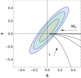
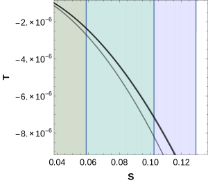
Figure 1: Allowed values for $T$ and $S$ for LEP data at 68% (gray), 95% (pale green) and 99% (violet). Plots for $S$ vs $T$ are given for $r-1=10^{-4},10^{-3},5\cdot 10{-3},10^{-2}$ and $0.5$ on the left-hand-side figure. Plots for $S$ vs $T$ with a zoom into the figure of the left-hand-side for $r=2,3,4,5$ on the right-hand-side. Notice that the plots converge rapidly for $r\geq 3$.

Bounds on the vector resonance mass can be obtained using the experimentally allowed regions for $S$ and $T$ for different confidence levels. Notice that as $r$ grows, $T$ converges rapidly to the limit

$$\lim_{r\,\to\,\infty}T=-\pi\frac{v^{2}\left(m_{Z}^{2}-m_{W}^{2}\right)}{M_{V}^{4}}\,\,\frac{m_{Z}^{2}}{m_{W}^{2}}=-4.5\cdot 10^{-4}\left(\frac{1\text{ TeV}^{4}}{M_{V}^{4}}\right).$$ (36)

This effect can be noted in the right-hand-side plot of Figure 1, where $r=3$ is sufficiently close to $r\to\infty$. The experimental limits given for $S$ and $T$ allow us to give bounds on $M_{V}$ for different values of $r$, shown in Table 2. Notice that, although one loop corrections are neglected in these estimates, they might become relevant for the T parameter in more general analyses [20, 21].

$r=M_{A}^{2}/M_{V}^{2}$		lower bound	for $M_{V}$
		68%CL	95%CL
$1+10^{-3}$		$5.2$ TeV	$4.0$ TeV
$1.1$		$5.1$ TeV	$3.9$ TeV
$2$		$4.5$ TeV	$3.4$ TeV
$\infty$		$3.7$ TeV	$2.8$ TeV

Table 2: Bounds on $M_{V}$ for different values of $r$ using the allowed region for $S$ and $T$ using the 68% and 95% confidence level data from LEP [4].

6 Conclusions

In the framework of Chiral Electroweak Lagrangians, a simple explanation to the strong suppression of fermionic BSM operators is proposed. This suppression stems from the fact that BSM operators appear due to the exchange of resonances which do not couple directly to the SM fermions. This means an extra suppression due to additional exchange of gauge bosons. Thus, in the case of the four-fermion (Fermi-like) operators, the contact interaction in eq. (34), in addition to the naive expected value $1/M_{V}^{2}$, carries an additional suppression factor of the form

$$\frac{4m_{Z}^{4}-8m_{Z}^{2}m_{W}^{2}+7m_{W}^{4}}{24v^{2}M_{V}^{2}}=9.6\cdot 10^{-5}\left(\frac{\text{1 TeV}^{2}}{M_{V}^{2}}\right).$$ (37)

As seen from Table 1, a stringent bound on the four-fermion parameter $\Lambda$ does not automatically imply an equally stringent bound on BSM heavy states masses. We note, nevertheless, that the results in Table 1 are just rough estimates. A full four-fermion operator analysis should be performed in both the theoretical and experimental sides.

In order to give more reliable bounds on the masses of BSM spin 1 fields we used the experimental limits on the oblique $S$ and $T$ parameters from LEP [4]. Considering NLO terms in the equations of motion of the resonances we obtained terms that break custodial symmetry, inducing thus a non-vanishing contribution to the oblique $T$ parameter. It can be seen from eq. (34) that $T$ (NLO) is suppressed with respect to $S$ (LO), as one would expect from contributions actually arising at different orders in perturbation theory.

The bounds on $M_{V}$ for different values of $r=M_{A}^{2}/M_{V}^{2}$ obtained in this way show that BSM resonances with masses $M_{R}\sim 1$ TeV are still compatible with experimental limits, and are also compatible with the bounds obtained through fermionic observables regarding these resonances do no couple directly to the SM fermions.

References

• [1] F. Alvarado, A. Guevara and J. J. Sanz Cillero, in preparation.
• [2] M. Aaboud et al. [ATLAS Collaboration], Phys. Rev. D 96 (2017) no.5, 052004.
• [3] A. M. Sirunyan et al. [CMS Collaboration], JHEP 1707 (2017) 013.
• [4] S. Schael et al. [ALEPH and DELPHI and L3 and OPAL and LEP Electroweak Collaborations], Phys. Rept.  532 (2013) 119.
• [5] M. E. Peskin and T. Takeuchi, Phys. Rev. Lett.  65 (1990) 964.
• [6] M. E. Peskin and T. Takeuchi, Phys. Rev. D 46 (1992) 381.
• [7] G. Altarelli and R. Barbieri, Phys. Lett. B 253 (1991) 161.
• [8] G. Altarelli, R. Barbieri and S. Jadach, Nucl. Phys. B 369 (1992) 3; Erratum: [Nucl. Phys. B 376 (1992) 444].
• [9] S. Weinberg, Physica A 96 (1979) 327.
• [10] J. Gasser and H. Leutwyler, Annals Phys.  158 (1984) 142.
• [11] J. Gasser and H. Leutwyler, Nucl. Phys. B 250 (1985) 465.
• [12] A. Pich, I. Rosell, J. Santos and J. J. Sanz-Cillero, JHEP 1704 (2017) 012.
• [13] C. Krause, A. Pich, I. Rosell, J. Santos and J. J. Sanz-Cillero, JHEP 1905 (2019) 092.
• [14] G. Ecker, J. Gasser, A. Pich and E. de Rafael, Nucl. Phys. B 321 (1989) 311.
• [15] G. Ecker, J. Gasser, H. Leutwyler, A. Pich and E. de Rafael, Phys. Lett. B 223 (1989) 425.
• [16] S. R. Coleman, J. Wess and B. Zumino, Phys. Rev.  177 (1969) 2239.
• [17] C. G. Callan, Jr., S. R. Coleman, J. Wess and B. Zumino, Phys. Rev.  177 (1969) 2247.
• [18] M. J. Herrero and E. Ruiz Morales, Nucl. Phys. B 418 (1994) 431.
• [19] S. Weinberg, Phys. Rev. Lett.  18 (1967) 507.
• [20] A. Pich, I. Rosell and J. J. Sanz-Cillero, JHEP 1401 (2014) 157.
• [21] A. Pich, I. Rosell and J. J. Sanz-Cillero, Phys. Rev. Lett.  110 (2013) 181801.