Tripartite entanglement: Foundations and applications

Abstract

We review some current ideas about tripartite entanglement, the case representing the next level of complexity beyond the simplest one (though far from trivial), namely the bipartite. This kind of entanglement has an essential role in the understanding of foundations of quantum mechanics. Also, it allows several applications in the fields of quantum information processing and quantum computing. In this paper, we make a revision about the main foundational aspects of tripartite entanglement and we discuss the possibility of using it as a resource to execute quantum protocols. We present some examples of quantum protocols in detail.
$\rightarrow$ This version contains an Erratum: $\rightarrow$ We fix some mistakes presented in the previous version.

I Introduction

Quantum entanglement is one of most astonishing aspects of Quantum Mechanics, initially due to the deep implications in the context of the theory itself and more recently because of the large amount of applications within the emerging fields of Quantum Information [1] and Quantum Computation.

The most well-known type of entanglement involves two parts sharing two qubits, namely, the EPR or sometimes called Bell states [3]. Nevertheless, note that two parts may also share an entangled state in larger dimensions, like qutrits [4].

Besides the relevance of bipartite entanglement in the understanding of quantum foundations and quantum information science, the search of entangled states involving more than two qubits is also desirable, because it opens new possibilities on the fundamental aspects of the theory itself and also in development of new protocols in Quantum Information [5]. Also, dealing with genuine multipartite entanglement can provide several advantages in comparison with bipartite entanglement [6]. It is possible to establish quantum networks with multi-users, execute quantum computation by using cluster states [7, 8] and also perform measurement-based quantum computing [9]. These entangled states could be used, for instance, as a quantum channel to establish quantum communication between several separated locations.

The simplest case of multipartite entanglement it is tripartite entanglement, that involves three-parts. These type of entanglement have an essential role in the development of aspects like quantum non-locality and a large number of applications in quantum information protocols. In this review, we explore the main features of tripartite entanglement, from the most fundamental aspects to applications.

The paper is organized in the following way: In section 2, we consider a brief overview of bipartite entanglement. In section 3, we make a discussion about tripartite entanglement and define the corresponding classes of entanglement for qubits. Then, we consider some aspects of quantum non-locality and tripartite entanglement in section 4. In section 5, we consider several examples of quantum information protocols employing tripartite entanglement. We review the main aspects of these applications, illustrating the corresponding schemes. In section 6, we list several contributions to the production of tripartite entanglement in the literature. Then, we proceed considering the detection and characterization of tripartite entanglement in section 7. In section 8, we consider the topic of Remote Preparation of quantum states. In section 9, we include aspects of tripartite entanglement involving continuous variables. The effects of noisy environments it is considered in section 10. Finally, we make our conclusions in section 11.

II Overview on Bipartite Entanglement

For the sake of completeness, let us quickly review some important aspects of entanglement between two parts. We start by describing the case of pure states and then we cite some of the most important entangled mixed states.

II.1 Pure states

Due to the Schmidt decomposition, any quantum state shared between two parts, say Alice and Bob as usual, may be written as $\ket{\psi}=\sum_{j=0}^{d-1}\sqrt{\lambda_{j}}\ket{\phi_{A}}_{j}\otimes\ket{\varphi_{B}}_{j}=\sum_{j=0}^{d-1}\sqrt{\lambda_{j}}\ket{j,j}$, with Schmidt coefficients $\lambda_{j}\in\mathbb{R}$, satisfying $\sum_{j=0}^{d-1}\lambda_{j}=1$ and $d=\min(\dim{\mathcal{H}_{A},\dim{\mathcal{H}_{B})}}$, where $\mathcal{H}_{k}$ is the Hilbert space associated to the $k-$th part. In particular, it is possible to say that $\ket{\psi}$ is entangled whenever there exist more than one non-null Schmidt coefficients. Furthermore, we can define a basis for the Hilbert space associated to both parts $\mathcal{H}_{AB}=\mathcal{H}_{A}\otimes\mathcal{H}_{B}$, composed by $d^{2}$ elements given by

$$\ket{\phi_{mn}^{(d)}}=\sum_{k=0}^{d-1}\omega_{d}^{mk}\beta_{km}\ket{k,k\oplus n},\;\;\;\;\;m,n=0,\dots,d-1,$$ (1)

where $\omega_{d}=\exp(2\pi i/d)$ is the primitive $d$-th root of unity, the symbol “$\oplus$” denotes sum modulo $d$ and the $\beta_{km}$ coefficients control how entangled the basis is. In particular, for $d=2$ the basis can be parametrized as [11]

$$\ket{\phi_{00}^{(2)}}=\cos\theta\ket{00}+\sin\theta\ket{11},\;\;\;\;\;\ket{\phi_{10}^{(2)}}=\sin\theta\ket{00}-\cos\theta\ket{11},$$

$$\ket{\phi_{01}^{(2)}}=\cos\theta\ket{01}+\sin\theta\ket{10},\;\;\;\;\;\ket{\phi_{11}^{(2)}}=\sin\theta\ket{01}-\cos\theta\ket{10},$$

with $0\leq\theta\leq\pi/2$. Moreover any element of the basis with $\beta_{km}=1/\sqrt{d}$ corresponds to a maximally entangled state. Explicitly, it is known as Bell or EPR basis for $d=2$

$$\ket{\phi^{\pm}}=\frac{1}{\sqrt{2}}\left(\ket{00}\pm\ket{11}\right),\hskip 11.38092pt\ket{\psi^{\pm}}=\frac{1}{\sqrt{2}}\left[\ket{01}\pm\ket{10}\right].$$ (2)

Hereafter $\ket{\phi_{mn}^{(d)}}$ denotes a maximally entangled state, for the sake of simplicity.

An important feature is that any Bell state can be converted into another one by using local unitary transformations and classical communication (hereafter LOCC). Moreover, it has been shown that these states can be used to develop several informational tasks such as superdense coding and quantum teleportation with the highest attainable performance, and also represent a very useful resource in tests to investigate fundamental aspects of the quantum world.

II.2 Some special families of mixed states

Suppose Alice and Bob have a source of entangled qudits prepared in a state $\hat{\rho}$. Then, she applies an unitary operation $\hat{U}$ chosen at random and informs Bob to carry out either $\hat{U}$ or $\hat{U}^{*}$ on his qudit. Regardless the initial state of the system, after many repetitions of the same procedure, the final state shared by Alice and Bob reduces to a Werner or an isotropic state.

II.2.1 Werner states

When Alice and Bob apply local operations $\hat{U}\otimes\hat{U}$, we have [14]

$$\hat{\rho}\rightarrow\int\hat{U}\otimes\hat{U}~{}\hat{\rho}~{}\hat{U}^{\dagger}\otimes\hat{U}^{\dagger}\differential U=\hat{\rho}_{W},$$ (3)

where $\differential U$ is the Haar measure of the unitary group $\textbf{U}(d)$ and $\hat{\rho}_{W}$ is the Werner state, given by

$$\hat{\rho}_{W}=(1-p)\frac{2}{d^{2}+d}\hat{P}^{(+)}+p\frac{2}{d^{2}-d}\hat{P}^{(-)},$$ (4)

with $\hat{P}^{(\pm)}=\frac{1}{2}\left(\hat{1}\pm\hat{V}\right)$, where $\hat{1}$ is the identity: $\hat{1}=\sum_{jk=0}^{d-1}\outerproduct{jk}{jk}$ and $\hat{V}$ is the flip operator: $\hat{V}=\sum_{jk=0}^{d-1}\outerproduct{jk}{kj}$. It is important to mention that the Werner state $\hat{\rho}_{W}$ is invariant under $\hat{U}\otimes\hat{U}$ operations. By using the following relations $\hat{P}^{(+)}\hat{P}^{(-)}=0$, $\hat{P}^{(\pm)2}=\hat{P}^{(\pm)}$ and $\tr\hat{P}^{(-)}=\frac{1}{2}(\tr\hat{1}-\tr\hat{V})=\frac{1}{2}(d^{2}-d)$, it is easy to show that the operation invariant $p$ is equal to $p=\tr(\hat{P}^{(-)}\hat{\rho}_{W})$.

II.2.2 Isotropic states

In the case of local operations $\hat{U}\otimes\hat{U}^{*}$, the state $\hat{\rho}$ is transformed as [16]

$$\hat{\rho}\rightarrow\int\hat{U}\otimes\hat{U^{*}}~{}\hat{\rho}~{}\left(\hat{U}\otimes\hat{U^{*}}\right)^{\dagger}\differential U=\hat{\rho}_{f},$$ (5)

where $\hat{\rho}_{f}$ is the isotropic state, given by

$$\hat{\rho}_{f}=\frac{1-f}{d^{2}-1}\hat{1}+\frac{fd^{2}-1}{d^{2}-1}\hat{P}_{+},$$ (6)

with $\hat{P}_{+}=\outerproduct{\phi_{00}^{(d)}}{\phi_{00}^{(d)}}$. Analogously to the Werner state, the isotropic state is invariant under $\hat{U}\otimes\hat{U}^{*}$ operations.

By expanding the identity operator in the generalized Bell basis $\hat{1}=\sum_{\mu\nu=0}^{d-1}\outerproduct{\phi_{\mu\nu}^{(d)}}{\phi_{\mu\nu}^{(d)}}$, the isotropic state takes the following form:

$$\hat{\rho}_{f}=f\outerproduct{\phi_{00}^{(d)}}{\phi_{00}^{(d)}}+\frac{1-f}{d^{2}-1}\sum_{\begin{subarray}{c}\mu\nu=0\\ (\mu,\nu)\neq(0,0)\end{subarray}}^{d-1}\outerproduct{\phi_{\mu\nu}^{(d)}}{\phi_{\mu\nu}^{(d)}}.$$ (7)

In this expression it is possible to see more clearly that the operation invariant $f$ is equal to: $f=\tr(\outerproduct{\phi_{00}^{(d)}}{\phi_{00}^{(d)}}\hat{\rho})=\tr(\outerproduct{\phi_{00}^{(d)}9}{\phi_{00}^{(d)}}\hat{\rho}_{f})$. Due to their properties, these states have been very useful to unveil the relation between the concepts of entanglement and Bell non-locality [17, 18]. Several proposed generalizations to the multipartite case are exposed later in this review.

III Tripartite entanglement

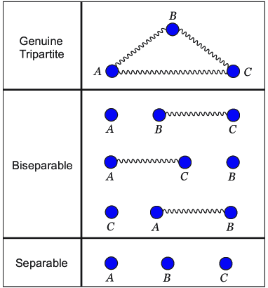
Figure 1: All the possibilities of how entangle three qubits. From the top to the bellow: First, Genuine tripartite entanglement, where all qubits are in a entangled state. Second, it is possible to have biseparable states, where two qubits are entangled, and another one it is separated. Third, three qubits in a state full separable.

III.1 Genuine tripartite pure states

When dealing with tripartite quantum systems it is possible to write the associated state $\ket{\Psi}$, in one out of three ways: totally separable $\ket{\Psi}=\ket{\psi_{A}}\otimes\ket{\psi_{B}}\otimes\ket{\psi_{C}}$, biseparable partitions $\ket{\Psi}=\ket{\psi_{j}}\otimes\ket{\psi_{kl}}$ ($\{j,k,l\}=\{A,B,C\}$) or genuinely entangled, explained in the next part. In [19], Zhao and collaborators provide a set of methods based on expectation values of Pauli operators to identify the class of a given state.

It is a well known fact that it is possible to transform any state from the Bell basis into anther one by using LOCC only, or to another arbitrary state of two qubits with non-null probability [20, 21]. However, a very interesting feature emerges when we deal with quantum systems involving more than two qubits: different classes of entanglement arise. For the simplest instance, namely three qubits, there are two inequivalent classes of entanglement [22]: GHZ states [23, 24] and W states [22, 25], defined as

$$\ket{GHZ}=\frac{1}{\sqrt{2}}\left(\ket{000}+\ket{111}\right),\;\;\;\;\;\;\;\;\ket{W}=\frac{1}{\sqrt{3}}\left(\ket{001}+\ket{010}+\ket{100}\right).$$ (8)

These two classes are totally inequivalent under Stochastic Local Operations and Communication (hereafter SLOCC). It means that it is impossible to convert any state of a given class into another one and vice-versa. Thus, GHZ and W states constitute Genuinely Entangled states for the case of three qubits.

The idea of GHZ entanglement by itself has its deep origins in the foundations of Quantum Theory. In fact, this family of states was proposed to investigate quantum non-locality beyond Bell’s Theorem [24], as showed in [26], the premises of the EPR argument about the incompleteness of Quantum Theory are also inconsistent when applied to GHZ states. As discussed in more details in upcoming sections, the employment of GHZ states led to the possibility to demonstrate the incompatibility between predictions of local realism and quantum mechanics without demanding the usage of an inequality [3].

As in the bipartite case, it is also possible to write a GHZ state with arbitrary amount of entanglement. In this case, we start by defining the state

$$\ket{\psi_{000}}=\cos\theta\ket{000}+\sin\theta\ket{111},$$ (9)

with $\theta=\{0,\pi/2\}$. From local operations on $\ket{\psi_{000}}$, we can construct a GHZ basis. These states are given by

$$\ket{\psi_{\mu\lambda\omega}}=\sum_{j}(-1)^{\mu j}b_{\mu\oplus j}\ket{j,j\oplus\lambda,j\oplus\omega},$$ (10)

where $b_{0}=\cos\theta$ e $b_{1}=\sin\theta$. More explicitly:

$$\ket{\psi_{000}}=\cos\theta\ket{000}+\sin\theta\ket{111},\;\;\;\;\;\ket{\psi_{001}}=\cos\theta\ket{001}+\sin\theta\ket{110},$$ (11)

$$\ket{\psi_{010}}=\cos\theta\ket{010}+\sin\theta\ket{101},\;\;\;\;\;\ket{\psi_{011}}=\cos\theta\ket{011}+\sin\theta\ket{100},$$ (12)

$$\ket{\psi_{100}}=\sin\theta\ket{000}-\cos\theta\ket{111},\;\;\;\;\;\ket{\psi_{101}}=\sin\theta\ket{001}-\cos\theta\ket{110},$$ (13)

$$\ket{\psi_{110}}=\sin\theta\ket{010}-\cos\theta\ket{101},\;\;\;\;\;\ket{\psi_{111}}=\sin\theta\ket{011}-\cos\theta\ket{100}.$$ (14)

In the same way, we can also define a more general family of entangled W states, given by [27]:

$$\left|W_{1}\right\rangle=\sin\theta\cos\varphi\left|001\right\rangle+\sin\theta\sin\varphi\left|010\right\rangle+\cos\theta\left|100\right\rangle.$$ (15)

By using local unitary operations, we can generate the other seven states of the W basis:

$$\left|W_{2}\right\rangle=+\sin\theta\sin\varphi\left|001\right\rangle-\sin\theta\cos\varphi\left|010\right\rangle+\cos\theta\left|111\right\rangle,$$ (16)

$$\left|W_{3}\right\rangle=-\sin\theta\sin\varphi\left|100\right\rangle+\cos\theta\left|010\right\rangle+\sin\theta\cos\varphi\left|111\right\rangle,$$ (17)

$$\left|W_{4}\right\rangle=+\sin\theta\cos\varphi\left|100\right\rangle+\cos\theta\left|001\right\rangle+\sin\theta\sin\varphi\left|111\right\rangle,$$ (18)

$$\left|W_{5}\right\rangle=+\sin\theta\cos\varphi\left|110\right\rangle+\sin\theta\sin\varphi\left|101\right\rangle+\cos\theta\left|011\right\rangle,$$ (19)

$$\left|W_{6}\right\rangle=+\sin\theta\sin\varphi\left|110\right\rangle-\sin\theta\cos\varphi\left|101\right\rangle+\cos\theta\left|000\right\rangle,$$ (20)

$$\left|W_{7}\right\rangle=-\sin\theta\sin\varphi\left|011\right\rangle+\cos\theta\left|101\right\rangle+\sin\theta\cos\varphi\left|000\right\rangle,$$ (21)

$$\left|W_{8}\right\rangle=+\sin\theta\cos\varphi\left|011\right\rangle+\cos\theta\left|110\right\rangle+\sin\theta\sin\varphi\left|000\right\rangle.$$ (22)

Let us consider the partial trace operation on the third qubit in $\psi_{000}$ and $\ket{W_{1}}$, in order to examine the differences between the two classes. A simple calculation gives us

$$\hat{\rho}_{12}=\tr_{3}\left(\outerproduct{\psi_{000}}{\psi_{000}}\right)=\frac{1}{2}\outerproduct{00}{00}+\frac{1}{2}\outerproduct{11}{11},$$ (23)

for the GHZ state. For the W state, we have

$$\hat{\rho}_{12}=\tr_{3}\left(\outerproduct{W}{W}\right)=\frac{2}{3}\outerproduct{\phi_{01}^{(2)}}{\phi_{01}^{(2)}}+\frac{1}{3}\outerproduct{00}{00}.$$ (24)

Thus, in the case of a W state, the reduced density operator contains a residual EPR entanglement, in contrast, the same operation on the GHZ state gives a completely disentangled state.

III.2 Other instances of tripartite entanglement

In analogy with the bipartite case, Acín and collaborators [28], defined a Schmidt-like decomposition useful to classify pure three-qubits states [29]. These results were after generalized to include mixed states [30].

In addition to the cases mentioned above, there are several instances of tripartite entanglement. For instance, in [31], it is presented a procedure to create a tripartite GHZ entangled states in three levels for every particle. In [32], Siewer and Eltschka use the following generalization of the Werner states

$$\hat{\varrho}_{W}=p\outerproduct{\psi_{000}}{\psi_{000}}+\frac{1}{8}(1-p)\hat{1}_{8},$$ (25)

to treat the problem of entanglement quantification.

III.3 Tripartite entanglement in other areas

It is worth to note that there are several works exploring the idea of entanglement and its classification with other fields in Physics and Mathematics. For instance, there are some works discussing on relationship between entanglement and topology. A connection between Borromean rings and GHZ states was established by Aravind in [33]. In [34], it is presented a schematic comparison between GHZ and W tripartite states by using knots. There have been efforts to unveil the relation between quantum entanglement and topological entanglement [35, 36]. A recent review about this topic can be found in [37]. The idea of entanglement in networks also has been explored.

In [38], it is presented a strategy for percolation involving GHZ states. In [39], it was presented an experimental verification of three and four-party entanglement in quantum networks.

A connection between black-hole physics and quantum entanglement was presented in [40]. This work also shows that there is a matching between the classification of tripartite entanglement and black holes. A more recent work concerning this topic is [41].

Several works in the literature have been reported focusing on the use of both GHZ and W classes as quantum resources to develop quantum protocols, such as Quantum Teleportation and Superdense Coding. In fact, as we will see, the two classes work in a different way depending on the specific task.

IV Non locality, Bell’s Theorem and GHZ states

Besides the success of Quantum Theory describing systems in the microscopic world and all the experimental tests in its favour, the foundations of the theory have been widely discussed since its proposal. Albert Einstein, working with Boris Podolsky and Nathan Rosen, for instance, questioned whether Quantum Mechanics could give a complete description of the physical reality. In a paper published in 1935, they established their famous EPR paradox. In their work, EPR conceived an experiment in which Alice and Bob share an ensemble of entangled pairs of qubits, and each of them is able to perform local measurements. Under this scenario, the measurement events are separated by space-like intervals. At each instant Alice may choose one out of two incompatible observables $\hat{A}_{1}$ or $\hat{A}_{2}$ (analogously for Bob, $\hat{B}_{1}$ or $\hat{B}_{2}$). Assuming that any local action on each particle cannot influence its counterpart (locality), and that measurement results pre-exist for any observable independent of the choice (realism), they were able to show that under special cases concerning systems with a high degree of symmetry, two local measurements (one in Alice and the other in Bob’s location) allow for the determination of the values associated to the four involved observables, and thus in contradiction with Heisenberg’s uncertainty principle. EPR concluded that there is no way in which QM satisfy the local realism assumption, and then there should exist a more general theory possibly described by a set of hidden variables (not available for the experimenter), in analogy to the relation between thermodynamics and statistical mechanics, in which the position of particles in the phase space play the role of hidden variables. Inspired by this, Bell derived a set of conditions (Bell inequalities) satisfied by predictions from any theory based on local hidden variables, which as mentioned before, quantum mechanics violates under certain scenarios [43]. Since then many efforts have been concentrated to experimentally test Quantum Theory against the local realism hypothesis, with a vast majority in favor of the first one. For a recent revision on the subject, we refer the reader to [17].

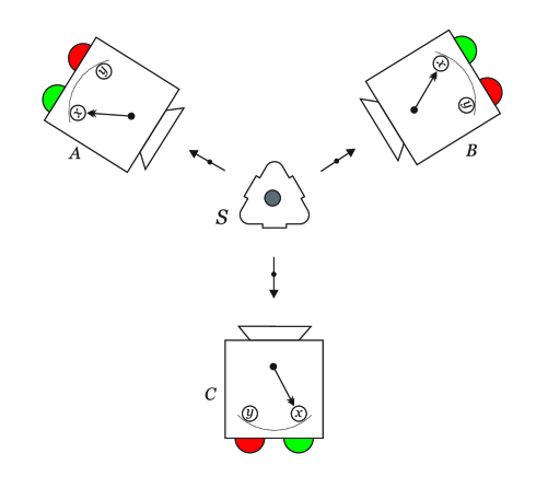
Figure 2: Bell nonlocality in a tripartite scenario. A source S emits three spin $1/2$ particles, traveling to one out of three different detectors located in A, B and C. Each part, namely Alice, Bob and Charlie posses a Stern-Gerlach magnet, and can choose make a $\hat{\sigma}_{x}$ or $\hat{\sigma}_{y}$ measurement, obtaining the eigenvalues $+1$ or $-1$, corresponding to turn on green or red lights.

Now, let us analyze the conflict between local realism and the predictions of Quantum Mechanics by employing a GHZ state. This analysis was initially proposed by Greenberger, Horne and Zeillinger. Here, we present an alternative version by Mermin [44]. For an intuitive introduction, see also [3, 45]. An interesting extension which covers W states is given in [46].

First of all, recall the following relations, valid for a single qubit:

$$\hat{\sigma}_{x}\ket{0}=\ket{1},\;\;\;\;\;\;\hat{\sigma}_{x}\ket{1}=\ket{0},\;\;\;\;\;\;\hat{\sigma}_{y}\ket{0}=i\ket{1},\;\;\;\;\;\;\hat{\sigma}_{y}\ket{1}=-i\ket{0}.$$ (26)

Consider three parties, Alice, Bob and Charlie sharing a GHZ state $\ket{\psi_{100}}$.

Let calculate $(\hat{\sigma}_{x}\otimes\hat{\sigma}_{y}\otimes\hat{\sigma}_{y})\ket{\psi_{100}}$. It means that Alice, Bob and Charlie apply $\hat{\sigma}_{x}$, $\hat{\sigma}_{y}$ and $\hat{\sigma}_{y}$, locally on their qubits respectively. This calculation gives

$$\hat{\sigma}_{x}\otimes\hat{\sigma}_{y}\otimes\hat{\sigma}_{y}\ket{\psi_{100}}=\frac{1}{\sqrt{2}}\hat{\sigma}_{x}\otimes\hat{\sigma}_{y}\otimes\hat{\sigma}_{y}\left(\ket{000}+\ket{111}\right)=-1\ket{\psi_{100}}.$$ (27)

Thus the GHZ state is an eigenstate of $\hat{\sigma}_{x}\otimes\hat{\sigma}_{y}\otimes\hat{\sigma}_{y}$, with eigenvalue $-1$. By using the notation employed in [3], we can say that the product

$$m_{x}^{A}m_{y}^{B}m_{y}^{C}=-1,$$ (28)

where, $m_{x}^{A}=\pm 1$ indicates the result of the operation $\hat{\sigma}_{x}$ on Alice’s qubit, for example.

We can also calculate $\hat{\sigma}_{y}\otimes\hat{\sigma}_{x}\otimes\hat{\sigma}_{y}\ket{\psi_{100}}$ and $\hat{\sigma}_{y}\otimes\hat{\sigma}_{x}\otimes\hat{\sigma}_{x}\ket{\psi_{100}}$, obtaining the same result, $-1$. In this way we can also write the outcome products as

$$m_{y}^{A}m_{x}^{B}m_{y}^{C}=-1,~{}~{}~{}~{}~{}~{}~{}m_{y}^{A}m_{y}^{B}m_{x}^{C}=-1.$$ (29)

The product of the three terms in Eqs. 28 and 29, holds:

$$m_{x}^{A}m_{y}^{B}m_{y}^{C}m_{y}^{A}m_{x}^{B}m_{y}^{C}m_{y}^{A}m_{y}^{B}m_{x}^{C}=m_{x}^{A}m_{x}^{B}m_{x}^{C}=-1.$$ (30)

Note that in the last calculations we used the fact that $\left(m_{y}^{A}\right)^{2}=\left(m_{y}^{B}\right)^{2}=\left(m_{y}^{C}\right)^{2}=+1.$ Moreover, the calculation of $\hat{\sigma}_{x}\otimes\hat{\sigma}_{x}\otimes\hat{\sigma}_{x}\ket{\psi_{100}}$ leads to a quite different result: $+1\ket{\psi_{100}}$, which implies that

$$m_{x}^{A}m_{x}^{B}m_{x}^{C}=+1.$$ (31)

Thus, we have a contradiction between Eqs. 30 and 31. It indicates the fundamental impossibility to associate pre-determined outcomes for every local measurement performed on a quantum entangled state. In fact, the so called GHZ paradox constitutes the first proof of a possible violation of local realism without the usage of an inequality. Furthermore, it is possible to find generalized versions of Bell inequalities for tripartite case. For instance, Mermin, Ardehali, Belinski and Klyshko (MABK) derived independently a set of inequalities capable of testing violation of local realism for a states of $N$ spin-$1/2$ particles [48, 49, 50]. In addition, Svetlichny made an important contribution to the understanding of genuine tripartite nonlocality [51]. In his work, it was presented for the first time an inequality that allows the detection of genuine nonlocality in scenarios involving three observers, each capable of performing one out of two dichotomic measurements. In [52] it is discussed the notion of tripartite entanglement in contrast with that of nonlocality in the context of the Svetlichny inequality. See also [53], for a definition of genuine multipartite nonlocality alternative to original Svetlichny’s proposal. An more recent discussion about tripartite genuine nonlocality can be found in [54].

Tripartite entangled states have widely been used to test the previsions of Quantum Theory over Local Hidden Variables Models. For instance, in [55], was reported a experimental test of quantum nonlocality with GHZ states. An experimental setup to generate GHZ states and test the Svetlichny inequality was also reported in [56]. In [57], it was presented the experimental verification of Mermin’s inequality violations by distributing tripartite GHZ states between independent observers. This work closed locality and freedom-of-choice loopholes for three particles. In [58], it was reported an experimental study on quantum nonlocality by dealing with W states. In [59], it was made an analysis of nonlocality robustness of GHZ and W states under noisy conditions and weak measurements. An experimental demonstration of Mermin’s and Svetlichny’s inequalities for GHZ and W states was discussed in [60]. In [61], it was studied the violation of Svetlichny inequality in the presence of several kinds of noise for the case of GHZ states.

More recently Chaves, Cavalcanti and Aolita, by using the formalism of Bayesian networks have found new different expressions of nonlocality on tripartite states [62].

V Quantum information protocols using three-partite entanglement

Tripartite entanglement can be widely used to execute tasks in the field of quantum information. In this section, we give examples of applicability of this type of entanglement in some protocols.

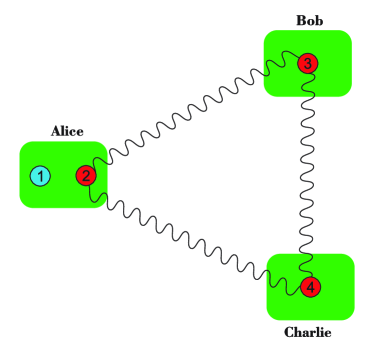
Figure 3: A possible scheme to make a teleport of a qubit state by using a three-particle entangled state as the quantum channel.

V.1 Teleportation of a single qubit state by using a GHZ channel and EPR measurements

Attention: This section contains a mistake. Please consider the Erratum at the and of the manuscript.

A scheme to make a quantum teleport of a qubit state by using a GHZ state as the channel was reported in [63]. In this scheme, there are three users, namely Alice, Bob, and Charlie, as shown in figure 3. They shared a GHZ state. Alice has a non-shared qubit, whose state she wants to teleport. The state of the system is

$$\ket{\Psi}=[\alpha\ket{0}+\beta\ket{1}]_{1}\otimes\frac{1}{\sqrt{2}}[\ket{000}+\ket{111}]_{234}.$$ (32)

We can write this state in a more compact form as

$$\ket{\Psi}=\sum_{i=0}^{1}\alpha_{i}\ket{i}_{1}\otimes\sum_{j=0}^{1}\frac{1}{\sqrt{2}}\ket{jjj}_{234}.$$ (33)

In this case, Alice makes a Bell-measurement on the qubits 1 and 2. This way, let us separate the qubits in the following way:

$$\ket{\Psi}=\frac{1}{\sqrt{2}}\sum_{i,j}\alpha_{i}\ket{ij}_{12}\ket{jj}_{34}.$$ (34)

Let us calculate the projection of $\ket{\Psi}$ into the $m,n$ element of the EPR basis on qubits 1 and 2, $\bra{\phi_{mn}^{(2)}}_{12}$. It holds

$$\bra{\phi_{mn}}_{12}\hskip 1.42271pt\ket{\Psi}=\ket{\eta}_{34}=\frac{1}{2}\sum_{ijk}\alpha_{i}(-1)^{mk}\left\langle k,k\oplus n|i,j\right\rangle_{12}\otimes\ket{j,j}_{34}.$$ (35)

As result, Charlie and Bob, now, share an EPR state:

$$\ket{\eta}_{34}=\ket{\eta_{mn}}_{34}=\sum_{k=0}^{1}(-1)^{mk}\alpha_{k}\ket{k,k\oplus n}_{34}.$$ (36)

This EPR state it is not necessarily $\ket{\Phi^{+}}$. Actually, it can be any one of the four sttates of the EPR basis. Which state Charlie and Bob will share have a dependence on Alice’s measurement result. It is important to note that the new state shared by Charlie and Bob it is not a perfect EPR state because the coefficients of this state are $\alpha_{0}$ and $\alpha_{1}$. If Alice obtains the state $\ket{\psi_{00}},$ for instance, Bob and Charlie share the state

$$\ket{\eta_{00}}_{34}=\sum_{k}\alpha_{k}\ket{k,k}=\alpha_{0}\ket{00}+\alpha_{1}\ket{11}.$$ (37)

Table 1: Results after Alice’s measurement and the states that Bob and Charlie shares.

Alice’s result		State shared by Bob and Charlie
$m$	$n$	state
0	0	$\ket{\eta_{00}}=\alpha_{0}\ket{00}+\alpha_{1}\ket{11}$
0	1	$\ket{\eta_{01}}=\alpha_{0}\ket{01}+\alpha_{1}\ket{10}$
1	0	$\ket{\eta_{10}}=\alpha_{0}\ket{00}-\alpha_{1}\ket{11}$
1	1	$\ket{\eta_{11}}=\alpha_{0}\ket{01}-\alpha_{1}\ket{10}$

The table 4 exhibits the states that can be shared by Bob and Charlie after Alice’s measurement. Let us explore in more details the case $\ket{\eta_{00}}.$ As shown in [63], to proceed with the protocol, Bob or Charlie should make a measurement on a single qubit. Let us suppose that Alice wants to teleport the state of her qubit to Charlie. Then, she asks Bob to make a measurement on his qubit. Bob uses the following basis:

$$\ket{0}_{3}=\sin\theta\ket{x_{0}}_{3}+\cos\theta\ket{x_{1}}_{3},\;\;\;\;\;\ket{1}_{3}=\cos\theta\ket{x_{0}}_{3}-\sin\theta\ket{x_{1}}_{3}.$$ (38)

Replacing these expressions on the equation 98, we have:

$$\ket{\eta_{00}}_{34}=\alpha_{0}(\sin\theta\ket{x_{1}}_{3}+\cos\theta\ket{x_{2}}_{3})\ket{0}_{4}+\alpha_{1}(\cos\theta\ket{x_{1}}_{3}-\sin\theta\ket{x_{2}}_{3})\ket{0}_{4}.$$ (39)

We can reorganize the expression as

$$\ket{\eta_{00}}_{34}=\ket{x_{1}}_{3}(\alpha_{0}\sin\theta\ket{0}_{4}+\alpha_{1}\cos\theta\ket{1}_{4})+\ket{x_{2}}_{3}(\alpha_{0}\cos\theta\ket{0}_{4}-\alpha_{1}\sin\theta\ket{1}_{4}).$$ (40)

Thus, if Bob measures $\ket{x_{1}},$ the state (up to normalization) is $\alpha_{0}\sin\theta\ket{0}_{4}+\alpha_{1}\cos\theta\ket{1}_{4}$. The table 4 shows all possibilities after Alice’s measurement and Bob’s measurement.

Table 2: Alice’s and Bob’s results; and the final state obtained by Charlie.

Alice’s result		Bob’s result	State (unnormalized) of Charlie’s qubit
$m$	$n$	$\ket{x_{i}}$	state
0	0	$\ket{x_{0}}$	$\alpha_{0}\sin\theta\ket{0}+\alpha_{1}\cos\theta\ket{1}$
0	0	$\ket{x_{1}}$	$\alpha_{0}\cos\theta\ket{0}-\alpha_{1}\sin\theta\ket{1}$
0	1	$\ket{x_{0}}$	$\alpha_{0}\sin\theta\ket{1}+\alpha_{1}\cos\theta\ket{0}$
0	1	$\ket{x_{1}}$	$\alpha_{0}\cos\theta\ket{1}-\alpha_{1}\sin\theta\ket{0}$
1	0	$\ket{x_{0}}$	$\alpha_{0}\sin\theta\ket{0}-\alpha_{1}\cos\theta\ket{1}$
1	0	$\ket{x_{1}}$	$\alpha_{0}\cos\theta\ket{0}+\alpha_{1}\sin\theta\ket{1}$
1	1	$\ket{x_{0}}$	$\alpha_{0}\sin\theta\ket{1}-\alpha_{1}\cos\theta\ket{0}$
1	1	$\ket{x_{1}}$	$\alpha_{0}\cos\theta\ket{1}+\alpha_{1}\sin\theta\ket{0}$

Table 3: Alice’s and Bob’s results; and the corresponding operations needed to recover the desired state.

Result:   $(m,n,i)$	Operation
$(0,0,0)$	$\hat{I}$
$(0,0,1)$	$\hat{\sigma}_{z}$
$(0,1,0)$	$\hat{\sigma}_{x}$
$(0,1,1)$	$\hat{\sigma}_{z}\hat{\sigma}_{x}$
$(1,0,0)$	$\hat{\sigma}_{z}$
$(1,0,1)$	$\hat{I}$
$(1,1,0)$	$\hat{\sigma}_{z}\hat{\sigma}_{x}$
$(1,1,1)$	$\hat{\sigma}_{x}$

We can write the state of Bob’s qubit, before his measurement, as

$$\ket{k}_{3}=\sum_{j=0}^{1}(-1)^{jk}b_{j\oplus k}\ket{x_{j}}_{3}.$$ (41)

Here, we have defined

$$b_{0}\equiv\sin\theta,\hskip 11.38092ptb_{1}=\cos\theta.$$ (42)

This way,

$$\ket{\eta_{mn}}_{34}=\sum_{k=0}^{1}(-1)^{mk}\alpha_{k}\left(\sum_{j=0}^{1}(-1)^{jk}b_{j\oplus k}\ket{x_{j}}_{3}\right)\ket{k\oplus n}_{4}.$$ (43)

Essentially, this expression contains the same information showed on the table 4. To obtain the final state of Charlie’s qubit, we can calculate the projection of the above state on $\ket{x_{\ell}}$, where $\ell=0,1.$

$$\ket{\chi_{mn0}}_{4}=\bra{x_{0}}_{3}\hskip 1.42271pt\ket{\eta_{mn}}_{34}=\sum_{k=0}^{1}(-1)^{mk}\alpha_{k}b_{k}\ket{k\oplus n}.$$ (44)

$$\ket{\chi_{mn1}}_{4}=\bra{x_{1}}_{3}\hskip 1.42271pt\ket{\eta_{mn}}_{34}=\sum_{k=0}^{1}(-1)^{(m\oplus 1)k}\alpha_{k}b_{k\oplus 1}\ket{k\oplus n}.$$ (45)

The indexes $mn0$ and $mn1$ are related with the measurements of Alice and Bob on their qubits. These index are the same showed in table 5. To recover the desired state, Charlie needs to apply a unitary transformation on his qubit. Which unitary he will use, depends of $(m,n,i)$. The table 6 shows list of the operations for all results. For the case $(0,0,0)$, for example, the state (up to normalization) is

$$\ket{\chi_{000}}=\alpha_{0}\sin\theta\ket{0}_{4}+\alpha_{1}\cos\theta\ket{1}_{4}.$$ (46)

In this case, the operation is the identity. The normalized state is

$$\ket{\chi_{000}}_{f}=\frac{\alpha_{0}\sin\theta\ket{0}_{4}+\alpha_{1}\cos\theta\ket{1}_{4}}{\sqrt{|\alpha_{0}|^{2}\sin^{2}\theta+|\alpha_{1}|^{2}\cos^{2}\theta}}.$$ (47)

Let’s see what happens when the result is $(0,0,1).$ In this case, the state, up to normalization, is

$$\ket{\chi_{001}}=\alpha_{0}\cos\theta\ket{0}_{4}-\alpha_{1}\sin\theta\ket{1}_{4};$$ (48)

Now, Charlie needs to apply the $\hat{\sigma}_{z}$ operation on his qubit to recover the desired state. We can note that

$$\hat{\sigma}_{z}\ket{\chi_{001}}=\alpha_{0}\cos\theta\ket{0}_{4}+\alpha_{1}\sin\theta\ket{1}_{4}.$$ (49)

After the normalization, we have

$$\ket{\chi_{001}}_{f}=\frac{\alpha_{0}\cos\theta\ket{0}_{4}+\alpha_{1}\sin\theta\ket{1}_{4}}{\sqrt{|\alpha_{0}|^{2}\cos^{2}\theta+|\alpha_{1}|^{2}\sin^{2}\theta}}.$$ (50)

All the results can be viewed on tables 4 and 6. Another work dealing with GHZ states as the quantum channel can be accessed in [64].

V.2 Teleportation of a single qubit state: GHZ channel and measurement

Another possibility to use GHZ states in quantum teleportation is by employing a GHZ channel and making a GHZ measurement on Alice’s side. An example of a protocol dealing with GHZ measurements can be viewed in [65]. Let us suppose that, now, Alice wants to teleport of a single qubit, and shares a GHZ entangled state with Bob. Let us consider that Alice has two qubits of the shared GHZ state, and Bob has another one. Thus, now Alice has three qubits and Bob has one. To diversify the mathematical approach used here, let us now write the states by using the formalism of the density matrix. This problem has been discussed in [66], where was considered a maximally entangled state as the channel as well in the measurement. It was showed that this procedure can help to improve the quality of the protocol on the occurrence of bit-flip error. Here, let us consider non-maximally entangled GHZ states. It is interesting to consider such states, because, we can see how the quality of the entanglement affects the final results. The effect of dealing with non-maximally GHZ entangled states also can be viewed in other scenarios. In [67], for instance, has addressed the problem of sharing a multiqubit state using non-maximally GHZ entangled states.

Figure 4: Scheme to teleport a single qubit state by using a GHZ state as the quantum channel. A GHZ measurement it is taken on the qubits 1, 2, 3.

Alice wants to teleport the state

$$\ket{\phi}=c_{0}\ket{0}+c_{1}\ket{1}=\sum_{i=0}^{1}c_{i}\ket{i}.$$ (51)

The corresponding density operator is given by

$$\hat{\rho}_{1}=\sum_{ij}c_{i}c_{j}^{*}\ket{i}\bra{j}.$$ (52)

Let us consider that the channel is given by $\ket{\Phi^{+}}_{ghz}=\beta_{0}\ket{000}+\beta_{1}\ket{111},$ where $\beta_{0}=\cos\theta$ and $\beta_{1}=\sin\theta.$ We can write this state as

$$\ket{\Phi^{+}}_{ghz}=\sum_{k=0}^{1}\beta_{k}\ket{kkk}.$$ (53)

The corresponding density operator is

$$\hat{\rho}_{234}=\sum_{k\ell}\beta_{k}\beta_{\ell}\ket{kkk}\bra{\ell\ell\ell}.$$ (54)

The state of the whole system is

$$\hat{\rho}=\hat{\rho}_{1}\otimes\hat{\rho}_{234}=\sum_{ijk\ell}c_{i}c_{j}^{*}\beta_{k}\beta_{\ell}\ket{ikkk}_{1234}\bra{j\ell\ell\ell}_{1234}.$$ (55)

Let us separate the qubits that will taken on the GHZ measurement.

$$\hat{\rho}=\hat{\rho}_{1}\otimes\hat{\rho}_{234}=\sum_{ijk\ell}c_{i}c_{j}^{*}\beta_{k}\beta_{\ell}\ket{ikk}_{123}\bra{j\ell\ell}_{123}\otimes\ket{k}_{4}\bra{\ell}_{4}.$$ (56)

To the measurement, we will consider the basis introduced in Eq. 10.

After the measurement, the unnormalized state is given by

$$\tilde{\rho}_{I}(\mu,\lambda,\omega)=\sum_{j^{\prime}k^{\prime}}(-1)^{\mu j^{\prime}}(-1)^{\mu k^{\prime}}b_{\mu\oplus j^{\prime}}b_{\mu\oplus k^{\prime}}\beta_{k^{\prime}\oplus\lambda}\beta_{j^{\prime}\oplus\lambda}\delta_{\lambda,\omega}c_{k^{\prime}}c_{j^{\prime}}^{*}\ket{k^{\prime}\oplus\lambda}_{4}\bra{j^{\prime}\oplus\lambda}_{4}.$$ (57)

This state depends on the parameters related to the measurement, $(\mu,\lambda,\omega)$. For the case where $(\mu,\lambda,\omega)=(0,0,0)$, for example, we have

$$\tilde{\rho}_{I}(0,0,0)=\sum_{j^{\prime}k^{\prime}}(b_{j^{\prime}}b_{k^{\prime}}\beta_{j^{\prime}}\beta_{k^{\prime}}\delta_{\lambda,\omega})c_{k^{\prime}}c_{j^{\prime}}^{*}\ket{k^{\prime}}\bra{j^{\prime}}.$$ (58)

More explicitly,

$$\tilde{\rho}_{I}(0,0,0)=b_{0}^{2}\beta_{0}^{2}|c_{0}|^{2}\ket{0}\bra{0}+b_{1}^{2}\beta_{1}^{2}|c_{1}|^{2}\ket{1}\bra{1}+b_{0}b_{1}\beta_{0}\beta_{1}(c_{0}c_{1}^{*}\ket{0}\bra{1}+c_{1}c_{0}^{*}\ket{1}\bra{0}).$$ (59)

By the other hand,

$$\tilde{\rho}_{I}(1,1,1)=\sum_{j^{\prime}k^{\prime}}(-1)^{j^{\prime}}(-1)^{k^{\prime}}b_{j^{\prime}\oplus 1}b_{k^{\prime}\oplus 1}\beta_{k^{\prime}\oplus 1}\beta_{j^{\prime}\oplus 1}\delta_{\lambda,\omega}c_{k^{\prime}}c_{j^{\prime}}^{*}\ket{k^{\prime}\oplus 1}_{4}\bra{j^{\prime}\oplus 1}_{4},$$ (60)

or

$$\tilde{\rho}_{I}(1,1,1)=b_{1}^{2}\beta_{1}^{2}|c_{0}|^{2}\ket{1}\bra{1}+b_{0}^{2}\beta_{0}^{2}|c_{1}|^{2}\ket{0}\bra{0}-b_{0}b_{1}\beta_{0}\beta_{1}(c_{1}c_{0}^{*}\ket{0}\bra{1}+c_{0}c_{1}^{*}\ket{1}\bra{0}).$$ (61)

The normalized state after the measurement is given by

$$\hat{\rho}_{I}=\hat{\rho}_{I}(\mu,\lambda,\omega)=\frac{\hat{P}\hat{\rho}_{0}\hat{P}^{\dagger}}{P}=\frac{\tilde{\rho}_{I}}{P},$$ (62)

where

$$\hat{P}=\hat{P}_{\mu\lambda\omega}=(\ket{\Phi^{\mu}_{\lambda}}\bra{\Phi^{\mu}_{\lambda\omega}})_{123}$$ (63)

is the projector associated to GHZ measurement, and

$$P=P_{\mu\lambda\delta\omega}=Tr(\hat{P}\hat{\rho}_{0})$$ (64)

corresponds to probability of each outcome.

Each outcome $(\mu,\lambda,\omega)$ requires a unitary transformation, in order to recover the desired state. In the case $(0,0,0)$, the operation it is just the identity. In the case $(1,1,1)$, Bob needs to apply $\hat{\sigma}_{z}\hat{\sigma}_{x}.$ Looking to the expression to $\tilde{\rho}_{I}$, it is possible to suggest that the general form of operation needed is given by

$$\hat{U}=\hat{U}_{\mu\lambda\omega}=(\hat{\sigma}_{z})^{\mu}(\hat{\sigma}_{x})^{\lambda}.$$ (65)

After the measurement, by using a classical channel, Alice informs Bob which $\mu$ and $\lambda$ are needed to recover the desired state. We can check if this operation works by calculating $\hat{U}\tilde{\rho}_{I}\hat{U}^{\dagger}.$

$$\tilde{\rho}_{f}=\hat{U}\tilde{\rho}_{I}\hat{U}^{\dagger}=\sum_{j^{\prime}k^{\prime}}b_{\mu\oplus j^{\prime}}b_{\mu\oplus k^{\prime}}\beta_{k^{\prime}\oplus\lambda}\beta_{j^{\prime}\oplus\lambda}\delta_{\lambda,\omega}c_{k^{\prime}}c_{j^{\prime}}^{*}\ket{k^{\prime}}\bra{j^{\prime}}.$$ (66)

This way, the unitary corrects the factor $k^{\prime}\oplus\lambda$ on the ket and the factor $(-1)^{\mu k^{\prime}}$. However, it is impossible to correct the factors involving $b$ and $\beta$.

The fidelity correspondent to a specific outcome is

$$F_{\mu\lambda\omega}=Tr(\hat{\rho}_{in}\tilde{\rho}_{f}).$$ (67)

The average fidelity is

$$\overline{F}=\sum_{\mu\lambda\omega}P_{\mu\lambda\omega}F_{\mu\lambda\omega}=\sum_{\mu\lambda\omega}P_{\mu\lambda\omega}Tr[\hat{\rho}_{in}\hat{\rho}_{f}].$$ (68)

Here, ${\rho}_{f}$ is the final state, after the unitary transformation. When we deal with maximally entangled states, we know that the probability of obtaining a specific outcome it is the same than the others (the probability it is the same for all outcomes.) It is not true in more general cases. Then, this average fidelity takes into account that, when we deal with non-maximally entangled states, the probability of obtaining an outcome depends on the amount of entanglement. Also, each outcome has a different probability. In this case, we need to sum all the contributions of each outcome times the correspondent statistical weight $P_{\mu\lambda\omega}$. But,

$$\hat{\rho}_{f}=\frac{\hat{U}\tilde{\hat{\rho}}_{I}\hat{U}^{\dagger}}{P_{\mu\lambda\omega}}=\frac{\tilde{\rho}_{f}}{P_{\mu\lambda\omega}}.$$ (69)

Thus,

$$\overline{F}=\sum_{\mu\lambda\omega}Tr[\hat{\rho}_{in}\tilde{\rho}_{f}],$$ (70)

or

$$\overline{F}=\sum_{k\ell\mu\nu\lambda\omega}|c_{k}|^{2}|c_{\ell}|^{2}b_{\mu\oplus k}^{*}b_{\mu\oplus\ell}\beta_{k\oplus\lambda}\beta_{\ell\oplus\lambda}.$$ (71)

Making all the sums, we have

$$\overline{F}=|c_{0}|^{4}+|c_{1}|^{4}+2|c_{0}|^{2}|c_{1}|^{2}\left(b_{0}b_{1}\beta_{0}\beta_{1}\right).$$ (72)

The expression above depends on the initial state. In order to obtain a quantity independent of the parameters of the initial state, let us consider that the initial state can be parametrized as

$$\ket{\Psi}_{in}=\left|c_{0}\right|\ket{000}+\left|c_{1}\right|e^{i\varphi}\ket{111},$$ (73)

in a such way we can now calculate a average on all possible input states:

$$\langle\overline{F}\rangle=\frac{1}{2\pi}\int_{0}^{2\pi}\int_{0}^{1}\overline{F}(|c_{0}|^{2},\varphi)d|c_{0}|^{2}d\varphi.$$ (74)

Evaluating the integral, we obtain

$$\langle\overline{F}\rangle=\frac{2}{3}+\frac{1}{3}\sin(2\theta)\sin(2\phi).$$ (75)

In this expression, the first term corresponds to the classical contribution, and the second one depends on the entanglement of the channel and of measurement basis. Essentially, it has the same form that the fidelity for the standard teleportation protocol, using EPR channel and measurement. However, as pointed in [66], in the presence of bit-flip noise, GHZ states allow correction of error. This way, it is possible to improve fidelity.

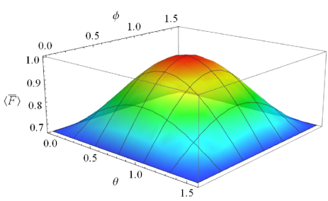
Figure 5: Graph of the quantum fidelity corresponding to the case of a single-qubit state teleport by using a GHZ channel, as function of entanglement of the channel as well the entanglement of measurement basis.

The figure 5 shows the plot of the fidelity as a function of $\theta$ and $\phi$. When the states on the channel and in the measurement basis are maximally entanglement, the maximum of fidelity is reached, corresponding to $\langle\overline{F}\rangle=1$, the perfect case.

V.3 Teleportation of a two-qubit state

An interesting quantum teleportation protocols consist in making a teleport of a two-qubits entangled state [68]. In [69], was proposed a scheme to teleport an EPR-like state by using GHZ states as the channel. Others schemes also have been proposed, like in [70, 71]. Recently, it was showed a scheme to teleport an arbitrary two-qubit state by using two GHZ states [72]. In [73], it was exhibited a protocol to teleport a two-qubit state by using a both GHZ and W states simultaneously as the quantum channel. The teleport of an EPR state by a non-maximally entangled GHZ quantum channel was discussed in [74]. In [75], was shown a scheme to make bidirectional teleportation of an EPR state using GHZ states. In [76], a protocol dealing with a composite channel using EPR and GHZ states is presented, to execute a multihop teleport of a two-qubit state. In the reference [77], it was presented a scheme to teleport an arbitrary two-qubit state by using a channel consisting of a tripartite entangled state (GHZ or W) and an EPR state.

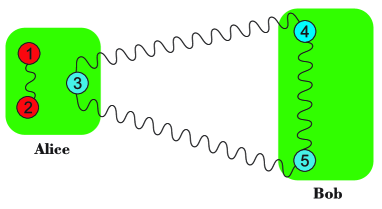
Figure 6: An EPR state can be teleported by using a GHZ state as the quantum channel. A measurement on GHZ basis also it is considered.

The figure 6 shows a possible scheme to teleport a EPR state. A GHZ state can be used as the quantum channel, and a measurement in a GHZ-basis on the qubits 1, 2 and 3 it is taken. The state of the system is

$$(a_{0}\ket{00}+a_{1}\ket{11})_{12}\otimes\frac{1}{\sqrt{2}}(\ket{000}+\ket{111})_{345}.$$ (76)

V.4 Teleportation of a GHZ state

Another possibility of quantum teleportation protocol it is the teleport of a GHZ state. It is an interesting issue, because besides make a teleport of information itself, the protocol also provides quantum entanglement to other locations. It is relevant in the sense that the distribution of entanglement could be used, in principle, to connect several distant users in a quantum network, for example. Several works have been addressed to this problem. In [78], was investigated the teleportation of GHZ state with N photons by using a two-photon entangled state as the quantum channel. A scheme to teleport a GHZ state via entanglement-swapping is showed in [79]. The teleportation of a GHZ state by using two W entangled states as the quantum channel was considered in [80]. GHZ states also can be transmitted through a multihop teleportation scheme by using Bell’s states as intermediate quantum channels [81]. In [82], was proposed a scheme to teleport a GHZ-like state by employing three pairs of non-maximally entangled states as the quantum channel. The configuration to make the protocol is illustrated in figure 7. In [83], a similar protocol to the last one was presented, but this time to teleport an arbitrary tripartite state.

Figure 7: A possible scheme to teleport a GHZ state. Three EPR states are used as the quantum channel, and EPR measurements are taken on qubits 1, 4 and 2, 6 and 3, 8. At the end, the qubits 5, 7, 9 are in a GHZ state.

The figure 7 shows a possible scheme to make a teleport of a GHZ state by using three EPR states as the quantum channel. The state of the system is given by

$$\ket{\Psi}=\ket{\phi}_{123}\otimes\ket{\eta}_{45}\otimes\ket{\chi}_{67}\otimes\ket{\zeta}_{89},$$ (77)

where

$$\ket{\phi}_{123}=a_{0}\ket{000}_{123}+a_{1}\ket{111}_{123},$$ (78)

$$\ket{\eta}_{45}=\sum_{j}b_{j}\ket{jj}_{45},\hskip 14.22636pt\ket{\chi}_{67}=\sum_{k}c_{k}\ket{kk}_{67},\hskip 14.22636pt\ket{\zeta}_{89}=\sum_{\ell}x_{\ell}\ket{\ell\ell}_{89}.$$ (79)

In this scheme, Alice makes three EPR measurements on her side. The measurements are taken on the particles (1,4), (2,6) and (3,8). The reference [82] shows the procedure in details to finish the protocol.

V.5 Teleportation of a single qubit state using a W channel

In [84], was reported a possible scheme to deal with a single qubit state teleportation by employing a W state as the channel and an EPR measurement. In this work, was showed that W states are suitable to make the protocol probabilistically. In this work, there were some wrong calculations about the probabilities. It was set by [85] and [86]. However, besides the conclusion presented in [84] is correct, the calculations for the case of a W state with the generic state it is not quite precise. In the following, we explicit the correct calculations for a teleport of a qubit state by using a generic W state. The state to be teleported is

$$\ket{\phi}_{1}=\alpha\ket{0}_{1}+\beta\ket{1}_{1}.$$ (80)

The channel is

$$\ket{W}_{234}=a\ket{100}_{234}+b\ket{010}_{234}+c\ket{001}_{234}.$$ (81)

The general state of the system is

$$\ket{\Psi}=[\alpha\ket{0}+\beta\ket{1}]_{1}\otimes\left[a\ket{100}+b\ket{010}+c\ket{001}\right]_{234}.$$ (82)

More explicitly, we have

$$\ket{\Psi} =\alpha a\ket{0100}_{1234}+\alpha b\ket{0010}_{1234}+\alpha c\ket{0001}_{1234}$$

$$+\beta a\ket{1100}_{1234}+\beta b\ket{1010}_{1234}+\beta c\ket{1001}_{1234}.$$ (83)

Now, we can write the states of qubits 1 and 2 in terms of the EPR basis.

$$\left|\Psi\right\rangle =\frac{\alpha a}{\sqrt{2}}\left(\left|\psi^{+}\right\rangle+\left|\psi^{-}\right\rangle\right)_{12}\left|00\right\rangle_{34}+\frac{\alpha b}{\sqrt{2}}\left(\left|\Phi^{+}\right\rangle+\left|\Phi^{-}\right\rangle\right)_{12}\left|10\right\rangle_{34}$$

$$+\,\frac{\alpha c}{\sqrt{2}}\left(\left|\Phi^{+}\right\rangle+\left|\Phi^{-}\right\rangle\right)_{12}\left|01\right\rangle_{34}+\frac{\beta a}{\sqrt{2}}\left(\left|\Phi^{+}\right\rangle-\left|\Phi^{-}\right\rangle\right)_{12}\left|00\right\rangle_{34}$$

$$+\frac{\beta b}{\sqrt{2}}\left(\left|\psi^{+}\right\rangle-\left|\psi^{-}\right\rangle\right)_{12}\left|10\right\rangle_{34}+\frac{\beta c}{\sqrt{2}}\left(\left|\psi^{+}\right\rangle-\left|\psi^{-}\right\rangle\right)_{12}\left|01\right\rangle_{34};$$ (84)

We can write this expression in the following way:

$$\left|\Psi\right\rangle =\frac{\left|\Phi^{+}\right\rangle_{12}}{\sqrt{2}}[\alpha b\left|10\right\rangle+\alpha c\left|01\right\rangle+\beta a\left|00\right\rangle]_{34}+\frac{\left|\Phi^{-}\right\rangle_{12}}{\sqrt{2}}[\alpha b\left|10\right\rangle+\alpha c\left|01\right\rangle-\beta a\left|00\right\rangle]_{34}$$

$$+\frac{\left|\psi^{+}\right\rangle_{12}}{\sqrt{2}}[\alpha a\left|00\right\rangle+\beta b\left|10\right\rangle+\beta c\left|01\right\rangle]_{34}+\frac{\left|\psi^{-}\right\rangle_{12}}{\sqrt{2}}[\alpha a\left|00\right\rangle-\beta b\left|10\right\rangle-\beta c\left|01\right\rangle]_{34}.$$

By separating the qubits 3 and 4, results

$$\left|\Psi\right\rangle =\frac{\left|\Phi^{+}\right\rangle_{12}}{\sqrt{2}}\Biggl{[}\Biggl{(}\alpha b\left|1\right\rangle_{3}+\beta a\left|0\right\rangle_{3}\Biggl{)}\left|0\right\rangle_{4}+\alpha c\left|0\right\rangle_{3}\left|1\right\rangle_{4}\Biggl{]}$$

$$+\frac{\left|\Phi^{-}\right\rangle_{12}}{\sqrt{2}}\Biggl{[}\Biggl{(}\alpha b\left|1\right\rangle_{3}-\beta a\left|0\right\rangle_{3}\Biggl{)}\left|0\right\rangle_{4}+\alpha c\left|0\right\rangle_{3}\left|1\right\rangle_{4}\Biggl{]}$$

$$+\frac{\left|\psi^{+}\right\rangle_{12}}{\sqrt{2}}\Biggl{[}\Biggl{(}\alpha a\left|0\right\rangle_{3}+\beta b\left|1\right\rangle_{3}\Biggl{)}\left|0\right\rangle_{4}+\beta c\left|0\right\rangle_{3}\left|1\right\rangle_{4}\Biggl{]}$$

$$+\frac{\left|\psi^{-}\right\rangle_{12}}{\sqrt{2}}\Biggl{[}\Biggl{(}\alpha a\left|0\right\rangle_{3}-\beta b\left|1\right\rangle_{3}\Biggl{)}\left|0\right\rangle_{4}-\beta c\left|0\right\rangle_{3}\left|1\right\rangle_{4}\Biggl{]}.$$

Let us suppose that, after a measurement on qubits 1 and 2 in the EPR basis, Alice obtains $\left|\psi^{+}\right\rangle$. In this case, the unnormalized state of qubits 3 and 4 is given by

$$\frac{1}{\sqrt{2}}\Biggl{[}\Biggl{(}\alpha a\left|0\right\rangle_{3}+\beta b\left|a\right\rangle_{3}\Biggl{)}\left|0\right\rangle_{4}+\beta c\left|0\right\rangle_{3}\left|1\right\rangle_{4}\Biggl{]}.$$ (87)

It’s worth to note that the joint-state of the qubits 3 and 4 also contains EPR entanglement. This way, after a single qubit measurement, it is possible to complete the protocol. If the qubit 4 it is projected on the $\left|0\right\rangle$ state, then the state of qubit 3 (up to normalization) it will be $\left|\eta\right\rangle_{3}=\alpha a\left|0\right\rangle_{3}+\beta b\left|1\right\rangle_{3}.$ This state looks like the initial state $\ket{\phi}_{1}$. However, there is a imperfection due the coefficients $a$ and $b$. We can say that the initial state was teleported, but containing a imperfection. By other hand, if the qubit 4 it is projected on the state $\left|1\right\rangle$, then there is no teleport. This way, we can conclude that the protocol works probabilistically. Another works investigating the using of W states as the quantum channel [87] were reported. In [88], the teleport of a single qubit state also was analyzed. Posteriorly, a important contribution was reported in [89], where was showed that there is type of W states that can be used for perfect teleportation and superdense coding. A generalization of that work it was reported in [90]. In [91], a composite W-Bell channel is used to execute quantum teleportation and superdense coding protocols.

V.6 Teleportation of a W state

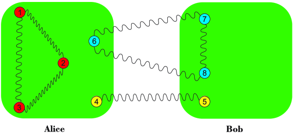
Figure 8: A possible way to teleport a W state it is illustrated. A GHZ state and an EPR channel are used as the quantum channel.

A quantum teleportation scheme of a tripartite W state it was presented in [92]. In that scheme, Alice wants to teleport the state

$$\ket{\phi}_{123}=x\ket{001}_{123}+y\ket{010}_{123}+z\ket{100}_{123},$$ (88)

on the particles 1, 2, 3. She shares two entangled states with Bob, a GHZ state and a EPR state, that will be used as the quantum channels. The EPR state is given by

$$\ket{\psi}_{45}=a_{0}\ket{00}_{45}+a_{1}\ket{11}_{45},$$ (89)

and the GHZ state is

$$\ket{\eta}_{678}=c_{0}\ket{000}_{678}+c_{1}\ket{111}_{678}.$$ (90)

The state of the whole system is

$$\ket{\Psi}=\ket{\phi}_{123}\otimes\ket{\psi}_{45}\otimes\ket{\eta}_{678}.$$ (91)

The particles 1, 2, 3, 4 and 6 are on the Alice’s side, while particles 5, 7 and 8 are on Bob’s side. To execute the teleport, two EPR measurements are taken, on the particles 1, 6 and 3, 4. After the measurements, the resultant state involves the particles 2, 5, 7 and 8. Thus, it is necessary to trace out the particle 2. However, in order to complete the protocol, it is not make directly. Here, the protocol it is more complicated than the previous one we have discussed. Now, it is needed to employ combinations of Hadamard gate, CNOT gate and the introduction of a auxiliary particle. All procedures to do that are presented in the reference [92]. More recently, another scheme to teleport a W state was reported in the reference [93], where two W states are used as the quantum channel.

V.7 Dense coding

The original Dense Coding it was presented by using a two-entangled state as the resource, but tripartite entanglement also it is suitable to make the protocol works [94], and several schemes have been proposed. Two examples of controlled dense coding dealing with GHZ states can be accessed in [95, 96]. The W state also it is suitable to make a controlled dense coding protocol [97]. A recent study about Super Dense Coding with W states can be accessed in [98]. In [99], was proposed a scheme to implement Dense coding protocol by using tripartite entanglement in cavity QED. In [100] it was analyzed the use of GHZ and W states to make Deterministic Dense Coding.

V.8 Quantum cryptography and Quantum Secure Communication

Quantum Mechanics can also be used to perform cryptographic protocols. The basis of this field are founded by Wiensner [101]. Posteriorly, other fundamental steps were due to C. Bennet and G. Brassard (scheme known as BB84 protocol) [102] and A. Ekert [103]. After these initial developments, the use of Multipartite Entanglement has been considered. In [104], it was shown that a GHZ state can be used to make the Quantum Secret Sharing protocol. In [105], it was presented some variants of protocols of quantum secure communication dealing with W states.

Schemes to establish a three-party quantum secure communication using GHZ states are reported in [106, 107]. In [108], it proposed a protocol for quantum secure direct communication utilizing W states.

V.9 Other developments

In [109], it was presented a quantum protocol to send and receive messages anonymously where $n$ players have a access a shared $n$-qubit GHZ entangles state. Recently, it was reported a scheme to transmit a anonymous message in a network employing W-type states with N qubits [110]. In [111], it were proposed quantum algorithms to the generation of GHZ and W states of $n$ qubtis to be used on quantum networks. In [112], tripartite entanglement it is examined in a noninertial frame when one of the parties is subjected to a uniform acceleration. Tripartite entanglement also has been studied in the context of distillation of entanglement.

Methods of distillation of GHZ states can be accessed in [113, 114]. Protocols for the optimal distillation of W states were reported in [115]. In [116], it is presented a method for entanglement purification of three-qubit states by using weak measurements. In [117], it was showed a distillation of GHZ-type states from two copies of a mixed state in a single step.

The relationship between tripartite entanglement and quantum computing also can be explored. In [118], it was demonstrated that a GHZ state can be uses as an ingredient in the construction of a universal quantum computer. The relationship between state complexity and quantum computing is discussed in [119], including GHZ and W states in the analysis. A discussion about the computational power of GHZ and W states can be accessed in [120]. In [121], it was proposed a conceptual design for a quantum block-chain by using a temporal entangled GHZ state.

VI Production of three-partite entanglement

The production of multipartite entanglement have been attracted much attention. An experimental demonstration of five-qubits entanglement it was realized by Zhao and collaborators [122] in 2004. In 2011, Huang and colleagues have reported an experimental realization of an eight-photon GHZ state. In the same year, the creation of an entangled state of 14-qubit also it was presented [123]. The first experimental production of of a three-photon GHZ state was reported in 1999 [124]. Recently, the deterministic generation of a 18-qubit entangled GHZ state it was achieved. An experimental realization of a W state was reported in [125]. In [126] it was reported a pioneer scheme for generating three-particle entanglements, using just two pairs of entangled particles from independent emissions. Another pioneer work involving GHZ states it was due to Bouwmeester and colleagues [124], observing the GHZ entanglement for three qubits in the polarization degree of freedom of photons. In [127], it was described the creation of maximally entangled GHZ states using Nuclear Magnetic Resonance (NMR). Since then, several works has been proposed, employing different frameworks. A proposal for creation of GHZ and W states via quantum walks, for instance, can be accessed in [128]. In [129], it was presented a scheme to generate multipartite entanglement by using a single-neutron interferometer. In [130] was proposed a scheme to preparation of a W state using Parametric Down-Conversion. Schemes to prepare GHZ and W states of three distant atoms were reported in [131]. A method to generate a $n$-qubit W state in cavity QED it was reported in [132]. In [133], a scheme to prepare W states from atomic ensembles it is presented. The creation of GHZ and W states with a trapped-ion quantum computer was reported in [134]. The preparation of spin-qubit GHZ and W states in a quantum-dot-microcavity system it was discussed in [135]. It is also possible generate W states of three superconducting qubits [136]. A scheme to generate entanglement between three atoms trapped in cavities via quantum Zeno dynamics it was proposed in [137]. In [138], we can see a scheme to generate GHZ and W states from cavities with Jaynes–Cummings Hamiltonians. In [139], it was showed a procedure to generate three-photon polarization entanglement, and is made the characterization of the produced states. Such states are used to make tests of local realism. Recently, a scheme to generate GHZ states encoded on the path degree of freedom of three photons was presented in [140]. Another recent proposal for the generation of tripartite entanglement can be accessed in [141], where the creation of W states employing cross-Kerr nonlinearity and quantum dots it is addressed. The production of larger states involving multi-qubits it is desirable to make protocols involving quantum networks [39]. Several steps has been achieved in this direction. A scalable scheme to create W states, for example, it was presented in 2017 [142]. In [143], it was presented a deterministic scheme for preparing W states of size of any power of 2. A scheme to prepare a $N$-qubit GHZ state in a chain of four-level Rydberg atoms it was proposed in [144] recently. In [145], it was demonstrate the creation of entangled states with up to 20 qubits.

VII Detection and characterization of tripartite entanglement

The detection of multipartite entanglement it is a hard task [146]. Several efforts, theoretical and experimental, has been done to improve the methods to make it. The entanglement detection involves a key ingredient: the construction of Entanglement Witness [147, 148] . In several practical situations, it is possible to certify entanglement through the violation of some inequality that indicates nonlocality. However, the number of inequalities increases when the number of qubits increases. While a measure of nonlocality depends on correlations, an Entanglement Witnesses it is an operator, corresponding to a physical observable. The first GHZ state-analyzer was proposed in [149], where two of the eight GHZ states can be distinguished using linear optical elements. After this first step, several contributions have been reported. In the [150], it is presented a scheme for the universal tripartite GHZ-state analyzer using two-photon polarization QND parity detectors based on the weak nonlinearity. The method allows discrimination of all the eight states with a probability near to the unity. In [152], a method to construct a nondestructive n-qubit GHZ-state analyzer it is presented. A GHZ state analyzer using only linear-optics elements through hyperentangled states with polarization and momentum degrees of freedom can be viewed in [154]. Another scheme involving GHZ hyperentangled states it was recently proposed [155].

In [156], it was investigated the existence of tripartite entanglement in a noninteracting Fermi gas, and some Entanglement Witness are introduced in that scenario. A recent study about separability criteria of three-qubit GHZ state can be accessed in [157]. In [158] are established sufficient conditions for detecting genuine tripartite entanglement, providing an operational point of view to measure and detect this type of entanglement. Experimental schemes to identify the entanglement classes of tripartite states can be accessed in [159, 160].

A powerful tool to describe a density matrix of a system it is the method known as quantum state tomography, that allows the characterization of a quantum state [161]. These methods have been employed in the study of tripartite entangled states. In [162], it was realized an experimental tomographic reconstruction of a three-photon polarization GHZ state. A more recent work using the method for GHZ states it is the reference [163]. In [164], it was reported a scheme of experimental generation of a W state, and its full characterization by using quantum state tomography method.

VIII Remote preparation

Besides the quantum teleportation protocol, another type of protocol dealing with the quantum state transfer it is the Remote Preparation Protocols (RSP) [165]. Several possibilities of RSP can be done, involving different kinds of channels. It is possible to think in RSP to prepare single-qubit states, and also states with two or more qubits [166]. Currently, this topic has been studied considering the preparation of multipartite entangled states. It is an interesting task since the production of entanglement remotely can help in using this resource to establish quantum communication between distant multi-users and establish quantum distributed computation [167]. In [168], it was presented a scheme for remote preparation of a four-qubit GHZ state through two non-maximally entangled three-qubit GHZ states. The remote preparation of a three-qubit state by using GHZ state it was considered in [169]. In [170], GHZ are used as the quantum channel for the remote preparation of arbitrary states of one and two qubits. A scheme for preparing atomic states remotely by using GHZ states it is also possible [171]. In [172], W states are used for remote preparation of single and two-qubit states. In [173], two maximally entangled GHZ states are used as the quantum channel for the remote preparation of an arbitrary equatorial two-qubit state. A scheme for remote preparation of a two-qubit state by using two W-type states as the quantum channel also it was reported [174]. The remote preparation of $m$-qubit states by using non-maximally GHZ entangled state it was studied in [175]. In [176], it was reported an experimental demonstration of remote preparation of three-photon entangled states by using a single photon measurement. In [177], it was presented a scheme to joint remote preparation of a $m$-qudit state by using a $d$-dimensional GHZ state. In [178], EPR pairs are used as the quantum channel to the preparation of an arbitrary three-qubit state. Tripartite entangled states not only can be used to remote preparation of single and two-qubit states, but they also can be themselves remotely prepared. In [179], it was presented a scheme for preparing W states remotely by using two four-particle GHZ states as the quantum channel. A proposal to remote preparation of a three-particle state employing a three-particle orthonormal basis projective measurement can be accessed in [180]. An idea for remotely preparing W states of three and four-qubit utilizing tripartite GHZ states it was presented in [181]. In [182], it was reported an efficient scheme for remote preparation of a $2^{n}$-qubit W state via $n$ three-qubit GHZ states. A scheme to prepare a tripartite equatorial state by using three maximally entangled GHZ states it was proposed in [183]. In [184], it was presented a protocol to remotely preparing a tripartite W-type state by using an eight-qubit state as the quantum resource.

IX Continuous-variable systems

Until this point, we have explored several aspects involving tripartite entanglement of discrete variables, that refers to qubit-based developments, like photon polarization or the spin of electron. It is worth to note that, it is also possible dealing with multipartite entangled states in the domain of continuous variables [185, 186]. Several quantum information protocols has been considered in that domain, where the variables has a continuous spectrum of eigenvalues. For instance, an analysis of quantum teleportation of quantum states with continuous variables was presented in [187]. In [188], an experimental investigation of this subject was reported. The entanglement swapping involving continuous variables was investigated in [189] and [190]. A study approaching necessary conditions of separability of a multiparty continuous-variable state can be viewed in [191]. A detailed discussion about quantum information and continuous variables it is presented in [192]. A complete analysis of three-mode Gaussian entangled states it is showed in [193]. In that work, the counterparts of GHZ and W states in the continuous-variable scenario are presented. Experimentally, the creation of a tripartite entangled state in continuous-variables it is reality [194]. In [195], it was demonstrated the generation of entanglement among three beams of light with different wavelengths. In [196], there is a experimental demonstration of tripartite entanglement where correlations involving energies and emission times of photons takes place. In [197], there is a discussion about hierarchies of separability criteria of multipartite entanglement for continuous-variable states.

X Noisy environments

If we desire to consider more realistic scenarios to generation, detection and the protocols involving entanglement, we need to include some effects of the environment. Because the interaction of the system of interest and the environment, several errors can affect the quality of the quantum protocols. The effect of decoherence, for example, can degrade the entanglement of quantum channels. Thus, several works has been proposed to analyze the noise effect in the execution of quantum protocols. Examples of noisy quantum teleportation protocols can be accessed in [198, 199].

The effect of noise in tasks dealing with tripartite entanglement also has been attracting attention. The influence of bit-flip noise, for example, in the entanglement and non-locality of GHZ states it was investigated in a recent work [200]. In [201], it was investigated the decay of entanglement of $N$-particle GHZ states due the interaction with the environment. The impact of a decoherence process in the entanglement of GHZ and W states it was analyzed in [202]. In [203], it was studied the quantum discord of a W state in the presence of noise. The evolution of the quantum discord under noisy effects to GHZ and W states it is analyzed in [204]. In [205], some properties of GHZ and W states under a depolarizing noise are discussed. In [206], it was studied noise effects on the quantum correlations of a three-qubits system. A comparison between GHZ and W noisy-channels to execute the quantum teleport of a single qubit state can be accessed in the references [207, 208]. In [209], it was investigated the effect of the generalized amplitude damping channel on GHZ states. In [210], it was addressed the problem of teleporting a unknown atomic state through a noisy GHZ channel. The entanglement of GHZ states with decoherence in non-inertial frames it is discussed in [211]. In [212] it was studied the quantum teleport by using noisy bipartite and tripartite entangled states which one of the users experiments a uniform acceleration.

In [213], schemes based on GHZ states are presented to make quantum secret sharing protocols immune to the some kinds of collective noise. The effects of some kind of noises in GHZ channels on remote preparation of states also has been investigated, for a single qubit state [214, 215] and also for a two-qubit state [216]. In [217], GHZ states are considered for remote state preparation of quantum states in noisy environments. The relationship between weak measurement and GHZ entanglement distribution in the presence of noise also it was investigated [218]. The robustness of GHZ and W states against decoherence it was experimentally investigated in [219]. In [220], it was presented a scheme for quantum communication in noisy environments by using a hybrid channel Bell-GHZ. The teleport of a GHZ state in the presence of noisy channels it was investigated in [221]. An investigation of the robustness of cat-like states under Pauli noises it was reported in [222].

XI Conclusions

In this work, we have addressed several aspects of tripartite entanglement. We have started revisiting the main aspects of this type of entanglement. We also have done some remarks about bipartite entanglement to clarify our discussion about tripartite entanglement. Then, we explore in more details the two inequivalent classes of tripartite entanglement, namely GHZ and W, and define the corresponding basis. We keep forward making a revision about the relationship between Bell’s Theorem and the GHZ states. Posteriorly, we gave some examples of quantum information protocols working with tripartite entanglement. We give special attention to quantum teleportation protocols, making some calculations and exhibiting the corresponding schemes on several figures. After this, we list the main contributions in the literature relative to the production and detection of tripartite entanglement. Then, we explore some aspects relative to Remote Preparation protocols. We also make some aspects of tripartite entanglement dealing with tripartite entanglement. Finally, we have discussed the study of tripartite entanglement in several scenarios in the presence of a noisy environment.

This work was partially supported by the Brazilian agencies CAPES, CNPq and FAPEMA. EOS acknowledges CNPq Grants 427214/2016-5 and 303774/2016-9, and FAPEMA Grants 01852/14 and 01202/16. MMC acknowledges CAPES Grant 88887.358036/2019-00. We thanks to M.G.M Moreno for useful suggestions.

ERRATUM: Tripartite entanglement: Foundations and applications

On section V, subsection A of this manuscript, we have discussed the quantum teleportation of a single qubit by using a GHZ channel and EPR measurements. We explore some details of the protocol presented in [63], and review it using a different notation. Even though equations (47) and (50) are correct, equation (41) is not. Moreover, the tables I, II and III in the manuscript are not correct. The main goal of the present erratum is to present an updated version including corrections of the mistakes above mentioned.

Under the presented scheme, Alice, Bob, and Charlie share a GHZ state, as shown in figure 3. Moreover, Alice has a separated qubit (qubit 1), whose state she intends to teleport. The state of the whole system is

$$\ket{\Psi}=[\alpha\ket{0}+\beta\ket{1}]_{1}\otimes\frac{1}{\sqrt{2}}[\ket{000}+\ket{111}]_{234}=\sum_{i=0}^{1}\alpha_{i}\ket{i}_{1}\otimes\sum_{j=0}^{1}\frac{1}{\sqrt{2}}\ket{jjj}_{234}.$$ (92)

In this protocol Alice carries out a Bell-measurement on qubits 1 and 2, then it is appropriate to write the state as

$$\ket{\Psi}=\frac{1}{\sqrt{2}}\sum_{i,j}\alpha_{i}\ket{ij}_{12}\ket{jj}_{34}.$$ (93)

Let us calculate the projection of $\ket{\Psi}$ into the $m,n$ element of the EPR basis on qubits 1 and 2, $\bra{\phi_{mn}^{(2)}}_{12}$ :

$$\bra{\phi_{mn}}_{12}\hskip 1.42271pt\ket{\Psi}=\ket{\eta}_{34}=\frac{1}{2}\sum_{ijk}\alpha_{i}(-1)^{mk}\left\langle k,k\oplus n|i,j\right\rangle_{12}\otimes\ket{j,j}_{34},$$ (94)

$$\bra{\phi_{mn}}_{12}\hskip 1.42271pt\ket{\Psi}=\ket{\eta}_{34}=\frac{1}{2}\sum_{ijk}\alpha_{i}(-1)^{mk}\delta_{k,i}\delta_{k\oplus n,j}\ket{j,j}_{34}=\frac{1}{2}\sum_{k}\alpha_{k}(-1)^{mk}\ket{k\oplus n,k\oplus n}_{34},$$ (95)

$$\bra{\phi_{mn}}_{12}\hskip 1.42271pt\ket{\Psi}=\ket{\eta}_{34}=\frac{1}{2}\sum_{k}\alpha_{k}(-1)^{mk}\ket{k\oplus n,k\oplus n}_{34}.$$ (96)

As result, Charlie and Bob share an EPR-like state:

$$\ket{\eta}_{34}=\ket{\eta_{mn}}_{34}=\sum_{k=0}^{1}(-1)^{mk}\alpha_{k}\ket{k\oplus n,k\oplus n}_{34}.$$ (97)

Thus, Charlie and Bob share an imperfect EPR state (with coefficients $\alpha_{0}$ and $\alpha_{1}$) which depends on Alice’s measurement outcome. For example, when Alice obtains the state $\ket{\phi_{00}},$ Bob and Charlie share the state

$$\ket{\eta_{00}}_{34}=\sum_{k}\alpha_{k}\ket{k,k}=\alpha_{0}\ket{00}+\alpha_{1}\ket{11}.$$ (98)

Table 4: Results after Alice’s measurement and states shared by Bob and Charlie.

Alice’s result		State shared by Bob and Charlie
$m$	$n$	state
0	0	$\ket{\eta_{00}}=\alpha_{0}\ket{00}+\alpha_{1}\ket{11}$
0	1	$\ket{\eta_{01}}=\alpha_{0}\ket{11}+\alpha_{1}\ket{00}$
1	0	$\ket{\eta_{10}}=\alpha_{0}\ket{00}-\alpha_{1}\ket{11}$
1	1	$\ket{\eta_{11}}=\alpha_{0}\ket{11}-\alpha_{1}\ket{00}$

Table 4 exhibits the states shared by Bob and Charlie after Alice’s measurement. Let us explore in more detail the case $\ket{\eta_{00}}.$ As mentioned in [63], to proceed with the protocol, Bob or Charlie should carry out a measurement on a single qubit. Let us suppose that Alice wants to teleport the state of her qubit to Charlie. Then, she asks Bob to perform a measurement on his qubit. For these purposes, Bob uses the following basis:

$$\ket{0}_{3}=\sin\theta\ket{x_{0}}_{3}+\cos\theta\ket{x_{1}}_{3},\;\;\;\;\;\ket{1}_{3}=\cos\theta\ket{x_{0}}_{3}-\sin\theta\ket{x_{1}}_{3}.$$ (99)

Substituting these expressions on equation (98), we have:

$$\ket{\eta_{00}}_{34}=\alpha_{0}(\sin\theta\ket{x_{1}}_{3}+\cos\theta\ket{x_{2}}_{3})\ket{0}_{4}+\alpha_{1}(\cos\theta\ket{x_{1}}_{3}-\sin\theta\ket{x_{2}}_{3})\ket{0}_{4}.$$ (100)

We can also write this expression as

$$\ket{\eta_{00}}_{34}=\ket{x_{1}}_{3}(\alpha_{0}\sin\theta\ket{0}_{4}+\alpha_{1}\cos\theta\ket{1}_{4})+\ket{x_{2}}_{3}(\alpha_{0}\cos\theta\ket{0}_{4}-\alpha_{1}\sin\theta\ket{1}_{4}).$$ (101)

Back to the general case, by defining $b_{0}\equiv\sin\theta$ and $b_{1}\equiv\cos\theta$, we can then write Bob’s measurement basis as:

$$\ket{k}_{3}=\sum_{j=0}^{1}(-1)^{j(k\oplus n)}b_{j\oplus k\oplus n}\ket{x_{j}}_{3}.$$ (102)

$$\ket{\eta_{mn}}_{34}=\sum_{k=0}^{1}(-1)^{mk}\alpha_{k}\left(\sum_{j=0}^{1}(-1)^{j(k\oplus n)}b_{j\oplus k\oplus n}\ket{x_{j}}_{3}\right)\ket{k\oplus n}_{4}.$$ (103)

To obtain the final state of Charlie’s qubit, we can calculate the projection of $\ket{x_{j}}$ on $\ket{\eta_{mn}}_{34}$, where $j=0,1.$

$$\ket{\chi_{mnj}}_{4}=\bra{x_{j}}_{3}\hskip 1.42271pt\ket{\eta_{mn}}_{34}.$$ (104)

Table 4 shows all possibilities after Alice’s and Bob’s measurements.

Table 5: Alice’s and Bob’s results, and final state obtained by Charlie.

Alice’s result		Bob’s result	State (unnormalized) of Charlie’s qubit
$m$	$n$	$\ket{x_{i}}$	state
0	0	$\ket{x_{0}}$	$\alpha_{0}\sin\theta\ket{0}+\alpha_{1}\cos\theta\ket{1}$
0	0	$\ket{x_{1}}$	$\alpha_{0}\cos\theta\ket{0}-\alpha_{1}\sin\theta\ket{1}$
0	1	$\ket{x_{0}}$	$\alpha_{0}\cos\theta\ket{1}+\alpha_{1}\sin\theta\ket{0}$
0	1	$\ket{x_{1}}$	$-\alpha_{0}\sin\theta\ket{1}+\alpha_{1}\cos\theta\ket{0}$
1	0	$\ket{x_{0}}$	$\alpha_{0}\sin\theta\ket{0}-\alpha_{1}\cos\theta\ket{1}$
1	0	$\ket{x_{1}}$	$\alpha_{0}\cos\theta\ket{0}+\alpha_{1}\sin\theta\ket{1}$
1	1	$\ket{x_{0}}$	$\alpha_{0}\cos\theta\ket{1}-\alpha_{1}\sin\theta\ket{0}$
1	1	$\ket{x_{1}}$	$-\alpha_{0}\sin\theta\ket{1}-\alpha_{1}\cos\theta\ket{0}$

Table 6: Alice’s and Bob’s results , and corresponding operations needed to recover the desired state.

Result:   $(m,n,i)$	Operation
$(0,0,0)$	$\hat{I}$
$(0,0,1)$	$\hat{\sigma}_{z}$
$(0,1,0)$	$\hat{\sigma}_{x}$
$(0,1,1)$	$\hat{\sigma}_{x}\hat{\sigma}_{z}$
$(1,0,0)$	$\hat{\sigma}_{z}$
$(1,0,1)$	$\hat{I}$
$(1,1,0)$	$\hat{\sigma}_{z}\hat{\sigma}_{x}$
$(1,1,1)$	$\hat{\sigma}_{x}$

The indexes $m,n,j$ are related to the measurement outcomes on qubits possessed by Alice and Bob. In order to recover the desired state, Charlie has to apply a unitary transformation on his qubit. Which unitary he will use, depends on the values the indexes $(m,n,i)$ take. Table 6 lists the corresponding operation for each result, i.e. for the case $(0,0,0)$, the state (up to normalization) is

$$\ket{\chi_{000}}=\alpha_{0}\sin\theta\ket{0}_{4}+\alpha_{1}\cos\theta\ket{1}_{4}.$$ (105)

Thus, the operation is the identity. The normalized state is

$$\ket{\chi_{000}}_{f}=\frac{\alpha_{0}\sin\theta\ket{0}_{4}+\alpha_{1}\cos\theta\ket{1}_{4}}{\sqrt{|\alpha_{0}|^{2}\sin^{2}\theta+|\alpha_{1}|^{2}\cos^{2}\theta}}.$$ (106)

All results are summarized in tables 4 and 6.

References

- Nielsen and Chuang [2000] M. A. Nielsen and I. L. Chuang, Quantum Computation and Quantum Information, 10th Anniversary edition published 2010, Vol. 1 (Cambridge university press, 2000).
- Note [1] Note though that entanglement is not the only non-classical resource useful for computation.
- Barnett [2009] S. Barnett, Quantum information, Vol. 16 (Oxford University Press, 2009).
- Luo et al. [2019] Y.-H. Luo, H.-S. Zhong, M. Erhard, X.-L. Wang, L.-C. Peng, M. Krenn, X. Jiang, L. Li, N.-L. Liu, C.-Y. Lu, A. Zeilinger, and J.-W. Pan, Quantum teleportation in high dimensions, Phys. Rev. Lett. 123, 070505 (2019).
- Chen et al. [2006] P.-X. Chen, S.-Y. Zhu, and G.-C. Guo, General form of genuine multipartite entanglement quantum channels for teleportation, Phys. Rev. A 74, 032324 (2006).
- De and Sen [2011] A. S. De and U. Sen, Quantum advantage in communication networks, arXiv preprint arXiv:1105.2412 (2011).
- Raussendorf and Briegel [2001] R. Raussendorf and H. J. Briegel, A one-way quantum computer, Phys. Rev. Lett. 86, 5188 (2001).
- Li et al. [2017a] M. Li, L. Jia, J. Wang, S. Shen, and S.-M. Fei, Measure and detection of genuine multipartite entanglement for tripartite systems, Phys. Rev. A 96, 052314 (2017a).
- Briegel et al. [2009] H. J. Briegel, D. E. Browne, W. Dür, R. Raussendorf, and M. Van den Nest, Measurement-based quantum computation, Nature Physics 5, 19 (2009).
- Note [2] It is important to keep in mind that bipartite entanglement does not necessarily imply two spatially separated particles, instead it can be generated between different degrees of freedom in a single part [223].
- Fortes and Rigolin [2015] R. Fortes and G. Rigolin, Fighting noise with noise in realistic quantum teleportation, Phys. Rev. A 92, 012338 (2015).
- Note [3] EPR, after Einstein, Podolski and Rosen’s seminal paper [224]).
- Note [4] The symbol “∗”indicates complex conjugation of the associated matrix elements.
- Werner [1989] R. F. Werner, Quantum states with einstein-podolsky-rosen correlations admitting a hidden-variable model, Phys. Rev. A 40, 4277 (1989).
- Note [5] Particularly in the case , denotes the singlet fraction or in other words the degree of similarity of the state before () and after () twirling operations, to the singlet state , i.e. .
- Horodecki and Horodecki [1999] M. Horodecki and P. Horodecki, Reduction criterion of separability and limits for a class of distillation protocols, Phys. Rev. A 59, 4206 (1999).
- Brunner et al. [2014] N. Brunner, D. Cavalcanti, S. Pironio, V. Scarani, and S. Wehner, Bell nonlocality, Reviews of Modern Physics 86, 419 (2014), arXiv:1303.2849 .
- Hirsch et al. [2016] F. Hirsch, M. T. Quintino, T. Vértesi, M. Navascués, and N. Brunner, Better local hidden variable models for two-qubit Werner states and an upper bound on the Grothendieck constant $K_G(3)$, Quantum 1, 3 (2016), arXiv:1609.06114 .
- Zhao et al. [2013] M. J. Zhao, T. G. Zhang, X. Li-Jost, and S. M. Fei, Identification of three-qubit entanglement, Physical Review A - Atomic, Molecular, and Optical Physics 87, 012316 (2013).
- Bose et al. [1999] S. Bose, V. Vedral, and P. L. Knight, Purification via entanglement swapping and conserved entanglement, Phys. Rev. A 60, 194 (1999).
- Vidal [1999] G. Vidal, Entanglement of pure states for a single copy, Phys. Rev. Lett. 83, 1046 (1999).
- Dür et al. [2000] W. Dür, G. Vidal, and J. I. Cirac, Three qubits can be entangled in two inequivalent ways, Phys. Rev. A 62, 062314 (2000).
- Greenberger et al. [1990] D. M. Greenberger, M. A. Horne, A. Shimony, and A. Zeilinger, Bell’s theorem without inequalities, American Journal of Physics 58, 1131 (1990).
- Greenberger et al. [1989] D. M. Greenberger, M. A. Horne, and A. Zeilinger, Going beyond bell’s theorem, in Bell’s theorem, quantum theory and conceptions of the universe (Springer, 1989) pp. 69–72.
- Zeilinger et al. [1997a] A. Zeilinger, M. A. Horne, and D. M. Greenberger, NASA Conf. Publ. No. 3135 (National Aeronautics and Space Administration, Code NTT, Washington, DC (1997a).
- Żukowski et al. [1998] M. Żukowski, A. Zeilinger, M. Horne, and H. Weinfurter, Quest for ghz states, Acta Phys. Pol. A 93, 187 (1998).
- Schwemmer et al. [2015] C. Schwemmer, L. Knips, M. C. Tran, A. De Rosier, W. Laskowski, T. Paterek, and H. Weinfurter, Genuine multipartite entanglement without multipartite correlations, Physical review letters 114, 180501 (2015).
- Acín et al. [2000] A. Acín, A. Andrianov, L. Costa, E. Jané, J. I. Latorre, and R. Tarrach, Generalized schmidt decomposition and classification of three-quantum-bit states, Phys. Rev. Lett. 85, 1560 (2000).
- Acín et al. [2001] A. Acín, A. Andrianov, E. Jané, and R. Tarrach, Three-qubit pure-state canonical forms, Journal of Physics A: Mathematical and General 34, 6725 (2001).
- Acin et al. [2001] A. Acin, D. Bruß, M. Lewenstein, and A. Sanpera, Classification of mixed three-qubit states, Physical Review Letters 87, 040401 (2001).
- Erhard et al. [2018] M. Erhard, M. Malik, M. Krenn, and A. Zeilinger, Experimental greenberger–horne–zeilinger entanglement beyond qubits, Nature Photonics 12, 759 (2018).
- Siewert and Eltschka [2012] J. Siewert and C. Eltschka, Quantifying tripartite entanglement of three-Qubit generalized Werner States, Physical Review Letters 108, 230502 (2012).
- Aravind [1997] P. Aravind, Borromean entanglement of the ghz state, in Potentiality, entanglement and passion-at-a-distance (Springer, 1997) pp. 53–59.
- Bengtsson and Zyczkowski [2016] I. Bengtsson and K. Zyczkowski, A brief introduction to multipartite entanglement, arXiv preprint arXiv:1612.07747 (2016).
- Kauffman and Lomonaco Jr [2002] L. H. Kauffman and S. J. Lomonaco Jr, Quantum entanglement and topological entanglement, New Journal of Physics 4, 73 (2002).
- Asoudeh et al. [2004] M. Asoudeh, V. Karimipour, L. Memarzadeh, and A. Rezakhani, On a suggestion relating topological and quantum mechanical entanglements, Physics Letters A 327, 380 (2004).
- Mironov [2019] S. Mironov, Topological entanglement and knots, Universe 5, 60 (2019).
- Perseguers et al. [2010] S. Perseguers, D. Cavalcanti, G. Lapeyre Jr, M. Lewenstein, and A. Acín, Multipartite entanglement percolation, Physical Review A 81, 032327 (2010).
- McCutcheon et al. [2016] W. McCutcheon, A. Pappa, B. Bell, A. McMillan, A. Chailloux, T. Lawson, M. Mafu, D. Markham, E. Diamanti, I. Kerenidis, et al., Experimental verification of multipartite entanglement in quantum networks, Nature communications 7, 13251 (2016).
- Duff [2013] M. Duff, The black hole/qubit correspondence, in Journal of Physics: Conference Series, Vol. 462 (IOP Publishing, 2013) p. 012012.
- Borsten et al. [2012] L. Borsten, M. J. Duff, and P. Lévay, The black-hole/qubit correspondence: an up-to-date review, Classical and Quantum Gravity 29, 224008 (2012).
- Note [6] The junction of both premises is known as local realism assumption.
- Bell [1964] J. S. Bell, On the Einstein Podolsky Rosen paradox, Physics 1, 195 (1964).
- Mermin [1990a] N. D. Mermin, Quantum mysteries revisited, American Journal of Physics 58, 731 (1990a).
- Lo et al. [1998] H.-K. Lo, T. Spiller, and S. Popescu, Introduction to quantum computation and information (World Scientific, 1998).
- Cabello [2002] A. Cabello, Bell’s theorem with and without inequalities for the three-qubit greenberger-horne-zeilinger and w states, Phys. Rev. A 65, 032108 (2002).
- Note [7] Another interesting proof of the violation local realism without using Bell inequalities is given by the Hardy paradox [225].
- Mermin [1990b] N. D. Mermin, Extreme quantum entanglement in a superposition of macroscopically distinct states, Phys. Rev. Lett. 65, 1838 (1990b).
- Ardehali [1992] M. Ardehali, Bell inequalities with a magnitude of violation that grows exponentially with the number of particles, Phys. Rev. A 46, 5375 (1992).
- Belinskiĭ and Klyshko [1993] A. V. Belinskiĭ and D. N. Klyshko, Interference of light and bell’s theorem, Physics-Uspekhi 36, 653 (1993).
- Svetlichny [1987] G. Svetlichny, Distinguishing three-body from two-body nonseparability by a bell-type inequality, Phys. Rev. D 35, 3066 (1987).
- Cereceda [2002] J. L. Cereceda, Three-particle entanglement versus three-particle nonlocality, Phys. Rev. A 66, 024102 (2002).
- Bancal et al. [2013] J.-D. Bancal, J. Barrett, N. Gisin, and S. Pironio, Definitions of multipartite nonlocality, Phys. Rev. A 88, 014102 (2013).
- Paul et al. [2016] B. Paul, K. Mukherjee, and D. Sarkar, Revealing hidden genuine tripartite nonlocality, Physical Review A 94, 052101 (2016).
- Pan et al. [2000] J.-W. Pan, D. Bouwmeester, M. Daniell, H. Weinfurter, and A. Zeilinger, Experimental test of quantum nonlocality in three-photon greenberger–horne–zeilinger entanglement, Nature 403, 515 (2000).
- Lavoie et al. [2009] J. Lavoie, R. Kaltenbaek, and K. J. Resch, Experimental violation of svetlichny’s inequality, New Journal of Physics 11, 073051 (2009).
- Erven et al. [2014] C. Erven, E. Meyer-Scott, K. Fisher, J. Lavoie, B. Higgins, Z. Yan, C. Pugh, J.-P. Bourgoin, R. Prevedel, L. Shalm, et al., Experimental three-photon quantum nonlocality under strict locality conditions, Nature photonics 8, 292 (2014).
- Zhang et al. [2016] C. Zhang, C.-J. Zhang, Y.-F. Huang, Z.-B. Hou, B.-H. Liu, C.-F. Li, and G.-C. Guo, Experimental test of genuine multipartite nonlocality under the no-signalling principle, Scientific reports 6, 39327 (2016).
- Singh and Kumar [2018] P. Singh and A. Kumar, Analysing nonlocality robustness in multiqubit systems under noisy conditions and weak measurements, Quantum Information Processing 17, 249 (2018).
- Swain et al. [2019] M. Swain, A. Rai, B. K. Behera, and P. K. Panigrahi, Experimental demonstration of the violations of mermin’s and svetlichny’s inequalities for w and ghz states, Quantum Information Processing 18, 218 (2019).
- Caban and Trzcińska [2019] P. Caban and K. Trzcińska, Noise resistance of activation of the violation of the svetlichny inequality, Quantum Information Processing 18, 139 (2019).
- Chaves et al. [2017] R. Chaves, D. Cavalcanti, and L. Aolita, Causal hierarchy of multipartite Bell nonlocality, Quantum 1, 23 (2017).
- Karlsson and Bourennane [1998] A. Karlsson and M. Bourennane, Quantum teleportation using three-particle entanglement, Physical Review A 58, 4394 (1998).
- Almeida et al. [1998] N. Almeida, L. Maia, C. Villas-Bôas, and M. Moussa, One-cavity scheme for atomic-state teleportation through ghz states, Physics Letters A 241, 213 (1998).
- Choudhury and Samanta [2017] B. S. Choudhury and S. Samanta, Simultaneous perfect teleportation of three 2-qubit states, Quantum Information Processing 16, 230 (2017).
- Moreno et al. [2018] M. Moreno, A. Fonseca, and M. M. Cunha, Using three-partite ghz states for partial quantum error detection in entanglement-based protocols, Quantum Information Processing 17, 191 (2018).
- Man et al. [2007] Z.-X. Man, Y.-J. Xia, and N. B. An, Quantum state sharing of an arbitrary multiqubit state using nonmaximally entangled ghz states, The European Physical Journal D 42, 333 (2007).
- Wang et al. [2019a] Z.-Y. Wang, Y.-T. Gou, J.-X. Hou, L.-K. Cao, and X.-H. Wang, Probabilistic resumable quantum teleportation of a two-qubit entangled state, Entropy 21, 352 (2019a).
- Gorbachev and Trubilko [2000] V. Gorbachev and A. Trubilko, Quantum teleportation of an einstein-podolsy-rosen pair using an entangled three-particle state, Journal of Experimental and Theoretical Physics 91, 894 (2000).
- Shi et al. [2000] B.-S. Shi, Y.-K. Jiang, and G.-C. Guo, Probabilistic teleportation of two-particle entangled state, Physics Letters A 268, 161 (2000).
- Tsai and Hwang [2010] C.-W. Tsai and T. Hwang, Teleportation of a pure epr state via ghz-like state, International Journal of Theoretical Physics 49, 1969 (2010).
- Li et al. [2019a] D.-f. Li, R.-j. Wang, and E. Baagyere, Quantum teleportation of an arbitrary two-qubit state by using two three-qubit ghz states and the six-qubit entangled state, Quantum Information Processing 18, 147 (2019a).
- Dai et al. [2004] H.-Y. Dai, P.-X. Chen, and C.-Z. Li, Probabilistic teleportation of an arbitrary two-particle state by a partially entangled three-particle ghz state and w state, Optics communications 231, 281 (2004).
- Wang et al. [2018a] K. Wang, X.-T. Yu, and Z.-C. Zhang, Teleportation of two-qubit entangled state via non-maximally entangled ghz state, Procedia computer science 131, 1202 (2018a).
- Hassanpour and Houshmand [2016] S. Hassanpour and M. Houshmand, Bidirectional teleportation of a pure epr state by using ghz states, Quantum Information Processing 15, 905 (2016).
- Zou et al. [2017] Z.-Z. Zou, X.-T. Yu, Y.-X. Gong, and Z.-C. Zhang, Multihop teleportation of two-qubit state via the composite ghz–bell channel, Physics Letters A 381, 76 (2017).
- Wang et al. [2018b] K. Wang, X.-T. Yu, X.-F. Cai, and Z.-C. Zhang, Probabilistic teleportation of arbitrary two-qubit quantum state via non-symmetric quantum channel, Entropy 20, 238 (2018b).
- Xia et al. [2010] Y. Xia, J. Song, P.-M. Lu, and H.-S. Song, Teleportation of an n-photon greenberger-horne-zeilinger (ghz) polarization-entangled state using linear optical elements, JOSA B 27, A1 (2010).
- Hong [2001] L. Hong, Probabilistic teleportation of the three-particle entangled state via entanglement swapping, Chinese Physics Letters 18, 1004 (2001).
- Xiu and Hong-Cai [2006] L. Xiu and L. Hong-Cai, Probabilistic teleportation of a three-particle ghz state via two three-particle entangled w states, Communications in Theoretical Physics 45, 1018 (2006).
- Choudhury and Samanta [2018] B. S. Choudhury and S. Samanta, A teleportation protocol for transfer of arbitrary ghz-states using intermediate nodes, International Journal of Theoretical Physics 57, 2665 (2018).
- Jin-Ming and Guang-Can [2002] L. Jin-Ming and G. Guang-Can, Quantum teleportation of a three-particle entangled state, Chinese Physics Letters 19, 456 (2002).
- Fang et al. [2003] J. Fang, Y. Lin, S. Zhu, and X. Chen, Probabilistic teleportation of a three-particle state via three pairs of entangled particles, Physical Review A 67, 014305 (2003).
- Shi and Tomita [2002a] B.-S. Shi and A. Tomita, Teleportation of an unknown state by w state, Physics Letters A 296, 161 (2002a).
- Joo and Park [2002] J. Joo and Y.-J. Park, Comment on “teleportation of an unknown state by w states”:[phys. lett. a 296 (2002) 161], Physics Letters A 300, 324 (2002).
- Shi and Tomita [2002b] B.-S. Shi and A. Tomita, Reply to“comment on: Teleportation of an unknown state by w state”.[phys. lett. a 300 (2002) 324], Physics Letters A 300, 538 (2002b).
- Gorbachev et al. [2003a] V. Gorbachev, A. Trubilko, A. Rodichkina, and A. Zhiliba, Can the states of the w-class be suitable for teleportation?, Physics Letters A 314, 267 (2003a).
- Joo et al. [2003] J. Joo, Y.-J. Park, S. Oh, and J. Kim, Quantum teleportation via a w state, New Journal of Physics 5, 136 (2003).
- Agrawal and Pati [2006] P. Agrawal and A. Pati, Perfect teleportation and superdense coding with states, Phys. Rev. A 74, 062320 (2006).
- Li and Qiu [2007] L. Li and D. Qiu, The states of w-class as shared resources for perfect teleportation and superdense coding, Journal of Physics A: Mathematical and Theoretical 40, 10871 (2007).
- Zhang et al. [2013] Z.-h. Zhang, L. Shu, and Z.-w. Mo, Quantum teleportation and superdense coding through the composite w-bell channel, Quantum information processing 12, 1957 (2013).
- Yi-Zhuang et al. [2002] Z. Yi-Zhuang, G. Yong-Jian, and G. Guang-Can, Teleportation of a three-particle entangled w state, Chinese Physics 11, 537 (2002).
- Gao et al. [2017] X. Gao, Z. Zhang, Y. Gong, B. Sheng, and X. Yu, Teleportation of entanglement using a three-particle entangled w state, JOSA B 34, 142 (2017).
- Guo et al. [2019] Y. Guo, B.-H. Liu, C.-F. Li, and G.-C. Guo, Advances in quantum dense coding, Advanced Quantum Technologies 2, 1900011 (2019), https://onlinelibrary.wiley.com/doi/pdf/10.1002/qute.201900011 .
- Hao et al. [2001] J.-C. Hao, C.-F. Li, and G.-C. Guo, Controlled dense coding using the greenberger-horne-zeilinger state, Physical Review A 63, 054301 (2001).
- Huang et al. [2008] Y.-B. Huang, S.-S. Li, and Y.-Y. Nie, Controlled dense coding via ghz-class state, International Journal of Modern Physics C 19, 1509 (2008).
- Yang et al. [2017] X. Yang, M.-q. Bai, and Z.-w. Mo, Controlled dense coding with the w state, International Journal of Theoretical Physics 56, 3525 (2017).
- Zhou et al. [2018] Y.-S. Zhou, F. Wang, and M.-X. Luo, Efficient superdense coding with w states, International Journal of Theoretical Physics 57, 1935 (2018).
- Ye and Yu [2005] L. Ye and L.-B. Yu, Scheme for implementing quantum dense coding using tripartite entanglement in cavity qed, Physics Letters A 346, 330 (2005).
- Roy et al. [2018] S. Roy, T. Chanda, T. Das, A. S. De, and U. Sen, Deterministic quantum dense coding networks, Physics Letters A 382, 1709 (2018).
- Wiesner [1983] S. Wiesner, Conjugate coding, ACM Sigact News 15, 78 (1983).
- Bennett and Brassard [2014] C. H. Bennett and G. Brassard, Quantum cryptography: public key distribution and coin tossing., Theor. Comput. Sci. 560, 7 (2014).
- Ekert [1991] A. K. Ekert, Quantum cryptography based on bell’s theorem, Physical review letters 67, 661 (1991).
- Hillery et al. [1999] M. Hillery, V. Bužek, and A. Berthiaume, Quantum secret sharing, Physical Review A 59, 1829 (1999).
- Joo et al. [2002] J. Joo, J. Lee, J. Jang, and Y.-J. Park, Quantum secure communication with w states, arXiv preprint quant-ph/0204003 (2002).
- Jin et al. [2006] X.-R. Jin, X. Ji, Y.-Q. Zhang, S. Zhang, S.-K. Hong, K.-H. Yeon, and C.-I. Um, Three-party quantum secure direct communication based on ghz states, Physics Letters A 354, 67 (2006).
- Man et al. [2006] Z.-X. Man, Y.-J. Xia, and N. B. An, Quantum secure direct communication by using ghz states and entanglement swapping, Journal of Physics B: Atomic, Molecular and Optical Physics 39, 3855 (2006).
- Chen et al. [2008] X.-B. Chen, Q.-Y. Wen, F.-Z. Guo, Y. Sun, G. Xu, and F.-C. Zhu, Controlled quantum secure direct communication with w state, International Journal of Quantum Information 6, 899 (2008).
- Christandl and Wehner [2005] M. Christandl and S. Wehner, Quantum anonymous transmissions, in International Conference on the Theory and Application of Cryptology and Information Security (Springer, 2005) pp. 217–235.
- Lipinska et al. [2018] V. Lipinska, G. Murta, and S. Wehner, Anonymous transmission in a noisy quantum network using the w state, Physical Review A 98, 052320 (2018).
- Cruz et al. [2019] D. Cruz, R. Fournier, F. Gremion, A. Jeannerot, K. Komagata, T. Tosic, J. Thiesbrummel, C. L. Chan, N. Macris, M.-A. Dupertuis, et al., Efficient quantum algorithms for ghz and w states, and implementation on the ibm quantum computer, Advanced Quantum Technologies 2, 1900015 (2019).
- Hwang et al. [2011] M.-R. Hwang, D. Park, and E. Jung, Tripartite entanglement in a noninertial frame, Phys. Rev. A 83, 012111 (2011).
- Acin et al. [2000] A. Acin, E. Jane, W. Dür, and G. Vidal, Optimal distillation of a greenberger-horne-zeilinger state, Physical review letters 85, 4811 (2000).
- Mo et al. [2002] Y.-N. Mo, C.-F. Li, and G.-C. Guo, Distillation of the greenberger-horne-zeilinger state from arbitrary tripartite states, Phys. Rev. A 65, 024301 (2002).
- Yildiz [2010] A. Yildiz, Optimal distillation of three-qubit w states, Physical Review A 82, 012317 (2010).
- Liao et al. [2014] X.-P. Liao, M.-F. Fang, and J.-S. Fang, Entanglement purification and amplification of three-qubit states using two-outcome weak measurements, Journal of Modern Optics 61, 1018 (2014).
- Yuan et al. [2018] J. Yuan, S. Tang, X. Wang, and D. Zhang, One-step distillation of local-unitary-equivalent ghz-type states, Quantum Information Processing 17, 259 (2018).
- Gottesman and Chuang [1999] D. Gottesman and I. L. Chuang, Demonstrating the viability of universal quantum computation using teleportation and single-qubit operations, Nature 402, 390 (1999).
- Cai et al. [2015] Y. Cai, H. N. Le, and V. Scarani, State complexity and quantum computation, Annalen der Physik 527, 684 (2015), https://onlinelibrary.wiley.com/doi/pdf/10.1002/andp.201400199 .
- D’Hondt and Panangaden [2006] E. D’Hondt and P. Panangaden, The computational power of the w and ghz states, Quantum Info. Comput. 6, 173 (2006).
- Rajan and Visser [2019] D. Rajan and M. Visser, Quantum blockchain using entanglement in time, Quantum Reports 1, 3 (2019).
- Zhao et al. [2004] Z. Zhao, Y.-A. Chen, A.-N. Zhang, T. Yang, H. J. Briegel, and J.-W. Pan, Experimental demonstration of five-photon entanglement and open-destination teleportation, Nature 430, 54 (2004).
- Monz et al. [2011] T. Monz, P. Schindler, J. T. Barreiro, M. Chwalla, D. Nigg, W. A. Coish, M. Harlander, W. Hänsel, M. Hennrich, and R. Blatt, 14-qubit entanglement: Creation and coherence, Physical Review Letters 106, 130506 (2011).
- Bouwmeester et al. [1999] D. Bouwmeester, J.-W. Pan, M. Daniell, H. Weinfurter, and A. Zeilinger, Observation of three-photon greenberger-horne-zeilinger entanglement, Physical Review Letters 82, 1345 (1999).
- Eibl et al. [2004] M. Eibl, N. Kiesel, M. Bourennane, C. Kurtsiefer, and H. Weinfurter, Experimental realization of a three-qubit entangled state, Phys. Rev. Lett. 92, 077901 (2004).
- Zeilinger et al. [1997b] A. Zeilinger, M. A. Horne, H. Weinfurter, and M. Żukowski, Three-particle entanglements from two entangled pairs, Physical review letters 78, 3031 (1997b).
- Laflamme et al. [1998] R. Laflamme, E. Knill, W. Zurek, P. Catasti, and S. Mariappan, Nmr greenberger–horne–zeilinger states, Philosophical Transactions of the Royal Society of London. Series A: Mathematical, Physical and Engineering Sciences 356, 1941 (1998).
- Ju et al. [2019] L. Ju, M. Yang, N. Paunković, W.-J. Chu, and Z.-L. Cao, Creating photonic ghz and w states via quantum walk, Quantum Information Processing 18, 176 (2019).
- Erdösi et al. [2013] D. Erdösi, M. Huber, B. C. Hiesmayr, and Y. Hasegawa, Proving the generation of genuine multipartite entanglement in a single-neutron interferometer experiment, New Journal of Physics 15, 023033 (2013).
- Yamamoto et al. [2002] T. Yamamoto, K. Tamaki, M. Koashi, and N. Imoto, Polarization-entangled w state using parametric down-conversion, Physical Review A 66, 064301 (2002).
- Yu et al. [2007] C.-s. Yu, X. X. Yi, H.-s. Song, and D. Mei, Robust preparation of greenberger-horne-zeilinger and states of three distant atoms, Phys. Rev. A 75, 044301 (2007).
- Deng et al. [2006] Z. J. Deng, M. Feng, and K. L. Gao, Simple scheme for generating an -qubit state in cavity qed, Phys. Rev. A 73, 014302 (2006).
- Gorbachev et al. [2003b] V. Gorbachev, A. Rodichkina, A. Trubilko, and A. Zhiliba, On preparation of the entangled w-states from atomic ensembles, Physics Letters A 310, 339 (2003b).
- Roos et al. [2004] C. F. Roos, M. Riebe, H. Häffner, W. Hänsel, J. Benhelm, G. P. Lancaster, C. Becher, F. Schmidt-Kaler, and R. Blatt, Control and measurement of three-qubit entangled states, science 304, 1478 (2004).
- Kang et al. [2015] Y.-H. Kang, Y. Xia, and P.-M. Lu, Effective scheme for preparation of a spin-qubit greenberger–horne–zeilinger state and w state in a quantum-dot-microcavity system, JOSA B 32, 1323 (2015).
- Kang et al. [2016] Y.-H. Kang, Y.-H. Chen, Q.-C. Wu, B.-H. Huang, J. Song, and Y. Xia, Fast generation of w states of superconducting qubits with multiple schrödinger dynamics, Scientific reports 6, 36737 (2016).
- Chen and Shen [2011] R.-X. Chen and L.-T. Shen, Tripartite entanglement of atoms trapped in coupled cavities via quantum zeno dynamics, Physics Letters A 375, 3840 (2011).
- Miry et al. [2015] S. R. Miry, M. K. Tavassoly, and R. Roknizadeh, Generation of some entangled states of the cavity field, Quantum Information Processing 14, 593 (2015).
- Hamel et al. [2014] D. R. Hamel, L. K. Shalm, H. Hübel, A. J. Miller, F. Marsili, V. B. Verma, R. P. Mirin, S. W. Nam, K. J. Resch, and T. Jennewein, Direct generation of three-photon polarization entanglement, Nature Photonics 8, 801 (2014).
- Bernardo et al. [2018] B. d. L. Bernardo, M. Lencśes, S. Brito, and A. Canabarro, Greenberger-horne-zeilinger state generation with linear optical elements, arXiv preprint arXiv:1811.10544 (2018).
- Heo et al. [2019] J. Heo, C. Hong, S.-G. Choi, and J.-P. Hong, Scheme for generation of three-photon entangled w state assisted by cross-kerr nonlinearity and quantum dot, Scientific reports 9, 10151 (2019).
- Bellomo et al. [2017] B. Bellomo, R. Lo Franco, and G. Compagno, identical particles and one particle to entangle them all, Phys. Rev. A 96, 022319 (2017).
- Yesilyurt et al. [2016] C. Yesilyurt, S. Bugu, F. Ozaydin, A. A. Altintas, M. Tame, L. Yang, and Şahin Kaya Özdemir, Deterministic local doubling of w states, J. Opt. Soc. Am. B 33, 2313 (2016).
- Li et al. [2019b] D.-X. Li, T.-Y. Zheng, and X.-Q. Shao, Adiabatic preparation of multipartite ghz states via rydberg ground-state blockade, Optics Express 27, 20874 (2019b).
- Omran et al. [2019] A. Omran, H. Levine, A. Keesling, G. Semeghini, T. T. Wang, S. Ebadi, H. Bernien, A. S. Zibrov, H. Pichler, S. Choi, et al., Generation and manipulation of schr” odinger cat states in rydberg atom arrays, arXiv preprint arXiv:1905.05721 (2019).
- Gühne and Tóth [2009] O. Gühne and G. Tóth, Entanglement detection, Physics Reports 474, 1 (2009).
- Bruß et al. [2002] D. Bruß, J. I. Cirac, P. Horodecki, F. Hulpke, B. Kraus, M. Lewenstein, and A. Sanpera, Reflections upon separability and distillability, Journal of Modern Optics 49, 1399 (2002).
- Gerke et al. [2018] S. Gerke, W. Vogel, and J. Sperling, Numerical construction of multipartite entanglement witnesses, Phys. Rev. X 8, 031047 (2018).
- Pan and Zeilinger [1998] J.-w. Pan and A. Zeilinger, Greenberger-horne-zeilinger-state analyzer, Physical Review A 57, 2208 (1998).
- Qian et al. [2005] J. Qian, X.-L. Feng, and S.-Q. Gong, Universal greenberger-horne-zeilinger-state analyzer based on two-photon polarization parity detection, Physical Review A 72, 052308 (2005).
- Note [8] Here, QND means a Quantum Non-demolition, related with the idea of a QND measurement [226].
- Wang et al. [2013] X.-W. Wang, D.-Y. Zhang, S.-Q. Tang, and L.-J. Xie, Nondestructive greenberger-horne-zeilinger-state analyzer, Quantum information processing 12, 1065 (2013).
- Note [9] Hyperentanglement it is a type of entanglement dealing with multiple different degrees of freedom of a system. More details can be accessed in [227, 228].
- Song et al. [2013] S. Song, Y. Cao, Y.-B. Sheng, and G.-L. Long, Complete greenberger–horne–zeilinger state analyzer using hyperentanglement, Quantum information processing 12, 381 (2013).
- Zheng et al. [2018] Y.-Y. Zheng, L.-X. Liang, and M. Zhang, Self-assisted complete analysis of three-photon hyperentangled greenberger–horne–zeilinger states with nitrogen-vacancy centers in microcavities, Quantum Information Processing 17, 172 (2018).
- Habibian et al. [2010] H. Habibian, J. W. Clark, N. Behbood, and K. Hingerl, Greenberger-horne-zeilinger and entanglement witnesses for the noninteracting fermi gas, Phys. Rev. A 81, 032302 (2010).
- Chen et al. [2015] X.-y. Chen, L.-z. Jiang, P. Yu, and M. Tian, Necessary and sufficient fully separable criterion and entanglement of three-qubit greenberger–horne–zeilinger diagonal states, Quantum Information Processing 14, 2463 (2015).
- Li et al. [2017b] M. Li, J. Wang, S. Shen, Z. Chen, and S.-M. Fei, Detection and measure of genuine tripartite entanglement with partial transposition and realignment of density matrices, Scientific reports 7, 17274 (2017b).
- Singh et al. [2018a] A. Singh, H. Singh, K. Dorai, et al., Experimental classification of entanglement in arbitrary three-qubit pure states on an nmr quantum information processor, Physical Review A 98, 032301 (2018a).
- Singh et al. [2018b] A. Singh, K. Dorai, et al., Experimentally identifying the entanglement class of pure tripartite states, Quantum Information Processing 17, 334 (2018b).
- Gross et al. [2010] D. Gross, Y.-K. Liu, S. T. Flammia, S. Becker, and J. Eisert, Quantum state tomography via compressed sensing, Phys. Rev. Lett. 105, 150401 (2010).
- Resch et al. [2005] K. J. Resch, P. Walther, and A. Zeilinger, Full characterization of a three-photon greenberger-horne-zeilinger state using quantum state tomography, Phys. Rev. Lett. 94, 070402 (2005).
- Lu et al. [2011] H.-X. Lu, J.-Q. Zhao, and X.-Q. Wang, Characterization of a high-intensity three-qubit ghz state using state tomography and gisin’s inequality, Physics Letters A 375, 1850 (2011).
- Mikami et al. [2005] H. Mikami, Y. Li, K. Fukuoka, and T. Kobayashi, New high-efficiency source of a three-photon state and its full characterization using quantum state tomography, Phys. Rev. Lett. 95, 150404 (2005).
- Shi and Zhan [2018] J. Shi and Y.-B. Zhan, Scheme for asymmetric and deterministic controlled bidirectional joint remote state preparation, Communications in Theoretical Physics 70, 515 (2018).
- Sun et al. [2019] Y.-R. Sun, X.-B. Chen, G. Xu, K.-G. Yuan, and Y.-X. Yang, Asymmetric controlled bidirectional remote preparation of two-and three-qubit equatorial state, Scientific reports 9, 2081 (2019).
- Kurpiers et al. [2018] P. Kurpiers, P. Magnard, T. Walter, B. Royer, M. Pechal, J. Heinsoo, Y. Salathé, A. Akin, S. Storz, J.-C. Besse, et al., Deterministic quantum state transfer and remote entanglement using microwave photons, Nature 558, 264 (2018).
- Dai et al. [2006] H.-Y. Dai, P.-X. Chen, L.-M. Liang, and C.-Z. Li, Classical communication cost and remote preparation of the four-particle ghz class state, Physics Letters A 355, 285 (2006).
- Luo et al. [2010a] M.-X. Luo, X.-B. Chen, S.-Y. Ma, X.-X. Niu, and Y.-X. Yang, Joint remote preparation of an arbitrary three-qubit state, Optics Communications 283, 4796 (2010a).
- Zhan and Ma [2013] Y.-B. Zhan and P. C. Ma, Deterministic joint remote preparation of arbitrary two-and three-qubit entangled states, Quantum information processing 12, 997 (2013).
- Khosa et al. [2010] A. H. Khosa, F. Saif, et al., Remote preparation of atomic and field cluster states from a pair of tri-partite ghz states, Chinese Physics B 19, 040309 (2010).
- An [2010] N. B. An, Joint remote state preparation via w and w-type states, Optics Communications 283, 4113 (2010).
- Choudhury and Dhara [2015] B. S. Choudhury and A. Dhara, Joint remote state preparation for two-qubit equatorial states, Quantum Information Processing 14, 373 (2015).
- Wang [2012] Z.-y. Wang, Classical communication cost and probabilistic remote two-qubit state preparation via povm and w-type states, Quantum Information Processing 11, 1585 (2012).
- Wang et al. [2015a] D. Wang, R. Hoehn, L. Ye, and S. Kais, Generalized remote preparation of arbitrary m-qubit entangled states via genuine entanglements, Entropy 17, 1755 (2015a).
- Ra et al. [2016] Y.-S. Ra, H.-T. Lim, and Y.-H. Kim, Remote preparation of three-photon entangled states via single-photon measurement, Phys. Rev. A 94, 042329 (2016).
- Lv et al. [2018] S.-X. Lv, Z.-W. Zhao, and P. Zhou, Multiparty-controlled joint remote preparation of an arbitrary m-qudit state with d-dimensional greenberger-horne-zeilinger states, International Journal of Theoretical Physics 57, 148 (2018).
- Xia et al. [2012] Y. Xia, Q.-Q. Chen, and N. B. An, Deterministic joint remote preparation of an arbitrary three-qubit state via einstein–podolsky–rosen pairs with a passive receiver, Journal of Physics A: Mathematical and Theoretical 45, 335306 (2012).
- Luo et al. [2010b] M.-X. Luo, X.-B. Chen, S.-Y. Ma, Y.-X. Yang, and Z.-M. Hu, Deterministic remote preparation of an arbitrary w-class state with multiparty, Journal of Physics B: Atomic, Molecular and Optical Physics 43, 065501 (2010b).
- Peng-Cheng and You-Bang [2008] M. Peng-Cheng and Z. You-Bang, Scheme for probabilistic remotely preparing a multi-particle entangled ghz state, Chinese Physics B 17, 445 (2008).
-
Wang et al. [2015b]
D. Wang, Y.-D. Hu,
Z.-Q. Wang, and L. Ye, Efficient and faithful remote preparation of
arbitrary three-and four-particle
-class entangled states, Quantum Information Processing 14, 2135 (2015b). - Wu and Jiang [2018] N.-N. Wu and M. Jiang, A highly efficient scheme for joint remote preparation of multi-qubit w state with minimum quantum resource, Quantum Information Processing 17, 340 (2018).
- Sang [2019] Z.-w. Sang, Deterministic joint remote state preparation of an arbitrary equatorial three-qubit state, International Journal of Theoretical Physics 58, 1157 (2019).
- Choudhury and Samanta [2019] B. S. Choudhury and S. Samanta, Remote preparation of some three particle entangled states under divided information, International Journal of Theoretical Physics 58, 83 (2019).
- Eisert and Plenio [2003] J. Eisert and M. Plenio, Introduction to the basics of entanglement theory in continuous-variable systems, International Journal of Quantum Information 1, 479 (2003).
- Adesso and Illuminati [2007] G. Adesso and F. Illuminati, Entanglement in continuous-variable systems: recent advances and current perspectives, Journal of Physics A: Mathematical and Theoretical 40, 7821 (2007).
- Braunstein and Kimble [1998] S. L. Braunstein and H. J. Kimble, Teleportation of continuous quantum variables, Phys. Rev. Lett. 80, 869 (1998).
- Bowen et al. [2003] W. P. Bowen, N. Treps, B. C. Buchler, R. Schnabel, T. C. Ralph, H.-A. Bachor, T. Symul, and P. K. Lam, Experimental investigation of continuous-variable quantum teleportation, Phys. Rev. A 67, 032302 (2003).
- Polkinghorne and Ralph [1999] R. E. S. Polkinghorne and T. C. Ralph, Continuous variable entanglement swapping, Phys. Rev. Lett. 83, 2095 (1999).
- Takeda et al. [2015] S. Takeda, M. Fuwa, P. van Loock, and A. Furusawa, Entanglement swapping between discrete and continuous variables, Phys. Rev. Lett. 114, 100501 (2015).
- van Loock and Furusawa [2003] P. van Loock and A. Furusawa, Detecting genuine multipartite continuous-variable entanglement, Phys. Rev. A 67, 052315 (2003).
- Adesso et al. [2014] G. Adesso, S. Ragy, and A. R. Lee, Continuous variable quantum information: Gaussian states and beyond, Open Systems & Information Dynamics 21, 1440001 (2014).
- Adesso et al. [2006] G. Adesso, A. Serafini, and F. Illuminati, Multipartite entanglement in three-mode gaussian states of continuous-variable systems: Quantification, sharing structure, and decoherence, Phys. Rev. A 73, 032345 (2006).
- Aoki et al. [2003] T. Aoki, N. Takei, H. Yonezawa, K. Wakui, T. Hiraoka, A. Furusawa, and P. van Loock, Experimental creation of a fully inseparable tripartite continuous-variable state, Physical review letters 91, 080404 (2003).
- Coelho et al. [2009] A. Coelho, F. Barbosa, K. Cassemiro, A. Villar, M. Martinelli, and P. Nussenzveig, Three-color entanglement, Science 326, 823 (2009).
- Shalm et al. [2013] L. K. Shalm, D. R. Hamel, Z. Yan, C. Simon, K. J. Resch, and T. Jennewein, Three-photon energy–time entanglement, Nature Physics 9, 19 (2013).
- Valido et al. [2014] A. A. Valido, F. Levi, and F. Mintert, Hierarchies of multipartite entanglement for continuous-variable states, Phys. Rev. A 90, 052321 (2014).
- Liang et al. [2013] H.-Q. Liang, J.-M. Liu, S.-S. Feng, and J.-G. Chen, Quantum teleportation with partially entangled states via noisy channels, Quantum information processing 12, 2671 (2013).
- Fortes and Rigolin [2016] R. Fortes and G. Rigolin, Probabilistic quantum teleportation in the presence of noise, Phys. Rev. A 93, 062330 (2016).
- Zhao et al. [2018] J.-Q. Zhao, L.-Z. Cao, Y. Yang, Y.-D. Li, and H.-X. Lu, Tripartite entanglement and non-locality in three-qubit greenberger–horne–zeilinger states with bit-flip noise, Canadian Journal of Physics 97, 248 (2018).
- Aolita et al. [2008] L. Aolita, R. Chaves, D. Cavalcanti, A. Acín, and L. Davidovich, Scaling laws for the decay of multiqubit entanglement, Phys. Rev. Lett. 100, 080501 (2008).
- Kenfack et al. [2018] L. T. Kenfack, M. Tchoffo, and L. C. Fai, Decoherence and protection of entanglement of a system of three qubits driven by a classical gaussian distributed fluctuating field, Physics Letters A 382, 2805 (2018).
- Guo et al. [2012] H. Guo, J.-M. Liu, C.-J. Zhang, and C. Oh, Quantum discord of a three-qubit w-class state in noisy environments, Quantum Information and Computation 12, 677 (2012).
- Mahdian et al. [2012] M. Mahdian, R. Yousefjani, and S. Salimi, Quantum discord evolution of three-qubit states under noisy channels, The European Physical Journal D 66, 133 (2012).
- Metwally and Almannaei [2015] N. Metwally and A. Almannaei, Dynamics of three-qubit systems in a noisy environment, Canadian Journal of Physics 94, 170 (2015).
- Lionel et al. [2017] T. K. Lionel, T. Martin, F. G. Collince, and L. C. Fai, Effects of static noise on the dynamics of quantum correlations for a system of three qubits, International Journal of Modern Physics B 31, 1750046 (2017).
- Jung et al. [2008] E. Jung, M.-R. Hwang, Y. H. Ju, M.-S. Kim, S.-K. Yoo, H. Kim, D. Park, J.-W. Son, S. Tamaryan, and S.-K. Cha, Greenberger-horne-zeilinger versus states: Quantum teleportation through noisy channels, Phys. Rev. A 78, 012312 (2008).
- Hu [2011] M.-L. Hu, Robustness of greenberger–horne–zeilinger and w states for teleportation in external environments, Physics Letters A 375, 922 (2011).
- Metwally [2014] N. Metwally, Entanglement and quantum teleportation via decohered tripartite entangled states, Annals of Physics 351, 704 (2014).
- Chun et al. [2010] M. Chun, Y. Ming, and C. Zhuo-Liang, Controlled quantum teleportation through noisy ghz channel, Communications in Theoretical Physics 53, 489 (2010).
- Khan [2012] S. Khan, Entanglement of tripartite states with decoherence in non-inertial frames, Journal of Modern Optics 59, 250 (2012).
- Zounia et al. [2017] M. Zounia, M. Shamirzaie, and A. Ashouri, Quantum teleportation via noisy bipartite and tripartite accelerating quantum states: beyond the single mode approximation, Journal of Physics A: Mathematical and Theoretical 50, 395302 (2017).
- Yang et al. [2019] Y.-G. Yang, S. Gao, D. Li, Y.-H. Zhou, and W.-M. Shi, Three-party quantum secret sharing against collective noise, Quantum Information Processing 18, 215 (2019).
- Liang et al. [2011] H.-Q. Liang, J.-M. Liu, S.-S. Feng, and J.-G. Chen, Remote state preparation via a ghz-class state in noisy environments, Journal of Physics B: Atomic, Molecular and Optical Physics 44, 115506 (2011).
- Liang et al. [2015] H.-Q. Liang, J.-M. Liu, S.-S. Feng, J.-G. Chen, and X.-Y. Xu, Effects of noises on joint remote state preparation via a ghz-class channel, Quantum Information Processing 14, 3857 (2015).
- Zhong-Fang et al. [2013] C. Zhong-Fang, L. Jin-Ming, and M. Lei, Deterministic joint remote preparation of an arbitrary two-qubit state in the presence of noise, Chinese Physics B 23, 020312 (2013).
- Zhang et al. [2018] C.-y. Zhang, M.-q. Bai, and S.-q. Zhou, Cyclic joint remote state preparation in noisy environment, Quantum Information Processing 17, 146 (2018).
- Wang et al. [2016] X.-W. Wang, S. Yu, D.-Y. Zhang, and C. Oh, Effect of weak measurement on entanglement distribution over noisy channels, Scientific reports 6, 22408 (2016).
- Singh et al. [2018c] H. Singh, Arvind, and K. Dorai, Evolution of tripartite entangled states in a decohering environment and their experimental protection using dynamical decoupling, Phys. Rev. A 97, 022302 (2018c).
- Jiang et al. [2019] S.-X. Jiang, R.-G. Zhou, R. Xu, and G. Luo, Cyclic hybrid double-channel quantum communication via bell-state and ghz-state in noisy environments, IEEE Access 7, 80530 (2019).
- Cunha et al. [2017] M. M. Cunha, E. Fonseca, M. Moreno, and F. Parisio, Non-ideal teleportation of tripartite entanglement: Einstein–podolsky–rosen versus greenberger–horne–zeilinger schemes, Quantum Information Processing 16, 254 (2017).
- Wang et al. [2019b] X.-W. Wang, S.-Q. Tang, Y. Liu, and J.-B. Yuan, Improving the robustness of entangled states by basis transformation, Entropy 21, 59 (2019b).
- Gabriel et al. [2011] C. Gabriel, A. Aiello, W. Zhong, T. G. Euser, N. Y. Joly, P. Banzer, M. Förtsch, D. Elser, U. L. Andersen, C. Marquardt, P. S. J. Russell, and G. Leuchs, Entangling different degrees of freedom by quadrature squeezing cylindrically polarized modes, Physical Review Letters 106, 060502 (2011).
- Einstein et al. [1935] A. Einstein, B. Podolsky, and N. Rosen, Can quantum-mechanical description of physical reality be considered complete?, Phys. Rev. 47, 777 (1935).
- Hardy [1993] L. Hardy, Nonlocality for 2 Particles without Inequalities for Almost-All Entangled States, Physical Review Letters 71, 1665 (1993).
- Ralph et al. [2006] T. C. Ralph, S. D. Bartlett, J. L. O’Brien, G. J. Pryde, and H. M. Wiseman, Quantum nondemolition measurements for quantum information, Phys. Rev. A 73, 012113 (2006).
- Barbieri et al. [2005] M. Barbieri, C. Cinelli, P. Mataloni, and F. De Martini, Polarization-momentum hyperentangled states: Realization and characterization, Phys. Rev. A 72, 052110 (2005).
- Bhatti et al. [2015] D. Bhatti, J. von Zanthier, and G. S. Agarwal, Entanglement of polarization and orbital angular momentum, Phys. Rev. A 91, 062303 (2015).