A Toolbox for qTsubscript𝑞𝑇q_{T} and 0-Jettiness Subtractions at N3LO

Georgios Billis    Markus A. Ebert    Johannes K. L. Michel    and Frank J. Tackmann
(September 2, 2019)
Abstract

We derive the leading-power singular terms at three loops for both qTsubscript𝑞𝑇q_{T} and 0-jettiness, 𝒯0subscript𝒯0\mathcal{T}_{0}, for generic color-singlet processes. Our results provide the complete set of differential subtraction terms for qTsubscript𝑞𝑇q_{T} and 𝒯0subscript𝒯0\mathcal{T}_{0} subtractions at N3LO, which are an important ingredient for matching N3LO calculations with parton showers. We obtain the full three-loop structure of the relevant beam and soft functions, which are necessary ingredients for the resummation of qTsubscript𝑞𝑇q_{T} and 𝒯0subscript𝒯0\mathcal{T}_{0} at N3LL and N4LL order, and which constitute important building blocks in other contexts as well. The nonlogarithmic boundary coefficients of the beam functions, which contribute to the integrated subtraction terms, are not yet fully known at three loops. By exploiting consistency relations between different factorization limits, we derive results for the qTsubscript𝑞𝑇q_{T} and 𝒯0subscript𝒯0\mathcal{T}_{0} beam function coefficients at N3LO in the z1𝑧1z\to 1 threshold limit, and we also estimate the size of the unknown terms beyond threshold.

1 Introduction

The ever increasing precision of experimental measurements at the LHC requires equally precise theoretical predictions in order to be fully exploited. Color-singlet processes play a central role in the LHC physics program. The ppZ,W𝑝𝑝𝑍𝑊pp\to Z,W Drell-Yan processes are key benchmark processes that have been measured at the percent level and below [1, 2, 3, 4]. Precise measurements of Higgs and diboson processes provide strong sensitivity to possible contributions beyond the Standard Model [5, 6, 7, 8, 9, 10]. They are also important irreducible backgrounds in direct searches for dark-matter production at the LHC.

The inclusion of higher-order QCD corrections is crucial to obtain reliable predictions. Depending on the specific process and phase-space region, reducing the current theoretical uncertainties requires the calculation of the full corrections at the next order in αssubscript𝛼𝑠\alpha_{s} and/or the resummation of the dominant higher-order terms to all orders in αssubscript𝛼𝑠\alpha_{s}. For color-singlet processes, theory predictions are being pushed to the third order in the fixed-order expansion [11, 12, 13, 14, 15, 16, 17, 18, 19, 20] as well as in resummed perturbation theory [21, 22, 23, 24, 25, 26, 27, 28, 29].

A key requirement in both cases is to understand the infrared singular structure of QCD at N3LO. For fixed-order calculations this is crucial for the cancellation of infrared divergences between real and virtual emissions, as evidenced by the variety of methods that have been developed by now at NNLO [30, 31, 32, 33, 34, 35, 36, 37, 38, 39, 40, 41, 42, 43, 44, 45]. Resummed predictions are intimately linked to the singular limit, and the N3LO singular structure is a key ingredient to extend the resummation to the full three-loop level.

One way to study the infrared singular limit of QCD is to consider a suitable resolution variable τ𝜏\tau, whose differential cross section can be factorized in the singular limit τ0𝜏0\tau\to 0. In this paper, we consider two such variables, 00-jettiness 𝒯0subscript𝒯0\mathcal{T}_{0} and the total color-singlet transverse momentum qTsubscript𝑞𝑇q_{T}, and derive their singular structure to N3LO. Our results are necessary ingredients for carrying out the resummation for qTsubscript𝑞𝑇q_{T} and 𝒯0subscript𝒯0\mathcal{T}_{0} at N3LL and N4LL order. For the associated qTsubscript𝑞𝑇q_{T} and 𝒯0subscript𝒯0\mathcal{T}_{0} subtraction methods [35, 38, 39], we provide the complete differential N3LO subtraction terms in analytic form. The structure and required ingredients for the 𝒯0subscript𝒯0\mathcal{T}_{0} subtractions at N3LO were already discussed in ref. [39]. The qTsubscript𝑞𝑇q_{T} slicing method at N3LO was also considered in ref. [18]. Differential 𝒯0subscript𝒯0\mathcal{T}_{0} subtractions are the basis of the NNLO++PS (parton shower) matching in Geneva [46, 47], and our results are an important ingredient for its extension to N3LO++PS.

To continue our discussion we need to set up some basic notation. We consider the production of a generic color-singlet final state L𝐿L in hadronic collisions. In the singular limit, the only hard interaction process that contributes is the Born process, which we denote as

κa(qa)κb(qb)L(q)withqaμ+qbμ=qμ.formulae-sequencesubscript𝜅𝑎subscript𝑞𝑎subscript𝜅𝑏subscript𝑞𝑏𝐿𝑞withsuperscriptsubscript𝑞𝑎𝜇superscriptsubscript𝑞𝑏𝜇superscript𝑞𝜇\kappa_{a}(q_{a})\,\kappa_{b}(q_{b})\to L(q)\quad\text{with}\quad q_{a}^{\mu}+q_{b}^{\mu}=q^{\mu}\,. (1.1)

We always use the indices a𝑎a and b𝑏b to label the initial states, and κi{g,u,u¯,d,d¯,s,}subscript𝜅𝑖𝑔𝑢¯𝑢𝑑¯𝑑𝑠\kappa_{i}\in\{g,u,\bar{u},d,\bar{d},s,\ldots\} denotes the parton type and flavor. When there is no ambiguity we simply identify κiisubscript𝜅𝑖𝑖\kappa_{i}\equiv i, e.g., we just write abL𝑎𝑏𝐿ab\to L. The qa,bμsuperscriptsubscript𝑞𝑎𝑏𝜇q_{a,b}^{\mu} are lightlike Born reference (label) momenta given by

qa,bμ=ωa,bna,bμ2,naμnμ=(1,z^),nbμn¯μ=(1,z^),xa,b=ωa,bEcm=QEcme±Y,formulae-sequenceformulae-sequencesuperscriptsubscript𝑞𝑎𝑏𝜇subscript𝜔𝑎𝑏superscriptsubscript𝑛𝑎𝑏𝜇2superscriptsubscript𝑛𝑎𝜇superscript𝑛𝜇1^𝑧superscriptsubscript𝑛𝑏𝜇superscript¯𝑛𝜇1^𝑧subscript𝑥𝑎𝑏subscript𝜔𝑎𝑏subscript𝐸cm𝑄subscript𝐸cmsuperscript𝑒plus-or-minus𝑌q_{a,b}^{\mu}=\omega_{a,b}\frac{n_{a,b}^{\mu}}{2}\,,\qquad n_{a}^{\mu}\equiv n^{\mu}=(1,\hat{z})\,,\quad n_{b}^{\mu}\equiv{\bar{n}}^{\mu}=(1,-\hat{z})\,,\quad x_{a,b}=\frac{\omega_{a,b}}{E_{\mathrm{cm}}}=\frac{Q}{E_{\mathrm{cm}}}e^{\pm Y}\,, (1.2)

where z^^𝑧\hat{z} is the beam direction and Ecmsubscript𝐸cmE_{\rm cm} is the hadronic center-of-mass energy. The precise definition of the Born momentum fractions xa,bsubscript𝑥𝑎𝑏x_{a,b} and the associated ωa,b=xa,bEcmsubscript𝜔𝑎𝑏subscript𝑥𝑎𝑏subscript𝐸cm\omega_{a,b}=x_{a,b}E_{\mathrm{cm}} depends on how we choose to parametrize the Born phase space in terms of physical observables. For definiteness, in eq. (1.2) we have chosen the total invariant mass Q=q2𝑄superscript𝑞2Q=\sqrt{q^{2}} and rapidity Y𝑌Y of the color singlet. Other choices are possible as well, e.g., ωa,b=qQ2+qT2e±Ysubscript𝜔𝑎𝑏superscript𝑞minus-or-plussuperscript𝑄2superscriptsubscript𝑞𝑇2superscript𝑒plus-or-minus𝑌\omega_{a,b}=q^{\mp}\equiv\sqrt{Q^{2}+q_{T}^{2}}e^{\pm Y}. In the singular limit, all possible choices are equivalent and yield the same factorized cross section. The specific choice affects the nonsingular power-suppressed corrections.

The cross section for color-singlet production for a (suitably factorizable) resolution variable τ𝜏\tau factorizes for τ0𝜏0\tau\to 0 as [48, 49]

dσdQ2dYdτ=a,bHab(ωaωb)[Ba(xa)Bb(xb)Sc](τ)×[1+𝒪(τ)].d𝜎dsuperscript𝑄2d𝑌d𝜏subscript𝑎𝑏subscript𝐻𝑎𝑏subscript𝜔𝑎subscript𝜔𝑏delimited-[]tensor-producttensor-productsubscript𝐵𝑎subscript𝑥𝑎subscript𝐵𝑏subscript𝑥𝑏subscript𝑆𝑐𝜏delimited-[]1𝒪𝜏\frac{\mathrm{d}\sigma}{\mathrm{d}Q^{2}\mathrm{d}Y\mathrm{d}\tau}=\sum_{a,b}H_{ab}(\omega_{a}\omega_{b})\,\bigl{[}B_{a}(x_{a})\otimes B_{b}(x_{b})\otimes S_{c}\bigr{]}(\tau)\times\bigl{[}1+\mathcal{O}(\tau)\bigr{]}\,. (1.3)

The convolution structure denoted by tensor-product\otimes depends on the precise definition of τ𝜏\tau. The key properties of eq. (1.3) are that it captures all QCD singularities in τ𝜏\tau and that it factorizes the dependence on the underlying process from the dependence on τ𝜏\tau.

The process dependence is carried by the hard function Habsubscript𝐻𝑎𝑏H_{ab}, which describes the Born process abL𝑎𝑏𝐿ab\to L, with the sum running over all relevant parton channels. At lowest order, Hab(0)superscriptsubscript𝐻𝑎𝑏0H_{ab}^{(0)} is equivalent to the partonic Born cross section for abL𝑎𝑏𝐿ab\to L. At higher orders, it encodes the finite virtual corrections to the Born process and thus can be obtained from the corresponding quark or gluon form factors. Results at three loops are known for ggH𝑔𝑔𝐻gg\to H in the mtsubscript𝑚𝑡m_{t}\to\infty limit, bb¯H𝑏¯𝑏𝐻b\bar{b}\to H, and Drell-Yan production [50, 51, 52, 53, 54, 55, 56, 57, 58, 59, 60, 61, 62, 63]. Explicit expressions for the hard functions in our notation can be found in ref. [27]. The hard function also encodes any additional cuts or measurements on the constituents of L𝐿L, which we keep implicit.

The entire τ𝜏\tau dependence in eq. (1.3) is encoded by the beam and soft functions. The beam functions Ba,bsubscript𝐵𝑎𝑏B_{a,b} describe collinear emissions from the incoming partons a𝑎a and b𝑏b, while the soft function Scsubscript𝑆𝑐S_{c} encodes soft radiation between them. They are universal objects that do not depend on the details of the hard process. Namely, Bisubscript𝐵𝑖B_{i} only depends on the type of its incoming parton iκi𝑖subscript𝜅𝑖i\equiv\kappa_{i}, while Scsubscript𝑆𝑐S_{c} only depends on the color channel of the Born process. In our case, the only possible color channels are c={qq¯,gg}𝑐𝑞¯𝑞𝑔𝑔c=\{q\bar{q},gg\}, which are equivalent to the color representation of the incoming partons, so we simply label it by ci={q,g}𝑐𝑖𝑞𝑔c\equiv i=\{q,g\}.

The beam and soft functions do depend on the definition of τ𝜏\tau, which also determines their convolution structure in eq. (1.3). They can be formally defined as renormalized operator matrix elements in soft-collinear effective theory (SCET) [64, 65, 66, 67, 68]. The beam and soft functions relevant for 𝒯0subscript𝒯0\mathcal{T}_{0} and qTsubscript𝑞𝑇q_{T} are the most basic of their type, measuring the small light-cone momentum or the total transverse momentum of the inclusive sum of all collinear and soft emissions, respectively. For this reason, they are important objects in their own right, encoding fundamental properties of the singular structure of QCD, and also appear in a variety of other contexts. In particular, they often serve as building blocks for constructing the beam and soft functions necessary for more complicated scenarios or observables, see e.g. refs. [69, 70, 71, 72, 73, 74, 75, 76, 77, 78, 79, 80, 81].

In this paper, we derive the analytic structure of the 𝒯0subscript𝒯0\mathcal{T}_{0} and qTsubscript𝑞𝑇q_{T} beam and soft functions at three loops from their known renormalization group equations (RGEs). The nonlogarithmic boundary coefficients are not predicted by the RGE and require an explicit three-loop calculation. While they are not required for the differential subtraction terms, they are the essential ingredient required for the integrated subtraction terms. So far, they are known at three loops for the qTsubscript𝑞𝑇q_{T} soft function [82].

The most complicated are the beam function boundary coefficients, because they are nontrivial functions of a partonic momentum fraction z𝑧z. However, they drastically simplify in the limit z1𝑧1z\to 1. In this limit, the energy of collinear emissions is constrained to be small which means their interactions with the primary collinear parton can be described in the eikonal approximation where they only resolve its color charge and direction. This was already pointed out and exploited at NNLO in refs. [85, 86]. Here we exploit this to obtain for the first time the three-loop beam function coefficients in the z1𝑧1z\to 1 limit for both 𝒯0subscript𝒯0\mathcal{T}_{0} and qTsubscript𝑞𝑇q_{T} by relating them via appropriate consistency relations to known soft matrix elements. The required consistency relations were only partially known so far. We give their detailed derivation and show explicitly that they hold to all orders, allowing one to obtain the z1𝑧1z\to 1 limits of the beam functions also to higher orders once the relevant soft matrix elements are known. In case of qTsubscript𝑞𝑇q_{T}, we provide their general structure for illustration up to six loops. We find that a previous conjecture for this limit [137] only holds up to N3LO but fails starting at N4LO. Since our results capture the complete singular structure for z1𝑧1z\to 1, they can also simplify the full calculation because it can be carried out strictly for z<1𝑧1z<1 which reduces the degree of divergences. We also employ the obtained eikonal terms of the beam function coefficients to construct an ansatz for the missing next-to-eikonal coefficients to estimate their numerical size.

When this paper first appeared, the 𝒯0subscript𝒯0\mathcal{T}_{0} beam function was only known at NNLO [87, 88, 85, 86], while only partial results were known at N3LO [83, 84]. By now, the complete results for the three-loop beam functions have become available [91, 94], for which our results provided important cross checks. In particular, the predicted z1𝑧1z\to 1 limit was the only available check of the genuine three-loop contribution. Similarly, the complete results for the three-loop beam functions for qTsubscript𝑞𝑇q_{T} have become available [92, 93], for which our results in the z1𝑧1z\to 1 limit again provided important checks.

For qTsubscript𝑞𝑇q_{T}, a similar study of the logarithmic structure at N3LO was performed in ref. [18] to construct an approximate qTsubscript𝑞𝑇q_{T} subtraction at this order. Here, we present a more detailed derivation of its fixed-order structure and the ensuing qTsubscript𝑞𝑇q_{T} subtraction, which differs from the method employed in ref. [18]. While the RGEs necessary to derive the three-loop differential subtractions are in principle known in the literature, we provide here for the first time a comprehensive account of the complete structure for both qTsubscript𝑞𝑇q_{T} and 𝒯0subscript𝒯0\mathcal{T}_{0}. All required perturbative ingredients are collected in the Appendix, while the results for the three-loop beam functions can be directly used together with our results. This provides the complete results for qTsubscript𝑞𝑇q_{T} and 𝒯0subscript𝒯0\mathcal{T}_{0} subtractions for qq¯𝑞¯𝑞q\bar{q} and gg𝑔𝑔gg processes at N3LO.

In the remainder of this section, we summarize important conventions used throughout this paper. The three-loop structure of the beam and soft functions and the eikonal limit of the beam functions are derived for 𝒯0subscript𝒯0\mathcal{T}_{0} in section 2 and for qTsubscript𝑞𝑇q_{T} in section 3. The application to 𝒯0subscript𝒯0\mathcal{T}_{0} and qTsubscript𝑞𝑇q_{T} subtractions at N3LO is discussed in section 4. Readers primarily interested in this application may directly skip ahead to section 4. We conclude in section 5. In appendix A we collect the needed definitions and relations for plus distributions. In appendices B and C we discuss in more detail the soft matrix elements that are involved in extracting the eikonal limits of the beam functions. Explicit expressions for required perturbative ingredients are collected in appendix D.

1.1 Notation and conventions

Throughout the paper, we denote the perturbative expansion of any function F(μ)𝐹𝜇F(\mu) as

F(μ)=n=0F(n)(μ)[αs(μ)4π]n.𝐹𝜇superscriptsubscript𝑛0superscript𝐹𝑛𝜇superscriptdelimited-[]subscript𝛼𝑠𝜇4𝜋𝑛F(\mu)=\sum_{n=0}^{\infty}F^{(n)}(\mu)\,\Bigl{[}\frac{\alpha_{s}(\mu)}{4\pi}\Bigr{]}^{n}\,. (1.4)

All anomalous dimensions γxi(αs)subscriptsuperscript𝛾𝑖𝑥subscript𝛼𝑠\gamma^{i}_{x}(\alpha_{s}) and the QCD splitting functions are expanded as

γxi(αs)=n=0γxni(αs4π)n+1,Pij(z,μ)=n=0Pij(n)(z)[αs(μ)4π]n+1.formulae-sequencesubscriptsuperscript𝛾𝑖𝑥subscript𝛼𝑠superscriptsubscript𝑛0superscriptsubscript𝛾𝑥𝑛𝑖superscriptsubscript𝛼𝑠4𝜋𝑛1subscript𝑃𝑖𝑗𝑧𝜇superscriptsubscript𝑛0superscriptsubscript𝑃𝑖𝑗𝑛𝑧superscriptdelimited-[]subscript𝛼𝑠𝜇4𝜋𝑛1\gamma^{i}_{x}(\alpha_{s})=\sum_{n=0}^{\infty}\gamma_{x\,n}^{i}\,\Bigl{(}\frac{\alpha_{s}}{4\pi}\Bigr{)}^{n+1}\,,\qquad P_{ij}(z,\mu)=\sum_{n=0}^{\infty}P_{ij}^{(n)}(z)\biggl{[}\frac{\alpha_{s}(\mu)}{4\pi}\biggr{]}^{n+1}\,. (1.5)

We use the following notation to abbreviate Mellin convolutions and flavor sums

(I(m)P(n))ij(z)subscriptsuperscript𝐼𝑚superscript𝑃𝑛𝑖𝑗𝑧\displaystyle(I^{(m)}P^{(n)})_{ij}(z) kdzzIik(m)(zz)Pkj(n)(z),absentsubscript𝑘dsuperscript𝑧superscript𝑧subscriptsuperscript𝐼𝑚𝑖𝑘𝑧superscript𝑧subscriptsuperscript𝑃𝑛𝑘𝑗superscript𝑧\displaystyle\equiv\sum_{k}\int\!\frac{\mathrm{d}z^{\prime}}{z^{\prime}}\,I^{(m)}_{ik}\Bigl{(}\frac{z}{z^{\prime}}\Bigr{)}P^{(n)}_{kj}(z^{\prime})\,,
[(t,μ)P(n)]ij(z)subscriptdelimited-[]𝑡𝜇superscript𝑃𝑛𝑖𝑗𝑧\displaystyle[\mathcal{I}(t,\mu)P^{(n)}]_{ij}(z) kdzzik(t,zz,μ)Pkj(n)(z),absentsubscript𝑘dsuperscript𝑧superscript𝑧subscript𝑖𝑘𝑡𝑧superscript𝑧𝜇subscriptsuperscript𝑃𝑛𝑘𝑗superscript𝑧\displaystyle\equiv\sum_{k}\int\!\frac{\mathrm{d}z^{\prime}}{z^{\prime}}\,\mathcal{I}_{ik}\Bigl{(}t,\frac{z}{z^{\prime}},\mu\Bigr{)}P^{(n)}_{kj}(z^{\prime})\,, (1.6)

where i,j,k{g,u,u¯,d,d¯,s,}𝑖𝑗𝑘𝑔𝑢¯𝑢𝑑¯𝑑𝑠i,j,k\in\{g,u,\bar{u},d,\bar{d},s,\ldots\} label parton type and flavor. We also define a corresponding identity operator as

𝟏ij(z)δijδ(1z)with(𝟏P)ij(z)=Pij(z).formulae-sequencesubscript1𝑖𝑗𝑧subscript𝛿𝑖𝑗𝛿1𝑧withsubscript1𝑃𝑖𝑗𝑧subscript𝑃𝑖𝑗𝑧\mathbf{1}_{ij}(z)\equiv\delta_{ij}\,\delta(1-z)\quad\text{with}\quad(\mathbf{1}P)_{ij}(z)=P_{ij}(z)\,. (1.7)

For Fourier-type convolutions, we use the notation

(FG)(k,μ)𝐹𝐺𝑘𝜇\displaystyle(FG)(k,\mu) dkF(kk,μ)G(k,μ),absentdifferential-dsuperscript𝑘𝐹𝑘superscript𝑘𝜇𝐺superscript𝑘𝜇\displaystyle\equiv\int\!\mathrm{d}k^{\prime}\,F(k-k^{\prime},\mu)\,G(k^{\prime},\mu)\,,
[Fij(z)](t,μ2)delimited-[]𝐹subscript𝑖𝑗𝑧𝑡superscript𝜇2\displaystyle\bigl{[}F\,\mathcal{I}_{ij}(z)\bigr{]}(t,\mu^{2}) dtF(tt,μ2)ij(t,z,μ2).absentdifferential-dsuperscript𝑡𝐹𝑡superscript𝑡superscript𝜇2subscript𝑖𝑗superscript𝑡𝑧superscript𝜇2\displaystyle\equiv\int\!\mathrm{d}t^{\prime}\,F(t-t^{\prime},\mu^{2})\,\mathcal{I}_{ij}(t^{\prime},z,\mu^{2})\,. (1.8)

Here, the corresponding identity elements are simply δ(k)𝛿𝑘\delta(k) or δ(t)𝛿𝑡\delta(t).

We denote logarithmic plus distributions as

n(x)=[θ(x)lnnxx]+with01dxn(x)=0.formulae-sequencesubscript𝑛𝑥subscriptdelimited-[]𝜃𝑥superscript𝑛𝑥𝑥withsuperscriptsubscript01differential-d𝑥subscript𝑛𝑥0\mathcal{L}_{n}(x)=\biggl{[}\frac{\theta(x)\ln^{n}x}{x}\biggr{]}_{+}\qquad\text{with}\qquad\int_{0}^{1}\!\mathrm{d}x\,\mathcal{L}_{n}(x)=0\,. (1.9)

For dimensionful arguments, we define

n(k,μ)=1μn(kμ),n(t,μ2)=1μ2n(tμ2),n(qT,μ)=1πμ2n(qT2μ2).formulae-sequencesubscript𝑛𝑘𝜇1𝜇subscript𝑛𝑘𝜇formulae-sequencesubscript𝑛𝑡superscript𝜇21superscript𝜇2subscript𝑛𝑡superscript𝜇2subscript𝑛subscript𝑞𝑇𝜇1𝜋superscript𝜇2subscript𝑛superscriptsubscript𝑞𝑇2superscript𝜇2\mathcal{L}_{n}(k,\mu)=\frac{1}{\mu}\mathcal{L}_{n}\Bigl{(}\frac{k}{\mu}\Bigr{)}\,,\quad\mathcal{L}_{n}(t,\mu^{2})=\frac{1}{\mu^{2}}\mathcal{L}_{n}\Bigl{(}\frac{t}{\mu^{2}}\Bigr{)}\,,\quad\mathcal{L}_{n}({\vec{q}}_{T},\mu)=\frac{1}{\pi\mu^{2}}\mathcal{L}_{n}\biggl{(}\frac{q_{T}^{2}}{\mu^{2}}\biggr{)}\,. (1.10)

More details are given in appendix A.

2 𝒯0subscript𝒯0\mathcal{T}_{0} factorization to three loops

2.1 Factorization

The factorization for N𝑁N-jettiness, 𝒯Nsubscript𝒯𝑁\mathcal{T}_{N}, has been derived using SCET in refs. [49, 95, 69]. Here we focus on 00-jettiness, 𝒯0subscript𝒯0\mathcal{T}_{0}, which is relevant for color-singlet production and coincides with beam thrust [49, 88]. It can be defined in terms of generic measures as [95, 69]

𝒯0=imin{2qakiQa,2qbkiQb},subscript𝒯0subscript𝑖min2subscript𝑞𝑎subscript𝑘𝑖subscript𝑄𝑎2subscript𝑞𝑏subscript𝑘𝑖subscript𝑄𝑏\displaystyle\mathcal{T}_{0}=\sum_{i}{\rm min}\Bigl{\{}\frac{2q_{a}\cdot k_{i}}{Q_{a}},\,\frac{2q_{b}\cdot k_{i}}{Q_{b}}\Bigr{\}}\,, (2.1)

where the sum runs over the momenta kisubscript𝑘𝑖k_{i} of all final-state particles excluding L𝐿L and any of its constituents. The measures Qa,bsubscript𝑄𝑎𝑏Q_{a,b} determine different definitions of 0-jettiness. Two possible choices, corresponding to the original definitions in refs. [49, 88], are

leptonic: Qasubscript𝑄𝑎\displaystyle Q_{a} =Qb=ωaωb=Q,absentsubscript𝑄𝑏subscript𝜔𝑎subscript𝜔𝑏𝑄\displaystyle=Q_{b}=\sqrt{\omega_{a}\omega_{b}}=Q\,,\qquad 𝒯0lepsuperscriptsubscript𝒯0lep\displaystyle\mathcal{T}_{0}^{\rm lep} =imin{eYnaki,eYnbki}absentsubscript𝑖superscript𝑒𝑌subscript𝑛𝑎subscript𝑘𝑖superscript𝑒𝑌subscript𝑛𝑏subscript𝑘𝑖\displaystyle=\sum_{i}\min\Bigl{\{}e^{Y}n_{a}\cdot k_{i}\,,\,e^{-Y}n_{b}\cdot k_{i}\Bigr{\}}
hadronic: Qa,bsubscript𝑄𝑎𝑏\displaystyle Q_{a,b} =ωa,b=Qe±Y,absentsubscript𝜔𝑎𝑏𝑄superscript𝑒plus-or-minus𝑌\displaystyle=\omega_{a,b}=Q\,e^{\pm Y}\,, 𝒯0cmsuperscriptsubscript𝒯0cm\displaystyle\mathcal{T}_{0}^{\rm cm} =imin{naki,nbki}.absentsubscript𝑖subscript𝑛𝑎subscript𝑘𝑖subscript𝑛𝑏subscript𝑘𝑖\displaystyle=\sum_{i}\min\Bigl{\{}n_{a}\cdot k_{i}\,,\,n_{b}\cdot k_{i}\Bigr{\}}\,. (2.2)

For our present purposes, the precise choice of the Qisubscript𝑄𝑖Q_{i} is not important, so we will simply use the symbol 𝒯0subscript𝒯0\mathcal{T}_{0}.

The factorization for 𝒯0subscript𝒯0\mathcal{T}_{0} is given by [49]

dσdQ2dYd𝒯0d𝜎dsuperscript𝑄2d𝑌dsubscript𝒯0\displaystyle\frac{\mathrm{d}\sigma}{\mathrm{d}Q^{2}\mathrm{d}Y\mathrm{d}\mathcal{T}_{0}} =a,bHab(Q2,μ)dtadtbBa(ta,xa,μ)Bb(tb,xb,μ)Si(𝒯0taQatbQb,μ)absentsubscript𝑎𝑏subscript𝐻𝑎𝑏superscript𝑄2𝜇differential-dsubscript𝑡𝑎differential-dsubscript𝑡𝑏subscript𝐵𝑎subscript𝑡𝑎subscript𝑥𝑎𝜇subscript𝐵𝑏subscript𝑡𝑏subscript𝑥𝑏𝜇subscript𝑆𝑖subscript𝒯0subscript𝑡𝑎subscript𝑄𝑎subscript𝑡𝑏subscript𝑄𝑏𝜇\displaystyle=\sum_{a,b}H_{ab}(Q^{2},\mu)\int\!\mathrm{d}t_{a}\,\mathrm{d}t_{b}\,B_{a}(t_{a},x_{a},\mu)\,B_{b}(t_{b},x_{b},\mu)\,S_{i}\Bigl{(}\mathcal{T}_{0}-\frac{t_{a}}{Q_{a}}-\frac{t_{b}}{Q_{b}},\mu\Bigr{)}
×[1+𝒪(𝒯0Q)].absentdelimited-[]1𝒪subscript𝒯0𝑄\displaystyle\quad\times\Bigl{[}1+\mathcal{O}\Bigl{(}\frac{\mathcal{T}_{0}}{Q}\Bigr{)}\Bigr{]}\,. (2.3)

Explicit definitions of the beam and soft functions for 𝒯0subscript𝒯0\mathcal{T}_{0} in terms of operator matrix elements in SCET can be found in refs. [49, 87].

The beam function appearing in eq. (2.1) is the inclusive virtuality-dependent (SCETI) beam function. It appears in the N𝑁N-jettiness factorization for any N𝑁N [95], including deep-inelastic scattering [96]. Recently, it was shown that it also arises in generalized threshold factorization theorems for inclusive color-singlet production in hadronic collisions [97]. The virtuality-dependent quark and gluon beam functions are known to NNLO [87, 88, 85, 86], and they are being calculated at N3LO [83, 84].

The soft function in eq. (2.1) is the hemisphere soft function for incoming Wilson lines. It is closely related to the hemisphere soft function for e+esuperscript𝑒superscript𝑒absente^{+}e^{-}\to jets, which is known to NNLO [98, 99, 100, 101, 102]. They have the same anomalous dimensions to all orders [49, 87], and are equal to NNLO [49, 103]. It is an open question whether they remain equivalent at higher fixed orders.

The factorization in eq. (2.1) receives power corrections suppressed by 𝒯0/Qsubscript𝒯0𝑄\mathcal{T}_{0}/Q, as indicated. In addition, starting at N4LO it also receives contributions from perturbative Glauber-gluon exchanges, which are not captured by eq. (2.1[104, 105].

2.2 𝒯0subscript𝒯0\mathcal{T}_{0} soft function

The beam thrust soft function satisfies the all-order RGE [49, 87]

μddμSi(k,μ)𝜇dd𝜇subscript𝑆𝑖𝑘𝜇\displaystyle\mu\frac{\mathrm{d}}{\mathrm{d}\mu}S_{i}(k,\mu) =dkγSi(kk,μ)Si(k,μ)(γSiSi)(k,μ),absentdifferential-dsuperscript𝑘superscriptsubscript𝛾𝑆𝑖𝑘superscript𝑘𝜇subscript𝑆𝑖superscript𝑘𝜇superscriptsubscript𝛾𝑆𝑖subscript𝑆𝑖𝑘𝜇\displaystyle=\int\mathrm{d}k^{\prime}\gamma_{S}^{i}(k-k^{\prime},\mu)\,S_{i}(k^{\prime},\mu)\equiv(\gamma_{S}^{i}\,S_{i})(k,\mu)\,,
γSi(k,μ)superscriptsubscript𝛾𝑆𝑖𝑘𝜇\displaystyle\gamma_{S}^{i}(k,\mu) =4Γcuspi[αs(μ)]0(k,μ)+γSi[αs(μ)]δ(k),absent4superscriptsubscriptΓcusp𝑖delimited-[]subscript𝛼𝑠𝜇subscript0𝑘𝜇superscriptsubscript𝛾𝑆𝑖delimited-[]subscript𝛼𝑠𝜇𝛿𝑘\displaystyle=4\Gamma_{\mathrm{cusp}}^{i}[\alpha_{s}(\mu)]\,\mathcal{L}_{0}(k,\mu)+\gamma_{S}^{i}[\alpha_{s}(\mu)]\delta(k)\,, (2.4)

where Γcuspi(αs)superscriptsubscriptΓcusp𝑖subscript𝛼𝑠\Gamma_{\mathrm{cusp}}^{i}(\alpha_{s}) and γSi(αs)superscriptsubscript𝛾𝑆𝑖subscript𝛼𝑠\gamma_{S}^{i}(\alpha_{s}) are the cusp and soft noncusp anomalous dimensions.

The RGE in eq. (2.2) fully predicts the structure of Si(k,μ)subscript𝑆𝑖𝑘𝜇S_{i}(k,\mu) in k𝑘k and μ𝜇\mu to all orders in perturbation theory. By solving it recursively order by order in αssubscript𝛼𝑠\alpha_{s}, we can derive this structure at any given fixed order. Expanding both sides of eq. (2.2) to fixed order in αs(μ)subscript𝛼𝑠𝜇\alpha_{s}(\mu) and accounting for the running of αs(μ)subscript𝛼𝑠𝜇\alpha_{s}(\mu), we obtain a relation for the (n+1)𝑛1(n+1)-loop term in terms of the terms up to n𝑛n loops,

μddμSi(n+1)(k,μ)=m=0n[4Γnmi(0Si(m))(k,μ)+(2mβnm+γSnmi)Si(m)(k,μ)],𝜇dd𝜇superscriptsubscript𝑆𝑖𝑛1𝑘𝜇superscriptsubscript𝑚0𝑛delimited-[]4subscriptsuperscriptΓ𝑖𝑛𝑚subscript0superscriptsubscript𝑆𝑖𝑚𝑘𝜇2𝑚subscript𝛽𝑛𝑚superscriptsubscript𝛾𝑆𝑛𝑚𝑖superscriptsubscript𝑆𝑖𝑚𝑘𝜇\mu\frac{\mathrm{d}}{\mathrm{d}\mu}S_{i}^{(n+1)}(k,\mu)=\sum_{m=0}^{n}\Bigl{[}4\Gamma^{i}_{n-m}\bigl{(}\mathcal{L}_{0}S_{i}^{(m)}\bigr{)}(k,\mu)+\bigl{(}2m\beta_{n-m}+\gamma_{S\,n-m}^{i}\bigr{)}S_{i}^{(m)}(k,\mu)\Bigr{]}, (2.5)

where we used the short-hand notation in eq. (1.1) for the convolution in k𝑘k. This can be integrated to give

Si(n+1)(k,μ)superscriptsubscript𝑆𝑖𝑛1𝑘𝜇\displaystyle S_{i}^{(n+1)}(k,\mu) =k|+μdμμm=0n[4Γnmi(0Si(m))(k,μ)+(2mβnm+γSnmi)Si(m)(k,μ)]absentsuperscriptsubscriptevaluated-at𝑘𝜇dsuperscript𝜇superscript𝜇superscriptsubscript𝑚0𝑛delimited-[]4subscriptsuperscriptΓ𝑖𝑛𝑚subscript0superscriptsubscript𝑆𝑖𝑚𝑘𝜇2𝑚subscript𝛽𝑛𝑚superscriptsubscript𝛾𝑆𝑛𝑚𝑖superscriptsubscript𝑆𝑖𝑚𝑘𝜇\displaystyle=\int_{k|_{+}}^{\mu}\!\frac{\mathrm{d}\mu^{\prime}}{\mu^{\prime}}\sum_{m=0}^{n}\Bigl{[}4\Gamma^{i}_{n-m}\bigl{(}\mathcal{L}_{0}S_{i}^{(m)}\bigr{)}(k,\mu)+\bigl{(}2m\beta_{n-m}+\gamma_{S\,n-m}^{i}\bigr{)}S_{i}^{(m)}(k,\mu)\Bigr{]}
+δ(k)si(n+1),𝛿𝑘superscriptsubscript𝑠𝑖𝑛1\displaystyle\quad+\delta(k)\,s_{i}^{(n+1)}\,, (2.6)

where the soft function boundary coefficients are defined by

Si(n)(k,μ=k|+)=δ(k)si(n)withsi(0)=1.formulae-sequencesuperscriptsubscript𝑆𝑖𝑛𝑘𝜇evaluated-at𝑘𝛿𝑘superscriptsubscript𝑠𝑖𝑛withsuperscriptsubscript𝑠𝑖01S_{i}^{(n)}(k,\mu=k|_{+})=\delta(k)\,s_{i}^{(n)}\qquad\text{with}\qquad s_{i}^{(0)}=1\,. (2.7)

Here, we have used distributional scale setting μ0=k|+subscript𝜇0evaluated-at𝑘\mu_{0}=k|_{+} [106], which is defined such that it effectively allows us to treat the μ𝜇\mu dependence of the logarithmic distributions like ordinary logarithms. In particular, it satisfies [106]

n(k,μ0=k|+)subscript𝑛𝑘subscript𝜇0evaluated-at𝑘\displaystyle\mathcal{L}_{n}(k,\mu_{0}=k|_{+}) =0,absent0\displaystyle=0\,,
δ(k)lnn+1μ0μ|μ0=k|+evaluated-at𝛿𝑘superscript𝑛1subscript𝜇0𝜇subscript𝜇0evaluated-at𝑘\displaystyle\delta(k)\ln^{n+1}\frac{\mu_{0}}{\mu}\bigg{|}_{\mu_{0}=k|_{+}} =(n+1)n(k,μ),absent𝑛1subscript𝑛𝑘𝜇\displaystyle=(n+1)\mathcal{L}_{n}(k,\mu)\,,
μ0=k|+μdμμn(k,μ)superscriptsubscriptsubscript𝜇0evaluated-at𝑘𝜇dsuperscript𝜇superscript𝜇subscript𝑛𝑘superscript𝜇\displaystyle\int_{\mu_{0}=k|_{+}}^{\mu}\!\frac{\mathrm{d}\mu^{\prime}}{\mu^{\prime}}\,\mathcal{L}_{n}(k,\mu^{\prime}) =1n+1n+1(k,μ).absent1𝑛1subscript𝑛1𝑘𝜇\displaystyle=-\frac{1}{n+1}\mathcal{L}_{n+1}(k,\mu)\,. (2.8)

The first relation is used in eq. (2.7) to define the boundary coefficients as the coefficients of the δ(k)𝛿𝑘\delta(k) by setting all logarithmic distributions in Si(n)(k,μ)superscriptsubscript𝑆𝑖𝑛𝑘𝜇S_{i}^{(n)}(k,\mu) to zero. The other two relations allow us to easily perform the μsuperscript𝜇\mu^{\prime} integral in eq. (2.2), essentially turning a δ(k)𝛿𝑘\delta(k) into a 0(k)subscript0𝑘\mathcal{L}_{0}(k) and a n(k)subscript𝑛𝑘\mathcal{L}_{n}(k) into a n+1(k)subscript𝑛1𝑘\mathcal{L}_{n+1}(k). In addition, to evaluate the cross terms for m1𝑚1m\geq 1 in eq. (2.2), we need the convolutions [107]

(00)(k,μ)subscript0subscript0𝑘𝜇\displaystyle(\mathcal{L}_{0}\mathcal{L}_{0})(k,\mu) =21(k,μ)ζ2δ(k),absent2subscript1𝑘𝜇subscript𝜁2𝛿𝑘\displaystyle=2\mathcal{L}_{1}(k,\mu)-\zeta_{2}\,\delta(k)\,,
(01)(k,μ)subscript0subscript1𝑘𝜇\displaystyle(\mathcal{L}_{0}\mathcal{L}_{1})(k,\mu) =322(k,μ)ζ20(k,μ)+ζ3δ(k),absent32subscript2𝑘𝜇subscript𝜁2subscript0𝑘𝜇subscript𝜁3𝛿𝑘\displaystyle=\frac{3}{2}\mathcal{L}_{2}(k,\mu)-\zeta_{2}\mathcal{L}_{0}(k,\mu)+\zeta_{3}\,\delta(k)\,,
(02)(k,μ)subscript0subscript2𝑘𝜇\displaystyle(\mathcal{L}_{0}\mathcal{L}_{2})(k,\mu) =433(k,μ)2ζ21(k,μ)+2ζ30(k,μ)2ζ4δ(k),absent43subscript3𝑘𝜇2subscript𝜁2subscript1𝑘𝜇2subscript𝜁3subscript0𝑘𝜇2subscript𝜁4𝛿𝑘\displaystyle=\frac{4}{3}\mathcal{L}_{3}(k,\mu)-2\zeta_{2}\mathcal{L}_{1}(k,\mu)+2\zeta_{3}\mathcal{L}_{0}(k,\mu)-2\zeta_{4}\,\delta(k)\,,
(03)(k,μ)subscript0subscript3𝑘𝜇\displaystyle(\mathcal{L}_{0}\mathcal{L}_{3})(k,\mu) =544(k,μ)3ζ22(k,μ)+6ζ31(k,μ)6ζ40(k,μ)+6ζ5δ(k).absent54subscript4𝑘𝜇3subscript𝜁2subscript2𝑘𝜇6subscript𝜁3subscript1𝑘𝜇6subscript𝜁4subscript0𝑘𝜇6subscript𝜁5𝛿𝑘\displaystyle=\frac{5}{4}\mathcal{L}_{4}(k,\mu)-3\zeta_{2}\mathcal{L}_{2}(k,\mu)+6\zeta_{3}\mathcal{L}_{1}(k,\mu)-6\zeta_{4}\mathcal{L}_{0}(k,\mu)+6\zeta_{5}\,\delta(k)\,. (2.9)

Starting from the LO result, si(0)=1superscriptsubscript𝑠𝑖01s_{i}^{(0)}=1, eq. (2.2) yields up to two loops

Si(0)(k,μ)superscriptsubscript𝑆𝑖0𝑘𝜇\displaystyle S_{i}^{(0)}(k,\mu) =δ(k),absent𝛿𝑘\displaystyle=\delta(k)\,,
Si(1)(k,μ)superscriptsubscript𝑆𝑖1𝑘𝜇\displaystyle S_{i}^{(1)}(k,\mu) =1(k,μ) 4Γ0i0(k,μ)γS 0i+δ(k)si(1),absentsubscript1𝑘𝜇4superscriptsubscriptΓ0𝑖subscript0𝑘𝜇subscriptsuperscript𝛾𝑖𝑆 0𝛿𝑘superscriptsubscript𝑠𝑖1\displaystyle=-\mathcal{L}_{1}(k,\mu)\,4\Gamma_{0}^{i}-\mathcal{L}_{0}(k,\mu)\,\gamma^{i}_{S\,0}+\delta(k)\,s_{i}^{(1)}\,,
Si(2)(k,μ)superscriptsubscript𝑆𝑖2𝑘𝜇\displaystyle S_{i}^{(2)}(k,\mu) =3(k,μ) 8(Γ0i)2+2(k,μ) 2Γ0i(2β0+3γS 0i)absentsubscript3𝑘𝜇8superscriptsubscriptsuperscriptΓ𝑖02subscript2𝑘𝜇2subscriptsuperscriptΓ𝑖02subscript𝛽03superscriptsubscript𝛾𝑆 0𝑖\displaystyle=\mathcal{L}_{3}(k,\mu)\,8(\Gamma^{i}_{0})^{2}+\mathcal{L}_{2}(k,\mu)\,2\Gamma^{i}_{0}(2\beta_{0}+3\gamma_{S\,0}^{i})
+1(k,μ)[16ζ2(Γ0i)2+(2β0+γS 0i)γS 0i4Γ1i4Γ0isi(1)]subscript1𝑘𝜇delimited-[]16subscript𝜁2superscriptsubscriptsuperscriptΓ𝑖022subscript𝛽0superscriptsubscript𝛾𝑆 0𝑖superscriptsubscript𝛾𝑆 0𝑖4subscriptsuperscriptΓ𝑖14subscriptsuperscriptΓ𝑖0superscriptsubscript𝑠𝑖1\displaystyle\quad+\mathcal{L}_{1}(k,\mu)\Bigl{[}-16\zeta_{2}(\Gamma^{i}_{0})^{2}+(2\beta_{0}+\gamma_{S\,0}^{i})\gamma_{S\,0}^{i}-4\Gamma^{i}_{1}-4\Gamma^{i}_{0}\,s_{i}^{(1)}\Bigr{]}
+0(k,μ)[4Γ0i(4ζ3Γ0iζ2γS 0i)γS 1i(2β0+γS 0i)si(1)]+δ(k)si(2),subscript0𝑘𝜇delimited-[]4subscriptsuperscriptΓ𝑖04subscript𝜁3subscriptsuperscriptΓ𝑖0subscript𝜁2superscriptsubscript𝛾𝑆 0𝑖superscriptsubscript𝛾𝑆1𝑖2subscript𝛽0superscriptsubscript𝛾𝑆 0𝑖superscriptsubscript𝑠𝑖1𝛿𝑘superscriptsubscript𝑠𝑖2\displaystyle\quad+\mathcal{L}_{0}(k,\mu)\Bigl{[}4\Gamma^{i}_{0}(4\zeta_{3}\Gamma^{i}_{0}-\zeta_{2}\gamma_{S\,0}^{i})-\gamma_{S\,1}^{i}-(2\beta_{0}+\gamma_{S\,0}^{i})\,s_{i}^{(1)}\Bigr{]}+\delta(k)\,s_{i}^{(2)}\,, (2.10)

which agrees with ref. [39]. Evaluating eq. (2.2) at the next order, we obtain the three-loop result,

S(3)(k,μ)=δ(k)si(3)+=05Si,(3)(k,μ)superscript𝑆3𝑘𝜇𝛿𝑘superscriptsubscript𝑠𝑖3superscriptsubscript05superscriptsubscript𝑆𝑖3subscript𝑘𝜇S^{(3)}(k,\mu)=\delta(k)\,s_{i}^{(3)}+\sum_{\ell=0}^{5}S_{i,\ell}^{(3)}\,\mathcal{L}_{\ell}(k,\mu) (2.11)

with the coefficients of the logarithmic distributions given by

Si,5(3)superscriptsubscript𝑆𝑖53\displaystyle S_{i,5}^{(3)} =8(Γ0i)3absent8superscriptsubscriptsuperscriptΓ𝑖03\displaystyle=-8(\Gamma^{i}_{0})^{3}
Si,4(3)superscriptsubscript𝑆𝑖43\displaystyle S_{i,4}^{(3)} =103(Γ0i)2(4β0+3γS 0i)absent103superscriptsubscriptsuperscriptΓ𝑖024subscript𝛽03superscriptsubscript𝛾𝑆 0𝑖\displaystyle=-\frac{10}{3}(\Gamma^{i}_{0})^{2}\,(4\beta_{0}+3\gamma_{S\,0}^{i})
Si,3(3)superscriptsubscript𝑆𝑖33\displaystyle S_{i,3}^{(3)} =4Γ0i[16ζ2(Γ0i)243β02(103β0+γS 0i)γS 0i+4Γ1i+2Γ0isi(1)]absent4subscriptsuperscriptΓ𝑖0delimited-[]16subscript𝜁2superscriptsubscriptsuperscriptΓ𝑖0243superscriptsubscript𝛽02103subscript𝛽0superscriptsubscript𝛾𝑆 0𝑖superscriptsubscript𝛾𝑆 0𝑖4superscriptsubscriptΓ1𝑖2superscriptsubscriptΓ0𝑖superscriptsubscript𝑠𝑖1\displaystyle=4\Gamma^{i}_{0}\Bigl{[}16\zeta_{2}(\Gamma^{i}_{0})^{2}-\frac{4}{3}\beta_{0}^{2}-\Bigl{(}\frac{10}{3}\beta_{0}+\gamma_{S\,0}^{i}\Bigr{)}\gamma_{S\,0}^{i}+4\Gamma_{1}^{i}+2\Gamma_{0}^{i}\,s_{i}^{(1)}\Bigr{]}
Si,2(3)superscriptsubscript𝑆𝑖23\displaystyle S_{i,2}^{(3)} =16(Γ0i)2[10ζ3Γ0i+3ζ2(β0+γS 0i)]+(4β0+3γS 0i)(β0γS 0i+2Γ1i)(γS 0i)32absent16superscriptsubscriptsuperscriptΓ𝑖02delimited-[]10subscript𝜁3subscriptsuperscriptΓ𝑖03subscript𝜁2subscript𝛽0subscriptsuperscript𝛾𝑖𝑆 04subscript𝛽03subscriptsuperscript𝛾𝑖𝑆 0subscript𝛽0subscriptsuperscript𝛾𝑖𝑆 02subscriptsuperscriptΓ𝑖1superscriptsubscriptsuperscript𝛾𝑖𝑆 032\displaystyle=16(\Gamma^{i}_{0})^{2}\bigl{[}-10\zeta_{3}\Gamma^{i}_{0}+3\zeta_{2}(\beta_{0}+\gamma^{i}_{S\,0})\bigr{]}+(4\beta_{0}+3\gamma^{i}_{S\,0})(-\beta_{0}\gamma^{i}_{S\,0}+2\Gamma^{i}_{1})-\frac{(\gamma^{i}_{S\,0})^{3}}{2}
+2Γ0i[2β1+3γS 1i+(8β0+3γS 0i)si(1)]2subscriptsuperscriptΓ𝑖0delimited-[]2subscript𝛽13subscriptsuperscript𝛾𝑖𝑆18subscript𝛽03subscriptsuperscript𝛾𝑖𝑆 0superscriptsubscript𝑠𝑖1\displaystyle\quad+2\Gamma^{i}_{0}\Bigl{[}2\beta_{1}+3\gamma^{i}_{S\,1}+(8\beta_{0}+3\gamma^{i}_{S\,0})s_{i}^{(1)}\Bigr{]}
Si,1(3)superscriptsubscript𝑆𝑖13\displaystyle S_{i,1}^{(3)} =32(Γ0i)2[ζ4Γ0iζ3(3β0+2γS 0i)]+8ζ2Γ0i[(3β0+γS 0i)γS 0i4Γ1i]absent32superscriptsubscriptsuperscriptΓ𝑖02delimited-[]subscript𝜁4subscriptsuperscriptΓ𝑖0subscript𝜁33subscript𝛽02subscriptsuperscript𝛾𝑖𝑆 08subscript𝜁2subscriptsuperscriptΓ𝑖0delimited-[]3subscript𝛽0subscriptsuperscript𝛾𝑖𝑆 0subscriptsuperscript𝛾𝑖𝑆 04subscriptsuperscriptΓ𝑖1\displaystyle=32(\Gamma^{i}_{0})^{2}\bigl{[}\zeta_{4}\Gamma^{i}_{0}-\zeta_{3}(3\beta_{0}+2\gamma^{i}_{S\,0})\bigr{]}+8\zeta_{2}\Gamma^{i}_{0}\bigl{[}(3\beta_{0}+\gamma^{i}_{S\,0})\gamma^{i}_{S\,0}-4\Gamma^{i}_{1}\bigr{]}
+4β0γS 1i+2γS 0i(β1+γS 1i)+[16ζ2(Γ0i)2+8β02+(6β0+γS 0i)γS 0i4Γ1i]si(1)4subscript𝛽0subscriptsuperscript𝛾𝑖𝑆12subscriptsuperscript𝛾𝑖𝑆 0subscript𝛽1subscriptsuperscript𝛾𝑖𝑆1delimited-[]16subscript𝜁2superscriptsubscriptsuperscriptΓ𝑖028superscriptsubscript𝛽026subscript𝛽0subscriptsuperscript𝛾𝑖𝑆 0subscriptsuperscript𝛾𝑖𝑆 04subscriptsuperscriptΓ𝑖1superscriptsubscript𝑠𝑖1\displaystyle\quad+4\beta_{0}\gamma^{i}_{S\,1}+2\gamma^{i}_{S\,0}(\beta_{1}+\gamma^{i}_{S\,1})+\bigl{[}-16\zeta_{2}(\Gamma^{i}_{0})^{2}+8\beta_{0}^{2}+(6\beta_{0}+\gamma^{i}_{S\,0})\gamma^{i}_{S\,0}-4\Gamma^{i}_{1}\bigr{]}s_{i}^{(1)}
4Γ2i4Γ0isi(2)4subscriptsuperscriptΓ𝑖24subscriptsuperscriptΓ𝑖0superscriptsubscript𝑠𝑖2\displaystyle\quad-4\Gamma^{i}_{2}-4\Gamma^{i}_{0}\,s_{i}^{(2)}
Si,0(3)superscriptsubscript𝑆𝑖03\displaystyle S_{i,0}^{(3)} =16(Γ0i)2[4Γ0i(2ζ2ζ33ζ5)+ζ4(2β0+γS 0i2)]4ζ3Γ0i[(2β0+γS 0i)γS 0i8Γ1i]absent16superscriptsubscriptsuperscriptΓ𝑖02delimited-[]4subscriptsuperscriptΓ𝑖02subscript𝜁2subscript𝜁33subscript𝜁5subscript𝜁42subscript𝛽0subscriptsuperscript𝛾𝑖𝑆 024subscript𝜁3subscriptsuperscriptΓ𝑖0delimited-[]2subscript𝛽0subscriptsuperscript𝛾𝑖𝑆 0subscriptsuperscript𝛾𝑖𝑆 08subscriptsuperscriptΓ𝑖1\displaystyle=16(\Gamma^{i}_{0})^{2}\Bigl{[}4\Gamma^{i}_{0}(2\zeta_{2}\zeta_{3}-3\zeta_{5})+\zeta_{4}\Bigl{(}2\beta_{0}+\frac{\gamma^{i}_{S\,0}}{2}\Bigr{)}\Bigr{]}-4\zeta_{3}\Gamma^{i}_{0}\bigl{[}(2\beta_{0}+\gamma^{i}_{S\,0})\gamma^{i}_{S\,0}-8\Gamma^{i}_{1}\bigr{]}
4ζ2(γS 0iΓ1i+Γ0iγS 1i)+{4Γ0i[4ζ3Γ0iζ2(2β0+γS 0i)](2β1+γS 1i)}si(1)4subscript𝜁2subscriptsuperscript𝛾𝑖𝑆 0subscriptsuperscriptΓ𝑖1subscriptsuperscriptΓ𝑖0subscriptsuperscript𝛾𝑖𝑆14subscriptsuperscriptΓ𝑖0delimited-[]4subscript𝜁3subscriptsuperscriptΓ𝑖0subscript𝜁22subscript𝛽0subscriptsuperscript𝛾𝑖𝑆 02subscript𝛽1subscriptsuperscript𝛾𝑖𝑆1superscriptsubscript𝑠𝑖1\displaystyle\quad-4\zeta_{2}\bigl{(}\gamma^{i}_{S\,0}\Gamma^{i}_{1}+\Gamma^{i}_{0}\gamma^{i}_{S\,1}\bigr{)}+\Bigl{\{}4\Gamma^{i}_{0}\bigl{[}4\zeta_{3}\Gamma^{i}_{0}-\zeta_{2}(2\beta_{0}+\gamma^{i}_{S\,0})\bigr{]}-(2\beta_{1}+\gamma^{i}_{S\,1})\Bigr{\}}s_{i}^{(1)}
γS 2i(4β0+γS 0i)si(2).subscriptsuperscript𝛾𝑖𝑆24subscript𝛽0subscriptsuperscript𝛾𝑖𝑆 0superscriptsubscript𝑠𝑖2\displaystyle\quad-\gamma^{i}_{S\,2}-(4\beta_{0}+\gamma^{i}_{S\,0})s_{i}^{(2)}\,. (2.12)

This agrees with a corresponding numerical expression in ref. [22]. The required anomalous dimension coefficients up to three loops and boundary coefficients up to two loops are given in appendix D.

Numerical impact

The soft function Si(k,μ)subscript𝑆𝑖𝑘𝜇S_{i}(k,\mu) has an explicit dependence on μ𝜇\mu, which cancels against that of the hard and beam functions in eq. (2.1). Therefore, simply varying the scale μ𝜇\mu is not very meaningful for illustrating the numerical impact of the μ𝜇\mu-dependent three-loop terms. Instead, we consider the resummed soft function,

Si(k,μ)=dkSi(k,μS)USi(kk,μS,μ),subscript𝑆𝑖𝑘𝜇differential-dsuperscript𝑘subscript𝑆𝑖superscript𝑘subscript𝜇𝑆superscriptsubscript𝑈𝑆𝑖𝑘superscript𝑘subscript𝜇𝑆𝜇S_{i}(k,\mu)=\int\!\mathrm{d}k^{\prime}\,S_{i}(k^{\prime},\mu_{S})\,U_{S}^{i}(k-k^{\prime},\mu_{S},\mu)\,, (2.13)

where the evolution factor USi(k,μS,μ)superscriptsubscript𝑈𝑆𝑖𝑘subscript𝜇𝑆𝜇U_{S}^{i}(k,\mu_{S},\mu) encodes the solution of eq. (2.2), with USi(k,μS,μS)=δ(k)superscriptsubscript𝑈𝑆𝑖𝑘subscript𝜇𝑆subscript𝜇𝑆𝛿𝑘U_{S}^{i}(k,\mu_{S},\mu_{S})=\delta(k). It can be found e.g. in refs. [87, 88]. Formally, the μSsubscript𝜇𝑆\mu_{S} dependence on the right-hand side cancels, but when the starting condition Si(k,μS)subscript𝑆𝑖𝑘subscript𝜇𝑆S_{i}(k,\mu_{S}) is evaluated at fixed order, it only cancels up to higher-order terms. For ease of presentation, we consider the cumulant of the soft function

(SiUSi)cut(𝒯cut,μ)=𝒯cutdkdkSi(k,μS)USi(kk,μS,μ),subscripttensor-productsubscript𝑆𝑖superscriptsubscript𝑈𝑆𝑖cutsubscript𝒯cut𝜇superscriptsubscript𝒯cutdifferential-d𝑘differential-dsuperscript𝑘subscript𝑆𝑖superscript𝑘subscript𝜇𝑆superscriptsubscript𝑈𝑆𝑖𝑘superscript𝑘subscript𝜇𝑆𝜇(S_{i}\otimes U_{S}^{i})_{\mathrm{cut}}(\mathcal{T}_{\mathrm{cut}},\mu)=\int^{\mathcal{T}_{\mathrm{cut}}}\!\mathrm{d}k\,\int\!\mathrm{d}k^{\prime}\,S_{i}(k^{\prime},\mu_{S})\,U_{S}^{i}(k-k^{\prime},\mu_{S},\mu)\,, (2.14)

for which the distributions turn into ordinary logarithms of 𝒯cutsubscript𝒯cut\mathcal{T}_{\mathrm{cut}}.

Refer to caption
Refer to caption
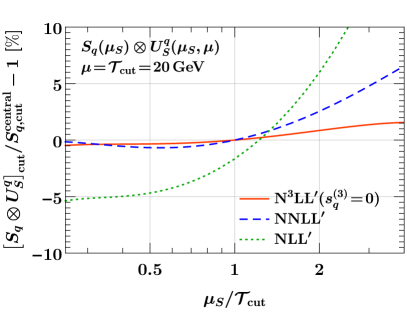
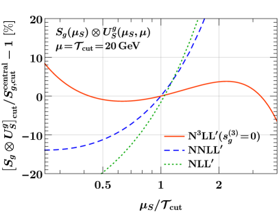
Figure -899: Residual scale dependence of the integrated resummed 𝒯0subscript𝒯0\mathcal{T}_{0} soft function for i=q𝑖𝑞i=q (left) and i=g𝑖𝑔i=g (right). Shown are the relative deviations from the NNLL result Si,cutcentralsuperscriptsubscript𝑆𝑖cutcentralS_{i,\mathrm{cut}}^{\mathrm{central}} at the central scale μS=𝒯cutsubscript𝜇𝑆subscript𝒯cut\mu_{S}=\mathcal{T}_{\mathrm{cut}}.

In figure -899, we take as an example 𝒯cut=μ=20GeVsubscript𝒯cut𝜇20GeV\mathcal{T}_{\mathrm{cut}}=\mu=20\,\mathrm{GeV} and show the residual μSsubscript𝜇𝑆\mu_{S} dependence of the resummed soft function when varying μSsubscript𝜇𝑆\mu_{S} around the canonical central value μS=𝒯cutsubscript𝜇𝑆subscript𝒯cut\mu_{S}=\mathcal{T}_{\mathrm{cut}} at NLL (dotted green), NNLL (dashed blue), and N3LL (solid orange). For the latter we set the currently unknown three-loop constant term si(3)=0superscriptsubscript𝑠𝑖30s_{i}^{(3)}=0. In all cases, we show the relative difference to the central value at NNLL. For simplicity we always use the same four-loop (N3LL) running for αssubscript𝛼𝑠\alpha_{s}, which formally amounts to a higher-order effect at (N)NLL. For the quark soft function (left panel), the μSsubscript𝜇𝑆\mu_{S} dependence is more than halved going from NLL to NNLL, and roughly halved again at N3LL. In the gluon case (right panel), the μSsubscript𝜇𝑆\mu_{S} dependence is noticeably larger, but also reduces significantly at each order as it should. Note that the missing three-loop constant term will add an additional source of μSsubscript𝜇𝑆\mu_{S} dependence due to its αs3(μS)superscriptsubscript𝛼𝑠3subscript𝜇𝑆\alpha_{s}^{3}(\mu_{S}) prefactor, which however should not change the general picture.

We stress that the residual μSsubscript𝜇𝑆\mu_{S} dependence in the resummed soft function by itself is not necessarily a good indicator of the perturbative uncertainty. Nevertheless, the reduction in the scale dependence still provides a useful cross check and an indication of the typical reduction of perturbative uncertainties one might expect at each order. We also emphasize that the size of the variations in figure -899 does not necessarily reflect the variations one should expect in the resummed cross section, where the evolution of the soft function happens in conjunction with the beam and hard functions.

2.3 𝒯0subscript𝒯0\mathcal{T}_{0} beam function

The beam function Bi(t,x,μ)subscript𝐵𝑖𝑡𝑥𝜇B_{i}(t,x,\mu) obeys the all-order RGE [49, 87]

μddμBi(t,x,μ)𝜇dd𝜇subscript𝐵𝑖𝑡𝑥𝜇\displaystyle\mu\frac{\mathrm{d}}{\mathrm{d}\mu}B_{i}(t,x,\mu) =dtγBi(tt,μ)Bi(t,x,μ),absentdifferential-dsuperscript𝑡superscriptsubscript𝛾𝐵𝑖𝑡superscript𝑡𝜇subscript𝐵𝑖superscript𝑡𝑥𝜇\displaystyle=\int\!\mathrm{d}t^{\prime}\,\gamma_{B}^{i}(t-t^{\prime},\mu)\,B_{i}(t^{\prime},x,\mu)\,,
γBi(t,μ)superscriptsubscript𝛾𝐵𝑖𝑡𝜇\displaystyle\gamma_{B}^{i}(t,\mu) =2Γcuspi[αs(μ)]0(t,μ2)+γBi[αs(μ)]δ(t),absent2superscriptsubscriptΓcusp𝑖delimited-[]subscript𝛼𝑠𝜇subscript0𝑡superscript𝜇2superscriptsubscript𝛾𝐵𝑖delimited-[]subscript𝛼𝑠𝜇𝛿𝑡\displaystyle=-2\Gamma_{\mathrm{cusp}}^{i}[\alpha_{s}(\mu)]\,\mathcal{L}_{0}(t,\mu^{2})+\gamma_{B}^{i}[\alpha_{s}(\mu)]\,\delta(t)\,, (2.15)

where Γcuspi(αs)superscriptsubscriptΓcusp𝑖subscript𝛼𝑠\Gamma_{\mathrm{cusp}}^{i}(\alpha_{s}) and γBi(αs)subscriptsuperscript𝛾𝑖𝐵subscript𝛼𝑠\gamma^{i}_{B}(\alpha_{s}) are the cusp and beam noncusp anomalous dimensions. For tΛQCDmuch-greater-than𝑡subscriptΛQCDt\gg\Lambda_{\mathrm{QCD}}, the beam function satisfies an OPE in terms of standard PDFs [49, 87]

Bi(t,x,μ)=jdzzij(t,z,μ)fj(xz,μ)[1+𝒪(ΛQCD2t)],subscript𝐵𝑖𝑡𝑥𝜇subscript𝑗d𝑧𝑧subscript𝑖𝑗𝑡𝑧𝜇subscript𝑓𝑗𝑥𝑧𝜇delimited-[]1𝒪superscriptsubscriptΛQCD2𝑡B_{i}(t,x,\mu)=\sum_{j}\int\!\frac{\mathrm{d}z}{z}\,\mathcal{I}_{ij}(t,z,\mu)\,f_{j}\Bigl{(}\frac{x}{z},\mu\Bigr{)}\,\biggl{[}1+\mathcal{O}\biggl{(}\frac{\Lambda_{\mathrm{QCD}}^{2}}{t}\biggr{)}\biggr{]}\,, (2.16)

where the ij(t,z,μ)subscript𝑖𝑗𝑡𝑧𝜇\mathcal{I}_{ij}(t,z,\mu) are perturbatively calculable matching coefficients. Taking into account the evolution of the PDFs, they obey the RGE [87]

μddμij(t,z,μ)=kdtdzzik(tt,zz,μ)[γBi(t,μ) 1kj(z)δ(t) 2Pkj(z,μ)],𝜇dd𝜇subscript𝑖𝑗𝑡𝑧𝜇subscript𝑘differential-dsuperscript𝑡dsuperscript𝑧superscript𝑧subscript𝑖𝑘𝑡superscript𝑡𝑧superscript𝑧𝜇delimited-[]superscriptsubscript𝛾𝐵𝑖superscript𝑡𝜇subscript1𝑘𝑗superscript𝑧𝛿superscript𝑡2subscript𝑃𝑘𝑗superscript𝑧𝜇\mu\frac{\mathrm{d}}{\mathrm{d}\mu}\mathcal{I}_{ij}(t,z,\mu)=\sum_{k}\int\!\mathrm{d}t^{\prime}\,\frac{\mathrm{d}z^{\prime}}{z^{\prime}}\,\mathcal{I}_{ik}\Bigl{(}t-t^{\prime},\frac{z}{z^{\prime}},\mu\Bigr{)}\Bigl{[}\gamma_{B}^{i}(t^{\prime},\mu)\,\mathbf{1}_{kj}(z^{\prime})-\delta(t^{\prime})\,2P_{kj}(z^{\prime},\mu)\Bigr{]}, (2.17)

where 𝟏ij(z)δijδ(1z)subscript1𝑖𝑗𝑧subscript𝛿𝑖𝑗𝛿1𝑧\mathbf{1}_{ij}(z)\equiv\delta_{ij}\,\delta(1-z) and 2Pij(z,μ)2subscript𝑃𝑖𝑗𝑧𝜇2P_{ij}(z,\mu) are the PDF anomalous dimensions.

By solving the RGE in eq. (2.17) recursively order by order, we can derive the complete structure of ij(t,z,μ)subscript𝑖𝑗𝑡𝑧𝜇\mathcal{I}_{ij}(t,z,\mu) at any given fixed order, as was done in refs. [88, 85] to NNLO. Following the same procedure as in section 2.2, keeping track of the flavor indices and Mellin convolutions, the (n+1)𝑛1(n+1)-loop term is determined from the up to n𝑛n-loop terms as

ij(n+1)(t,z,μ2)superscriptsubscript𝑖𝑗𝑛1𝑡𝑧superscript𝜇2\displaystyle\mathcal{I}_{ij}^{(n+1)}(t,z,\mu^{2}) =δ(t)Iij(n+1)(z)+t|+μ2dμ~2μ~2m=0n{Γnmi[0ij(m)(z)](t,μ~2)\displaystyle=\delta(t)\,I_{ij}^{(n+1)}(z)+\int_{t|_{+}}^{\mu^{2}}\!\frac{\mathrm{d}\tilde{\mu}^{2}}{\tilde{\mu}^{2}}\sum_{m=0}^{n}\biggl{\{}-\Gamma^{i}_{n-m}\bigl{[}\mathcal{L}_{0}\mathcal{I}^{(m)}_{ij}(z)\bigr{]}(t,\tilde{\mu}^{2}) (2.18)
+(mβnm+γBnmi2)ij(m)(t,z,μ~2)[(m)(t,μ~2)P(nm)]ij(z)},\displaystyle\quad+\Bigl{(}m\beta_{n-m}+\frac{\gamma_{B\,n-m}^{i}}{2}\Bigr{)}\mathcal{I}^{(m)}_{ij}(t,z,\tilde{\mu}^{2})-\bigl{[}\mathcal{I}^{(m)}(t,\tilde{\mu}^{2})P^{(n-m)}\bigr{]}_{ij}(z)\biggr{\}}\,,

where the μ𝜇\mu-independent boundary coefficients are defined as

ij(n)(t,z,μ2=t|+)=δ(t)Iij(n)(z).subscriptsuperscript𝑛𝑖𝑗𝑡𝑧superscript𝜇2evaluated-at𝑡𝛿𝑡subscriptsuperscript𝐼𝑛𝑖𝑗𝑧\mathcal{I}^{(n)}_{ij}(t,z,\mu^{2}=t|_{+})=\delta(t)\,I^{(n)}_{ij}(z)\,. (2.19)

Starting from the LO result, Iij(0)(z)=𝟏ij(z)δijδ(1z)subscriptsuperscript𝐼0𝑖𝑗𝑧subscript1𝑖𝑗𝑧subscript𝛿𝑖𝑗𝛿1𝑧I^{(0)}_{ij}(z)=\mathbf{1}_{ij}(z)\equiv\delta_{ij}\,\delta(1-z), we obtain up to two loops

ij(0)(t,z,μ2)superscriptsubscript𝑖𝑗0𝑡𝑧superscript𝜇2\displaystyle\mathcal{I}_{ij}^{(0)}(t,z,\mu^{2}) =δ(t) 1ij(z),absent𝛿𝑡subscript1𝑖𝑗𝑧\displaystyle=\delta(t)\,\mathbf{1}_{ij}(z)\,,
ij(1)(t,z,μ2)superscriptsubscript𝑖𝑗1𝑡𝑧superscript𝜇2\displaystyle\mathcal{I}_{ij}^{(1)}(t,z,\mu^{2}) =1(t,μ2)Γ0i 1ij(z)+0(t,μ2)[γB 0i2 1ij(z)+Pij(0)(z)]+δ(t)Iij(1)(z),absentsubscript1𝑡superscript𝜇2superscriptsubscriptΓ0𝑖subscript1𝑖𝑗𝑧subscript0𝑡superscript𝜇2delimited-[]superscriptsubscript𝛾𝐵 0𝑖2subscript1𝑖𝑗𝑧subscriptsuperscript𝑃0𝑖𝑗𝑧𝛿𝑡subscriptsuperscript𝐼1𝑖𝑗𝑧\displaystyle=\mathcal{L}_{1}(t,\mu^{2})\,\Gamma_{0}^{i}\,\mathbf{1}_{ij}(z)+\mathcal{L}_{0}(t,\mu^{2})\Bigl{[}-\frac{\gamma_{B\,0}^{i}}{2}\,\mathbf{1}_{ij}(z)+P^{(0)}_{ij}(z)\Bigr{]}+\delta(t)\,I^{(1)}_{ij}(z)\,,
ij(2)(t,z,μ2)superscriptsubscript𝑖𝑗2𝑡𝑧superscript𝜇2\displaystyle\mathcal{I}_{ij}^{(2)}(t,z,\mu^{2}) =3(t,μ2)(Γ0i)22 1ij(z)absentsubscript3𝑡superscript𝜇2superscriptsuperscriptsubscriptΓ0𝑖22subscript1𝑖𝑗𝑧\displaystyle=\mathcal{L}_{3}(t,\mu^{2})\,\frac{(\Gamma_{0}^{i})^{2}}{2}\,\mathbf{1}_{ij}(z)
+2(t,μ2)Γ0i2[(β0+32γB 0i)𝟏ij(z)+3Pij(0)(z)]subscript2𝑡superscript𝜇2superscriptsubscriptΓ0𝑖2delimited-[]subscript𝛽032superscriptsubscript𝛾𝐵 0𝑖subscript1𝑖𝑗𝑧3subscriptsuperscript𝑃0𝑖𝑗𝑧\displaystyle\quad+\mathcal{L}_{2}(t,\mu^{2})\,\frac{\Gamma_{0}^{i}}{2}\Bigl{[}-\Bigl{(}\beta_{0}+\frac{3}{2}\gamma_{B\,0}^{i}\Bigr{)}\mathbf{1}_{ij}(z)+3P^{(0)}_{ij}(z)\Bigr{]}
+1(t,μ2){[ζ2(Γ0i)2+(β0+γB 0i2)γB 0i2+Γ1i]𝟏ij(z)\displaystyle\quad+\mathcal{L}_{1}(t,\mu^{2})\biggl{\{}\Bigl{[}-\zeta_{2}(\Gamma_{0}^{i})^{2}+\Bigl{(}\beta_{0}+\frac{\gamma_{B\,0}^{i}}{2}\Bigr{)}\frac{\gamma_{B\,0}^{i}}{2}+\Gamma_{1}^{i}\Bigr{]}\mathbf{1}_{ij}(z)
(β0+γB 0i)Pij(0)(z)+(P(0)P(0))ij(z)+Γ0iIij(1)(z)}\displaystyle\qquad\qquad\qquad\quad-(\beta_{0}+\gamma_{B\,0}^{i})P^{(0)}_{ij}(z)+(P^{(0)}\!P^{(0)})_{ij}(z)+\Gamma_{0}^{i}\,I^{(1)}_{ij}(z)\biggr{\}}
+0(t,μ2){[Γ0i(ζ3Γ0i+ζ2γB 0i2)γB 1i2]𝟏ij(z)ζ2Γ0iPij(0)(z)\displaystyle\quad+\mathcal{L}_{0}(t,\mu^{2})\biggl{\{}\Bigl{[}\Gamma_{0}^{i}\Bigl{(}\zeta_{3}\Gamma_{0}^{i}+\zeta_{2}\frac{\gamma_{B\,0}^{i}}{2}\Bigr{)}-\frac{\gamma_{B\,1}^{i}}{2}\Bigr{]}\mathbf{1}_{ij}(z)-\zeta_{2}\Gamma_{0}^{i}\,P^{(0)}_{ij}(z)
+Pij(1)(z)(β0+γB 0i2)Iij(1)(z)+(I(1)P(0))ij(z)}\displaystyle\qquad\qquad\qquad\quad+P^{(1)}_{ij}(z)-\Bigl{(}\beta_{0}+\frac{\gamma_{B\,0}^{i}}{2}\Bigr{)}I^{(1)}_{ij}(z)+(I^{(1)}\!P^{(0)})_{ij}(z)\biggr{\}}
+δ(t)Iij(2)(z),𝛿𝑡subscriptsuperscript𝐼2𝑖𝑗𝑧\displaystyle\quad+\delta(t)\,I^{(2)}_{ij}(z)\,, (2.20)

which agrees with refs. [88, 85, 39]. The NLO and NNLO boundary coefficients Iij(1,2)(z)superscriptsubscript𝐼𝑖𝑗12𝑧I_{ij}^{(1,2)}(z) together with the required Mellin convolutions (P(0)P(0))ij(z)subscriptsuperscript𝑃0superscript𝑃0𝑖𝑗𝑧(P^{(0)}P^{(0)})_{ij}(z) and (I(1)P(0))ij(z)subscriptsuperscript𝐼1superscript𝑃0𝑖𝑗𝑧(I^{(1)}P^{(0)})_{ij}(z) can be found in refs. [85, 86].111We caution that the functions Pij(z)subscript𝑃𝑖𝑗𝑧P_{ij}(z) and Iij(z)subscript𝐼𝑖𝑗𝑧I_{ij}(z) in refs. [85, 86, 39] are expanded in powers of αs/(2π)subscript𝛼𝑠2𝜋\alpha_{s}/(2\pi) while here we expand them in powers of αs/(4π)subscript𝛼𝑠4𝜋\alpha_{s}/(4\pi).

Plugging eq. (2.3) back into eq. (2.18), we obtain the N3LO result

ij(3)(t,z,μ2)=δ(t)Iij(3)(z)+=05ij,(3)(z)(t,μ2)superscriptsubscript𝑖𝑗3𝑡𝑧superscript𝜇2𝛿𝑡superscriptsubscript𝐼𝑖𝑗3𝑧superscriptsubscript05superscriptsubscript𝑖𝑗3𝑧subscript𝑡superscript𝜇2\mathcal{I}_{ij}^{(3)}(t,z,\mu^{2})=\delta(t)\,I_{ij}^{(3)}(z)+\sum_{\ell=0}^{5}\mathcal{I}_{ij,\ell}^{(3)}(z)\,\mathcal{L}_{\ell}(t,\mu^{2}) (2.21)

with the coefficients

ij,5(3)(z)superscriptsubscript𝑖𝑗53𝑧\displaystyle\mathcal{I}_{ij,5}^{(3)}(z) =(Γ0i)38𝟏ij(z)absentsuperscriptsubscriptsuperscriptΓ𝑖038subscript1𝑖𝑗𝑧\displaystyle=\frac{(\Gamma^{i}_{0})^{3}}{8}\mathbf{1}_{ij}(z)
ij,4(3)(z)superscriptsubscript𝑖𝑗43𝑧\displaystyle\mathcal{I}_{ij,4}^{(3)}(z) =58(Γ0i)2[(23β0+γB 0i2)𝟏ij(z)+Pij(0)]absent58superscriptsubscriptsuperscriptΓ𝑖02delimited-[]23subscript𝛽0superscriptsubscript𝛾𝐵 0𝑖2subscript1𝑖𝑗𝑧superscriptsubscript𝑃𝑖𝑗0\displaystyle=\frac{5}{8}(\Gamma^{i}_{0})^{2}\Bigl{[}-\Bigl{(}\frac{2}{3}\beta_{0}+\frac{\gamma_{B\,0}^{i}}{2}\Bigr{)}\mathbf{1}_{ij}(z)+P_{ij}^{(0)}\Bigr{]}
ij,3(3)(z)superscriptsubscript𝑖𝑗33𝑧\displaystyle\mathcal{I}_{ij,3}^{(3)}(z) =Γ0i{[ζ2(Γ0i)2+β023+(53β0+γB 0i2)γB 0i2+Γ1i]𝟏ij(z)\displaystyle=\Gamma^{i}_{0}\biggl{\{}\Bigl{[}-\zeta_{2}(\Gamma^{i}_{0})^{2}+\frac{\beta_{0}^{2}}{3}+\Bigl{(}\frac{5}{3}\beta_{0}+\frac{\gamma_{B\,0}^{i}}{2}\Bigr{)}\frac{\gamma_{B\,0}^{i}}{2}+\Gamma_{1}^{i}\Bigr{]}\mathbf{1}_{ij}(z)
(53β0+γB 0i)Pij(0)(z)+(P(0)P(0))ij(z)+Γ0i2Iij(1)(z)}\displaystyle\quad-\Bigl{(}\frac{5}{3}\beta_{0}+\gamma_{B\,0}^{i}\Bigr{)}P_{ij}^{(0)}(z)+(P^{(0)}\!P^{(0)})_{ij}(z)+\frac{\Gamma_{0}^{i}}{2}I_{ij}^{(1)}(z)\biggr{\}}
ij,2(3)(z)superscriptsubscript𝑖𝑗23𝑧\displaystyle\mathcal{I}_{ij,2}^{(3)}(z) ={(Γ0i)2[52ζ3Γ0i+32ζ2(β0+γB 0i)](β0+34γB 0i)(β0γB 0i2+Γ1i)(γB 0i)316\displaystyle=\biggl{\{}(\Gamma^{i}_{0})^{2}\Bigl{[}\frac{5}{2}\zeta_{3}\Gamma^{i}_{0}+\frac{3}{2}\zeta_{2}(\beta_{0}+\gamma^{i}_{B\,0})\Bigr{]}-\Bigl{(}\beta_{0}+\frac{3}{4}\gamma^{i}_{B\,0}\Bigr{)}\Bigl{(}\beta_{0}\frac{\gamma^{i}_{B\,0}}{2}+\Gamma^{i}_{1}\Bigr{)}-\frac{(\gamma^{i}_{B\,0})^{3}}{16}
Γ0i2(β1+32γB 1i)}𝟏ij(z)+3[ζ2(Γ0i)2+β023+(β0+γB 0i4)γB 0i2+Γ1i2]Pij(0)(z)\displaystyle\quad-\frac{\Gamma^{i}_{0}}{2}\Bigl{(}\beta_{1}+\frac{3}{2}\gamma^{i}_{B\,1}\Bigr{)}\biggr{\}}\mathbf{1}_{ij}(z)+3\Bigl{[}-\zeta_{2}(\Gamma^{i}_{0})^{2}+\frac{\beta_{0}^{2}}{3}+\Bigl{(}\beta_{0}+\frac{\gamma^{i}_{B\,0}}{4}\Bigr{)}\frac{\gamma^{i}_{B\,0}}{2}+\frac{\Gamma^{i}_{1}}{2}\Bigr{]}P_{ij}^{(0)}(z)
32(β0+γB 0i2)(P(0)P(0))ij(z)+12(P(0)P(0)P(0))ij(z)32subscript𝛽0subscriptsuperscript𝛾𝑖𝐵 02subscriptsuperscript𝑃0superscript𝑃0𝑖𝑗𝑧12subscriptsuperscript𝑃0superscript𝑃0superscript𝑃0𝑖𝑗𝑧\displaystyle\quad-\frac{3}{2}\Bigl{(}\beta_{0}+\frac{\gamma^{i}_{B\,0}}{2}\Bigr{)}(P^{(0)}\!P^{(0)})_{ij}(z)+\frac{1}{2}(P^{(0)}\!P^{(0)}\!P^{(0)})_{ij}(z)
+32Γ0i[Pij(1)(z)(43β0+γB 0i2)Iij(1)(z)+(I(1)P(0))ij(z)]32subscriptsuperscriptΓ𝑖0delimited-[]superscriptsubscript𝑃𝑖𝑗1𝑧43subscript𝛽0subscriptsuperscript𝛾𝑖𝐵 02superscriptsubscript𝐼𝑖𝑗1𝑧subscriptsuperscript𝐼1superscript𝑃0𝑖𝑗𝑧\displaystyle\quad+\frac{3}{2}\Gamma^{i}_{0}\Bigl{[}P_{ij}^{(1)}(z)-\Bigl{(}\frac{4}{3}\beta_{0}+\frac{\gamma^{i}_{B\,0}}{2}\Bigr{)}I_{ij}^{(1)}(z)+(I^{(1)}\!P^{(0)})_{ij}(z)\Bigr{]}
ij,1(3)(z)superscriptsubscript𝑖𝑗13𝑧\displaystyle\mathcal{I}_{ij,1}^{(3)}(z) ={(Γ0i)2[ζ42Γ0i+ζ3(3β0+2γB 0i)]ζ2Γ0i[(3β0+γB 0i)γB 0i2+2Γ1i]\displaystyle=\biggl{\{}-(\Gamma^{i}_{0})^{2}\Bigl{[}\frac{\zeta_{4}}{2}\Gamma^{i}_{0}+\zeta_{3}(3\beta_{0}+2\gamma^{i}_{B\,0})\Bigr{]}-\zeta_{2}\Gamma^{i}_{0}\Bigl{[}(3\beta_{0}+\gamma^{i}_{B\,0})\frac{\gamma^{i}_{B\,0}}{2}+2\Gamma^{i}_{1}\Bigr{]}
+β0γB 1i+γB 0i2(β1+γB 1i)+Γ2i}𝟏ij(z)+{Γ0i[4ζ3Γ0i+ζ2(3β0+2γB 0i)]\displaystyle\quad+\beta_{0}\gamma^{i}_{B\,1}+\frac{\gamma^{i}_{B\,0}}{2}(\beta_{1}+\gamma^{i}_{B\,1})+\Gamma^{i}_{2}\biggr{\}}\mathbf{1}_{ij}(z)+\Bigl{\{}\Gamma^{i}_{0}\bigl{[}4\zeta_{3}\Gamma^{i}_{0}+\zeta_{2}(3\beta_{0}+2\gamma^{i}_{B\,0})\bigr{]}
(β1+γB 1i)}P(0)ij(z)2ζ2Γi0(P(0)P(0))ij(z)(2β0+γB 0i)P(1)ij(z)\displaystyle\quad-(\beta_{1}+\gamma^{i}_{B\,1})\Bigr{\}}P^{(0)}_{ij}(z)-2\zeta_{2}\Gamma^{i}_{0}(P^{(0)}\!P^{(0)})_{ij}(z)-(2\beta_{0}+\gamma^{i}_{B\,0})P^{(1)}_{ij}(z)
+(P(0)P(1)+P(1)P(0))ij(z)+[ζ2(Γ0i)2+2β02+(3β0+γB 0i2)γB 0i2+Γ1i]Iij(1)(z)subscriptsuperscript𝑃0superscript𝑃1superscript𝑃1superscript𝑃0𝑖𝑗𝑧delimited-[]subscript𝜁2superscriptsubscriptsuperscriptΓ𝑖022superscriptsubscript𝛽023subscript𝛽0subscriptsuperscript𝛾𝑖𝐵 02subscriptsuperscript𝛾𝑖𝐵 02subscriptsuperscriptΓ𝑖1subscriptsuperscript𝐼1𝑖𝑗𝑧\displaystyle\quad+(P^{(0)}\!P^{(1)}\!+\!P^{(1)}\!P^{(0)})_{ij}(z)+\Bigl{[}-\zeta_{2}(\Gamma^{i}_{0})^{2}+2\beta_{0}^{2}+\Bigl{(}3\beta_{0}+\frac{\gamma^{i}_{B\,0}}{2}\Bigr{)}\frac{\gamma^{i}_{B\,0}}{2}+\Gamma^{i}_{1}\Bigr{]}I^{(1)}_{ij}(z)
(3β0+γB 0i)(I(1)P(0))ij(z)+(I(1)P(0)P(0))ij(z)+Γ0iIij(2)(z)3subscript𝛽0subscriptsuperscript𝛾𝑖𝐵 0subscriptsuperscript𝐼1superscript𝑃0𝑖𝑗𝑧subscriptsuperscript𝐼1superscript𝑃0superscript𝑃0𝑖𝑗𝑧subscriptsuperscriptΓ𝑖0subscriptsuperscript𝐼2𝑖𝑗𝑧\displaystyle\quad-(3\beta_{0}+\gamma^{i}_{B\,0})(I^{(1)}\!P^{(0)})_{ij}(z)+(I^{(1)}\!P^{(0)}\!P^{(0)})_{ij}(z)+\Gamma^{i}_{0}\,I^{(2)}_{ij}(z)
ij,0(3)(z)superscriptsubscript𝑖𝑗03𝑧\displaystyle\mathcal{I}_{ij,0}^{(3)}(z) ={(Γ0i)2[Γ0i(2ζ2ζ33ζ5)+ζ4(β0+γB 0i4)]+ζ3Γ0i[(β0+γB 0i2)γB 0i2+2Γ1i]\displaystyle=\biggl{\{}(\Gamma^{i}_{0})^{2}\Bigl{[}-\Gamma^{i}_{0}(2\zeta_{2}\zeta_{3}-3\zeta_{5})+\zeta_{4}\Bigl{(}\beta_{0}+\frac{\gamma^{i}_{B\,0}}{4}\Bigr{)}\Bigr{]}+\zeta_{3}\Gamma^{i}_{0}\Bigl{[}\Bigl{(}\beta_{0}+\frac{\gamma^{i}_{B\,0}}{2}\Bigr{)}\frac{\gamma^{i}_{B\,0}}{2}+2\Gamma^{i}_{1}\Bigr{]}
+ζ22(γB 0iΓ1i+Γ0iγB 1i)γB 2i2}𝟏ij(z){Γ0i[ζ42Γ0i+ζ3(β0+γB 0i)]\displaystyle\quad+\frac{\zeta_{2}}{2}\bigl{(}\gamma^{i}_{B\,0}\Gamma^{i}_{1}+\Gamma^{i}_{0}\gamma^{i}_{B\,1}\bigr{)}-\frac{\gamma^{i}_{B\,2}}{2}\biggr{\}}\mathbf{1}_{ij}(z)-\biggl{\{}\Gamma^{i}_{0}\Bigl{[}\frac{\zeta_{4}}{2}\Gamma^{i}_{0}+\zeta_{3}(\beta_{0}+\gamma^{i}_{B\,0})\Bigr{]}
+ζ2Γ1i}P(0)ij(z)+Γi0[ζ3(P(0)P(0))ij(z)ζ2Pij(1)(z)]+P(2)ij(z)\displaystyle\quad+\zeta_{2}\Gamma^{i}_{1}\biggr{\}}P^{(0)}_{ij}(z)+\Gamma^{i}_{0}\bigl{[}\zeta_{3}(P^{(0)}\!P^{(0)})_{ij}(z)-\zeta_{2}P^{(1)}_{ij}(z)\bigr{]}+P^{(2)}_{ij}(z)
+{Γ0i[ζ3Γ0i+ζ2(β0+γB 0i2)](β1+γB 1i2)}Iij(1)(z)Γ0iζ2(I(1)P(0))ij(z)subscriptsuperscriptΓ𝑖0delimited-[]subscript𝜁3subscriptsuperscriptΓ𝑖0subscript𝜁2subscript𝛽0subscriptsuperscript𝛾𝑖𝐵 02subscript𝛽1subscriptsuperscript𝛾𝑖𝐵12subscriptsuperscript𝐼1𝑖𝑗𝑧subscriptsuperscriptΓ𝑖0subscript𝜁2subscriptsuperscript𝐼1superscript𝑃0𝑖𝑗𝑧\displaystyle\quad+\biggl{\{}\Gamma^{i}_{0}\Bigl{[}\zeta_{3}\Gamma^{i}_{0}+\zeta_{2}\Bigl{(}\beta_{0}+\frac{\gamma^{i}_{B\,0}}{2}\Bigr{)}\Bigr{]}-\Bigl{(}\beta_{1}+\frac{\gamma^{i}_{B\,1}}{2}\Bigr{)}\biggr{\}}I^{(1)}_{ij}(z)-\Gamma^{i}_{0}\zeta_{2}(I^{(1)}\!P^{(0)})_{ij}(z)
+(I(1)P(1))ij(z)(2β0+γB 0i2)Iij(2)(z)+(I(2)P(0))ij(z).subscriptsuperscript𝐼1superscript𝑃1𝑖𝑗𝑧2subscript𝛽0subscriptsuperscript𝛾𝑖𝐵 02subscriptsuperscript𝐼2𝑖𝑗𝑧subscriptsuperscript𝐼2superscript𝑃0𝑖𝑗𝑧\displaystyle\quad+(I^{(1)}\!P^{(1)})_{ij}(z)-\Bigl{(}2\beta_{0}+\frac{\gamma^{i}_{B\,0}}{2}\Bigr{)}I^{(2)}_{ij}(z)+(I^{(2)}\!P^{(0)})_{ij}(z)\,. (2.22)

The required anomalous dimensions and splitting functions up to three loops are given in appendix D. We have evaluated all Mellin convolutions appearing in eq. (2.3) using the MT package [108]. To calculate (I(2)P(0))ij(z)subscriptsuperscript𝐼2superscript𝑃0𝑖𝑗𝑧(I^{(2)}P^{(0)})_{ij}(z) this required employing the identity

Li3(11+z)+Li3(z)+Li3(z1+z)=ζ3ζ2ln(1+z)12ln2(1+z)lnz+13ln3(1+z).subscriptLi311𝑧subscriptLi3𝑧subscriptLi3𝑧1𝑧subscript𝜁3subscript𝜁21𝑧12superscript21𝑧𝑧13superscript31𝑧\mathrm{Li}_{3}\Bigl{(}\frac{1}{1+z}\Bigr{)}+\mathrm{Li}_{3}(-z)+\mathrm{Li}_{3}\Bigl{(}\frac{z}{1+z}\Bigr{)}=\zeta_{3}-\zeta_{2}\ln(1+z)-\frac{1}{2}\ln^{2}(1+z)\ln z+\frac{1}{3}\ln^{3}(1+z)\,. (2.23)

Numerical impact

As for the soft function above, to illustrate the numerical impact of the three-loop corrections, we consider the integrated resummed beam function

(BiUBi)cut(tcut,x,μ)subscripttensor-productsubscript𝐵𝑖superscriptsubscript𝑈𝐵𝑖cutsubscript𝑡cut𝑥𝜇\displaystyle(B_{i}\otimes U_{B}^{i})_{\mathrm{cut}}(t_{\mathrm{cut}},x,\mu) =tcutdtdtBi(t,x,μB)UBi(tt,μB,μ).absentsuperscriptsubscript𝑡cutdifferential-d𝑡differential-dsuperscript𝑡subscript𝐵𝑖𝑡𝑥subscript𝜇𝐵superscriptsubscript𝑈𝐵𝑖𝑡superscript𝑡subscript𝜇𝐵𝜇\displaystyle=\int^{t_{\mathrm{cut}}}\!\mathrm{d}t\,\int\!\mathrm{d}t^{\prime}\,B_{i}(t,x,\mu_{B})\,U_{B}^{i}(t-t^{\prime},\mu_{B},\mu)\,. (2.24)

The explicit expression for the beam function evolution kernel UBi(t,μB,μ)superscriptsubscript𝑈𝐵𝑖𝑡subscript𝜇𝐵𝜇U_{B}^{i}(t,\mu_{B},\mu) can be found in refs. [87, 88].

Refer to caption
Refer to caption
Refer to caption
Refer to caption
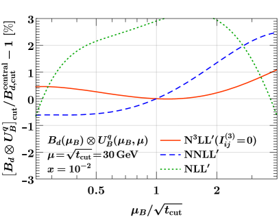
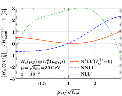
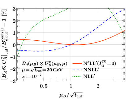
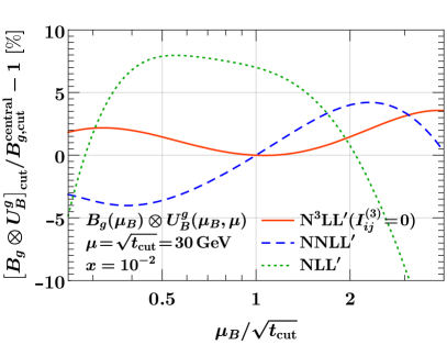
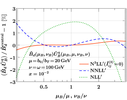
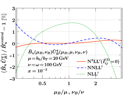
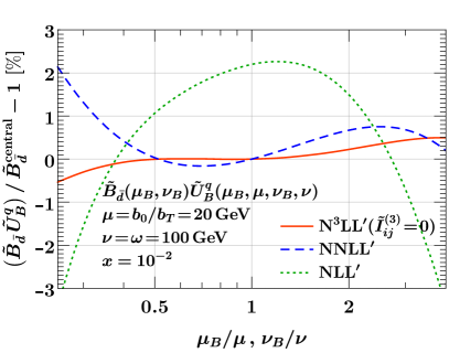
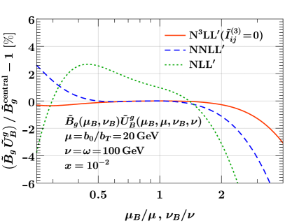
Figure -898: Residual scale dependence of the resummed integrated 𝒯Nsubscript𝒯𝑁\mathcal{T}_{N} beam function for i=d𝑖𝑑i=d (top left), u𝑢u (top right), d¯¯𝑑\bar{d} (bottom left), and g𝑔g (bottom right). Shown are the relative deviations from the NNLL result Bi,cutcentralsuperscriptsubscript𝐵𝑖cutcentralB_{i,\mathrm{cut}}^{\mathrm{central}} at the central scale μB=tcutsubscript𝜇𝐵subscript𝑡cut\mu_{B}=\sqrt{t_{\mathrm{cut}}}.

In figure -898, we show the residual μBsubscript𝜇𝐵\mu_{B} dependence of the resummed integrated beam function at fixed representative values of x=102𝑥superscript102x=10^{-2} and tcut=μ=30GeVsubscript𝑡cut𝜇30GeV\sqrt{t_{\mathrm{cut}}}=\mu=30\,\mathrm{GeV}. We again show the relative difference to the NNLL central result at μB=tcutsubscript𝜇𝐵subscript𝑡cut\mu_{B}=\sqrt{t_{\mathrm{cut}}} at NLL (dotted green), NNLL (dashed blue), and N3LL with the unknown three-loop Iij(3)(z)=0superscriptsubscript𝐼𝑖𝑗3𝑧0I_{ij}^{(3)}(z)=0 (solid orange). We use the MMHT2014nnlo68cl [109] NNLO PDFs and four-loop running of αssubscript𝛼𝑠\alpha_{s} everywhere. These evolution orders are sufficient to ensure the formal cancellation of the μBsubscript𝜇𝐵\mu_{B} dependence at N3LL, while at lower orders they amount to a higher-order effect. Numerical results to N3LL with PDFs and αssubscript𝛼𝑠\alpha_{s} evolution at corresponding lower orders can be found in ref. [86]. The residual dependence on μBsubscript𝜇𝐵\mu_{B} is noticeably reduced by about a factor of two at N3LL compared to NNLL. The missing three-loop constant terms will again add an additional source of μBsubscript𝜇𝐵\mu_{B} dependence due to its αs3(μB)superscriptsubscript𝛼𝑠3subscript𝜇𝐵\alpha_{s}^{3}(\mu_{B}) prefactor and also the scale dependence of the PDFs, which however should not change the qualitative picture.

2.4 Beam function coefficients in the eikonal limit

We now obtain the beam function coefficients Iij(n)(z)superscriptsubscript𝐼𝑖𝑗𝑛𝑧I_{ij}^{(n)}(z) in the z1𝑧1z\to 1 limit. As was already pointed out and exploited in the NNLO calculation in refs. [85, 86], the beam function in this limit is effectively determined by a matrix element of eikonal Wilson lines. Here, we exploit a recently derived consistency relation [97] that explicitly relates the Iij(n)(z1)superscriptsubscript𝐼𝑖𝑗𝑛𝑧1I_{ij}^{(n)}(z\to 1) to the threshold soft function to all orders in αssubscript𝛼𝑠\alpha_{s}. Consistency relations of this kind generically arise from different factorization theorems that apply in different limits of the same multi-differential cross section. In particular, a soft or collinear matrix element of several arguments will refactorize into a product (or convolution) of simpler pieces of fewer arguments by taking a stronger limit.

We start by defining the color-singlet lightcone momenta qsuperscript𝑞minus-or-plusq^{\mp} and corresponding momentum fractions xsubscript𝑥minus-or-plusx_{\mp},

qn¯q=Q2+qT2e+Y,q+nq=Q2+qT2eY,x=qEcm.formulae-sequencesuperscript𝑞¯𝑛𝑞superscript𝑄2superscriptsubscript𝑞𝑇2superscript𝑒𝑌superscript𝑞𝑛𝑞superscript𝑄2superscriptsubscript𝑞𝑇2superscript𝑒𝑌subscript𝑥minus-or-plussuperscript𝑞minus-or-plussubscript𝐸cmq^{-}\equiv{\bar{n}}\cdot q=\sqrt{Q^{2}+q_{T}^{2}}\,e^{+Y}\,,\qquad q^{+}\equiv n\cdot q=\sqrt{Q^{2}+q_{T}^{2}}\,e^{-Y}\,,\qquad x_{\mp}=\frac{q^{\mp}}{E_{\mathrm{cm}}}\,. (2.25)

As recently shown in ref. [97], in the generalized threshold limit x1subscript𝑥1x_{-}\to 1 but generic x+subscript𝑥x_{+}, the inclusive color-singlet cross section differential in q±superscript𝑞plus-or-minusq^{\pm} factorizes as

dσdqdq+=a,bHab(q+q,μ)dtfathr[x(1+tq+q),μ]Bb(t,x+,μ)[1+𝒪(1x)].d𝜎dsuperscript𝑞dsuperscript𝑞subscript𝑎𝑏subscript𝐻𝑎𝑏superscript𝑞superscript𝑞𝜇differential-d𝑡superscriptsubscript𝑓𝑎thrsubscript𝑥1𝑡superscript𝑞superscript𝑞𝜇subscript𝐵𝑏𝑡subscript𝑥𝜇delimited-[]1𝒪1subscript𝑥\frac{\mathrm{d}\sigma}{\mathrm{d}q^{-}\mathrm{d}q^{+}}=\sum_{a,b}H_{ab}(q^{+}q^{-},\mu)\int\!\mathrm{d}t\,f_{a}^{\mathrm{thr}}\Bigl{[}x_{-}\Bigl{(}1+\frac{t}{q^{+}q^{-}}\Bigr{)},\mu\Bigr{]}B_{b}(t,x_{+},\mu)\,\bigl{[}1+\mathcal{O}(1-x_{-})\bigr{]}\,. (2.26)

Here, Habsubscript𝐻𝑎𝑏H_{ab} is the same hard function as in eq. (2.1), and Bbsubscript𝐵𝑏B_{b} is the same inclusive beam function as in eq. (2.1). The threshold PDF fathr(x)subscriptsuperscript𝑓thr𝑎𝑥f^{\mathrm{thr}}_{a}(x) encodes the extraction of parton a𝑎a from the proton for x1𝑥1x\to 1.

On the other hand, in the well-known and stronger soft threshold limit, where both x1subscript𝑥1x_{-}\to 1 and x+1subscript𝑥1x_{+}\to 1, the cross section factorizes as [110, 111, 112, 113, 114]

dσdqdq+d𝜎dsuperscript𝑞dsuperscript𝑞\displaystyle\frac{\mathrm{d}\sigma}{\mathrm{d}q^{-}\mathrm{d}q^{+}} =a,bHab(q+q,μ)dkdk+fathr[x(1+kq),μ]fbthr[x+(1+k+q+),μ]absentsubscript𝑎𝑏subscript𝐻𝑎𝑏superscript𝑞superscript𝑞𝜇differential-dsuperscript𝑘differential-dsuperscript𝑘subscriptsuperscript𝑓thr𝑎subscript𝑥1superscript𝑘superscript𝑞𝜇subscriptsuperscript𝑓thr𝑏subscript𝑥1superscript𝑘superscript𝑞𝜇\displaystyle=\sum_{a,b}H_{ab}(q^{+}q^{-},\mu)\int\!\mathrm{d}k^{-}\mathrm{d}k^{+}\,f^{\mathrm{thr}}_{a}\Bigl{[}x_{-}\Bigl{(}1+\frac{k^{-}}{q^{-}}\Bigr{)},\mu\Bigr{]}\,f^{\mathrm{thr}}_{b}\Bigl{[}x_{+}\Bigl{(}1+\frac{k^{+}}{q^{+}}\Bigr{)},\mu\Bigr{]}
×Sithr(k,k+,μ)[1+𝒪(1x,1x+)].absentsubscriptsuperscript𝑆thr𝑖superscript𝑘superscript𝑘𝜇delimited-[]1𝒪1subscript𝑥1subscript𝑥\displaystyle\quad\times S^{\mathrm{thr}}_{i}(k^{-},k^{+},\mu)\,\bigl{[}1+\mathcal{O}(1-x_{-},1-x_{+})\bigr{]}\,. (2.27)

The new ingredient is the threshold soft function Sithr(k,k+,μ)subscriptsuperscript𝑆thr𝑖superscript𝑘superscript𝑘𝜇S^{\mathrm{thr}}_{i}(k^{-},k^{+},\mu). It describes the process-independent contribution of soft emissions with total lightcone momenta k+=nksuperscript𝑘𝑛𝑘k^{+}=n\cdot k and k=n¯ksuperscript𝑘¯𝑛𝑘k^{-}={\bar{n}}\cdot k. It also only depends on the color representation ci={q,g}𝑐𝑖𝑞𝑔c\equiv i=\{q,g\} of the incoming partons.

The threshold soft function is defined as a vacuum matrix element of Wilson lines that are invariant under longitudinal boosts, and therefore satisfies the rescaling property

Sithr(k,k+,μ)=Sithr(e+yk,eyk+,μ).subscriptsuperscript𝑆thr𝑖superscript𝑘superscript𝑘𝜇subscriptsuperscript𝑆thr𝑖superscript𝑒𝑦superscript𝑘superscript𝑒𝑦superscript𝑘𝜇\displaystyle S^{\mathrm{thr}}_{i}(k^{-},k^{+},\mu)=S^{\mathrm{thr}}_{i}(e^{+y}k^{-},e^{-y}k^{+},\mu)\,. (2.28)

More specifically, in the context of SCET, the soft function is invariant under RPI-III transformations [115, 116]. Exploiting this property, the soft function can be extracted [111, 14, 117, 82, 19] from the soft-virtual limit of the total color-singlet production cross section dσ/dQ2d𝜎dsuperscript𝑄2\mathrm{d}\sigma/\mathrm{d}Q^{2}, which is known to 𝒪(αs3)𝒪superscriptsubscript𝛼𝑠3\mathcal{O}(\alpha_{s}^{3}) [11, 12]. In appendix B, we review this procedure and give explicit results for Sithr(k,k+,μ)subscriptsuperscript𝑆thr𝑖superscript𝑘superscript𝑘𝜇S^{\mathrm{thr}}_{i}(k^{-},k^{+},\mu) to three loops.

The factorization theorems eqs. (2.26) and (2.4) describe the same cross section and share a number of common ingredients. In particular, only the beam function depends on x+subscript𝑥x_{+} in eq. (2.26). Further expanding eq. (2.26) in the limit x=x+1𝑥subscript𝑥1x=x_{+}\to 1, it must reproduce eq. (2.4). As a result, the eikonal x1𝑥1x\to 1 limit of the beam function must coincide with the threshold soft function [97],

Bi(t,x,μ)=dkωSithr(tω,k,μ)fithr[x(1+kω),μ][1+𝒪(1x)].subscript𝐵𝑖𝑡𝑥𝜇d𝑘𝜔subscriptsuperscript𝑆thr𝑖𝑡𝜔𝑘𝜇superscriptsubscript𝑓𝑖thr𝑥1𝑘𝜔𝜇delimited-[]1𝒪1𝑥B_{i}(t,x,\mu)=\int\!\frac{\mathrm{d}k}{\omega}\,S^{\mathrm{thr}}_{i}\Bigl{(}\frac{t}{\omega},k,\mu\Bigr{)}\,f_{i}^{\mathrm{thr}}\Bigl{[}x\Bigl{(}1+\frac{k}{\omega}\Bigr{)},\mu\Bigr{]}\,\bigl{[}1+\mathcal{O}(1-x)\bigr{]}\,. (2.29)

Replacing fithr[x(1+1z)]subscriptsuperscript𝑓thr𝑖delimited-[]𝑥11𝑧f^{\mathrm{thr}}_{i}[x(1+1-z)] by fi(x/z)/zsubscript𝑓𝑖𝑥𝑧𝑧f_{i}(x/z)/z, which is justified at leading power in 1z1𝑧1-z, yields the corresponding relation for the matching coefficients [97],

ij(t,z,μ)=δijSithr[tω,ω(1z),μ][1+𝒪(1z)].subscript𝑖𝑗𝑡𝑧𝜇subscript𝛿𝑖𝑗superscriptsubscript𝑆𝑖thr𝑡𝜔𝜔1𝑧𝜇delimited-[]1𝒪1𝑧\mathcal{I}_{ij}(t,z,\mu)=\delta_{ij}\,S_{i}^{\mathrm{thr}}\Bigl{[}\frac{t}{\omega},\omega(1-z),\mu\Bigr{]}\,\bigl{[}1+\mathcal{O}(1-z)\bigr{]}\,. (2.30)

This relation captures all terms in ij(t,z,μ)subscript𝑖𝑗𝑡𝑧𝜇\mathcal{I}_{ij}(t,z,\mu) that are singular for z1𝑧1z\to 1, while power corrections have at most an integrable singularity for z1𝑧1z\to 1. Notably, the beam function becomes flavor diagonal as z1𝑧1z\to 1, while offdiagonal channels are 𝒪(1z)𝒪1𝑧\mathcal{O}(1-z) suppressed. By eq. (2.30), the matching coefficients also inherit the rescaling property in eq. (2.28), i.e., in the limit z1𝑧1z\to 1, they become invariant under a simultaneous rescaling te+ytmaps-to𝑡superscript𝑒𝑦𝑡t\mapsto e^{+y}t and 1zey(1z)maps-to1𝑧superscript𝑒𝑦1𝑧1-z\mapsto e^{-y}(1-z). In other words, they are symmetric in t/ω𝑡𝜔t/\omega and ω(1z)𝜔1𝑧\omega(1-z) such that the dependence on ω𝜔\omega cancels on the right-hand side.

In ref. [97], eq. (2.30) was explicitly confirmed at two loops by comparison to refs. [85, 86]. We now use it to predict the beam function coefficients in the eikonal limit at three loops. They are given by the coefficient of δ(k)𝛿superscript𝑘\delta(k^{-}) in the threshold soft function upon identifying δ(k+)δ(1z)maps-to𝛿superscript𝑘𝛿1𝑧\delta(k^{+})\mapsto\delta(1-z) and n(k+,μ)n(1z)maps-tosubscript𝑛superscript𝑘𝜇subscript𝑛1𝑧\mathcal{L}_{n}(k^{+},\mu)\mapsto\mathcal{L}_{n}(1-z). Including the one-loop and two-loop results for reference, we find

Iij(1)(z)superscriptsubscript𝐼𝑖𝑗1𝑧\displaystyle I_{ij}^{(1)}(z) =δij[1(1z)Γ0i+δ(1z)sithr(1)]+𝒪[(1z)0],absentsubscript𝛿𝑖𝑗delimited-[]subscript11𝑧superscriptsubscriptΓ0𝑖𝛿1𝑧subscriptsuperscript𝑠thr1𝑖𝒪delimited-[]superscript1𝑧0\displaystyle=\delta_{ij}\Bigl{[}\mathcal{L}_{1}(1-z)\,\Gamma_{0}^{i}+\delta(1-z)\,s^{\mathrm{thr}{(1)}}_{i}\Bigr{]}+\mathcal{O}\bigl{[}(1-z)^{0}\bigr{]}\,,
Iij(2)(z)superscriptsubscript𝐼𝑖𝑗2𝑧\displaystyle I_{ij}^{(2)}(z) =δij{3(1z)(Γ0i)222(1z)Γ0i2β0+1(1z)[2ζ2(Γ0i)2+Γ1i+Γ0isithr(1)]\displaystyle=\delta_{ij}\biggl{\{}\mathcal{L}_{3}(1-z)\,\frac{(\Gamma_{0}^{i})^{2}}{2}-\mathcal{L}_{2}(1-z)\,\frac{\Gamma_{0}^{i}}{2}\beta_{0}+\mathcal{L}_{1}(1-z)\Bigl{[}-2\zeta_{2}(\Gamma_{0}^{i})^{2}+\Gamma_{1}^{i}+\Gamma_{0}^{i}\,s^{\mathrm{thr}{(1)}}_{i}\Bigr{]}
+0(1z)[2ζ3(Γ0i)2+γS 1i2β0sithr(1)]+δ(1z)sithr(2)}+𝒪[(1z)0],\displaystyle\quad\qquad+\mathcal{L}_{0}(1-z)\Bigl{[}2\zeta_{3}(\Gamma_{0}^{i})^{2}+\frac{\gamma_{S\,1}^{i}}{2}-\beta_{0}\,s^{\mathrm{thr}{(1)}}_{i}\Bigr{]}+\delta(1-z)\,s^{\mathrm{thr}{(2)}}_{i}\biggr{\}}+\mathcal{O}\bigl{[}(1-z)^{0}\bigr{]}\,,
Iij(3)(z)superscriptsubscript𝐼𝑖𝑗3𝑧\displaystyle I_{ij}^{(3)}(z) =δij{5(1z)(Γ0i)384(1z)512(Γ0i)2β0\displaystyle=\delta_{ij}\biggl{\{}\mathcal{L}_{5}(1-z)\,\frac{(\Gamma^{i}_{0})^{3}}{8}-\mathcal{L}_{4}(1-z)\,\frac{5}{12}(\Gamma^{i}_{0})^{2}\beta_{0}
+3(1z)Γ0i[2ζ2(Γ0i)2+β023+Γ1i+Γ0i2sithr(1)]subscript31𝑧subscriptsuperscriptΓ𝑖0delimited-[]2subscript𝜁2superscriptsubscriptsuperscriptΓ𝑖02superscriptsubscript𝛽023superscriptsubscriptΓ1𝑖superscriptsubscriptΓ0𝑖2superscriptsubscript𝑠𝑖thr1\displaystyle\quad\qquad+\mathcal{L}_{3}(1-z)\,\Gamma^{i}_{0}\Bigl{[}-2\zeta_{2}(\Gamma^{i}_{0})^{2}+\frac{\beta_{0}^{2}}{3}+\Gamma_{1}^{i}+\frac{\Gamma_{0}^{i}}{2}s_{i}^{\mathrm{thr}{(1)}}\Bigr{]}
+2(1z)[(Γ0i)2(5ζ3Γ0i+3ζ2β0)β0Γ1iΓ0i2(β132γS 1i+4β0sithr(1))]subscript21𝑧delimited-[]superscriptsubscriptsuperscriptΓ𝑖025subscript𝜁3subscriptsuperscriptΓ𝑖03subscript𝜁2subscript𝛽0subscript𝛽0subscriptsuperscriptΓ𝑖1subscriptsuperscriptΓ𝑖02subscript𝛽132subscriptsuperscript𝛾𝑖𝑆14subscript𝛽0superscriptsubscript𝑠𝑖thr1\displaystyle\quad\qquad+\mathcal{L}_{2}(1-z)\,\Bigl{[}(\Gamma^{i}_{0})^{2}(5\zeta_{3}\Gamma^{i}_{0}+3\zeta_{2}\beta_{0})-\beta_{0}\Gamma^{i}_{1}-\frac{\Gamma^{i}_{0}}{2}\Bigl{(}\beta_{1}-\frac{3}{2}\gamma^{i}_{S\,1}+4\beta_{0}\,s_{i}^{\mathrm{thr}{(1)}}\Bigr{)}\Bigr{]}
+1(1z)[(Γ0i)2(4ζ4Γ0i6ζ3β0)4ζ2Γ0iΓ1iβ0γS 1i+Γ2i\displaystyle\quad\qquad+\mathcal{L}_{1}(1-z)\,\Bigl{[}(\Gamma^{i}_{0})^{2}(4\zeta_{4}\Gamma^{i}_{0}-6\zeta_{3}\beta_{0})-4\zeta_{2}\Gamma^{i}_{0}\Gamma^{i}_{1}-\beta_{0}\gamma^{i}_{S\,1}+\Gamma^{i}_{2}
+(2ζ2(Γ0i)2+2β02+Γ1i)sithr(1)+Γ0isithr(2)]\displaystyle\quad\qquad\hskip 55.97205pt+\bigl{(}-2\zeta_{2}(\Gamma^{i}_{0})^{2}+2\beta_{0}^{2}+\Gamma^{i}_{1}\bigr{)}s_{i}^{\mathrm{thr}{(1)}}+\Gamma^{i}_{0}\,s_{i}^{\mathrm{thr}{(2)}}\Bigr{]}
+0(1z)[(Γ0i)2(Γ0i(8ζ2ζ36ζ5)+2ζ4β0)+Γ0i(4ζ3Γ1iζ2γS 1i)+γS 2i2\displaystyle\quad\qquad+\mathcal{L}_{0}(1-z)\,\Bigl{[}(\Gamma^{i}_{0})^{2}\bigl{(}-\Gamma^{i}_{0}(8\zeta_{2}\zeta_{3}-6\zeta_{5})+2\zeta_{4}\beta_{0}\bigr{)}+\Gamma^{i}_{0}(4\zeta_{3}\Gamma^{i}_{1}-\zeta_{2}\gamma^{i}_{S\,1})+\frac{\gamma^{i}_{S\,2}}{2}
+((Γ0i)22ζ3+Γ0i2ζ2β0β1+γS 1i2)sithr(1)2β0sithr(2)]\displaystyle\quad\qquad\hskip 55.97205pt+\Bigl{(}(\Gamma^{i}_{0})^{2}2\zeta_{3}+\Gamma^{i}_{0}2\zeta_{2}\beta_{0}-\beta_{1}+\frac{\gamma^{i}_{S\,1}}{2}\Bigr{)}s_{i}^{\mathrm{thr}{(1)}}-2\beta_{0}\,s_{i}^{\mathrm{thr}{(2)}}\Bigr{]}
+δ(1z)sithr(3)}+𝒪[(1z)0].\displaystyle\quad\qquad+\delta(1-z)\,s^{\mathrm{thr}{(3)}}_{i}\biggr{\}}+\mathcal{O}\bigl{[}(1-z)^{0}\bigr{]}\,. (2.31)

The boundary coefficients sithr(n)subscriptsuperscript𝑠thr𝑛𝑖s^{\mathrm{thr}(n)}_{i} of the threshold soft function are given in eq. (B.2). We have exploited that the noncusp anomalous dimension of the threshold soft function is given by γSi(αs)superscriptsubscript𝛾𝑆𝑖subscript𝛼𝑠-\gamma_{S}^{i}(\alpha_{s}), see appendix B.2. For brevity, we also used that γS 0i=0superscriptsubscript𝛾𝑆 0𝑖0\gamma_{S\,0}^{i}=0. The result for generic γS 0isuperscriptsubscript𝛾𝑆 0𝑖\gamma_{S\,0}^{i} can be read off from the full expression for the threshold soft function in eq. (B.2).

The three-loop result in eq. (2.4) is new and a genuine prediction of the consistency relation in eq. (2.30). We stress that the information provided by it goes beyond the RGE predicted three-loop structure in eq. (2.3). The fact that the leading z1𝑧1z\to 1 terms must be symmetric in t/ω𝑡𝜔t/\omega and ω(1z)𝜔1𝑧\omega(1-z) allows one to directly determine (or check) the δ(t)n(1z)𝛿𝑡subscript𝑛1𝑧\delta(t)\mathcal{L}_{n}(1-z) terms from the RGE-predicted n(t)δ(1z)subscript𝑛𝑡𝛿1𝑧\mathcal{L}_{n}(t)\delta(1-z) terms, which was already noted in refs. [118, 85]. However, the δ(t)δ(1z)𝛿𝑡𝛿1𝑧\delta(t)\delta(1-z) coefficient cannot be predicted in this way, and eq. (2.30) explicitly identifies it with the threshold soft function coefficients sithr(3)subscriptsuperscript𝑠thr3𝑖s^{\mathrm{thr}{(3)}}_{i}.

As was shown in ref. [97], a factorization theorem analogous to eq. (2.26) also holds for the inclusive cross section differential in Q𝑄Q and Y𝑌Y, with Bisubscript𝐵𝑖B_{i} replaced by a closely related, modified beam function B~i(t,x,μ)subscript~𝐵𝑖𝑡𝑥𝜇\tilde{B}_{i}(t,x,\mu).222Not to be confused with the qTsubscript𝑞𝑇q_{T} beam function B~i(x,bT,μ,ν)subscript~𝐵𝑖𝑥subscript𝑏𝑇𝜇𝜈\tilde{B}_{i}(x,{\vec{b}}_{T},\mu,\nu) in the following section. Note that in contrast to eqs. (1.3) and (2.1), here the difference between q±superscript𝑞plus-or-minusq^{\pm} and (Q,Y)𝑄𝑌(Q,Y) matters. The RGE for B~i(t,x,μ)subscript~𝐵𝑖𝑡𝑥𝜇\tilde{B}_{i}(t,x,\mu) is the same as for Bi(t,x,μ)subscript𝐵𝑖𝑡𝑥𝜇B_{i}(t,x,\mu) in eq. (2.3), and hence eq. (2.3) also holds for B~isubscript~𝐵𝑖\tilde{B}_{i} just with different boundary coefficients I~ij(n)(z)superscriptsubscript~𝐼𝑖𝑗𝑛𝑧\tilde{I}_{ij}^{(n)}(z). In the limit z1𝑧1z\to 1, the difference between Bisubscript𝐵𝑖B_{i} and B~isubscript~𝐵𝑖\tilde{B}_{i} becomes power suppressed in 1z1𝑧1-z. As a result, the z1𝑧1z\to 1 limit of the modified I~i(n)superscriptsubscript~𝐼𝑖𝑛\tilde{I}_{i}^{(n)} is also given by eq. (2.4).

2.5 Estimating beam function coefficients beyond the eikonal limit

Having the eikonal limit of the beam function coefficients at hand, we can study to what extent it can be used to approximate the full result and/or estimate the uncertainty due to the missing terms beyond the eikonal limit.

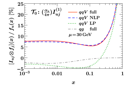
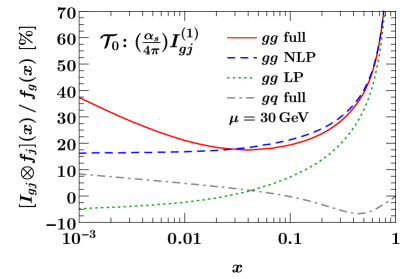
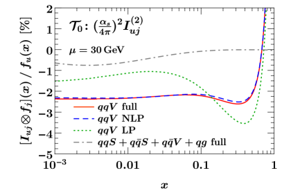
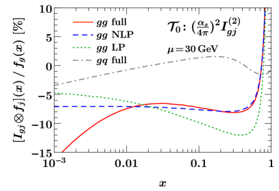
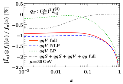
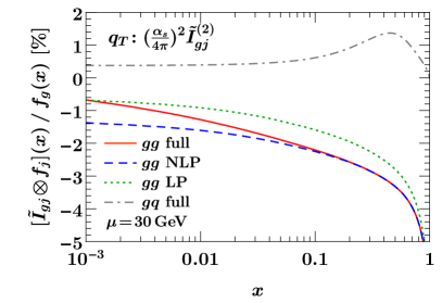
In figure -897, we compare the full 𝒯0subscript𝒯0\mathcal{T}_{0} beam function coefficient (solid) to its eikonal (LP dotted green) and next-to-eikonal (NLP dashed blue) expansions at NLO and NNLO for the u𝑢u quark and gluon channels. We always show the convolution (Iijfj)(x)/fi(x)tensor-productsubscript𝐼𝑖𝑗subscript𝑓𝑗𝑥subscript𝑓𝑖𝑥(I_{ij}\otimes f_{j})(x)/f_{i}(x) with the appropriate PDF fjsubscript𝑓𝑗f_{j} and normalize to the PDF fi(x)subscript𝑓𝑖𝑥f_{i}(x), corresponding to the LO result, where i=u𝑖𝑢i=u for the u𝑢u-quark case and i=g𝑖𝑔i=g for the gluon case. With this normalization, the shape gives an indication of the rapidity dependence of the beam function coefficient relative to the LO rapidity dependence induced by the shape of the PDFs. We also include the appropriate powers of αs/(4π)subscript𝛼𝑠4𝜋\alpha_{s}/(4\pi) at each order, so the overall normalization shows the percent impact relative to the LO result. For definiteness, we choose μ=30GeV𝜇30GeV\mu=30\,\,\mathrm{GeV} for the scale entering the PDFs and αssubscript𝛼𝑠\alpha_{s}.

The eikonal approximation reproduces the correct divergent behavior of the full flavor-diagonal contributions, denoted as qqV𝑞𝑞𝑉qqV and gg𝑔𝑔gg, toward large x𝑥x but is off away from large x𝑥x. On the other hand, including the next-to-eikonal terms yields an excellent approximation for all x𝑥x, particularly for the quark beam function. The rise at very small x𝑥x for the gluon, which is not reproduced at NLP, is due to the z0𝑧0z\to 0 divergent behavior in the gluon coefficient, which is not reproduced by its z1𝑧1z\to 1 expansion. If desired, it can be captured by including the leading z0𝑧0z\to 0 behavior of the coefficients, which for simplicity we refrain from doing here. For illustration, we also show the total contribution from all other corresponding nondiagonal channels (gray dot-dashed). In each case, they are numerically subdominant to the flavor-diagonal channel and also much flatter in x𝑥x, since they only start at NLP.

Refer to caption
Refer to caption
Refer to caption
Refer to caption
Figure -897: Comparison of the full beam function coefficients to their leading eikonal (LP) and next-to-eikonal (NLP) expansion at NLO (top) and NNLO (bottom). The u𝑢u-quark channel is shown on the left and the gluon channel on the right. In each case we also show the sum of all nondiagonal partonic channels for comparison.

The fact that the NLP result reproduces the full result very well, motivates us to construct an approximate ansatz for it, which we can then use at three loops to get a good estimate of the size of the unknown three-loop beam function coefficient beyond the eikonal limit.

We consider the following ansatz to approximate the coefficient,

Iij,approx(n)(z)superscriptsubscript𝐼𝑖𝑗approx𝑛𝑧\displaystyle I_{ij,\mathrm{approx}}^{(n)}(z) =IijLP(n)(z)+Iij,approxNLP(n)(z)+X2(1z)Iij,approxNLP(n)(z),absentsuperscriptsubscript𝐼𝑖𝑗LP𝑛𝑧superscriptsubscript𝐼𝑖𝑗approxNLP𝑛𝑧subscript𝑋21𝑧superscriptsubscript𝐼𝑖𝑗approxNLP𝑛𝑧\displaystyle=I_{ij}^{\mathrm{LP}(n)}(z)+I_{ij,\mathrm{approx}}^{\mathrm{NLP}(n)}(z)+X_{2}\,(1-z)I_{ij,\mathrm{approx}}^{\mathrm{NLP}(n)}(z)\,, (2.32)

where the NLP coefficient itself is approximated as

Iij,approxNLP(n)(z)superscriptsubscript𝐼𝑖𝑗approxNLP𝑛𝑧\displaystyle I_{ij,\mathrm{approx}}^{\mathrm{NLP}(n)}(z) =(1z)IijLP(n)(z)+X1(1z)dd(1z)[(1z)IijLP(n)(z)],absent1𝑧superscriptsubscript𝐼𝑖𝑗LP𝑛𝑧subscript𝑋11𝑧dd1𝑧delimited-[]1𝑧superscriptsubscript𝐼𝑖𝑗LP𝑛𝑧\displaystyle=-(1-z)I_{ij}^{\mathrm{LP}(n)}(z)+X_{1}\,(1-z)\frac{\mathrm{d}}{\mathrm{d}(1-z)}\Bigl{[}(1-z)I_{ij}^{\mathrm{LP}(n)}(z)\Bigr{]}\,, (2.33)

and X1subscript𝑋1X_{1} and X2subscript𝑋2X_{2} are free parameters that can be varied to estimate residual uncertainties. This ansatz is motivated by the known general logarithmic structure at NLP

IijNLP(n)(z)=k=02n1cn,kNLPlnk(1z).superscriptsubscript𝐼𝑖𝑗NLP𝑛𝑧superscriptsubscript𝑘02𝑛1superscriptsubscript𝑐𝑛𝑘NLPsuperscript𝑘1𝑧\displaystyle I_{ij}^{\mathrm{NLP}(n)}(z)=\sum_{k=0}^{2n-1}c_{n,k}^{\mathrm{NLP}}\ln^{k}(1-z)\,. (2.34)

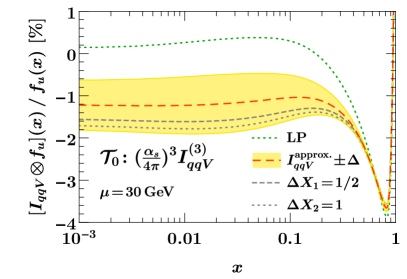
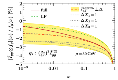
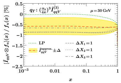
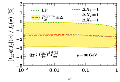
By multiplying the LP term by (1z)1𝑧(1-z) in eq. (2.33), we generate the appropriate logarithmic structure at NLP. The first term in eq. (2.33) reproduces the correct NLO and NNLO coefficients for the leading logarithm at NLP c1,1NLP=4Cisuperscriptsubscript𝑐11NLP4subscript𝐶𝑖c_{1,1}^{\mathrm{NLP}}=-4C_{i} and c2,3NLP=8Ci2superscriptsubscript𝑐23NLP8superscriptsubscript𝐶𝑖2c_{2,3}^{\mathrm{NLP}}=-8C_{i}^{2} for both quarks and gluons. Here, the additional double logarithm is determined by the same power of (Γ0i)nsuperscriptsuperscriptsubscriptΓ0𝑖𝑛(\Gamma_{0}^{i})^{n} as at LP, and this pattern can be expected to hold at higher orders. The second term in eq. (2.33) generates a next-to-leading logarithmic NLP series. We fix the central value for X1=1subscript𝑋11X_{1}=1 to reproduce the NLL constant term at NLO c1,0=4Cisubscript𝑐104subscript𝐶𝑖c_{1,0}=4C_{i}. Interestingly, we find that this choice also reproduces all NNLO coefficients c2,ksubscript𝑐2𝑘c_{2,k} very well, typically to within 10%, for both quarks and gluons and also independently of the choice of nfsubscript𝑛𝑓n_{f}. This provides a very nontrivial check and so we expect that eq. (2.33) provides a very good model of the true NLP structure also at higher orders. To estimate the uncertainties, we vary X1subscript𝑋1X_{1} by ±0.5plus-or-minus0.5\pm 0.5, which effectively varies the coefficients of the subleading terms. At NNLO, this variation covers the exact value for all coefficients. In addition, the last term in eq. (2.32) estimates the possible effect of terms beyond NLP. Here, we simply take the central value X2=0subscript𝑋20X_{2}=0 and vary it by ±1plus-or-minus1\pm 1.

Since Xisubscript𝑋𝑖X_{i} probe independent structures, we can consider them as uncorrelated. Hence, we add the impacts ΔisubscriptΔ𝑖\Delta_{i} on the final result of their variation in quadrature

Δ=Δ1Δ2=Δ12+Δ22.Δdirect-sumsubscriptΔ1subscriptΔ2superscriptsubscriptΔ12superscriptsubscriptΔ22\displaystyle\Delta=\Delta_{1}\oplus\Delta_{2}=\sqrt{\Delta_{1}^{2}+\Delta_{2}^{2}}\,. (2.35)
Refer to caption
Refer to caption
Refer to caption
Refer to caption
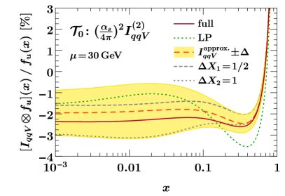
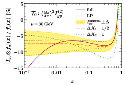
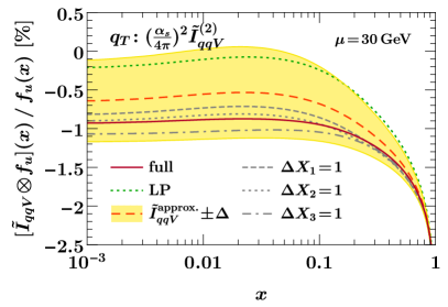
Figure -896: Approximate ansatzes for the NNLO (top) and N3LO (bottom) kernels, in the u𝑢u-quark (left) and gluon (right) channels.

In figure -896, we show the approximate kernel at NNLO (top) and N3LO (bottom) for the u𝑢u-quark (left) and gluon (right) channels. The dashed orange line shows the central result from our ansatz and the yellow band its estimated uncertainty. The gray lines show the impact of the individual variations of the Xisubscript𝑋𝑖X_{i} as indicated. In the top panel (NNLO), we also show the known full two-loop results (red solid). It shows that the ansatz including uncertainties approximates the true result very well, except for the gluon at very small x𝑥x where we do not expect it to hold.

At N3LO, we see that the approximate result gives rise to a sizable shift from the pure eikonal limit, which we believe to be genuine. Hence, we expect the full three-loop coefficients to have a nontrivial impact in the one to few percent range. The uncertainties at N3LO are reduced compared to NNLO as expected, but are still sizable, which adds motivation for the exact calculation of the full three-loop coefficients.

3 qTsubscript𝑞𝑇q_{T} factorization to three loops

3.1 Factorization theorem

The factorization of the qTsubscript𝑞𝑇{\vec{q}}_{T} distribution in the limit qT|qT|Qsubscript𝑞𝑇subscript𝑞𝑇much-less-than𝑄q_{T}\equiv\lvert{\vec{q}}_{T}\rvert\ll Q was first established by Collins, Soper, and Sterman (CSS) [119, 120, 48], and was later elaborated on in refs. [121, 122, 123, 124]. The factorization for qTsubscript𝑞𝑇q_{T} was also shown within the framework of SCET in refs. [125, 126, 127, 117]. Sometimes it is also referred to as transverse-momentum dependent (TMD) factorization. We write the factorized cross section as

dσdQ2dYd2qTd𝜎dsuperscript𝑄2d𝑌superscriptd2subscript𝑞𝑇\displaystyle\frac{\mathrm{d}\sigma}{\mathrm{d}Q^{2}\mathrm{d}Y\mathrm{d}^{2}{\vec{q}}_{T}} =d2bTeiqTbTdσ~sing(bT)dQ2dY[1+𝒪(qT2Q2)],absentsuperscriptd2subscript𝑏𝑇superscript𝑒isubscript𝑞𝑇subscript𝑏𝑇dsuperscript~𝜎singsubscript𝑏𝑇dsuperscript𝑄2d𝑌delimited-[]1𝒪superscriptsubscript𝑞𝑇2superscript𝑄2\displaystyle=\int\!\mathrm{d}^{2}{\vec{b}}_{T}\,e^{\mathrm{i}\,{\vec{q}}_{T}\cdot{\vec{b}}_{T}}\,\frac{\mathrm{d}\tilde{\sigma}^{\mathrm{sing}}(\vec{b}_{T})}{\mathrm{d}Q^{2}\mathrm{d}Y}\Bigl{[}1+\mathcal{O}\Bigl{(}\frac{q_{T}^{2}}{Q^{2}}\Bigr{)}\Bigr{]}\,,
dσ~sing(bT)dQ2dYdsuperscript~𝜎singsubscript𝑏𝑇dsuperscript𝑄2d𝑌\displaystyle\frac{\mathrm{d}\tilde{\sigma}^{\mathrm{sing}}(\vec{b}_{T})}{\mathrm{d}Q^{2}\mathrm{d}Y} =a,bHab(Q2,μ)B~a(xa,bT,μ,ν)B~b(xb,bT,μ,ν)S~i(bT,μ,ν).absentsubscript𝑎𝑏subscript𝐻𝑎𝑏superscript𝑄2𝜇subscript~𝐵𝑎subscript𝑥𝑎subscript𝑏𝑇𝜇𝜈subscript~𝐵𝑏subscript𝑥𝑏subscript𝑏𝑇𝜇𝜈subscript~𝑆𝑖subscript𝑏𝑇𝜇𝜈\displaystyle=\sum_{a,b}H_{ab}(Q^{2},\mu)\tilde{B}_{a}(x_{a},{\vec{b}}_{T},\mu,\nu)\,\tilde{B}_{b}(x_{b},{\vec{b}}_{T},\mu,\nu)\,\tilde{S}_{i}(b_{T},\mu,\nu)\,. (3.1)

It receives power corrections suppressed by qT2/Q2superscriptsubscript𝑞𝑇2superscript𝑄2q_{T}^{2}/Q^{2} as indicated. As is common, we consider the factorized singular cross section in Fourier-conjugate bTsubscript𝑏𝑇{\vec{b}}_{T} space, where convolutions in qTsubscript𝑞𝑇{\vec{q}}_{T} space turn into simple products. In particular, Fourier transforming the qTsubscript𝑞𝑇{\vec{q}}_{T}-dependent plus distributions n(qT,μ)subscript𝑛subscript𝑞𝑇𝜇\mathcal{L}_{n}({\vec{q}}_{T},\mu) turns them into powers of the canonical bTsubscript𝑏𝑇{\vec{b}}_{T}-space logarithms, which we denote as

Lb=lnbT2μ2b02,b0=2eγE.formulae-sequencesubscript𝐿𝑏superscriptsubscript𝑏𝑇2superscript𝜇2superscriptsubscript𝑏02subscript𝑏02superscript𝑒subscript𝛾𝐸L_{b}=\ln\frac{b_{T}^{2}\mu^{2}}{b_{0}^{2}}\,,\qquad b_{0}=2e^{-\gamma_{E}}\,. (3.2)

More details on their Fourier transformation are given in appendix A.2.

The qTsubscript𝑞𝑇q_{T} factorization is affected by rapidity divergences that must be regulated by a dedicated rapidity regulator. This gives rise to an additional rapidity scale, denoted as ν𝜈\nu in eq. (3.1). We use the exponential regulator of ref. [117], which up to two loops gives results equivalent to the η𝜂\eta regulator of refs. [128, 127].

The beam function appearing in eq. (3.1) is the inclusive transverse-momentum dependent (SCETII) beam function, which also appears in the qTsubscript𝑞𝑇q_{T} factorization of Z+j𝑍𝑗Z+j and γ+j𝛾𝑗\gamma+j [129, 130]. The qTsubscript𝑞𝑇q_{T}-dependent soft function in eq. (3.1) is the renormalized vacuum matrix element of two incoming soft Wilson lines. Note that for simplicity, we generically refer to them as qTsubscript𝑞𝑇q_{T} beam and soft functions, even though we mostly consider their bTsubscript𝑏𝑇b_{T}-dependent Fourier conjugates. The qTsubscript𝑞𝑇q_{T} beam and soft functions are known at two loops for several regulators [131, 132, 133, 134, 135, 136, 137, 138]. The soft function is known at three loops using the exponential regulator [82].

We also note that one can equivalently define ν𝜈\nu-independent TMDPDFs as

f~i(x,bT,μ,ζ)=B~i(x,bT,μ,ν)S~i(bT,μ,ν),ζ=ω2=(xEcm)2,formulae-sequencesubscript~𝑓𝑖𝑥subscript𝑏𝑇𝜇𝜁subscript~𝐵𝑖𝑥subscript𝑏𝑇𝜇𝜈subscript~𝑆𝑖subscript𝑏𝑇𝜇𝜈𝜁superscript𝜔2superscript𝑥subscript𝐸cm2\tilde{f}_{i}(x,{\vec{b}}_{T},\mu,\zeta)=\tilde{B}_{i}(x,{\vec{b}}_{T},\mu,\nu)\sqrt{\tilde{S}_{i}(b_{T},\mu,\nu)}\,,\qquad\zeta=\omega^{2}=(xE_{\mathrm{cm}})^{2}\,, (3.3)

as is done e.g. in refs. [48, 121, 122, 123, 124, 125, 126]. Here, the Collins-Soper scale [119, 120] ζ=ω2𝜁superscript𝜔2\zeta=\omega^{2} is given in terms of the lightcone momentum ω=xP𝜔𝑥superscript𝑃\omega=xP^{-} carried by the struck parton.

3.2 Rapidity anomalous dimension

The ν𝜈\nu dependence of the beam and soft functions is encoded in their rapidity RGEs [127],

νddνB~i(x,bT,μ,ν)𝜈dd𝜈subscript~𝐵𝑖𝑥subscript𝑏𝑇𝜇𝜈\displaystyle\nu\frac{\mathrm{d}}{\mathrm{d}\nu}\tilde{B}_{i}(x,{\vec{b}}_{T},\mu,\nu) =γ~ν,Bi(bT,μ)B~i(x,bT,μ,ν),absentsuperscriptsubscript~𝛾𝜈𝐵𝑖subscript𝑏𝑇𝜇subscript~𝐵𝑖𝑥subscript𝑏𝑇𝜇𝜈\displaystyle=\tilde{\gamma}_{\nu,B}^{i}(b_{T},\mu)\,\tilde{B}_{i}(x,{\vec{b}}_{T},\mu,\nu)\,,
νddνS~i(bT,μ,ν)𝜈dd𝜈subscript~𝑆𝑖subscript𝑏𝑇𝜇𝜈\displaystyle\nu\frac{\mathrm{d}}{\mathrm{d}\nu}\tilde{S}_{i}(b_{T},\mu,\nu) =γ~ν,Si(bT,μ)S~i(bT,μ,ν),absentsuperscriptsubscript~𝛾𝜈𝑆𝑖subscript𝑏𝑇𝜇subscript~𝑆𝑖subscript𝑏𝑇𝜇𝜈\displaystyle=\tilde{\gamma}_{\nu,S}^{i}(b_{T},\mu)\,\tilde{S}_{i}(b_{T},\mu,\nu)\,, (3.4)

where γ~ν,Bisuperscriptsubscript~𝛾𝜈𝐵𝑖\tilde{\gamma}_{\nu,B}^{i} and γ~ν,Sisuperscriptsubscript~𝛾𝜈𝑆𝑖\tilde{\gamma}_{\nu,S}^{i} are the beam and soft rapidity anomalous dimensions, which are closely related to the Collins-Soper kernel [119, 120]. Because the cross section in eq. (3.1) is independent of ν𝜈\nu, they are related by

γ~νi(bT,μ)γ~ν,Si(bT,μ)=2γ~ν,Bi(bT,μ),superscriptsubscript~𝛾𝜈𝑖subscript𝑏𝑇𝜇superscriptsubscript~𝛾𝜈𝑆𝑖subscript𝑏𝑇𝜇2superscriptsubscript~𝛾𝜈𝐵𝑖subscript𝑏𝑇𝜇\displaystyle\tilde{\gamma}_{\nu}^{i}(b_{T},\mu)\equiv\tilde{\gamma}_{\nu,S}^{i}(b_{T},\mu)=-2\tilde{\gamma}_{\nu,B}^{i}(b_{T},\mu)\,, (3.5)

and we will simply refer to γ~νi(bT,μ)superscriptsubscript~𝛾𝜈𝑖subscript𝑏𝑇𝜇\tilde{\gamma}_{\nu}^{i}(b_{T},\mu) as the rapidity anomalous dimension.

An important property of γ~νi(bT,μ)superscriptsubscript~𝛾𝜈𝑖subscript𝑏𝑇𝜇\tilde{\gamma}_{\nu}^{i}(b_{T},\mu) is that like the soft function it only depends on the color representation i={q,g}𝑖𝑞𝑔i=\{q,g\} but not on the specific massless quark flavor. While we only need its fixed-order expansion, we note that it becomes genuinely nonperturbative for bT1ΛQCDless-than-or-similar-tosuperscriptsubscript𝑏𝑇1subscriptΛQCDb_{T}^{-1}\lesssim\Lambda_{\rm QCD}, and recently a proposal was made to calculate it nonperturbatively using lattice QCD [139, 140].

The rapidity anomalous dimension itself satisfies an RGE in μ𝜇\mu,

μddμγ~νi(bT,μ)=4Γcuspi[αs(μ)],𝜇dd𝜇subscriptsuperscript~𝛾𝑖𝜈subscript𝑏𝑇𝜇4superscriptsubscriptΓcusp𝑖delimited-[]subscript𝛼𝑠𝜇\displaystyle\mu\frac{\mathrm{d}}{\mathrm{d}\mu}\tilde{\gamma}^{i}_{\nu}(b_{T},\mu)=-4\Gamma_{\mathrm{cusp}}^{i}[\alpha_{s}(\mu)]\,, (3.6)

which predicts its all-order structure in bTsubscript𝑏𝑇b_{T} and μ𝜇\mu. Similar to the 𝒯0subscript𝒯0\mathcal{T}_{0} soft function in section 2.2, it can be solved recursively order by order in αssubscript𝛼𝑠\alpha_{s}. Expanding both sides of eq. (3.6) to fixed order in αs(μ)subscript𝛼𝑠𝜇\alpha_{s}(\mu) and accounting for the running of αs(μ)subscript𝛼𝑠𝜇\alpha_{s}(\mu), the (n+1)𝑛1(n+1)-loop term is related to the lower-order terms by

γ~νi(n+1)(bT,μ)=2Γn+1iLb+m=0n2(m+1)βnmb0/bTμdμμγ~νi(m)(bT,μ)+γ~νn+1i,superscriptsubscript~𝛾𝜈𝑖𝑛1subscript𝑏𝑇𝜇2subscriptsuperscriptΓ𝑖𝑛1subscript𝐿𝑏superscriptsubscript𝑚0𝑛2𝑚1subscript𝛽𝑛𝑚superscriptsubscriptsubscript𝑏0subscript𝑏𝑇𝜇dsuperscript𝜇superscript𝜇superscriptsubscript~𝛾𝜈𝑖𝑚subscript𝑏𝑇superscript𝜇superscriptsubscript~𝛾𝜈𝑛1𝑖\tilde{\gamma}_{\nu}^{i\,(n+1)}(b_{T},\mu)=-2\Gamma^{i}_{n+1}L_{b}+\sum_{m=0}^{n}2(m+1)\,\beta_{n-m}\int_{b_{0}/b_{T}}^{\mu}\!\frac{\mathrm{d}\mu^{\prime}}{\mu^{\prime}}\,\tilde{\gamma}_{\nu}^{i\,(m)}(b_{T},\mu^{\prime})+\tilde{\gamma}_{\nu\,n+1}^{i}\,, (3.7)

where the nonlogarithmic boundary coefficients are defined as

γ~νni=γ~νi(n)(bT,μ=b0/bT).superscriptsubscript~𝛾𝜈𝑛𝑖superscriptsubscript~𝛾𝜈𝑖𝑛subscript𝑏𝑇𝜇subscript𝑏0subscript𝑏𝑇\tilde{\gamma}_{\nu\,n}^{i}=\tilde{\gamma}_{\nu}^{i\,(n)}(b_{T},\mu=b_{0}/b_{T})\,. (3.8)

The result up to three loops is

γ~νi(0)(bT,μ)superscriptsubscript~𝛾𝜈𝑖0subscript𝑏𝑇𝜇\displaystyle\tilde{\gamma}_{\nu}^{i\,(0)}(b_{T},\mu) =Lb 2Γ0i+γ~ν 0i,absentsubscript𝐿𝑏2superscriptsubscriptΓ0𝑖superscriptsubscript~𝛾𝜈 0𝑖\displaystyle=-L_{b}\,2\Gamma_{0}^{i}+\tilde{\gamma}_{\nu\,0}^{i}\,,
γ~νi(1)(bT,μ)superscriptsubscript~𝛾𝜈𝑖1subscript𝑏𝑇𝜇\displaystyle\tilde{\gamma}_{\nu}^{i\,(1)}(b_{T},\mu) =Lb2Γ0iβ0+Lb(β0γ~ν 0i2Γ1i)+γ~ν 1i,absentsuperscriptsubscript𝐿𝑏2superscriptsubscriptΓ0𝑖subscript𝛽0subscript𝐿𝑏subscript𝛽0superscriptsubscript~𝛾𝜈 0𝑖2superscriptsubscriptΓ1𝑖superscriptsubscript~𝛾𝜈1𝑖\displaystyle=-L_{b}^{2}\,\Gamma_{0}^{i}\beta_{0}+L_{b}\bigl{(}\beta_{0}\tilde{\gamma}_{\nu\,0}^{i}-2\Gamma_{1}^{i}\bigr{)}+\tilde{\gamma}_{\nu\,1}^{i}\,,
γ~νi(2)(bT,μ)superscriptsubscript~𝛾𝜈𝑖2subscript𝑏𝑇𝜇\displaystyle\tilde{\gamma}_{\nu}^{i\,(2)}(b_{T},\mu) =Lb323Γ0iβ02+Lb2(β02γ~ν 0i2Γ1iβ0Γ0iβ1)+Lb(2β0γ~ν 1i+β1γ~ν 0i2Γ2i)absentsuperscriptsubscript𝐿𝑏323superscriptsubscriptΓ0𝑖superscriptsubscript𝛽02superscriptsubscript𝐿𝑏2superscriptsubscript𝛽02superscriptsubscript~𝛾𝜈 0𝑖2superscriptsubscriptΓ1𝑖subscript𝛽0superscriptsubscriptΓ0𝑖subscript𝛽1subscript𝐿𝑏2subscript𝛽0superscriptsubscript~𝛾𝜈1𝑖subscript𝛽1superscriptsubscript~𝛾𝜈 0𝑖2superscriptsubscriptΓ2𝑖\displaystyle=-L_{b}^{3}\,\frac{2}{3}\Gamma_{0}^{i}\beta_{0}^{2}+L_{b}^{2}\bigl{(}\beta_{0}^{2}\tilde{\gamma}_{\nu\,0}^{i}-2\Gamma_{1}^{i}\beta_{0}-\Gamma_{0}^{i}\beta_{1}\bigr{)}+L_{b}\bigl{(}2\beta_{0}\tilde{\gamma}_{\nu\,1}^{i}+\beta_{1}\tilde{\gamma}_{\nu\,0}^{i}-2\Gamma_{2}^{i}\bigr{)}
+γ~ν 2i.superscriptsubscript~𝛾𝜈2𝑖\displaystyle\quad+\tilde{\gamma}_{\nu\,2}^{i}\,. (3.9)

The boundary coefficients γ~νnisuperscriptsubscript~𝛾𝜈𝑛𝑖\tilde{\gamma}_{\nu\,n}^{i} are known up to three loops [136, 82, 141] and are summarized in eq. (D.3).

3.3 Soft function

The soft function is explicitly known to three loops [82]. For completeness, we explicitly derive its fixed-order structure to illustrate the joint solution of its μ𝜇\mu and ν𝜈\nu RGEs,

μddμS~i(bT,μ,ν)𝜇dd𝜇subscript~𝑆𝑖subscript𝑏𝑇𝜇𝜈\displaystyle\mu\frac{\mathrm{d}}{\mathrm{d}\mu}\tilde{S}_{i}(b_{T},\mu,\nu) =γ~Si(μ,ν)S~i(bT,μ,ν),absentsuperscriptsubscript~𝛾𝑆𝑖𝜇𝜈subscript~𝑆𝑖subscript𝑏𝑇𝜇𝜈\displaystyle=\tilde{\gamma}_{S}^{i}(\mu,\nu)\,\tilde{S}_{i}(b_{T},\mu,\nu)\,,
νddνS~i(bT,μ,ν)𝜈dd𝜈subscript~𝑆𝑖subscript𝑏𝑇𝜇𝜈\displaystyle\nu\frac{\mathrm{d}}{\mathrm{d}\nu}\tilde{S}_{i}(b_{T},\mu,\nu) =γ~νi(bT,μ)S~i(bT,μ,ν).absentsuperscriptsubscript~𝛾𝜈𝑖subscript𝑏𝑇𝜇subscript~𝑆𝑖subscript𝑏𝑇𝜇𝜈\displaystyle=\tilde{\gamma}_{\nu}^{i}(b_{T},\mu)\,\tilde{S}_{i}(b_{T},\mu,\nu)\,. (3.10)

The perturbative structure of γνisuperscriptsubscript𝛾𝜈𝑖\gamma_{\nu}^{i} is discussed in section 3.2 above. The μ𝜇\mu anomalous dimension has the all-order structure

γ~Si(μ,ν)=4Γcuspi[αs(μ)]lnμν+γ~Si[αs(μ)],superscriptsubscript~𝛾𝑆𝑖𝜇𝜈4superscriptsubscriptΓcusp𝑖delimited-[]subscript𝛼𝑠𝜇𝜇𝜈superscriptsubscript~𝛾𝑆𝑖delimited-[]subscript𝛼𝑠𝜇\tilde{\gamma}_{S}^{i}(\mu,\nu)=4\Gamma_{\mathrm{cusp}}^{i}[\alpha_{s}(\mu)]\ln\frac{\mu}{\nu}+\tilde{\gamma}_{S}^{i}[\alpha_{s}(\mu)]\,, (3.11)

where Γcuspi(αs)superscriptsubscriptΓcusp𝑖subscript𝛼𝑠\Gamma_{\mathrm{cusp}}^{i}(\alpha_{s}) and γ~Si(αs)superscriptsubscript~𝛾𝑆𝑖subscript𝛼𝑠\tilde{\gamma}_{S}^{i}(\alpha_{s}) are the cusp and the soft noncusp anomalous dimensions. Expanding both sides of eq. (3.3) order by order in αssubscript𝛼𝑠\alpha_{s}, we obtain the coupled RGEs

μddμS~i(n+1)(bT,μ,ν)𝜇dd𝜇superscriptsubscript~𝑆𝑖𝑛1subscript𝑏𝑇𝜇𝜈\displaystyle\mu\frac{\mathrm{d}}{\mathrm{d}\mu}{\tilde{S}_{i}^{(n+1)}(b_{T},\mu,\nu)} =m=0n(4Γnmilnμν+2mβnm+γ~Snmi)S~i(m)(bT,μ,ν),absentsuperscriptsubscript𝑚0𝑛4subscriptsuperscriptΓ𝑖𝑛𝑚𝜇𝜈2𝑚subscript𝛽𝑛𝑚superscriptsubscript~𝛾𝑆𝑛𝑚𝑖superscriptsubscript~𝑆𝑖𝑚subscript𝑏𝑇𝜇𝜈\displaystyle=\sum_{m=0}^{n}\Bigl{(}4\Gamma^{i}_{n-m}\ln\frac{\mu}{\nu}+2m\beta_{n-m}+\tilde{\gamma}_{S\,n-m}^{i}\Bigr{)}\tilde{S}_{i}^{(m)}(b_{T},\mu,\nu)\,,
νddνS~i(n+1)(bT,μ,ν)𝜈dd𝜈superscriptsubscript~𝑆𝑖𝑛1subscript𝑏𝑇𝜇𝜈\displaystyle\nu\frac{\mathrm{d}}{\mathrm{d}\nu}{\tilde{S}_{i}^{(n+1)}(b_{T},\mu,\nu)} =m=0nγ~νi(nm)(bT,μ)S~i(m)(bT,μ,ν).absentsuperscriptsubscript𝑚0𝑛superscriptsubscript~𝛾𝜈𝑖𝑛𝑚subscript𝑏𝑇𝜇superscriptsubscript~𝑆𝑖𝑚subscript𝑏𝑇𝜇𝜈\displaystyle=\sum_{m=0}^{n}\tilde{\gamma}_{\nu}^{i\,(n-m)}(b_{T},\mu)\,\tilde{S}_{i}^{(m)}(b_{T},\mu,\nu)\,. (3.12)

These are easily integrated to give

S~i(n+1)(bT,μ,ν)superscriptsubscript~𝑆𝑖𝑛1subscript𝑏𝑇𝜇𝜈\displaystyle\tilde{S}_{i}^{(n+1)}(b_{T},\mu,\nu) =m=0n[b0/bTμdμμ(4Γnmilnμν+2mβnm+γ~Snmi)S~i(m)(bT,μ,ν)\displaystyle=\sum_{m=0}^{n}\biggl{[}\int_{b_{0}/b_{T}}^{\mu}\!\frac{\mathrm{d}\mu^{\prime}}{\mu^{\prime}}\,\Bigl{(}4\Gamma^{i}_{n-m}\ln\frac{\mu^{\prime}}{\nu}+2m\beta_{n-m}+\tilde{\gamma}_{S\,n-m}^{i}\Bigr{)}\tilde{S}_{i}^{(m)}(b_{T},\mu^{\prime},\nu)
+b0/bTνdννγ~νnmiS~i(m)(bT,b0/bT,ν)]+s~i(n+1),\displaystyle\quad+\int_{b_{0}/b_{T}}^{\nu}\!\frac{\mathrm{d}\nu^{\prime}}{\nu^{\prime}}\,\tilde{\gamma}_{\nu\,n-m}^{i}\,\tilde{S}_{i}^{(m)}(b_{T},b_{0}/b_{T},\nu^{\prime})\biggr{]}+\tilde{s}_{i}^{(n+1)}\,, (3.13)

where we first integrated the ν𝜈\nu RGE at fixed μ=b0/bT𝜇subscript𝑏0subscript𝑏𝑇\mu=b_{0}/b_{T} and then the μ𝜇\mu RGE at arbitrary ν𝜈\nu. In this way, the rapidity anomalous dimension reduces to its boundary coefficients γνnisuperscriptsubscript𝛾𝜈𝑛𝑖\gamma_{\nu\,n}^{i}. The soft boundary coefficients in eq. (3.3) are defined as

s~i(n)=S~i(n)(bT,μ=b0/bT,ν=b0/bT).\tilde{s}_{i}^{(n)}=\tilde{S}_{i}^{(n)}(b_{T},\mu=b_{0}/b_{T},\nu=b_{0}/b_{T})\,. (3.14)

Starting from the LO result, s~i(0)=1superscriptsubscript~𝑠𝑖01\tilde{s}_{i}^{(0)}=1, and expressing the results in terms of

Lb=lnbT2μ2b02,b0=2eγE,Lν=lnμν,formulae-sequencesubscript𝐿𝑏superscriptsubscript𝑏𝑇2superscript𝜇2superscriptsubscript𝑏02formulae-sequencesubscript𝑏02superscript𝑒subscript𝛾𝐸subscript𝐿𝜈𝜇𝜈L_{b}=\ln\frac{b_{T}^{2}\mu^{2}}{b_{0}^{2}}\,,\quad b_{0}=2e^{-\gamma_{E}}\,,\qquad L_{\nu}=\ln\frac{\mu}{\nu}\,, (3.15)

eq. (3.3) yields up to two loops

S~i(0)(bT,μ,ν)superscriptsubscript~𝑆𝑖0subscript𝑏𝑇𝜇𝜈\displaystyle\tilde{S}_{i}^{(0)}(b_{T},\mu,\nu) =1,absent1\displaystyle=1\,,
S~i(1)(bT,μ,ν)superscriptsubscript~𝑆𝑖1subscript𝑏𝑇𝜇𝜈\displaystyle\tilde{S}_{i}^{(1)}(b_{T},\mu,\nu) =Lb2Γ0i2+Lb(Lν 2Γ0i+γ~S 0i2+γ~ν 0i2)Lνγ~ν 0i+s~i(1),absentsuperscriptsubscript𝐿𝑏2superscriptsubscriptΓ0𝑖2subscript𝐿𝑏subscript𝐿𝜈2superscriptsubscriptΓ0𝑖superscriptsubscript~𝛾𝑆 0𝑖2superscriptsubscript~𝛾𝜈 0𝑖2subscript𝐿𝜈superscriptsubscript~𝛾𝜈 0𝑖superscriptsubscript~𝑠𝑖1\displaystyle=-L_{b}^{2}\,\frac{\Gamma_{0}^{i}}{2}+L_{b}\Bigl{(}L_{\nu}\,2\Gamma_{0}^{i}+\frac{\tilde{\gamma}_{S\,0}^{i}}{2}+\frac{\tilde{\gamma}_{\nu\,0}^{i}}{2}\Bigr{)}-L_{\nu}\tilde{\gamma}_{\nu\,0}^{i}+\tilde{s}_{i}^{(1)}\,,
S~i(2)(bT,μ,ν)superscriptsubscript~𝑆𝑖2subscript𝑏𝑇𝜇𝜈\displaystyle\tilde{S}_{i}^{(2)}(b_{T},\mu,\nu) =Lb4(Γ0i)28Lb3Γ0i(LνΓ0i+β03+γ~S 0i4+γ~ν 0i4)absentsuperscriptsubscript𝐿𝑏4superscriptsuperscriptsubscriptΓ0𝑖28superscriptsubscript𝐿𝑏3superscriptsubscriptΓ0𝑖subscript𝐿𝜈superscriptsubscriptΓ0𝑖subscript𝛽03superscriptsubscript~𝛾𝑆 0𝑖4superscriptsubscript~𝛾𝜈 0𝑖4\displaystyle=L_{b}^{4}\,\frac{(\Gamma_{0}^{i})^{2}}{8}-L_{b}^{3}\,\Gamma_{0}^{i}\Bigl{(}L_{\nu}\Gamma_{0}^{i}+\frac{\beta_{0}}{3}+\frac{\tilde{\gamma}_{S\,0}^{i}}{4}+\frac{\tilde{\gamma}_{\nu\,0}^{i}}{4}\Bigr{)}
+Lb2[Lν2 2(Γ0i)2+LνΓ0i(β0+γ~S 0i+32γ~ν 0i)\displaystyle\quad+L_{b}^{2}\biggl{[}L_{\nu}^{2}\,2(\Gamma_{0}^{i})^{2}+L_{\nu}\Gamma_{0}^{i}\Bigl{(}\beta_{0}+\tilde{\gamma}_{S\,0}^{i}+\frac{3}{2}\tilde{\gamma}_{\nu\,0}^{i}\Bigr{)}
+β0(γ~S 0i4+γ~ν 0i2)+18(γ~S 0i+γ~ν 0i)2Γ1i2Γ0i2s~i(1)]\displaystyle\quad\hskip 25.83325pt+\beta_{0}\Bigl{(}\frac{\tilde{\gamma}_{S\,0}^{i}}{4}+\frac{\tilde{\gamma}_{\nu\,0}^{i}}{2}\Bigr{)}+\frac{1}{8}(\tilde{\gamma}_{S\,0}^{i}+\tilde{\gamma}_{\nu\,0}^{i})^{2}-\frac{\Gamma_{1}^{i}}{2}-\frac{\Gamma_{0}^{i}}{2}\,\tilde{s}_{i}^{(1)}\biggr{]}
+Lb{Lν2 2Γ0iγ~ν 0i+Lν[(β0+γ~S 0i2+γ~ν 0i2)γ~ν 0i+2Γ1i+2Γ0is~i(1)]\displaystyle\quad+L_{b}\biggl{\{}-L_{\nu}^{2}\,2\Gamma_{0}^{i}\tilde{\gamma}_{\nu\,0}^{i}+L_{\nu}\Bigl{[}-\Bigl{(}\beta_{0}+\frac{\tilde{\gamma}_{S\,0}^{i}}{2}+\frac{\tilde{\gamma}_{\nu\,0}^{i}}{2}\Bigr{)}\tilde{\gamma}_{\nu\,0}^{i}+2\Gamma_{1}^{i}+2\Gamma_{0}^{i}\,\tilde{s}_{i}^{(1)}\Bigr{]}
+γ~S 1i2+γ~ν 1i2+(β0+γ~S 0i2+γ~ν 0i2)s~i(1)}\displaystyle\quad\hskip 25.83325pt+\frac{\tilde{\gamma}_{S\,1}^{i}}{2}+\frac{\tilde{\gamma}_{\nu\,1}^{i}}{2}+\Bigl{(}\beta_{0}+\frac{\tilde{\gamma}_{S\,0}^{i}}{2}+\frac{\tilde{\gamma}_{\nu\,0}^{i}}{2}\Bigr{)}\tilde{s}_{i}^{(1)}\biggr{\}}
+Lν2(γ~ν 0i)22Lν(γ~ν 1i+γ~ν 0is~i(1))+s~i(2).superscriptsubscript𝐿𝜈2superscriptsuperscriptsubscript~𝛾𝜈 0𝑖22subscript𝐿𝜈superscriptsubscript~𝛾𝜈1𝑖superscriptsubscript~𝛾𝜈 0𝑖superscriptsubscript~𝑠𝑖1superscriptsubscript~𝑠𝑖2\displaystyle\quad+L_{\nu}^{2}\,\frac{(\tilde{\gamma}_{\nu\,0}^{i})^{2}}{2}-L_{\nu}\bigl{(}\tilde{\gamma}_{\nu\,1}^{i}+\tilde{\gamma}_{\nu\,0}^{i}\,\tilde{s}_{i}^{(1)}\bigr{)}+\tilde{s}_{i}^{(2)}\,. (3.16)

At three loops, we write the result as

S~i(3)(bT,μ,ν)==06S~i,(3)(Lν)Lb,superscriptsubscript~𝑆𝑖3subscript𝑏𝑇𝜇𝜈superscriptsubscript06superscriptsubscript~𝑆𝑖3subscript𝐿𝜈superscriptsubscript𝐿𝑏\tilde{S}_{i}^{(3)}(b_{T},\mu,\nu)=\sum_{\ell=0}^{6}\tilde{S}_{i,\ell}^{(3)}(L_{\nu})\,L_{b}^{\ell}\,, (3.17)

where the S~i,k(3)superscriptsubscript~𝑆𝑖𝑘3\tilde{S}_{i,k}^{(3)} coefficients themselves are polynomials in Lνsubscript𝐿𝜈L_{\nu}. Inserting γ~S 0i=γ~ν 0i=0superscriptsubscript~𝛾𝑆 0𝑖superscriptsubscript~𝛾𝜈 0𝑖0\tilde{\gamma}_{S\,0}^{i}=\tilde{\gamma}_{\nu\,0}^{i}=0 for brevity, they are given by

S~i,6(3)(Lν)superscriptsubscript~𝑆𝑖63subscript𝐿𝜈\displaystyle\tilde{S}_{i,6}^{(3)}(L_{\nu}) =(Γ0i)348,absentsuperscriptsubscriptsuperscriptΓ𝑖0348\displaystyle=-\frac{(\Gamma^{i}_{0})^{3}}{48}\,,
S~i,5(3)(Lν)superscriptsubscript~𝑆𝑖53subscript𝐿𝜈\displaystyle\tilde{S}_{i,5}^{(3)}(L_{\nu}) =Lν(Γ0i)34+(Γ0i)26β0,absentsubscript𝐿𝜈superscriptsubscriptsuperscriptΓ𝑖034superscriptsubscriptsuperscriptΓ𝑖026subscript𝛽0\displaystyle=L_{\nu}\,\frac{(\Gamma^{i}_{0})^{3}}{4}+\frac{(\Gamma^{i}_{0})^{2}}{6}\beta_{0}\,,
S~i,4(3)(Lν)superscriptsubscript~𝑆𝑖43subscript𝐿𝜈\displaystyle\tilde{S}_{i,4}^{(3)}(L_{\nu}) =Lν2(Γ0i)3Lν76(Γ0i)2β0+Γ0i4(β02+Γ1i+Γ0i2s~i(1)),absentsuperscriptsubscript𝐿𝜈2superscriptsubscriptsuperscriptΓ𝑖03subscript𝐿𝜈76superscriptsubscriptsuperscriptΓ𝑖02subscript𝛽0superscriptsubscriptΓ0𝑖4superscriptsubscript𝛽02subscriptsuperscriptΓ𝑖1subscriptsuperscriptΓ𝑖02superscriptsubscript~𝑠𝑖1\displaystyle=-L_{\nu}^{2}\,(\Gamma^{i}_{0})^{3}-L_{\nu}\,\frac{7}{6}(\Gamma^{i}_{0})^{2}\beta_{0}+\frac{\Gamma_{0}^{i}}{4}\Bigl{(}-\beta_{0}^{2}+\Gamma^{i}_{1}+\frac{\Gamma^{i}_{0}}{2}\,\tilde{s}_{i}^{(1)}\Bigr{)}\,,
S~i,3(3)(Lν)superscriptsubscript~𝑆𝑖33subscript𝐿𝜈\displaystyle\tilde{S}_{i,3}^{(3)}(L_{\nu}) =Lν343(Γ0i)3+Lν2 2(Γ0i)2β0+LνΓ0i(23β022Γ1iΓ0is~i(1))absentsuperscriptsubscript𝐿𝜈343superscriptsubscriptsuperscriptΓ𝑖03superscriptsubscript𝐿𝜈22superscriptsubscriptsuperscriptΓ𝑖02subscript𝛽0subscript𝐿𝜈superscriptsubscriptΓ0𝑖23superscriptsubscript𝛽022subscriptsuperscriptΓ𝑖1subscriptsuperscriptΓ𝑖0superscriptsubscript~𝑠𝑖1\displaystyle=L_{\nu}^{3}\,\frac{4}{3}(\Gamma^{i}_{0})^{3}+L_{\nu}^{2}\,2(\Gamma^{i}_{0})^{2}\beta_{0}+L_{\nu}\Gamma_{0}^{i}\Bigl{(}\frac{2}{3}\beta_{0}^{2}-2\Gamma^{i}_{1}-\Gamma^{i}_{0}\,\tilde{s}_{i}^{(1)}\Bigr{)}
23Γ1iβ0Γ0i(β13+γ~S 1i4+γ~ν 1i4+56β0s~i(1)),23subscriptsuperscriptΓ𝑖1subscript𝛽0superscriptsubscriptΓ0𝑖subscript𝛽13superscriptsubscript~𝛾𝑆1𝑖4superscriptsubscript~𝛾𝜈1𝑖456subscript𝛽0superscriptsubscript~𝑠𝑖1\displaystyle\quad-\frac{2}{3}\Gamma^{i}_{1}\beta_{0}-\Gamma_{0}^{i}\Bigl{(}\frac{\beta_{1}}{3}+\frac{\tilde{\gamma}_{S\,1}^{i}}{4}+\frac{\tilde{\gamma}_{\nu\,1}^{i}}{4}+\frac{5}{6}\beta_{0}\,\tilde{s}_{i}^{(1)}\Bigr{)}\,,
S~i,2(3)(Lν)superscriptsubscript~𝑆𝑖23subscript𝐿𝜈\displaystyle\tilde{S}_{i,2}^{(3)}(L_{\nu}) =Lν2Γ0i(4Γ1i+2Γ0is~i(1))+Lν[2Γ1iβ0+Γ0i(β1+γ~S 1i+32γ~ν 1i+3β0s~i(1))]absentsuperscriptsubscript𝐿𝜈2subscriptsuperscriptΓ𝑖04subscriptsuperscriptΓ𝑖12subscriptsuperscriptΓ𝑖0superscriptsubscript~𝑠𝑖1subscript𝐿𝜈delimited-[]2subscriptsuperscriptΓ𝑖1subscript𝛽0subscriptsuperscriptΓ𝑖0subscript𝛽1superscriptsubscript~𝛾𝑆1𝑖32superscriptsubscript~𝛾𝜈1𝑖3subscript𝛽0superscriptsubscript~𝑠𝑖1\displaystyle=L_{\nu}^{2}\,\Gamma^{i}_{0}\bigl{(}4\Gamma^{i}_{1}+2\Gamma^{i}_{0}\,\tilde{s}_{i}^{(1)}\bigr{)}+L_{\nu}\Bigl{[}2\Gamma^{i}_{1}\beta_{0}+\Gamma^{i}_{0}\Bigl{(}\beta_{1}+\tilde{\gamma}_{S\,1}^{i}+\frac{3}{2}\tilde{\gamma}_{\nu\,1}^{i}+3\beta_{0}\,\tilde{s}_{i}^{(1)}\Bigr{)}\Bigr{]}
+β0(γ~S 1i2+γ~ν 1i)Γ2i2+(β02Γ1i2)s~i(1)Γ0i2s~i(2),subscript𝛽0superscriptsubscript~𝛾𝑆1𝑖2superscriptsubscript~𝛾𝜈1𝑖subscriptsuperscriptΓ𝑖22superscriptsubscript𝛽02subscriptsuperscriptΓ𝑖12superscriptsubscript~𝑠𝑖1subscriptsuperscriptΓ𝑖02superscriptsubscript~𝑠𝑖2\displaystyle\quad+\beta_{0}\Bigl{(}\frac{\tilde{\gamma}_{S\,1}^{i}}{2}+\tilde{\gamma}_{\nu\,1}^{i}\Bigr{)}-\frac{\Gamma^{i}_{2}}{2}+\Bigl{(}\beta_{0}^{2}-\frac{\Gamma^{i}_{1}}{2}\Bigr{)}\tilde{s}_{i}^{(1)}-\frac{\Gamma^{i}_{0}}{2}\,\tilde{s}_{i}^{(2)}\,,
S~i,1(3)(Lν)superscriptsubscript~𝑆𝑖13subscript𝐿𝜈\displaystyle\tilde{S}_{i,1}^{(3)}(L_{\nu}) =Lν2 2Γ0iγ~ν 1i+Lν 2(β0γ~ν 1i+Γ2i+Γ1is~i(1)+Γ0is~i(2))absentsuperscriptsubscript𝐿𝜈22subscriptsuperscriptΓ𝑖0superscriptsubscript~𝛾𝜈1𝑖subscript𝐿𝜈2subscript𝛽0superscriptsubscript~𝛾𝜈1𝑖subscriptsuperscriptΓ𝑖2subscriptsuperscriptΓ𝑖1superscriptsubscript~𝑠𝑖1subscriptsuperscriptΓ𝑖0superscriptsubscript~𝑠𝑖2\displaystyle=-L_{\nu}^{2}\,2\Gamma^{i}_{0}\tilde{\gamma}_{\nu\,1}^{i}+L_{\nu}\,2\bigl{(}-\beta_{0}\tilde{\gamma}_{\nu\,1}^{i}+\Gamma^{i}_{2}+\Gamma^{i}_{1}\,\tilde{s}_{i}^{(1)}+\Gamma^{i}_{0}\,\tilde{s}_{i}^{(2)}\bigr{)}
+γ~S 2i2+γ~ν 2i2+(β1+γ~S 1i2+γ~ν 1i2)s~i(1)+2β0s~i(2),superscriptsubscript~𝛾𝑆2𝑖2superscriptsubscript~𝛾𝜈2𝑖2subscript𝛽1superscriptsubscript~𝛾𝑆1𝑖2superscriptsubscript~𝛾𝜈1𝑖2superscriptsubscript~𝑠𝑖12subscript𝛽0superscriptsubscript~𝑠𝑖2\displaystyle\quad+\frac{\tilde{\gamma}_{S\,2}^{i}}{2}+\frac{\tilde{\gamma}_{\nu\,2}^{i}}{2}+\Bigl{(}\beta_{1}+\frac{\tilde{\gamma}_{S\,1}^{i}}{2}+\frac{\tilde{\gamma}_{\nu\,1}^{i}}{2}\Bigr{)}\tilde{s}_{i}^{(1)}+2\beta_{0}\,\tilde{s}_{i}^{(2)}\,,
S~i,0(3)(Lν)superscriptsubscript~𝑆𝑖03subscript𝐿𝜈\displaystyle\tilde{S}_{i,0}^{(3)}(L_{\nu}) =Lν(γ~ν 2i+γ~ν 1is~i(1))+s~i(3).absentsubscript𝐿𝜈superscriptsubscript~𝛾𝜈2𝑖superscriptsubscript~𝛾𝜈1𝑖superscriptsubscript~𝑠𝑖1superscriptsubscript~𝑠𝑖3\displaystyle=-L_{\nu}\bigl{(}\tilde{\gamma}_{\nu\,2}^{i}+\tilde{\gamma}_{\nu\,1}^{i}\,\tilde{s}_{i}^{(1)}\bigr{)}+\tilde{s}_{i}^{(3)}\,. (3.18)

Eqs. (3.3) and (3.3) agree with refs. [136, 82]. The required anomalous dimension and boundary coefficients up to three loops are given in appendix D.3.

Numerical impact

The soft function S~i(bT,μ,ν)subscript~𝑆𝑖subscript𝑏𝑇𝜇𝜈\tilde{S}_{i}(b_{T},\mu,\nu) has an explicit dependence on the scales μ𝜇\mu and ν𝜈\nu that cancels against that of the hard and beam functions in eq. (3.1). Therefore, varying μ𝜇\mu and ν𝜈\nu is not very meaningful for illustrating the numerical impact of the scale-dependent three-loop terms. Instead, we consider the resummed soft function,

S~i(bT,μ,ν)subscript~𝑆𝑖subscript𝑏𝑇𝜇𝜈\displaystyle\tilde{S}_{i}(b_{T},\mu,\nu) =S~i(bT,μS,νS)U~Si(bT,μS,μ,νS,ν),absentsubscript~𝑆𝑖subscript𝑏𝑇subscript𝜇𝑆subscript𝜈𝑆superscriptsubscript~𝑈𝑆𝑖subscript𝑏𝑇subscript𝜇𝑆𝜇subscript𝜈𝑆𝜈\displaystyle=\tilde{S}_{i}(b_{T},\mu_{S},\nu_{S})\,\tilde{U}_{S}^{i}(b_{T},\mu_{S},\mu,\nu_{S},\nu)\,,
U~Si(bT,μS,μ,νS,ν)superscriptsubscript~𝑈𝑆𝑖subscript𝑏𝑇subscript𝜇𝑆𝜇subscript𝜈𝑆𝜈\displaystyle\tilde{U}_{S}^{i}(b_{T},\mu_{S},\mu,\nu_{S},\nu) =exp[lnννSγ~νi(bT,μS)]exp[μSμdμμγ~Si(μ,ν)],absent𝜈subscript𝜈𝑆superscriptsubscript~𝛾𝜈𝑖subscript𝑏𝑇subscript𝜇𝑆superscriptsubscriptsubscript𝜇𝑆𝜇dsuperscript𝜇superscript𝜇superscriptsubscript~𝛾𝑆𝑖superscript𝜇𝜈\displaystyle=\exp\biggl{[}\ln\frac{\nu}{\nu_{S}}\,\tilde{\gamma}_{\nu}^{i}(b_{T},\mu_{S})\biggr{]}\exp\biggl{[}\int_{\mu_{S}}^{\mu}\!\frac{\mathrm{d}\mu^{\prime}}{\mu^{\prime}}\,\tilde{\gamma}_{S}^{i}(\mu^{\prime},\nu)\biggr{]}\,, (3.19)

where we have chosen to first evolve in ν𝜈\nu and then in μ𝜇\mu.

To probe the full set of terms in the fixed-order expansion of S~i(bT,μS,νS)subscript~𝑆𝑖subscript𝑏𝑇subscript𝜇𝑆subscript𝜈𝑆\tilde{S}_{i}(b_{T},\mu_{S},\nu_{S}), we consider simultaneous variations of (μS,νS)subscript𝜇𝑆subscript𝜈𝑆(\mu_{S},\nu_{S}) around the canonical central scales μS=νS=μ=ν=b0/bTsubscript𝜇𝑆subscript𝜈𝑆𝜇𝜈subscript𝑏0subscript𝑏𝑇\mu_{S}=\nu_{S}=\mu=\nu=b_{0}/b_{T}. In figure -895 we show the residual scale dependence of the resummed soft function at the representative value b0/bT=20GeVsubscript𝑏0subscript𝑏𝑇20GeVb_{0}/b_{T}=20\,\mathrm{GeV} at NLL (dotted green), NNLL (dashed blue), and N3LL (solid orange), normalized to the NNLL result at the central scale. The three-loop finite term is included in figure -895, so the NNLL and N3LL results do not coincide at the central scales. We use four-loop running of αssubscript𝛼𝑠\alpha_{s} throughout, which formally amounts to a higher-order effect at (N)NLL. As expected, the scale dependence reduces from NLL to NNLL, where it is already quite small. At N3LL, it further stabilizes over a wider range of scales. As in section 2.2, we stress that the residual scale dependence in the resummed soft function by itself is not necessarily a good indicator of the perturbative uncertainty, but gives an indication of the typical reduction of perturbative uncertainties one might expect at each order.
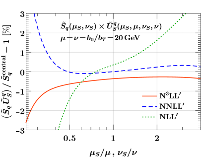
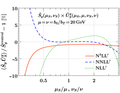
Refer to caption
Refer to caption
Figure -895: Residual scale dependence of the resummed qTsubscript𝑞𝑇q_{T} soft function in Fourier space for i=q𝑖𝑞i=q (left) and i=g𝑖𝑔i=g (right). Shown are the relative deviations from the NNLL result S~icentralsuperscriptsubscript~𝑆𝑖central\tilde{S}_{i}^{\mathrm{central}} at the central scales (μS,νS)=(μ,ν)=(b0/bT,b0/bT)subscript𝜇𝑆subscript𝜈𝑆𝜇𝜈subscript𝑏0subscript𝑏𝑇subscript𝑏0subscript𝑏𝑇(\mu_{S},\nu_{S})=(\mu,\nu)=(b_{0}/b_{T},b_{0}/b_{T}).

3.4 Beam function

The beam function obeys the coupled RGEs

μddμB~i(x,bT,μ,ν)𝜇dd𝜇subscript~𝐵𝑖𝑥subscript𝑏𝑇𝜇𝜈\displaystyle\mu\frac{\mathrm{d}}{\mathrm{d}\mu}{\tilde{B}_{i}(x,{\vec{b}}_{T},\mu,\nu)} =γ~Bi(μ,ν/ω)B~i(x,bT,μ,ν),absentsuperscriptsubscript~𝛾𝐵𝑖𝜇𝜈𝜔subscript~𝐵𝑖𝑥subscript𝑏𝑇𝜇𝜈\displaystyle=\tilde{\gamma}_{B}^{i}(\mu,\nu/\omega)\,\tilde{B}_{i}(x,{\vec{b}}_{T},\mu,\nu)\,,
νddνB~i(x,bT,μ,ν)𝜈dd𝜈subscript~𝐵𝑖𝑥subscript𝑏𝑇𝜇𝜈\displaystyle\nu\frac{\mathrm{d}}{\mathrm{d}\nu}{\tilde{B}_{i}(x,{\vec{b}}_{T},\mu,\nu)} =12γ~νi(bT,μ)B~i(x,bT,μ,ν),absent12superscriptsubscript~𝛾𝜈𝑖subscript𝑏𝑇𝜇subscript~𝐵𝑖𝑥subscript𝑏𝑇𝜇𝜈\displaystyle=-\frac{1}{2}\tilde{\gamma}_{\nu}^{i}(b_{T},\mu)\,\tilde{B}_{i}(x,{\vec{b}}_{T},\mu,\nu)\,, (3.20)

where the ν𝜈\nu anomalous dimension was discussed in section 3.2, and the μ𝜇\mu anomalous dimension has the all-order form

γ~Bi(μ,ν/ω)=2Γcuspi[αs(μ)]lnνω+γ~Bi[αs(μ)],superscriptsubscript~𝛾𝐵𝑖𝜇𝜈𝜔2superscriptsubscriptΓcusp𝑖delimited-[]subscript𝛼𝑠𝜇𝜈𝜔superscriptsubscript~𝛾𝐵𝑖delimited-[]subscript𝛼𝑠𝜇\tilde{\gamma}_{B}^{i}(\mu,\nu/\omega)=2\Gamma_{\mathrm{cusp}}^{i}[\alpha_{s}(\mu)]\ln\frac{\nu}{\omega}+\tilde{\gamma}_{B}^{i}[\alpha_{s}(\mu)]\,, (3.21)

where Γcuspi(αs)superscriptsubscriptΓcusp𝑖subscript𝛼𝑠\Gamma_{\mathrm{cusp}}^{i}(\alpha_{s}) and γ~Bi(αs)superscriptsubscript~𝛾𝐵𝑖subscript𝛼𝑠\tilde{\gamma}_{B}^{i}(\alpha_{s}) are the cusp and the beam noncusp anomalous dimensions.

For perturbative b0/bTΛQCDmuch-greater-thansubscript𝑏0subscript𝑏𝑇subscriptΛQCDb_{0}/b_{T}\gg\Lambda_{\mathrm{QCD}}, the TMD beam function satisfies an OPE in terms of standard PDFs [48],

B~q(x,bT,μ,ν)subscript~𝐵𝑞𝑥subscript𝑏𝑇𝜇𝜈\displaystyle\tilde{B}_{q}(x,b_{T},\mu,\nu) =jdzz~qj(z,bT,μ,ν/ω)fj(xz,μ)[1+𝒪(bTΛQCD)],absentsubscript𝑗d𝑧𝑧subscript~𝑞𝑗𝑧subscript𝑏𝑇𝜇𝜈𝜔subscript𝑓𝑗𝑥𝑧𝜇delimited-[]1𝒪subscript𝑏𝑇subscriptΛQCD\displaystyle=\sum_{j}\int\!\frac{\mathrm{d}z}{z}\,\tilde{\mathcal{I}}_{qj}(z,b_{T},\mu,\nu/\omega)f_{j}\Bigl{(}\frac{x}{z},\mu\Bigr{)}\bigl{[}1+\mathcal{O}(b_{T}\Lambda_{\mathrm{QCD}})\bigr{]}\,,
B~gρλ(x,bT,μ,ν)subscriptsuperscript~𝐵𝜌𝜆𝑔𝑥subscript𝑏𝑇𝜇𝜈\displaystyle\tilde{B}^{\rho\lambda}_{g}(x,{\vec{b}}_{T},\mu,\nu) =jdzz[gρλ2~gj(z,bT,μ,ν/ω)+(gρλ2bρbλb2)𝒥~gj(z,bT,μ,ν/ω)]absentsubscript𝑗d𝑧𝑧delimited-[]superscriptsubscript𝑔perpendicular-to𝜌𝜆2subscript~𝑔𝑗𝑧subscript𝑏𝑇𝜇𝜈𝜔superscriptsubscript𝑔perpendicular-to𝜌𝜆2superscriptsubscript𝑏perpendicular-to𝜌superscriptsubscript𝑏perpendicular-to𝜆superscriptsubscript𝑏perpendicular-to2subscript~𝒥𝑔𝑗𝑧subscript𝑏𝑇𝜇𝜈𝜔\displaystyle=\sum_{j}\int\!\frac{\mathrm{d}z}{z}\biggl{[}\frac{g_{\perp}^{\rho\lambda}}{2}\,\tilde{\mathcal{I}}_{gj}(z,b_{T},\mu,\nu/\omega)+\biggl{(}\frac{g_{\perp}^{\rho\lambda}}{2}-\frac{b_{\perp}^{\rho}b_{\perp}^{\lambda}}{b_{\perp}^{2}}\biggr{)}\tilde{\mathcal{J}}_{gj}(z,b_{T},\mu,\nu/\omega)\biggr{]}
×fj(xz,μ)[1+𝒪(bTΛQCD)].absentsubscript𝑓𝑗𝑥𝑧𝜇delimited-[]1𝒪subscript𝑏𝑇subscriptΛQCD\displaystyle\quad\hskip 43.05542pt\times f_{j}\Bigl{(}\frac{x}{z},\mu\Bigr{)}\bigl{[}1+\mathcal{O}(b_{T}\Lambda_{\mathrm{QCD}})\bigr{]}\,. (3.22)

For the gluon beam function, we have made its dependence on the gluon helicity explicit, and decomposed it into two orthogonal structures, namely the polarization-independent piece ~gjsubscript~𝑔𝑗\tilde{\mathcal{I}}_{gj} and the polarization-dependent piece 𝒥~gjsubscript~𝒥𝑔𝑗\tilde{\mathcal{J}}_{gj}, where gρλ=gρλ(nρn¯λ+n¯ρnλ)/2superscriptsubscript𝑔perpendicular-to𝜌𝜆superscript𝑔𝜌𝜆superscript𝑛𝜌superscript¯𝑛𝜆superscript¯𝑛𝜌superscript𝑛𝜆2g_{\perp}^{\rho\lambda}=g^{\rho\lambda}-(n^{\rho}{\bar{n}}^{\lambda}+{\bar{n}}^{\rho}n^{\lambda})/2 is the transverse metric and bρsuperscriptsubscript𝑏perpendicular-to𝜌b_{\perp}^{\rho} is the transverse four vector with b2=bT2superscriptsubscript𝑏perpendicular-to2superscriptsubscript𝑏𝑇2b_{\perp}^{2}=-{\vec{b}}_{T}^{2}. Due to the multiplicative structure of eq. (3.4), both ~gjsubscript~𝑔𝑗\tilde{\mathcal{I}}_{gj} and 𝒥~gjsubscript~𝒥𝑔𝑗\tilde{\mathcal{J}}_{gj} obey the same RGE, and in the following we will only consider the RGEs for ~ijsubscript~𝑖𝑗\tilde{\mathcal{I}}_{ij}.

The ~ijsubscript~𝑖𝑗\tilde{\mathcal{I}}_{ij} are perturbatively calculable matching coefficients, whose RGEs follow from eq. (3.4) by taking the evolution of the PDFs into account,

μddμ~ij(z,bT,μ,ν/ω)𝜇dd𝜇subscript~𝑖𝑗𝑧subscript𝑏𝑇𝜇𝜈𝜔\displaystyle\mu\frac{\mathrm{d}}{\mathrm{d}\mu}{\tilde{\mathcal{I}}_{ij}(z,b_{T},\mu,\nu/\omega)} =kdzz~ik(zz,bT,μ,ν/ω)[γ~Bi(μ,ν/ω)𝟏kj(z)2Pkj(z,μ)],absentsubscript𝑘dsuperscript𝑧superscript𝑧subscript~𝑖𝑘𝑧superscript𝑧subscript𝑏𝑇𝜇𝜈𝜔delimited-[]superscriptsubscript~𝛾𝐵𝑖𝜇𝜈𝜔subscript1𝑘𝑗superscript𝑧2subscript𝑃𝑘𝑗superscript𝑧𝜇\displaystyle=\sum_{k}\int\!\frac{\mathrm{d}z^{\prime}}{z^{\prime}}\,\tilde{\mathcal{I}}_{ik}\Bigl{(}\frac{z}{z^{\prime}},b_{T},\mu,\nu/\omega\Bigr{)}\bigl{[}\tilde{\gamma}_{B}^{i}(\mu,\nu/\omega)\mathbf{1}_{kj}(z^{\prime})-2P_{kj}(z^{\prime},\mu)\bigr{]}\,,
νddν~ij(z,bT,μ,ν/ω)𝜈dd𝜈subscript~𝑖𝑗𝑧subscript𝑏𝑇𝜇𝜈𝜔\displaystyle\nu\frac{\mathrm{d}}{\mathrm{d}\nu}{\tilde{\mathcal{I}}_{ij}(z,b_{T},\mu,\nu/\omega)} =12γ~νi(bT,μ)~ij(z,bT,μ,ν/ω).absent12superscriptsubscript~𝛾𝜈𝑖subscript𝑏𝑇𝜇subscript~𝑖𝑗𝑧subscript𝑏𝑇𝜇𝜈𝜔\displaystyle=-\frac{1}{2}\tilde{\gamma}_{\nu}^{i}(b_{T},\mu)\,\tilde{\mathcal{I}}_{ij}(z,b_{T},\mu,\nu/\omega)\,. (3.23)

Similar to the soft function, these coupled RGEs can be solved recursively as

~ij(n+1)(z,bT,μ,ν/ω)superscriptsubscript~𝑖𝑗𝑛1𝑧subscript𝑏𝑇𝜇𝜈𝜔\displaystyle\tilde{\mathcal{I}}_{ij}^{(n+1)}(z,b_{T},\mu,\nu/\omega) =m=0n[b0/bTμdμμ(2Γnmilnνω+γ~Bnmi+2mβnm)~ij(m)(z,bT,μ,ν/ω)\displaystyle=\sum_{m=0}^{n}\biggl{[}\int_{b_{0}/b_{T}}^{\mu}\!\frac{\mathrm{d}\mu^{\prime}}{\mu^{\prime}}\Bigl{(}2\Gamma^{i}_{n-m}\ln\frac{\nu}{\omega}+\tilde{\gamma}_{B\,n-m}^{i}+2m\beta_{n-m}\Bigr{)}\tilde{\mathcal{I}}_{ij}^{(m)}(z,b_{T},\mu^{\prime},\nu/\omega)
2b0/bTμdμμ[~(m)(bT,μ,ν/ω)P(nm)]ij(z)2superscriptsubscriptsubscript𝑏0subscript𝑏𝑇𝜇dsuperscript𝜇superscript𝜇subscriptdelimited-[]superscript~𝑚subscript𝑏𝑇superscript𝜇𝜈𝜔superscript𝑃𝑛𝑚𝑖𝑗𝑧\displaystyle\quad-2\int_{b_{0}/b_{T}}^{\mu}\!\frac{\mathrm{d}\mu^{\prime}}{\mu^{\prime}}\,\bigl{[}\tilde{\mathcal{I}}^{(m)}(b_{T},\mu^{\prime},\nu/\omega)P^{(n-m)}\bigr{]}_{ij}(z)
ωνdννγ~νnmi2~ij(m)(z,bT,b0/bT,ν/ω)]+I~ij(n+1)(z),\displaystyle\quad-\int_{\omega}^{\nu}\!\frac{\mathrm{d}\nu^{\prime}}{\nu^{\prime}}\,\frac{\tilde{\gamma}_{\nu\,n-m}^{i}}{2}\,\tilde{\mathcal{I}}_{ij}^{(m)}(z,b_{T},b_{0}/b_{T},\nu^{\prime}/\omega)\biggr{]}+\tilde{I}_{ij}^{(n+1)}(z)\,,\! (3.24)

where the nonlogarithmic boundary coefficients are defined as

I~ij(n+1)(z)=~ij(n+1)(z,bT,μ=b0/bT,ν/ω=1).\displaystyle\tilde{I}_{ij}^{(n+1)}(z)=\tilde{\mathcal{I}}_{ij}^{(n+1)}(z,b_{T},\mu=b_{0}/b_{T},\nu/\omega=1)\,. (3.25)

Starting from the LO result, I~ij(0)(z)=𝟏ij(z)δijδ(1z)superscriptsubscript~𝐼𝑖𝑗0𝑧subscript1𝑖𝑗𝑧subscript𝛿𝑖𝑗𝛿1𝑧\tilde{I}_{ij}^{(0)}(z)=\mathbf{1}_{ij}(z)\equiv\delta_{ij}\,\delta(1-z), we obtain up to two loops

~ij(0)(z,bT,μ,ν/ω)superscriptsubscript~𝑖𝑗0𝑧subscript𝑏𝑇𝜇𝜈𝜔\displaystyle\tilde{\mathcal{I}}_{ij}^{(0)}(z,b_{T},\mu,\nu/\omega) =𝟏ij(z),absentsubscript1𝑖𝑗𝑧\displaystyle=\mathbf{1}_{ij}(z)\,,
~ij(1)(z,bT,μ,ν/ω)superscriptsubscript~𝑖𝑗1𝑧subscript𝑏𝑇𝜇𝜈𝜔\displaystyle\tilde{\mathcal{I}}_{ij}^{(1)}(z,b_{T},\mu,\nu/\omega) =Lb[(LωΓ0i+γ~B 0i2)𝟏ij(z)Pij(0)(z)]Lωγ~ν 0i2 1ij(z)+I~ij(1)(z),absentsubscript𝐿𝑏delimited-[]subscript𝐿𝜔subscriptsuperscriptΓ𝑖0superscriptsubscript~𝛾𝐵 0𝑖2subscript1𝑖𝑗𝑧subscriptsuperscript𝑃0𝑖𝑗𝑧subscript𝐿𝜔superscriptsubscript~𝛾𝜈 0𝑖2subscript1𝑖𝑗𝑧superscriptsubscript~𝐼𝑖𝑗1𝑧\displaystyle=L_{b}\Bigl{[}\Bigl{(}L_{\omega}\Gamma^{i}_{0}+\frac{\tilde{\gamma}_{B\,0}^{i}}{2}\Bigr{)}\mathbf{1}_{ij}(z)-P^{(0)}_{ij}(z)\Bigr{]}-L_{\omega}\frac{\tilde{\gamma}_{\nu\,0}^{i}}{2}\,\mathbf{1}_{ij}(z)+\tilde{I}_{ij}^{(1)}(z)\,,
~ij(2)(z,bT,μ,ν/ω)superscriptsubscript~𝑖𝑗2𝑧subscript𝑏𝑇𝜇𝜈𝜔\displaystyle\tilde{\mathcal{I}}_{ij}^{(2)}(z,b_{T},\mu,\nu/\omega) =Lb2{[Lω2(Γ0i)22+LωΓ0i2(β0+γ~B 0i)+(β0+γ~B 0i2)γ~B 0i4]𝟏ij(z)\displaystyle=L_{b}^{2}\biggl{\{}\Bigl{[}L_{\omega}^{2}\,\frac{(\Gamma_{0}^{i})^{2}}{2}+L_{\omega}\,\frac{\Gamma_{0}^{i}}{2}(\beta_{0}+\tilde{\gamma}_{B\,0}^{i})+\Bigl{(}\beta_{0}+\frac{\tilde{\gamma}_{B\,0}^{i}}{2}\Bigr{)}\frac{\tilde{\gamma}_{B\,0}^{i}}{4}\Bigr{]}\mathbf{1}_{ij}(z)
(LωΓ0i+β02+γ~B 0i2)Pij(0)(z)+12(P(0)P(0))ij(z)}\displaystyle\qquad\quad-\Bigl{(}L_{\omega}\Gamma_{0}^{i}+\frac{\beta_{0}}{2}+\frac{\tilde{\gamma}_{B\,0}^{i}}{2}\Bigr{)}P^{(0)}_{ij}(z)+\frac{1}{2}(P^{(0)}\!P^{(0)})_{ij}(z)\biggr{\}}
+Lb{[Lω2Γ0iγ~ν 0i2+Lω[(β0+γ~B 0i2)γ~ν 0i2+Γ1i]+γ~B 1i2]𝟏ij(z)\displaystyle\quad+L_{b}\biggl{\{}\Bigl{[}-L_{\omega}^{2}\,\Gamma_{0}^{i}\frac{\tilde{\gamma}_{\nu\,0}^{i}}{2}+L_{\omega}\Bigl{[}-\Bigl{(}\beta_{0}+\frac{\tilde{\gamma}_{B\,0}^{i}}{2}\Bigr{)}\frac{\tilde{\gamma}_{\nu\,0}^{i}}{2}+\Gamma_{1}^{i}\Bigr{]}+\frac{\tilde{\gamma}_{B\,1}^{i}}{2}\Bigr{]}\mathbf{1}_{ij}(z)
+Lωγ~ν 0i2Pij(0)(z)Pij(1)(z)subscript𝐿𝜔superscriptsubscript~𝛾𝜈 0𝑖2subscriptsuperscript𝑃0𝑖𝑗𝑧subscriptsuperscript𝑃1𝑖𝑗𝑧\displaystyle\qquad\qquad+L_{\omega}\,\frac{\tilde{\gamma}_{\nu\,0}^{i}}{2}\,P^{(0)}_{ij}(z)-P^{(1)}_{ij}(z)
+(LωΓ0i+β0+γ~B 0i2)I~ij(1)(z)(I~(1)P(0))ij(z)}\displaystyle\qquad\qquad+\Bigl{(}L_{\omega}\Gamma_{0}^{i}+\beta_{0}+\frac{\tilde{\gamma}_{B\,0}^{i}}{2}\Bigr{)}\tilde{I}^{(1)}_{ij}(z)-(\tilde{I}^{(1)}\!P^{(0)})_{ij}(z)\biggr{\}}
+[Lω2(γ~ν 0i)28Lωγ~ν 1i2]𝟏ij(z)Lωγ~ν 0i2I~ij(1)(z)+I~ij(2)(z),delimited-[]superscriptsubscript𝐿𝜔2superscriptsuperscriptsubscript~𝛾𝜈 0𝑖28subscript𝐿𝜔superscriptsubscript~𝛾𝜈1𝑖2subscript1𝑖𝑗𝑧subscript𝐿𝜔superscriptsubscript~𝛾𝜈 0𝑖2superscriptsubscript~𝐼𝑖𝑗1𝑧superscriptsubscript~𝐼𝑖𝑗2𝑧\displaystyle\quad+\Bigl{[}L_{\omega}^{2}\,\frac{(\tilde{\gamma}_{\nu\,0}^{i})^{2}}{8}-L_{\omega}\,\frac{\tilde{\gamma}_{\nu\,1}^{i}}{2}\Bigr{]}\mathbf{1}_{ij}(z)-L_{\omega}\,\frac{\tilde{\gamma}_{\nu\,0}^{i}}{2}\,\tilde{I}_{ij}^{(1)}(z)+\tilde{I}_{ij}^{(2)}(z)\,, (3.26)

where we abbreviated

Lb=lnbT2μ2b02,b0=2eγE,Lω=lnνω.formulae-sequencesubscript𝐿𝑏superscriptsubscript𝑏𝑇2superscript𝜇2superscriptsubscript𝑏02formulae-sequencesubscript𝑏02superscript𝑒subscript𝛾𝐸subscript𝐿𝜔𝜈𝜔L_{b}=\ln\frac{b_{T}^{2}\mu^{2}}{b_{0}^{2}}\,,\quad b_{0}=2e^{-\gamma_{E}}\,,\qquad L_{\omega}=\ln\frac{\nu}{\omega}\,. (3.27)

Note that Lωsubscript𝐿𝜔L_{\omega} differs from the characteristic logarithm of the soft function in the previous section. The I~ij(n)(z)superscriptsubscript~𝐼𝑖𝑗𝑛𝑧\tilde{I}_{ij}^{(n)}(z) are given in ref. [136] for quark and gluon beam functions in terms of the results of ref. [134], and were directly calculated at NNLO using the exponential regulator for the quark case in ref. [138].

At three loops we write

~ij(3)(z,bT,μ,ν/ω)==03~ij,(3)(z,Lω)Lb,superscriptsubscript~𝑖𝑗3𝑧subscript𝑏𝑇𝜇𝜈𝜔superscriptsubscript03superscriptsubscript~𝑖𝑗3𝑧subscript𝐿𝜔superscriptsubscript𝐿𝑏\tilde{\mathcal{I}}_{ij}^{(3)}(z,b_{T},\mu,\nu/\omega)=\sum_{\ell=0}^{3}\tilde{\mathcal{I}}_{ij,\ell}^{(3)}(z,L_{\omega})\,L_{b}^{\ell}\,, (3.28)

and using γ~ν 0i=0superscriptsubscript~𝛾𝜈 0𝑖0\tilde{\gamma}_{\nu\,0}^{i}=0 for brevity, the coefficients are

~ij,3(3)(z,Lω)superscriptsubscript~𝑖𝑗33𝑧subscript𝐿𝜔\displaystyle\tilde{\mathcal{I}}_{ij,3}^{(3)}(z,L_{\omega}) ={Lω3(Γ0i)36+Lω2(Γ0i)22(β0+γ~B 0i2)+LωΓ0i[β023+(β0+γ~B 0i4)γ~B 0i2]\displaystyle=\biggl{\{}L_{\omega}^{3}\,\frac{(\Gamma^{i}_{0})^{3}}{6}+L_{\omega}^{2}\,\frac{(\Gamma^{i}_{0})^{2}}{2}\Bigl{(}\beta_{0}+\frac{\tilde{\gamma}_{B\,0}^{i}}{2}\Bigr{)}+L_{\omega}\Gamma^{i}_{0}\Bigl{[}\frac{\beta_{0}^{2}}{3}+\Bigl{(}\beta_{0}+\frac{\tilde{\gamma}_{B\,0}^{i}}{4}\Bigr{)}\frac{\tilde{\gamma}_{B\,0}^{i}}{2}\Bigr{]}
+(β0+γ~B 0i2)(β0+γ~B 0i4)γ~B 0i6}𝟏ij(z)\displaystyle\qquad+\Bigl{(}\beta_{0}+\frac{\tilde{\gamma}_{B\,0}^{i}}{2}\Bigr{)}\Bigl{(}\beta_{0}+\frac{\tilde{\gamma}_{B\,0}^{i}}{4}\Bigr{)}\frac{\tilde{\gamma}_{B\,0}^{i}}{6}\biggr{\}}\mathbf{1}_{ij}(z)
[Lω2(Γ0i)22+LωΓ0i(β0+γ~B 0i2)+β023+(β0+γ~B 0i4)γ~B 0i2]Pij(0)(z)delimited-[]superscriptsubscript𝐿𝜔2superscriptsubscriptsuperscriptΓ𝑖022subscript𝐿𝜔subscriptsuperscriptΓ𝑖0subscript𝛽0superscriptsubscript~𝛾𝐵 0𝑖2superscriptsubscript𝛽023subscript𝛽0superscriptsubscript~𝛾𝐵 0𝑖4superscriptsubscript~𝛾𝐵 0𝑖2subscriptsuperscript𝑃0𝑖𝑗𝑧\displaystyle\quad-\biggl{[}L_{\omega}^{2}\,\frac{(\Gamma^{i}_{0})^{2}}{2}+L_{\omega}\Gamma^{i}_{0}\Bigl{(}\beta_{0}+\frac{\tilde{\gamma}_{B\,0}^{i}}{2}\Bigr{)}+\frac{\beta_{0}^{2}}{3}+\Bigl{(}\beta_{0}+\frac{\tilde{\gamma}_{B\,0}^{i}}{4}\Bigr{)}\frac{\tilde{\gamma}_{B\,0}^{i}}{2}\biggr{]}P^{(0)}_{ij}(z)
+(LωΓ0i2+β02+γ~B 0i4)(P(0)P(0))ij(z)16(P(0)P(0)P(0))ij(z),subscript𝐿𝜔subscriptsuperscriptΓ𝑖02subscript𝛽02superscriptsubscript~𝛾𝐵 0𝑖4subscriptsuperscript𝑃0superscript𝑃0𝑖𝑗𝑧16subscriptsuperscript𝑃0superscript𝑃0superscript𝑃0𝑖𝑗𝑧\displaystyle\quad+\Bigl{(}L_{\omega}\,\frac{\Gamma^{i}_{0}}{2}+\frac{\beta_{0}}{2}+\frac{\tilde{\gamma}_{B\,0}^{i}}{4}\Bigr{)}(P^{(0)}\!P^{(0)})_{ij}(z)-\frac{1}{6}(P^{(0)}\!P^{(0)}\!P^{(0)})_{ij}(z)\,,
~ij,2(3)(z,Lω)superscriptsubscript~𝑖𝑗23𝑧subscript𝐿𝜔\displaystyle\tilde{\mathcal{I}}_{ij,2}^{(3)}(z,L_{\omega}) ={Lω2Γ0iΓ1i+Lω[Γ1i(β0+γ~B 0i2)+Γ0i2(β1+γ~B 1i)]\displaystyle=\biggl{\{}L_{\omega}^{2}\,\Gamma^{i}_{0}\Gamma^{i}_{1}+L_{\omega}\Bigl{[}\Gamma_{1}^{i}\Bigl{(}\beta_{0}+\frac{\tilde{\gamma}_{B\,0}^{i}}{2}\Bigr{)}+\frac{\Gamma_{0}^{i}}{2}(\beta_{1}+\tilde{\gamma}_{B\,1}^{i})\Bigr{]}
+β0γ~B 1i2+γ~B 0i4(β1+γ~B 1i)}𝟏ij(z)(LωΓ1i+β12+γ~B 1i2)Pij(0)(z)\displaystyle\qquad+\beta_{0}\frac{\tilde{\gamma}_{B\,1}^{i}}{2}+\frac{\tilde{\gamma}_{B\,0}^{i}}{4}(\beta_{1}+\tilde{\gamma}_{B\,1}^{i})\biggr{\}}\mathbf{1}_{ij}(z)-\Bigl{(}L_{\omega}\Gamma^{i}_{1}+\frac{\beta_{1}}{2}+\frac{\tilde{\gamma}_{B\,1}^{i}}{2}\Bigr{)}P_{ij}^{(0)}(z)
(LωΓ0i+β0+γ~B 0i2)Pij(1)(z)+12(P(0)P(1)+P(1)P(0))ij(z)subscript𝐿𝜔subscriptsuperscriptΓ𝑖0subscript𝛽0superscriptsubscript~𝛾𝐵 0𝑖2superscriptsubscript𝑃𝑖𝑗1𝑧12subscriptsuperscript𝑃0superscript𝑃1superscript𝑃1superscript𝑃0𝑖𝑗𝑧\displaystyle\quad-\Bigl{(}L_{\omega}\Gamma^{i}_{0}+\beta_{0}+\frac{\tilde{\gamma}_{B\,0}^{i}}{2}\Bigr{)}P_{ij}^{(1)}(z)+\frac{1}{2}(P^{(0)}\!P^{(1)}+P^{(1)}\!P^{(0)})_{ij}(z)
+[Lω2(Γ0i)22+LωΓ0i2(3β0+γ~B 0i)+(β0+γ~B 0i2)(β0+γ~B 0i4)]I~ij(1)(z)delimited-[]superscriptsubscript𝐿𝜔2superscriptsubscriptsuperscriptΓ𝑖022subscript𝐿𝜔subscriptsuperscriptΓ𝑖023subscript𝛽0superscriptsubscript~𝛾𝐵 0𝑖subscript𝛽0superscriptsubscript~𝛾𝐵 0𝑖2subscript𝛽0superscriptsubscript~𝛾𝐵 0𝑖4superscriptsubscript~𝐼𝑖𝑗1𝑧\displaystyle\quad+\Bigl{[}L_{\omega}^{2}\,\frac{(\Gamma^{i}_{0})^{2}}{2}+L_{\omega}\,\frac{\Gamma^{i}_{0}}{2}(3\beta_{0}+\tilde{\gamma}_{B\,0}^{i})+\Bigl{(}\beta_{0}+\frac{\tilde{\gamma}_{B\,0}^{i}}{2}\Bigr{)}\Bigl{(}\beta_{0}+\frac{\tilde{\gamma}_{B\,0}^{i}}{4}\Bigr{)}\Bigr{]}\tilde{I}_{ij}^{(1)}(z)
(LωΓ0i+32β0+γ~B 0i2)(I~(1)P(0))ij(z)+12(I~(1)P(0)P(0))ij(z),subscript𝐿𝜔subscriptsuperscriptΓ𝑖032subscript𝛽0superscriptsubscript~𝛾𝐵 0𝑖2subscriptsuperscript~𝐼1superscript𝑃0𝑖𝑗𝑧12subscriptsuperscript~𝐼1superscript𝑃0superscript𝑃0𝑖𝑗𝑧\displaystyle\quad-\Bigl{(}L_{\omega}\Gamma^{i}_{0}+\frac{3}{2}\beta_{0}+\frac{\tilde{\gamma}_{B\,0}^{i}}{2}\Bigr{)}(\tilde{I}^{(1)}\!P^{(0)})_{ij}(z)+\frac{1}{2}(\tilde{I}^{(1)}\!P^{(0)}\!P^{(0)})_{ij}(z)\,,
~ij,1(3)(z,Lω)superscriptsubscript~𝑖𝑗13𝑧subscript𝐿𝜔\displaystyle\tilde{\mathcal{I}}_{ij,1}^{(3)}(z,L_{\omega}) ={Lω2Γ0iγ~ν 1i2+Lω[(β0+γ~B 0i4)γ~ν 1i+Γ2i]+γ~B 2i2}𝟏ij(z)absentsuperscriptsubscript𝐿𝜔2subscriptsuperscriptΓ𝑖0superscriptsubscript~𝛾𝜈1𝑖2subscript𝐿𝜔delimited-[]subscript𝛽0superscriptsubscript~𝛾𝐵 0𝑖4superscriptsubscript~𝛾𝜈1𝑖subscriptsuperscriptΓ𝑖2superscriptsubscript~𝛾𝐵2𝑖2subscript1𝑖𝑗𝑧\displaystyle=\biggl{\{}-L_{\omega}^{2}\,\Gamma^{i}_{0}\frac{\tilde{\gamma}_{\nu\,1}^{i}}{2}+L_{\omega}\Bigl{[}-\Bigl{(}\beta_{0}+\frac{\tilde{\gamma}_{B\,0}^{i}}{4}\Bigr{)}\tilde{\gamma}_{\nu\,1}^{i}+\Gamma^{i}_{2}\Bigr{]}+\frac{\tilde{\gamma}_{B\,2}^{i}}{2}\biggr{\}}\mathbf{1}_{ij}(z)
+Lωγ~ν 1i2Pij(0)(z)Pij(2)(z)+(LωΓ1i+β1+γ~B 1i2)I~ij(1)(z)(I~(1)P(1))ij(z)subscript𝐿𝜔superscriptsubscript~𝛾𝜈1𝑖2superscriptsubscript𝑃𝑖𝑗0𝑧superscriptsubscript𝑃𝑖𝑗2𝑧subscript𝐿𝜔subscriptsuperscriptΓ𝑖1subscript𝛽1superscriptsubscript~𝛾𝐵1𝑖2superscriptsubscript~𝐼𝑖𝑗1𝑧subscriptsuperscript~𝐼1superscript𝑃1𝑖𝑗𝑧\displaystyle\quad+L_{\omega}\frac{\tilde{\gamma}_{\nu\,1}^{i}}{2}P_{ij}^{(0)}(z)-P_{ij}^{(2)}(z)+\Bigl{(}L_{\omega}\Gamma^{i}_{1}+\beta_{1}+\frac{\tilde{\gamma}_{B\,1}^{i}}{2}\Bigr{)}\tilde{I}_{ij}^{(1)}(z)-(\tilde{I}^{(1)}\!P^{(1)})_{ij}(z)
+(LωΓ0i+2β0+γ~B 0i2)I~ij(2)(z)(I~(2)P(0))ij(z),subscript𝐿𝜔subscriptsuperscriptΓ𝑖02subscript𝛽0superscriptsubscript~𝛾𝐵 0𝑖2superscriptsubscript~𝐼𝑖𝑗2𝑧subscriptsuperscript~𝐼2superscript𝑃0𝑖𝑗𝑧\displaystyle\quad+\Bigl{(}L_{\omega}\Gamma^{i}_{0}+2\beta_{0}+\frac{\tilde{\gamma}_{B\,0}^{i}}{2}\Bigr{)}\tilde{I}_{ij}^{(2)}(z)-(\tilde{I}^{(2)}\!P^{(0)})_{ij}(z)\,,
~ij,0(3)(z,Lω)superscriptsubscript~𝑖𝑗03𝑧subscript𝐿𝜔\displaystyle\tilde{\mathcal{I}}_{ij,0}^{(3)}(z,L_{\omega}) =Lωγ~ν 2i2 1ij(z)Lωγ~ν 1i2I~ij(1)(z)+I~ij(3)(z),absentsubscript𝐿𝜔superscriptsubscript~𝛾𝜈2𝑖2subscript1𝑖𝑗𝑧subscript𝐿𝜔superscriptsubscript~𝛾𝜈1𝑖2superscriptsubscript~𝐼𝑖𝑗1𝑧superscriptsubscript~𝐼𝑖𝑗3𝑧\displaystyle=-L_{\omega}\,\frac{\tilde{\gamma}_{\nu\,2}^{i}}{2}\,\mathbf{1}_{ij}(z)-L_{\omega}\,\frac{\tilde{\gamma}_{\nu\,1}^{i}}{2}\,\tilde{I}_{ij}^{(1)}(z)+\tilde{I}_{ij}^{(3)}(z)\,, (3.29)

where the three-loop boundary coefficients I~ij(3)(z)superscriptsubscript~𝐼𝑖𝑗3𝑧\tilde{I}_{ij}^{(3)}(z) are currently unknown. We have evaluated all Mellin convolutions appearing in eqs. (3.4) and (3.4) with the help of the MT package [108]. In contrast to ref. [18], we were able to perform all required convolutions in terms of standard harmonic polylogarithms without encountering multiple polylogarithms, after using the identity in eq. (2.23) to simplify some of the inputs.

The polarization-dependent kernels 𝒥~gjsubscript~𝒥𝑔𝑗\tilde{\mathcal{J}}_{gj} have a simpler structure than the ~ijsubscript~𝑖𝑗\tilde{\mathcal{I}}_{ij} because their LO contribution vanishes. For unpolarized gluon-fusion processes, the accompanying tensor structures are only contracted with each other, and hence we only require their NNLO expressions for the N3LO cross section. They are given by

𝒥~gj(0)(z,bT,μ,ν/ω)superscriptsubscript~𝒥𝑔𝑗0𝑧subscript𝑏𝑇𝜇𝜈𝜔\displaystyle\tilde{\mathcal{J}}_{gj}^{(0)}(z,b_{T},\mu,\nu/\omega) =0,absent0\displaystyle=0\,,
𝒥~gj(1)(z,bT,μ,ν/ω)superscriptsubscript~𝒥𝑔𝑗1𝑧subscript𝑏𝑇𝜇𝜈𝜔\displaystyle\tilde{\mathcal{J}}_{gj}^{(1)}(z,b_{T},\mu,\nu/\omega) =J~gj(1)(z)=4Cj1zz,absentsuperscriptsubscript~𝐽𝑔𝑗1𝑧4subscript𝐶𝑗1𝑧𝑧\displaystyle=\tilde{J}_{gj}^{(1)}(z)=4C_{j}\,\frac{1-z}{z}\,,
𝒥~gj(2)(z,bT,μ,ν/ω)superscriptsubscript~𝒥𝑔𝑗2𝑧subscript𝑏𝑇𝜇𝜈𝜔\displaystyle\tilde{\mathcal{J}}_{gj}^{(2)}(z,b_{T},\mu,\nu/\omega) =Lb[(LωΓ0g+β0+γ~B 0g2)J~gj(1)(z)(J~(1)P(0))gj(z)]absentsubscript𝐿𝑏delimited-[]subscript𝐿𝜔subscriptsuperscriptΓ𝑔0subscript𝛽0superscriptsubscript~𝛾𝐵 0𝑔2superscriptsubscript~𝐽𝑔𝑗1𝑧subscriptsuperscript~𝐽1superscript𝑃0𝑔𝑗𝑧\displaystyle=L_{b}\Bigl{[}\Bigl{(}L_{\omega}\Gamma^{g}_{0}+\beta_{0}+\frac{\tilde{\gamma}_{B\,0}^{g}}{2}\Bigr{)}\tilde{J}_{gj}^{(1)}(z)-(\tilde{J}^{(1)}\!P^{(0)})_{gj}(z)\Bigr{]}
Lωγ~ν 0g2J~gj(1)(z)+J~gj(2)(z).subscript𝐿𝜔superscriptsubscript~𝛾𝜈 0𝑔2superscriptsubscript~𝐽𝑔𝑗1𝑧superscriptsubscript~𝐽𝑔𝑗2𝑧\displaystyle\quad-L_{\omega}\,\frac{\tilde{\gamma}_{\nu\,0}^{g}}{2}\,\tilde{J}_{gj}^{(1)}(z)+\tilde{J}_{gj}^{(2)}(z)\,. (3.30)

The two-loop terms J~gj(2)superscriptsubscript~𝐽𝑔𝑗2\tilde{J}_{gj}^{(2)} have recently been calculated in ref. [142] using the exponential regulator and in ref. [143] using the δ𝛿\delta regulator. They can be converted to our convention via the relation

J~gj(2)(z)superscriptsubscript~𝐽𝑔𝑗2𝑧\displaystyle\tilde{J}_{gj}^{(2)}(z) =Igi(2)(z)absentsubscriptsuperscript𝐼2𝑔𝑖𝑧\displaystyle=I^{\prime(2)}_{gi}(z)
=δLCgj(2;0,0)(z)12s~g(1)J~gj(1)(z).absentsuperscript𝛿𝐿superscriptsubscript𝐶𝑔𝑗200𝑧12superscriptsubscript~𝑠𝑔1superscriptsubscript~𝐽𝑔𝑗1𝑧\displaystyle=-\delta^{L}C_{g\leftarrow j}^{(2;0,0)}(z)-\frac{1}{2}\tilde{s}_{g}^{{(1)}}\tilde{J}_{gj}^{(1)}(z)\,. (3.31)

In the first line of eq. (3.4), Igi(2)(z)subscriptsuperscript𝐼2𝑔𝑖𝑧I^{\prime(2)}_{gi}(z) is the two-loop boundary term as given in ref. [142]. In the second line of eq. (3.4), s~g(1)=2CAζ2superscriptsubscript~𝑠𝑔12subscript𝐶𝐴subscript𝜁2\tilde{s}_{g}^{{(1)}}=-2C_{A}\zeta_{2} is the soft function constant at one loop and δLCgj(2;,0,0)(z)\delta^{L}C_{g\leftarrow j}^{(2;,0,0)}(z) is the two-loop finite piece of the TMDPDF given in ref. [143].

Numerical impact

As for the soft function above, we illustrate the numerical impact of the three-loop corrections for the resummed beam function

B~i(x,bT,μ,ν)subscript~𝐵𝑖𝑥subscript𝑏𝑇𝜇𝜈\displaystyle\tilde{B}_{i}(x,\vec{b}_{T},\mu,\nu) =B~i(x,bT,μB,νB)U~Bi(ω,bT,μB,μ,νB,ν),absentsubscript~𝐵𝑖𝑥subscript𝑏𝑇subscript𝜇𝐵subscript𝜈𝐵superscriptsubscript~𝑈𝐵𝑖𝜔subscript𝑏𝑇subscript𝜇𝐵𝜇subscript𝜈𝐵𝜈\displaystyle=\tilde{B}_{i}(x,\vec{b}_{T},\mu_{B},\nu_{B})\,\tilde{U}_{B}^{i}(\omega,b_{T},\mu_{B},\mu,\nu_{B},\nu)\,,
U~Bi(ω,bT,μB,μ,νB,ν)superscriptsubscript~𝑈𝐵𝑖𝜔subscript𝑏𝑇subscript𝜇𝐵𝜇subscript𝜈𝐵𝜈\displaystyle\tilde{U}_{B}^{i}(\omega,b_{T},\mu_{B},\mu,\nu_{B},\nu) =exp[12lnννBγ~νi(bT,μB)]exp[μBμdμμγ~Bi(μ,ν/ω)].absent12𝜈subscript𝜈𝐵superscriptsubscript~𝛾𝜈𝑖subscript𝑏𝑇subscript𝜇𝐵superscriptsubscriptsubscript𝜇𝐵𝜇dsuperscript𝜇superscript𝜇superscriptsubscript~𝛾𝐵𝑖superscript𝜇𝜈𝜔\displaystyle=\exp\biggl{[}-\frac{1}{2}\ln\frac{\nu}{\nu_{B}}\tilde{\gamma}_{\nu}^{i}(b_{T},\mu_{B})\biggr{]}\exp\biggl{[}\int_{\mu_{B}}^{\mu}\frac{\mathrm{d}\mu^{\prime}}{\mu^{\prime}}\tilde{\gamma}_{B}^{i}(\mu^{\prime},\nu/\omega)\biggr{]}\,. (3.32)

For i=g𝑖𝑔i=g, we restrict to the polarization-independent piece ~gjsubscript~𝑔𝑗\tilde{\mathcal{I}}_{gj} and write B~gg,ρλB~gρλsubscript~𝐵𝑔subscript𝑔perpendicular-to𝜌𝜆superscriptsubscript~𝐵𝑔𝜌𝜆\tilde{B}_{g}\equiv-g_{\perp,\rho\lambda}\tilde{B}_{g}^{\rho\lambda} for short. As for the soft function, we restrict to simultaneous variations of μBsubscript𝜇𝐵\mu_{B} and νBsubscript𝜈𝐵\nu_{B}.

Refer to caption
Refer to caption
Refer to caption
Refer to caption
Figure -894: Residual scale dependence of the resummed qTsubscript𝑞𝑇q_{T} beam function in Fourier-space for i=d𝑖𝑑i=d (top left), u𝑢u (top right), d¯¯𝑑\bar{d} (bottom left), and g𝑔g (bottom right). Shown are the relative deviations from the NNLL result B~icentralsuperscriptsubscript~𝐵𝑖central\tilde{B}_{i}^{\mathrm{central}} at the central scales (μB,νB)=(μ,ν)=(b0/bT,ω)subscript𝜇𝐵subscript𝜈𝐵𝜇𝜈subscript𝑏0subscript𝑏𝑇𝜔(\mu_{B},\nu_{B})=(\mu,\nu)=(b_{0}/b_{T},\omega).

In figure -894, we show the residual dependence on (μB,νB)subscript𝜇𝐵subscript𝜈𝐵(\mu_{B},\nu_{B}) at NLL (dotted green), NNLL (dashed blue), and N3LL with the unknown ij(3)(z)=0subscriptsuperscript3𝑖𝑗𝑧0\mathcal{I}^{(3)}_{ij}(z)=0 (solid orange) as the relative difference to the central NNLL result at (μB,νB)=(μ,ν)=(b0/bT,ω)subscript𝜇𝐵subscript𝜈𝐵𝜇𝜈subscript𝑏0subscript𝑏𝑇𝜔(\mu_{B},\nu_{B})=(\mu,\nu)=(b_{0}/b_{T},\omega) for b0/bT=20GeVsubscript𝑏0subscript𝑏𝑇20GeVb_{0}/b_{T}=20\,\mathrm{GeV} and ω=100GeV𝜔100GeV\omega=100\,\mathrm{GeV}. As for 𝒯0subscript𝒯0\mathcal{T}_{0}, we use four-loop running of αssubscript𝛼𝑠\alpha_{s} and MMHT2014nnlo68cl [109] NNLO PDFs throughout. In all cases, the scale dependence is substantially reduced at each order. We again anticipate that this qualitative behavior continues to hold when the full result for I~ij(3)(z)subscriptsuperscript~𝐼3𝑖𝑗𝑧\tilde{I}^{(3)}_{ij}(z) is included.

3.5 Beam function coefficients in the eikonal limit

We now proceed to extract the three-loop beam function coefficients in the z1𝑧1z\to 1 limit from consistency relations with known soft matrix elements. For the qTsubscript𝑞𝑇q_{T} beam function, these consistency relations arise from factorization theorems for the triple-differential cross section dσppL/dQ2dYdqTdsubscript𝜎𝑝𝑝𝐿dsuperscript𝑄2d𝑌dsubscript𝑞𝑇\mathrm{d}\sigma_{pp\to L}/\mathrm{d}Q^{2}\mathrm{d}Y\mathrm{d}q_{T} that enable the joint qTsubscript𝑞𝑇q_{T} and soft threshold resummation [144, 145, 146, 147]. In terms of the momentum fractions xa,bsubscript𝑥𝑎𝑏x_{a,b} defined in eq. (1.2), the soft threshold limit is equivalent to taking both xa1subscript𝑥𝑎1x_{a}\to 1 and xb1subscript𝑥𝑏1x_{b}\to 1. As xa,b1subscript𝑥𝑎𝑏1x_{a,b}\to 1, initial state radiation is constrained to have energy λλ+Qless-than-or-similar-toabsentsubscript𝜆subscript𝜆𝑄\lesssim\lambda_{-}\lambda_{+}Q, where

λ21xaandλ+21xbformulae-sequencesimilar-tosuperscriptsubscript𝜆21subscript𝑥𝑎andsimilar-tosuperscriptsubscript𝜆21subscript𝑥𝑏\lambda_{-}^{2}\sim 1-x_{a}\qquad\text{and}\qquad\lambda_{+}^{2}\sim 1-x_{b} (3.33)

are power-counting parameters that encode the distance from the kinematic endpoint.

The all-order factorization relevant for different hierarchies in qT/Qsubscript𝑞𝑇𝑄q_{T}/Q and the threshold constraint λλ+subscript𝜆subscript𝜆\lambda_{-}\lambda_{+} was derived in refs. [117, 148]. Some consequences of the resulting consistency relations have already been explored in refs. [117, 148]. In fact, the exponential regulator is defined by its action on the refactorized pieces in these consistency relations. In the following, we briefly review the relevant factorization theorems and derive the all-order structure that arises for the qTsubscript𝑞𝑇q_{T} beam function in the eikonal limit.

qT/Qλλ+1much-less-thansubscript𝑞𝑇𝑄subscript𝜆subscript𝜆similar-to1q_{T}/Q\ll\lambda_{-}\lambda_{+}\sim 1

In this regime, initial-state radiation is not yet subject to the threshold constraint, and the standard qTsubscript𝑞𝑇q_{T} factorization theorem eq. (3.1) holds. It receives power corrections 𝒪(qT2/Q2)𝒪superscriptsubscript𝑞𝑇2superscript𝑄2\mathcal{O}(q_{T}^{2}/Q^{2}), but captures the exact dependence on xa,bsubscript𝑥𝑎𝑏x_{a,b} via the beam functions.

qT/Qλλ+1much-less-thansubscript𝑞𝑇𝑄subscript𝜆subscript𝜆much-less-than1q_{T}/Q\ll\lambda_{-}\lambda_{+}\ll 1

For this hierarchy, the factorization takes a form similar to eq. (3.1), but real collinear radiation into the final state is constrained in energy by 1xa,b1much-less-than1subscript𝑥𝑎𝑏11-x_{a,b}\ll 1. The leftover radiation in this limit is described by intermediate collinear-soft modes [149, 74] in terms of na,bsubscript𝑛𝑎𝑏n_{a,b}-collinear-soft functions 𝒮~i(k,bT,μ,ν)subscript~𝒮𝑖𝑘subscript𝑏𝑇𝜇𝜈\tilde{\mathcal{S}}_{i}(k,b_{T},\mu,\nu). They are matrix elements of collinear-soft Wilson lines and depend on the small additional momentum k=k𝑘superscript𝑘minus-or-plusk=k^{\mp} available from either one of the (threshold) PDFs and on the color charge of the colliding partons. The factorization theorem in this regime reads [117, 148]

dσ~(bT)dQ2dYd~𝜎subscript𝑏𝑇dsuperscript𝑄2d𝑌\displaystyle\frac{\mathrm{d}\tilde{\sigma}(\vec{b}_{T})}{\mathrm{d}Q^{2}\,\mathrm{d}Y} =a,bHab(Q2,μ)dk𝒮~i(k,bT,μ,ν)fathr[xa(1+kωa),μ]absentsubscript𝑎𝑏subscript𝐻𝑎𝑏superscript𝑄2𝜇differential-dsuperscript𝑘subscript~𝒮𝑖superscript𝑘subscript𝑏𝑇𝜇𝜈subscriptsuperscript𝑓thr𝑎subscript𝑥𝑎1superscript𝑘subscript𝜔𝑎𝜇\displaystyle=\sum_{a,b}H_{ab}(Q^{2},\mu)\int\!\mathrm{d}k^{-}\,\tilde{\mathcal{S}}_{i}(k^{-},b_{T},\mu,\nu)\,f^{\mathrm{thr}}_{a}\Bigl{[}x_{a}\Bigl{(}1+\frac{k^{-}}{\omega_{a}}\Bigr{)},\mu\Bigr{]}
×dk+𝒮~i(k+,bT,μ,ν)fbthr[xb(1+k+ωb),μ]S~i(bT,μ,ν)\displaystyle\quad\times\int\!\mathrm{d}k^{+}\,\tilde{\mathcal{S}}_{i}(k^{+},b_{T},\mu,\nu)\,f^{\mathrm{thr}}_{b}\Bigl{[}x_{b}\Bigl{(}1+\frac{k^{+}}{\omega_{b}}\Bigr{)},\mu\Bigr{]}\,\tilde{S}_{i}(b_{T},\mu,\nu)
×[1+𝒪(1bT2λ2λ+2Q2,λ2,λ+2)].absentdelimited-[]1𝒪1superscriptsubscript𝑏𝑇2superscriptsubscript𝜆2superscriptsubscript𝜆2superscript𝑄2superscriptsubscript𝜆2superscriptsubscript𝜆2\displaystyle\quad\times\Bigl{[}1+\mathcal{O}\Bigl{(}\frac{1}{b_{T}^{2}\lambda_{-}^{2}\lambda_{+}^{2}Q^{2}},\lambda_{-}^{2},\lambda_{+}^{2}\Bigr{)}\Bigr{]}\,. (3.34)

Collinear-soft emissions do not contribute angular momentum, so the polarization indices for gluon-induced processes become trivial in this limit and we suppress them in the following.

qT/Qλλ+1similar-tosubscript𝑞𝑇𝑄subscript𝜆subscript𝜆much-less-than1q_{T}/Q\sim\lambda_{-}\lambda_{+}\ll 1

In this regime, the threshold constraint dominates and all radiation is forced to be soft. The recoil against soft radiation with transverse momentum kT=qTsubscript𝑘𝑇subscript𝑞𝑇\vec{k}_{T}=-\vec{q}_{T} is encoded in the fully-differential threshold soft function Sithr(k,k+,kT)subscriptsuperscript𝑆thr𝑖superscript𝑘superscript𝑘subscript𝑘𝑇S^{\mathrm{thr}}_{i}(k^{-},k^{+},\vec{k}_{T}). In terms of its Fourier transform with respect to kTsubscript𝑘𝑇\vec{k}_{T}, S~ithr(k,k+,bT)subscriptsuperscript~𝑆thr𝑖superscript𝑘superscript𝑘subscript𝑏𝑇\tilde{S}^{\mathrm{thr}}_{i}(k^{-},k^{+},b_{T}), the factorization theorem reads

dσ~(bT)dQ2dYd~𝜎subscript𝑏𝑇dsuperscript𝑄2d𝑌\displaystyle\frac{\mathrm{d}\tilde{\sigma}(\vec{b}_{T})}{\mathrm{d}Q^{2}\,\mathrm{d}Y} =a,bHab(Q2,μ)dkdk+fathr[xa(1+kωa),μ]fbthr[xb(1+k+ωb),μ]absentsubscript𝑎𝑏subscript𝐻𝑎𝑏superscript𝑄2𝜇differential-dsuperscript𝑘differential-dsuperscript𝑘subscriptsuperscript𝑓thr𝑎subscript𝑥𝑎1superscript𝑘subscript𝜔𝑎𝜇subscriptsuperscript𝑓thr𝑏subscript𝑥𝑏1superscript𝑘subscript𝜔𝑏𝜇\displaystyle=\sum_{a,b}H_{ab}(Q^{2},\mu)\int\!\mathrm{d}k^{-}\mathrm{d}k^{+}f^{\mathrm{thr}}_{a}\Bigl{[}x_{a}\Bigl{(}1+\frac{k^{-}}{\omega_{a}}\Bigr{)},\mu\Bigr{]}f^{\mathrm{thr}}_{b}\Bigl{[}x_{b}\Bigl{(}1+\frac{k^{+}}{\omega_{b}}\Bigr{)},\mu\Bigr{]}
×S~ithr(k,k+,bT,μ)[1+𝒪(λ2,λ+2)].absentsubscriptsuperscript~𝑆thr𝑖superscript𝑘superscript𝑘subscript𝑏𝑇𝜇delimited-[]1𝒪superscriptsubscript𝜆2superscriptsubscript𝜆2\displaystyle\quad\times\tilde{S}^{\mathrm{thr}}_{i}(k^{-},k^{+},b_{T},\mu)\,\bigl{[}1+\mathcal{O}(\lambda_{-}^{2},\lambda_{+}^{2})\bigr{]}\,. (3.35)

Notably, the fully-differential threshold soft function is free of rapidity divergences because they are regulated by the threshold constraint. (This is the starting point of the exponential regularization procedure.) The fully-differential soft function was calculated to 𝒪(αs2)𝒪superscriptsubscript𝛼𝑠2\mathcal{O}(\alpha_{s}^{2}) in ref. [150], albeit in a different context, and to 𝒪(αs3)𝒪superscriptsubscript𝛼𝑠3\mathcal{O}(\alpha_{s}^{3}) in ref. [82]. By construction, it satisfies

d2kTSithr(k,k+,kT,μ)=S~ithr(k,k+,bT=0,μ)=Sithr(k,k+,μ),\int\!\mathrm{d}^{2}\vec{k}_{T}\,S^{\mathrm{thr}}_{i}(k^{-},k^{+},\vec{k}_{T},\mu)=\tilde{S}^{\mathrm{thr}}_{i}(k^{-},k^{+},b_{T}=0,\mu)=S^{\mathrm{thr}}_{i}(k^{-},k^{+},\mu)\,, (3.36)

where Sithr(k,k+,μ)subscriptsuperscript𝑆thr𝑖superscript𝑘superscript𝑘𝜇S^{\mathrm{thr}}_{i}(k^{-},k^{+},\mu) is the double-differential threshold soft function appearing in eq. (2.4).

Consistency relations

Consistency between eqs. (3.1) and (3.5) implies that the x1𝑥1x\to 1 limit of the qTsubscript𝑞𝑇q_{T} beam function is captured by the collinear-soft function [117, 148],

B~i(x,bT,μ,ν)=dk𝒮~i(k,bT,μ,ν)fithr[x(1+kω),μ][1+𝒪(1x)].subscript~𝐵𝑖𝑥subscript𝑏𝑇𝜇𝜈differential-d𝑘subscript~𝒮𝑖𝑘subscript𝑏𝑇𝜇𝜈superscriptsubscript𝑓𝑖thr𝑥1𝑘𝜔𝜇delimited-[]1𝒪1𝑥\tilde{B}_{i}(x,\vec{b}_{T},\mu,\nu)=\int\!\mathrm{d}k\,\tilde{\mathcal{S}}_{i}(k,b_{T},\mu,\nu)\,f_{i}^{\mathrm{thr}}\Bigl{[}x\Bigl{(}1+\frac{k}{\omega}\Bigr{)},\mu\Bigr{]}\,\bigl{[}1+\mathcal{O}(1-x)\bigr{]}\,. (3.37)

This is the analog of eq. (2.29) for qTsubscript𝑞𝑇q_{T}, but this time relates the eikonal limit of the beam function to an exclusive collinear-soft matrix element instead of the inclusive threshold soft function. At the partonic level, eq. (3.37) implies [117, 148]

~ij(z,bT,μ,ν/ω)=δijω𝒮~i[ω(1z),bT,μ,ν][1+𝒪(1z)].subscript~𝑖𝑗𝑧subscript𝑏𝑇𝜇𝜈𝜔subscript𝛿𝑖𝑗𝜔subscript~𝒮𝑖𝜔1𝑧subscript𝑏𝑇𝜇𝜈delimited-[]1𝒪1𝑧\tilde{\mathcal{I}}_{ij}(z,b_{T},\mu,\nu/\omega)=\delta_{ij}\,\omega\,\tilde{\mathcal{S}}_{i}\bigl{[}\omega(1-z),b_{T},\mu,\nu\bigr{]}\,\bigl{[}1+\mathcal{O}(1-z)\bigr{]}\,. (3.38)

Note that eq. (3.38) is true for any rapidity regulator as long as the same regulator is used on both sides. The consistency between eqs. (3.5) and (3.5) implies [117, 148]

S~ithr(k,k+,bT,μ)=𝒮~i(k,bT,μ,ν)𝒮~i(k+,bT,μ,ν)S~i(bT,μ,ν)[1+𝒪(1bT2kk+)],superscriptsubscript~𝑆𝑖thrsuperscript𝑘superscript𝑘subscript𝑏𝑇𝜇subscript~𝒮𝑖superscript𝑘subscript𝑏𝑇𝜇𝜈subscript~𝒮𝑖superscript𝑘subscript𝑏𝑇𝜇𝜈subscript~𝑆𝑖subscript𝑏𝑇𝜇𝜈delimited-[]1𝒪1superscriptsubscript𝑏𝑇2superscript𝑘superscript𝑘\tilde{S}_{i}^{\mathrm{thr}}(k^{-},k^{+},b_{T},\mu)=\tilde{\mathcal{S}}_{i}(k^{-},b_{T},\mu,\nu)\,\tilde{\mathcal{S}}_{i}(k^{+},b_{T},\mu,\nu)\,\tilde{S}_{i}(b_{T},\mu,\nu)\,\Bigl{[}1+\mathcal{O}\Bigl{(}\frac{1}{b_{T}^{2}k^{-}k^{+}}\Bigr{)}\Bigr{]}\,, (3.39)

which again holds for any choice of rapidity regulator. In particular, the left-hand side has no rapidity divergences, so the dependence on the rapidity regulator cancels between the terms on the right-hand side. Together, eqs. (3.37) and (3.39) uniquely determine the eikonal limit of the beam function in any given rapidity regulator scheme in terms of the fully-differential soft function (which is independent of the scheme) and the qTsubscript𝑞𝑇q_{T} soft function S~i(bT,μ,ν)subscript~𝑆𝑖subscript𝑏𝑇𝜇𝜈\tilde{S}_{i}(b_{T},\mu,\nu) (which determines the scheme). Furthermore, the scheme ambiguity amounts to moving terms from the soft function boundary coefficients into the coefficient of δ(1z)𝛿1𝑧\delta(1-z) in the beam function coefficients. Since δ(1z)𝛿1𝑧\delta(1-z) is a leading-power contribution as z1𝑧1z\to 1, it follows that up to lower-order cross terms, all scheme-dependent terms in the beam function are contained in the leading eikonal terms predicted by eq. (3.38).

Extraction of the finite terms

For the exponential regulator, the relation between the fully-differential and standard TMD soft function is particularly simple, leading to an all-order result for the collinear-soft function in terms of the rapidity anomalous dimension, see appendix C. Inserting this result into eq. (3.38), we find for the eikonal limit of the bTsubscript𝑏𝑇b_{T}-space beam function matching coefficient ~ijsubscript~𝑖𝑗\tilde{\mathcal{I}}_{ij} in the exponential regulator scheme,

~ij(z,bT,μ,ν/ω)=δijων𝒱γ~νi(bT,μ)/2[ων(1z)][1+𝒪(1z)],subscript~𝑖𝑗𝑧subscript𝑏𝑇𝜇𝜈𝜔subscript𝛿𝑖𝑗𝜔𝜈subscript𝒱superscriptsubscript~𝛾𝜈𝑖subscript𝑏𝑇𝜇2delimited-[]𝜔𝜈1𝑧delimited-[]1𝒪1𝑧\displaystyle\tilde{\mathcal{I}}_{ij}(z,b_{T},\mu,\nu/\omega)=\delta_{ij}\,\frac{\omega}{\nu}\mathcal{V}_{\tilde{\gamma}_{\nu}^{i}(b_{T},\mu)/2}\Bigl{[}\frac{\omega}{\nu}(1-z)\Bigr{]}\,\bigl{[}1+\mathcal{O}(1-z)\bigr{]}\,, (3.40)

where the plus distribution 𝒱a(x)subscript𝒱𝑎𝑥\mathcal{V}_{a}(x) is defined in eq. (A.4). The simplicity of this result is a direct consequence of the specific rapidity regulator, i.e., one may equally well have imposed this form of the eikonal limit as the renormalization condition. Nonetheless, when combined with the soft function to a given order, the scheme dependence cancels and leaves behind a unique set of terms that capture the threshold limit of the singular cross section in eq. (3.1). We note that a close relation between the rapidity anomalous dimension and the eikonal limit of the beam function is a scheme-independent feature [148], and was also conjectured for the δ𝛿\delta-regulator in ref. [137].

It is straightforward to expand eq. (3.40) in αssubscript𝛼𝑠\alpha_{s} to obtain the finite terms in the matching coefficient at any given fixed order using eqs. (3.2) and (A.1). Up to two loops we have

I~ij(1)(z)superscriptsubscript~𝐼𝑖𝑗1𝑧\displaystyle\tilde{I}_{ij}^{(1)}(z) =𝒪[(1z)0],absent𝒪delimited-[]superscript1𝑧0\displaystyle=\mathcal{O}\bigl{[}(1-z)^{0}\bigr{]}\,,
I~ij(2)(z)superscriptsubscript~𝐼𝑖𝑗2𝑧\displaystyle\tilde{I}_{ij}^{(2)}(z) =δijγ~ν 1i20(1z)+𝒪[(1z)0],absentsubscript𝛿𝑖𝑗superscriptsubscript~𝛾𝜈1𝑖2subscript01𝑧𝒪delimited-[]superscript1𝑧0\displaystyle=\delta_{ij}\,\frac{\tilde{\gamma}_{\nu\,1}^{i}}{2}\,\mathcal{L}_{0}(1-z)+\mathcal{O}\bigl{[}(1-z)^{0}\bigr{]}\,, (3.41)

in agreement with the full two-loop result [136], and where we have used that γ~ν 0i=0superscriptsubscript~𝛾𝜈 0𝑖0\tilde{\gamma}_{\nu\,0}^{i}=0. Including terms up to six loops for illustration, we find

I~ij(3)(z)superscriptsubscript~𝐼𝑖𝑗3𝑧\displaystyle\tilde{I}_{ij}^{(3)}(z) =δijγ~ν 2i20(1z)+𝒪[(1z)0],absentsubscript𝛿𝑖𝑗superscriptsubscript~𝛾𝜈2𝑖2subscript01𝑧𝒪delimited-[]superscript1𝑧0\displaystyle=\delta_{ij}\,\frac{\tilde{\gamma}_{\nu\,2}^{i}}{2}\,\mathcal{L}_{0}(1-z)+\mathcal{O}\bigl{[}(1-z)^{0}\bigr{]}\,,
I~ij(4)(z)superscriptsubscript~𝐼𝑖𝑗4𝑧\displaystyle\tilde{I}_{ij}^{(4)}(z) =δijγ~ν 3i20(1z)+(γ~ν 1i)24[1(1z)ζ22δ(1z)]+𝒪[(1z)0],absentsubscript𝛿𝑖𝑗superscriptsubscript~𝛾𝜈3𝑖2subscript01𝑧superscriptsuperscriptsubscript~𝛾𝜈1𝑖24delimited-[]subscript11𝑧subscript𝜁22𝛿1𝑧𝒪delimited-[]superscript1𝑧0\displaystyle=\delta_{ij}\,\frac{\tilde{\gamma}_{\nu\,3}^{i}}{2}\,\mathcal{L}_{0}(1-z)+\frac{(\tilde{\gamma}_{\nu\,1}^{i})^{2}}{4}\Bigl{[}\mathcal{L}_{1}(1-z)-\frac{\zeta_{2}}{2}\delta(1-z)\Bigr{]}+\mathcal{O}\bigl{[}(1-z)^{0}\bigr{]}\,,
I~ij(5)(z)superscriptsubscript~𝐼𝑖𝑗5𝑧\displaystyle\tilde{I}_{ij}^{(5)}(z) =δijγ~ν 4i20(1z)+γ~ν 1iγ~ν 2i2[1(1z)ζ22δ(1z)]+𝒪[(1z)0],absentsubscript𝛿𝑖𝑗superscriptsubscript~𝛾𝜈4𝑖2subscript01𝑧superscriptsubscript~𝛾𝜈1𝑖superscriptsubscript~𝛾𝜈2𝑖2delimited-[]subscript11𝑧subscript𝜁22𝛿1𝑧𝒪delimited-[]superscript1𝑧0\displaystyle=\delta_{ij}\,\frac{\tilde{\gamma}_{\nu\,4}^{i}}{2}\,\mathcal{L}_{0}(1-z)+\frac{\tilde{\gamma}_{\nu\,1}^{i}\tilde{\gamma}_{\nu\,2}^{i}}{2}\Bigl{[}\mathcal{L}_{1}(1-z)-\frac{\zeta_{2}}{2}\delta(1-z)\Bigr{]}+\mathcal{O}\bigl{[}(1-z)^{0}\bigr{]}\,,
I~ij(6)(z)superscriptsubscript~𝐼𝑖𝑗6𝑧\displaystyle\tilde{I}_{ij}^{(6)}(z) =δijγ~ν 5i20(1z)+(γ~ν 2i)2+2γ~ν 1iγ~ν 3i4[1(1z)ζ22δ(1z)]absentsubscript𝛿𝑖𝑗superscriptsubscript~𝛾𝜈5𝑖2subscript01𝑧superscriptsuperscriptsubscript~𝛾𝜈2𝑖22superscriptsubscript~𝛾𝜈1𝑖superscriptsubscript~𝛾𝜈3𝑖4delimited-[]subscript11𝑧subscript𝜁22𝛿1𝑧\displaystyle=\delta_{ij}\,\frac{\tilde{\gamma}_{\nu\,5}^{i}}{2}\,\mathcal{L}_{0}(1-z)+\frac{(\tilde{\gamma}_{\nu\,2}^{i})^{2}+2\tilde{\gamma}_{\nu\,1}^{i}\tilde{\gamma}_{\nu\,3}^{i}}{4}\Bigl{[}\mathcal{L}_{1}(1-z)-\frac{\zeta_{2}}{2}\delta(1-z)\Bigr{]}
+(γ~ν 1i)38[2(1z)2ζ220(1z)+ζ33δ(1z)]+𝒪[(1z)0].superscriptsuperscriptsubscript~𝛾𝜈1𝑖38delimited-[]subscript21𝑧2subscript𝜁22subscript01𝑧subscript𝜁33𝛿1𝑧𝒪delimited-[]superscript1𝑧0\displaystyle\quad+\frac{(\tilde{\gamma}_{\nu\,1}^{i})^{3}}{8}\Bigl{[}\frac{\mathcal{L}_{2}(1-z)}{2}-\frac{\zeta_{2}}{2}\mathcal{L}_{0}(1-z)+\frac{\zeta_{3}}{3}\delta(1-z)\Bigr{]}+\mathcal{O}\bigl{[}(1-z)^{0}\bigr{]}\,. (3.42)

We again stress that these expressions are a direct consequence of the renormalization condition in the exponential regulator scheme and must be combined with the soft function in the same scheme to obtain a scheme-independent result. It is interesting to note that starting at four loops, eq. (3.40) does in fact predict a term proportional to δ(1z)𝛿1𝑧\delta(1-z) in the beam function matching coefficient due to the inverse Fourier transform to k±superscript𝑘plus-or-minusk^{\pm} back from the conjugate b±superscript𝑏plus-or-minusb^{\pm} space, where the regularization procedure is applied.

3.6 Estimating beam function coefficients beyond the eikonal limit

As in section 2.5, we can use the eikonal limit of the beam function coefficients to study to what extent it can be used to approximate the full result and/or estimate the uncertainty due to the missing terms beyond the eikonal limit.

In figure -893, we compare the full qTsubscript𝑞𝑇q_{T} beam function coefficient (solid) to its eikonal (LP dotted green) and next-to-eikonal (NLP dashed blue) expansions at NNLO for the u𝑢u-quark and gluon channels. Since the NLO coefficients are not singular, we do not show the corresponding NLO results. We always show the convolution (Iijfj)(x)/fi(x)tensor-productsubscript𝐼𝑖𝑗subscript𝑓𝑗𝑥subscript𝑓𝑖𝑥(I_{ij}\otimes f_{j})(x)/f_{i}(x) with the appropriate PDF fjsubscript𝑓𝑗f_{j} and normalize to the PDF fi(x)subscript𝑓𝑖𝑥f_{i}(x), corresponding to the LO result, where i=u𝑖𝑢i=u for the u𝑢u-quark case and i=g𝑖𝑔i=g for the gluon case. With this normalization, the shape gives an indication of the rapidity dependence of the beam function coefficient relative to the LO rapidity dependence induced by the shape of the PDFs. We also include the appropriate powers of αs/(4π)subscript𝛼𝑠4𝜋\alpha_{s}/(4\pi) at each order, so the overall normalization shows the percent impact relative to the LO result. For definiteness, the renormalization scale entering the PDFs is chosen as μ=30GeV𝜇30GeV\mu=30~{}\,\mathrm{GeV}.

In both flavor-diagonal contributions, denoted as qqV𝑞𝑞𝑉qqV and gg𝑔𝑔gg, the eikonal limit correctly reproduces the divergent behavior as x1𝑥1x\to 1, but is off away from very large x𝑥x. Including the next-to-eikonal terms yields a sizable shift from the eikonal limit, and provides a very good approximation in the shown x𝑥x region. In the gluon channel, one can see a rise of the full kernel towards small x𝑥x, arising from an overall 1/z1𝑧1/z divergence in the coefficient Igg(2)(z)superscriptsubscript𝐼𝑔𝑔2𝑧I_{gg}^{(2)}(z), which is not captured by the expansion around z1𝑧1z\to 1. If desired, one could also include the leading z0𝑧0z\to 0 behavior of the coefficients, which for simplicity is not done here. For illustration, we also show the total contribution from all other corresponding nondiagonal channels (gray dot-dashed). In both cases, they are numerically subdominant to the flavor-diagonal channel and also much flatter in x𝑥x, since they only start at NLP.

Refer to caption
Refer to caption
Figure -893: Comparison of the full beam function coefficients to their leading eikonal (LP) and next-to-eikonal (NLP) expansion at NNLO. The u𝑢u-quark channel is shown on the left and the gluon channel on the right. In both cases we also show the sum of all nondiagonal partonic channels for comparison.

Similar to the 𝒯0subscript𝒯0\mathcal{T}_{0} coefficients in section 2.5, we now wish to make an ansatz for the unknown three-loop NLP terms to get an estimate of their size. A peculiar feature of the qTsubscript𝑞𝑇q_{T} coefficients is that up to three loops, its eikonal limit contains no logarithmic distributions n(1z)subscript𝑛1𝑧\mathcal{L}_{n}(1-z) with n>0𝑛0n>0, but only 0(1z)subscript01𝑧\mathcal{L}_{0}(1-z). In contrast, the NLP NNLO coefficient does contain a double logarithm ln2(1z)superscript21𝑧\ln^{2}(1-z). Based on this observation, we make the following ansatz for the NnLO beam coefficient,

I~ij,approx(n)(z)=I~ij(n)LP(z)superscriptsubscript~𝐼𝑖𝑗approx𝑛𝑧superscriptsubscript~𝐼𝑖𝑗𝑛LP𝑧\displaystyle\tilde{I}_{ij,\mathrm{approx}}^{(n)}(z)=\tilde{I}_{ij}^{(n)\,\mathrm{LP}}(z) +[X1Γ0iln2(1z)+X2γXiln(1z)]I~ij,reg(n1)(z)delimited-[]subscript𝑋1superscriptsubscriptΓ0𝑖superscript21𝑧subscript𝑋2superscriptsubscript𝛾𝑋𝑖1𝑧superscriptsubscript~𝐼𝑖𝑗reg𝑛1𝑧\displaystyle+\Bigl{[}X_{1}\Gamma_{0}^{i}\ln^{2}(1-z)+X_{2}\gamma_{X}^{i}\ln(1-z)\Bigr{]}\tilde{I}_{ij,\mathrm{reg}}^{(n-1)}(z)
X3(1z)I~ij(n)LP(z).subscript𝑋31𝑧superscriptsubscript~𝐼𝑖𝑗𝑛LP𝑧\displaystyle-X_{3}(1-z)\tilde{I}_{ij}^{(n)\,\mathrm{LP}}(z)\,. (3.43)

Here, I~ij,reg(n)superscriptsubscript~𝐼𝑖𝑗reg𝑛\tilde{I}_{ij,\mathrm{reg}}^{(n)} refers to the full regular (non-eikonal) piece of the beam coefficient at 𝒪(αsn)𝒪superscriptsubscript𝛼𝑠𝑛\mathcal{O}(\alpha_{s}^{n}). At NLO, there is no NLP term, so at this order we simply define the regular piece to be the appropriate color factor. More explicitly, we use

I~ij,reg(1)(z)superscriptsubscript~𝐼𝑖𝑗reg1𝑧\displaystyle\tilde{I}_{ij,\mathrm{reg}}^{(1)}(z) =δijCi,I~ij,reg(2)(z)=I~ij(2)(z)δijγ~ν 1i20(1z).formulae-sequenceabsentsubscript𝛿𝑖𝑗subscript𝐶𝑖superscriptsubscript~𝐼𝑖𝑗reg2𝑧superscriptsubscript~𝐼𝑖𝑗2𝑧subscript𝛿𝑖𝑗superscriptsubscript~𝛾𝜈1𝑖2subscript01𝑧\displaystyle=-\delta_{ij}C_{i}\,,\qquad\tilde{I}_{ij,\mathrm{reg}}^{(2)}(z)=\tilde{I}_{ij}^{(2)}(z)-\delta_{ij}\frac{\tilde{\gamma}_{\nu\,1}^{i}}{2}\mathcal{L}_{0}(1-z)\,. (3.44)

The ansatz in eq. (3.6) dresses the lower-order regular kernel with two additional logarithms ln(1z)1𝑧\ln(1-z). The coefficients of these logarithms are chosen such that at the central choices X1=X2=1subscript𝑋1subscript𝑋21X_{1}=X_{2}=1, they reproduce the known double and single logarithms at NNLO. The effective noncusp anomalous dimension γXisuperscriptsubscript𝛾𝑋𝑖\gamma_{X}^{i} needed to achieve this is given by

γXg=3CAβ0,γXq=10(CFCA).formulae-sequencesuperscriptsubscript𝛾𝑋𝑔3subscript𝐶𝐴subscript𝛽0superscriptsubscript𝛾𝑋𝑞10subscript𝐶𝐹subscript𝐶𝐴\displaystyle\gamma_{X}^{g}=3C_{A}-\beta_{0}\,,\qquad\gamma_{X}^{q}=10(C_{F}-C_{A})\,. (3.45)

The size of these additional logarithms can be probed by varying the coefficients X1,2subscript𝑋12X_{1,2} by ±1plus-or-minus1\pm 1 around the central choice. Furthermore, we add the eikonal limit I~ij(n)LPsuperscriptsubscript~𝐼𝑖𝑗𝑛LP\tilde{I}_{ij}^{(n)\,\mathrm{LP}} suppressed by one power of (1z)1𝑧(1-z) to estimate the pure NLP constant. Its coefficient X3subscript𝑋3X_{3} is varied by ±1plus-or-minus1\pm 1 around the central choice X3=0subscript𝑋30X_{3}=0.

Since the Xisubscript𝑋𝑖X_{i} probe independent structures, we can consider them as uncorrelated. Hence, we add the impacts ΔisubscriptΔ𝑖\Delta_{i} on the final result of their variation in quadrature

Δ=Δ1Δ2Δ3=Δ12+Δ22+Δ32.Δdirect-sumsubscriptΔ1subscriptΔ2subscriptΔ3superscriptsubscriptΔ12superscriptsubscriptΔ22superscriptsubscriptΔ32\displaystyle\Delta=\Delta_{1}\oplus\Delta_{2}\oplus\Delta_{3}=\sqrt{\Delta_{1}^{2}+\Delta_{2}^{2}+\Delta_{3}^{2}}\,. (3.46)
Refer to caption
Refer to caption
Refer to caption
Refer to caption
Figure -892: Approximate ansatzes for the NNLO (top) and N3LO (bottom) kernels, in the u𝑢u-quark (left) and gluon (right) channels.

In figure -892, we show the approximate kernel at NNLO (top) and N3LO (bottom) for the u𝑢u-quark (left) and gluon (right) channels. The dashed orange line shows the central result from our ansatz and the yellow band its estimated uncertainty. The gray lines show the impact of the individual variations of the Xisubscript𝑋𝑖X_{i} as indicated. In the top panel (NNLO), we also show the known full two-loop results (red dashed). It shows that the ansatz including uncertainties approximates the true result relatively well, even for the gluon case in the shown x𝑥x region. In particular, the rather large shift from LP to the approximate NLP result is needed to correctly capture the full result within uncertainties.

At N3LO, we see again that the approximate result gives rise to a sizable shift from the pure eikonal limit, which by itself is a very small correction. This large shift arises on the one hand because the LP limit only contains 0(1z)subscript01𝑧\mathcal{L}_{0}(1-z) with a rather small coefficient γν 2isuperscriptsubscript𝛾𝜈2𝑖\gamma_{\nu\,2}^{i}, while the NLP now contains up to ln4(1z)superscript41𝑧\ln^{4}(1-z). The fact that the uncertainty bands are of similar size at NNLO and N3LO reflects their numerical importance and that relatively little is known about the NLP structure, which also motivates an exact calculation of the three-loop coefficients.

Finally, we briefly comment on the treatment of the unknown three-loop beam function coefficients in ref. [18], where the qTsubscript𝑞𝑇q_{T} subtraction was first applied at N3LO for Higgs production. There, the employed approximation was I~gg(3)(z)=C~N3δ(1z)superscriptsubscript~𝐼𝑔𝑔3𝑧subscript~𝐶𝑁3𝛿1𝑧\tilde{I}_{gg}^{(3)}(z)=\tilde{C}_{N3}\,\delta(1-z), with C~N3subscript~𝐶𝑁3\tilde{C}_{N3} fixed such that the inclusive cross section is correctly reproduced. This effectively absorbs the averaged effect of the actual z𝑧z dependence into an effective δ(1z)𝛿1𝑧\delta(1-z) coefficient. From our results we know the exact δ(1z)𝛿1𝑧\delta(1-z) coefficient, and so our approximate results give an independent estimate of the actual rapidity dependence and total size of these unknown terms.

4 N3LO subtractions

The factorization in eq. (1.3) fully describes the limit τ0𝜏0\tau\to 0 and thus captures the singular structure of QCD in this limit. Hence, it can be used to construct a subtraction method for fixed-order calculations. In principle, this works for any resolution variable τ𝜏\tau and any process for which a corresponding factorization is known [35, 151, 152, 153, 154, 155, 156, 38, 39]. The subtractions can be formulated differential in τ𝜏\tau or as a global τ𝜏\tau slicing, which we briefly review in the following. For a more extensive discussion we refer to ref. [39].

Our starting point is to write the inclusive cross section as the integral over the differential cross section in τ𝜏\tau,

σ(X)=dτdσ(X)dτ,σ(X,τcut)=τcutdτdσ(X)dτ,formulae-sequence𝜎𝑋differential-d𝜏d𝜎𝑋d𝜏𝜎𝑋subscript𝜏cutsuperscriptsubscript𝜏cutdifferential-d𝜏d𝜎𝑋d𝜏\sigma(X)=\int\!\mathrm{d}\tau\,\frac{\mathrm{d}\sigma(X)}{\mathrm{d}\tau}\,,\qquad\sigma(X,\tau_{\mathrm{cut}})=\int^{\tau_{\mathrm{cut}}}\!\mathrm{d}\tau\,\frac{\mathrm{d}\sigma(X)}{\mathrm{d}\tau}\,, (4.1)

where the second relation defines the cumulant in τcutsubscript𝜏cut\tau_{\mathrm{cut}}. Here, X𝑋X denotes any measurements performed, which can include Q𝑄Q and Y𝑌Y of the color singlet L𝐿L but also additional measurements or cuts on its constituents. For τ0𝜏0\tau\to 0, the cross sections scales like 1/τsimilar-toabsent1𝜏\sim 1/\tau, so performing the τ𝜏\tau integral requires knowing the full analytic distributional structure involving δ(τ)𝛿𝜏\delta(\tau) and n(τ)subscript𝑛𝜏\mathcal{L}_{n}(\tau), which encodes the cancellation of real and virtual IR divergences. To separate out the singular structure in τ𝜏\tau, we introduce a subtraction term,

σ(X)𝜎𝑋\displaystyle\sigma(X) =σsub(X,τoff)+dτ[dσ(X)dτdσsub(X)dτθ(τ<τoff)],absentsuperscript𝜎sub𝑋subscript𝜏offdifferential-d𝜏delimited-[]d𝜎𝑋d𝜏dsuperscript𝜎sub𝑋d𝜏𝜃𝜏subscript𝜏off\displaystyle=\sigma^{\mathrm{sub}}(X,\tau_{\mathrm{off}})+\int\!\mathrm{d}\tau\,\biggl{[}\frac{\mathrm{d}\sigma(X)}{\mathrm{d}\tau}-\frac{\mathrm{d}\sigma^{\mathrm{sub}}(X)}{\mathrm{d}\tau}\theta(\tau<\tau_{\mathrm{off}})\biggr{]}\,, (4.2)

where dσsub(X)/dτdsuperscript𝜎sub𝑋d𝜏\mathrm{d}\sigma^{\mathrm{sub}}(X)/\mathrm{d}\tau captures all singularities for τ0𝜏0\tau\to 0,

dσ(X)dτ=dσsing(X)dτ[1+𝒪(τ)],dσsub(X)dτ=dσsing(X)dτ[1+𝒪(τ)],formulae-sequenced𝜎𝑋d𝜏dsuperscript𝜎sing𝑋d𝜏delimited-[]1𝒪𝜏dsuperscript𝜎sub𝑋d𝜏dsuperscript𝜎sing𝑋d𝜏delimited-[]1𝒪𝜏\frac{\mathrm{d}\sigma(X)}{\mathrm{d}\tau}=\frac{\mathrm{d}\sigma^{\mathrm{sing}}(X)}{\mathrm{d}\tau}\,[1+\mathcal{O}(\tau)]\,,\qquad\frac{\mathrm{d}\sigma^{\mathrm{sub}}(X)}{\mathrm{d}\tau}=\frac{\mathrm{d}\sigma^{\mathrm{sing}}(X)}{\mathrm{d}\tau}\,[1+\mathcal{O}(\tau)]\,, (4.3)

and σsub(X,τoff)superscript𝜎sub𝑋subscript𝜏off\sigma^{\mathrm{sub}}(X,\tau_{\mathrm{off}}) is the integrated subtraction term,

σsub(X,τoff)=dτdσsub(X)dτθ(τ<τoff).superscript𝜎sub𝑋subscript𝜏offdifferential-d𝜏dsuperscript𝜎sub𝑋d𝜏𝜃𝜏subscript𝜏off\sigma^{\mathrm{sub}}(X,\tau_{\mathrm{off}})=\int\!\mathrm{d}\tau\,\frac{\mathrm{d}\sigma^{\mathrm{sub}}(X)}{\mathrm{d}\tau}\theta(\tau<\tau_{\mathrm{off}})\,. (4.4)

By construction, the integrand in square brackets in eq. (4.2) contains at most integrable singularities for τ0𝜏0\tau\to 0 and so the integral can be performed numerically. Hence, the full cross section dσ(X)/dτd𝜎𝑋d𝜏\mathrm{d}\sigma(X)/\mathrm{d}\tau is only ever evaluated at finite τ>0𝜏0\tau>0, which means it can be obtained from a calculation of the corresponding abL+1𝑎𝑏𝐿1ab\to L+1-parton process at one lower order. In practice, one always has a small IR cutoff δ𝛿\delta on the τ𝜏\tau integral,

σ(X)=σsub(X,τoff)+δdτ[dσ(X)dτdσsub(X)dτθ(τ<τoff)]+Δσ(X,δ),𝜎𝑋superscript𝜎sub𝑋subscript𝜏offsubscript𝛿differential-d𝜏delimited-[]d𝜎𝑋d𝜏dsuperscript𝜎sub𝑋d𝜏𝜃𝜏subscript𝜏offΔ𝜎𝑋𝛿\sigma(X)=\sigma^{\mathrm{sub}}(X,\tau_{\mathrm{off}})+\int_{\delta}\!\mathrm{d}\tau\,\biggl{[}\frac{\mathrm{d}\sigma(X)}{\mathrm{d}\tau}-\frac{\mathrm{d}\sigma^{\mathrm{sub}}(X)}{\mathrm{d}\tau}\theta(\tau<\tau_{\mathrm{off}})\biggr{]}+\Delta\sigma(X,\delta)\,, (4.5)

where the last term contains the integral over τδ𝜏𝛿\tau\leq\delta,

Δσ(X,δ)=σ(X,δ)σsub(X,δ)𝒪(δ).Δ𝜎𝑋𝛿𝜎𝑋𝛿superscript𝜎sub𝑋𝛿similar-to𝒪𝛿\Delta\sigma(X,\delta)=\sigma(X,\delta)-\sigma^{\mathrm{sub}}(X,\delta)\sim\mathcal{O}(\delta)\,. (4.6)

which is neglected for δ0𝛿0\delta\to 0.

The above is a differential τ𝜏\tau-subtraction scheme, where the parameter τoff1similar-tosubscript𝜏off1\tau_{\mathrm{off}}\sim 1 determines the range over which the subtraction acts. The key advantage of formulating the subtractions in terms of a physical resolution variable τ𝜏\tau, is that the subtraction terms are given by the singular limit of a physical cross section. Hence, they are precisely given by the factorization formula for τ0𝜏0\tau\to 0, which is also the basis for the resummation in τ𝜏\tau. In fact, this form of the subtraction is routinely used when the resummed and fixed-order results are combined via an additive matching. In this case, τoffsubscript𝜏off\tau_{\mathrm{off}} corresponds to the point where the τ𝜏\tau resummation is turned off, and the term in square brackets in eq. (4.2) is the nonsingular cross section that is added to the pure resummed result. Differential 𝒯0subscript𝒯0\mathcal{T}_{0} subtractions are used in this way in the Geneva Monte Carlo to combine the fully-differential NNLO calculation together with the NNLL 𝒯0subscript𝒯0\mathcal{T}_{0} resummation with a parton shower [46, 157, 47]. The differential subtractions at N3LO are a key ingredient for using this method to combine N3LO calculations with parton showers.

In contrast to a fully local subtraction scheme, all singularities are projected onto the resolution variable τ𝜏\tau, so the subtractions are local in τ𝜏\tau but nonlocal in the additional radiation phase space that is integrated over. As discussed in ref. [39], the subtractions can be made more local by considering a factorization theorem that is differential in more variables. For example, the combined qTsubscript𝑞𝑇q_{T} and 𝒯0subscript𝒯0\mathcal{T}_{0} resummation [74, 75] offers the possibility to construct double-differential qT𝒯0subscript𝑞𝑇subscript𝒯0q_{T}-\mathcal{T}_{0} subtractions.

The key point of the differential subtraction is that δ𝛿\delta can in principle be made arbitrarily small, because the integrand of the τ𝜏\tau integral is nonsingular, which also means that the numerically expensive small τ𝜏\tau region does not need to be sampled with weight 1/τ1𝜏1/\tau. On the other hand, by letting δ=τcut𝛿subscript𝜏cut\delta=\tau_{\mathrm{cut}} be a small but finite cutoff and setting τoff=τcutsubscript𝜏offsubscript𝜏cut\tau_{\mathrm{off}}=\tau_{\mathrm{cut}}, eq. (4.5) turns into a global τ𝜏\tau subtraction or slicing,

σ(X)=σsub(X,τcut)+τcutdτdσ(X)dτ+Δσ(X,τcut).𝜎𝑋superscript𝜎sub𝑋subscript𝜏cutsubscriptsubscript𝜏cutdifferential-d𝜏d𝜎𝑋d𝜏Δ𝜎𝑋subscript𝜏cut\sigma(X)=\sigma^{\mathrm{sub}}(X,\tau_{\mathrm{cut}})+\int_{\tau_{\mathrm{cut}}}\!\mathrm{d}\tau\,\frac{\mathrm{d}\sigma(X)}{\mathrm{d}\tau}+\Delta\sigma(X,\tau_{\mathrm{cut}})\,. (4.7)

The practical advantage of the slicing method is that it allows one to readily turn an existing L+1𝐿1L+1-jet Nn-1LO calculation into a NnLO calculation for L𝐿L, and so most implementations use this approach [158, 159, 160, 38, 161, 162, 163, 18, 164]. The main disadvantage is that the cancellation of the divergences now only happens after the integration over τ𝜏\tau. This makes the L+1𝐿1L+1-jet calculation very demanding, both in terms of computational expense and numerical stability, because the 1/τ1𝜏1/\tau-divergent integral of dσ(X)/dτd𝜎𝑋d𝜏\mathrm{d}\sigma(X)/\mathrm{d}\tau must be computed with sufficient accuracy down to sufficiently small τcutsubscript𝜏cut\tau_{\mathrm{cut}}, which in practice limits how small one can take τcutsubscript𝜏cut\tau_{\mathrm{cut}}. Since the integral is divergent, one cannot let τcut0subscript𝜏cut0\tau_{\mathrm{cut}}\to 0 even in principle, so one always has a leftover systematic uncertainty from the neglected power corrections Δσ(X,τcut)Δ𝜎𝑋subscript𝜏cut\Delta\sigma(X,\tau_{\mathrm{cut}}).

The numerical efficiency of the subtractions can be improved by including the power corrections in the subtractions for both 𝒯0subscript𝒯0\mathcal{T}_{0} [165, 166, 167, 168, 169, 170] and qTsubscript𝑞𝑇q_{T} [171, 172]. The size of the missing power corrections also strongly depends on the precise definition of 𝒯0subscript𝒯0\mathcal{T}_{0} [165, 166, 167]. The hadronic definition in eq. (2.1) exhibits power corrections that grow like e|Y|superscript𝑒𝑌e^{\lvert Y\rvert} at large Y𝑌Y, which is not the case for the leptonic definition. The power corrections also depend on the Born measurement X𝑋X. In particular, additional selection or isolation cuts on the color-singlet constituents typically enhance the power corrections from 𝒪(τ)𝒪𝜏\mathcal{O}(\tau) to 𝒪(τ)𝒪𝜏\mathcal{O}(\sqrt{\tau}) [173].

4.1 Subtraction terms

The singular terms needed for the subtractions only depend on the Born phase space, so we can write them as

dσsing(X)dτ=dΦ0dσsing(Φ0)dτX(Φ0),dsuperscript𝜎sing𝑋d𝜏differential-dsubscriptΦ0dsuperscript𝜎singsubscriptΦ0d𝜏𝑋subscriptΦ0\frac{\mathrm{d}\sigma^{\mathrm{sing}}(X)}{\mathrm{d}\tau}=\int\!\mathrm{d}\Phi_{0}\,\frac{\mathrm{d}\sigma^{\mathrm{sing}}(\Phi_{0})}{\mathrm{d}\tau}\,X(\Phi_{0})\,, (4.8)

where Φ0Φ0(κa,κb,ωa,ωb)subscriptΦ0subscriptΦ0subscript𝜅𝑎subscript𝜅𝑏subscript𝜔𝑎subscript𝜔𝑏\Phi_{0}\equiv\Phi_{0}(\kappa_{a},\kappa_{b},\omega_{a},\omega_{b}) denotes the full Born phase space, including the parton labels κa,bsubscript𝜅𝑎𝑏\kappa_{a,b}, the total color-singlet momentum qμsuperscript𝑞𝜇q^{\mu} parametrized in terms of ωa,bsubscript𝜔𝑎𝑏\omega_{a,b} as in eqs. (1.1) and (1.2) as well as the internal phase space of L𝐿L. The X(Φ0)𝑋subscriptΦ0X(\Phi_{0}) denotes the measurement function that implements the measurement X𝑋X on a Born configuration.

The singular terms are defined such that their τ𝜏\tau dependence is minimal and given by

dσsing(Φ0)dτdsuperscript𝜎singsubscriptΦ0d𝜏\displaystyle\frac{\mathrm{d}\sigma^{\mathrm{sing}}(\Phi_{0})}{\mathrm{d}\tau} =𝒞1(Φ0)δ(τ)+n0𝒞n(Φ0)n(τ)absentsubscript𝒞1subscriptΦ0𝛿𝜏subscript𝑛0subscript𝒞𝑛subscriptΦ0subscript𝑛𝜏\displaystyle=\mathcal{C}_{-1}(\Phi_{0})\,\delta(\tau)+\sum_{n\geq 0}\mathcal{C}_{n}(\Phi_{0})\,\mathcal{L}_{n}(\tau)
=m0[𝒞1(m)(Φ0)δ(τ)+n=02m1𝒞n(m)(Φ0)n(τ)](αs4π)m.absentsubscript𝑚0delimited-[]superscriptsubscript𝒞1𝑚subscriptΦ0𝛿𝜏superscriptsubscript𝑛02𝑚1superscriptsubscript𝒞𝑛𝑚subscriptΦ0subscript𝑛𝜏superscriptsubscript𝛼𝑠4𝜋𝑚\displaystyle=\sum_{m\geq 0}\biggl{[}\mathcal{C}_{-1}^{(m)}(\Phi_{0})\,\delta(\tau)+\sum_{n=0}^{2m-1}\mathcal{C}_{n}^{(m)}(\Phi_{0})\mathcal{L}_{n}(\tau)\biggr{]}\Bigl{(}\frac{\alpha_{s}}{4\pi}\Bigr{)}^{m}\,. (4.9)

Their integral over ττcut𝜏subscript𝜏cut\tau\leq\tau_{\mathrm{cut}} immediately follows as

σsing(Φ0,τcut)superscript𝜎singsubscriptΦ0subscript𝜏cut\displaystyle\sigma^{\mathrm{sing}}(\Phi_{0},\tau_{\mathrm{cut}}) =𝒞1(Φ0)+n0𝒞n(Φ0)lnnτcutn+1absentsubscript𝒞1subscriptΦ0subscript𝑛0subscript𝒞𝑛subscriptΦ0superscript𝑛subscript𝜏cut𝑛1\displaystyle=\mathcal{C}_{-1}(\Phi_{0})+\sum_{n\geq 0}\mathcal{C}_{n}(\Phi_{0})\,\frac{\ln^{n}\tau_{\mathrm{cut}}}{n+1}
=m0[𝒞1(m)(Φ0)+n=02m1𝒞n(m)(Φ0)lnnτcutn+1](αs4π)m.absentsubscript𝑚0delimited-[]superscriptsubscript𝒞1𝑚subscriptΦ0superscriptsubscript𝑛02𝑚1superscriptsubscript𝒞𝑛𝑚subscriptΦ0superscript𝑛subscript𝜏cut𝑛1superscriptsubscript𝛼𝑠4𝜋𝑚\displaystyle=\sum_{m\geq 0}\biggl{[}\mathcal{C}_{-1}^{(m)}(\Phi_{0})+\sum_{n=0}^{2m-1}\mathcal{C}_{n}^{(m)}(\Phi_{0})\frac{\ln^{n}\tau_{\mathrm{cut}}}{n+1}\biggr{]}\Bigl{(}\frac{\alpha_{s}}{4\pi}\Bigr{)}^{m}\,. (4.10)

The differential subtractions are given by using eq. (4.1) for τ>0𝜏0\tau>0, which amounts to dropping the 𝒞1(Φ0)δ(τ)subscript𝒞1subscriptΦ0𝛿𝜏\mathcal{C}_{-1}(\Phi_{0})\delta(\tau) term and using n(τ>0)=lnn1(τ)/τsubscript𝑛𝜏0superscript𝑛1𝜏𝜏\mathcal{L}_{n}(\tau>0)=\ln^{n-1}(\tau)/\tau. The integrated subtractions are directly given by eq. (4.1).

The precise definition of the 𝒞n(Φ0)subscript𝒞𝑛subscriptΦ0\mathcal{C}_{n}(\Phi_{0}) coefficients depends on the normalization of the dimensionless variable τ𝜏\tau or equivalently on the boundary condition of the n(τ)subscript𝑛𝜏\mathcal{L}_{n}(\tau). Rescaling τλτ𝜏𝜆𝜏\tau\to\lambda\tau moves contributions from 𝒞n(Φ0)subscript𝒞𝑛subscriptΦ0\mathcal{C}_{n}(\Phi_{0}) to 𝒞m<n(Φ0)subscript𝒞𝑚𝑛subscriptΦ0\mathcal{C}_{m<n}(\Phi_{0}). This freedom was used in ref. [39] to absorb all terms with n0𝑛0n\geq 0 in eq. (4.1) into a 𝒞1(Φ0,𝒯off)subscript𝒞1subscriptΦ0subscript𝒯off\mathcal{C}_{-1}(\Phi_{0},\mathcal{T}_{\mathrm{off}}) by taking τ𝒯0/𝒯off𝜏subscript𝒯0subscript𝒯off\tau\equiv\mathcal{T}_{0}/\mathcal{T}_{\mathrm{off}}. Here, we prefer to keep the cutoff dependence explicit as in eq. (4.1) and take

τ𝜏\displaystyle\tau 𝒯0Q(for 𝒯0),τqT2Q2(for qT).formulae-sequenceabsentsubscript𝒯0𝑄(for 𝒯0)𝜏superscriptsubscript𝑞𝑇2superscript𝑄2(for qT)\displaystyle\equiv\frac{\mathcal{T}_{0}}{Q}\qquad\text{(for $\mathcal{T}_{0}$)}\,,\qquad\tau\equiv\frac{q_{T}^{2}}{Q^{2}}\qquad\text{(for $q_{T}$)}\,. (4.11)

The m𝑚m-loop subtraction coefficients 𝒞n(m)(Φ0)superscriptsubscript𝒞𝑛𝑚subscriptΦ0\mathcal{C}_{n}^{(m)}(\Phi_{0}) directly follow from expanding eq. (2.1) for 𝒯0subscript𝒯0\mathcal{T}_{0} or eq. (3.1) for qTsubscript𝑞𝑇q_{T} to m𝑚mth order in αssubscript𝛼𝑠\alpha_{s}. For the three-loop coefficients this yields

𝒞1(3)(Φ0)superscriptsubscript𝒞13subscriptΦ0\displaystyle\mathcal{C}_{-1}^{(3)}(\Phi_{0}) =H(3)(Φ0)fa(xa)fb(xb)+m=13H(3m)(Φ0)[Ba(xa)Bb(xb)S]1(m),absentsuperscript𝐻3subscriptΦ0subscript𝑓𝑎subscript𝑥𝑎subscript𝑓𝑏subscript𝑥𝑏superscriptsubscript𝑚13superscript𝐻3𝑚subscriptΦ0superscriptsubscriptdelimited-[]subscript𝐵𝑎subscript𝑥𝑎subscript𝐵𝑏subscript𝑥𝑏𝑆1𝑚\displaystyle=H^{(3)}(\Phi_{0})\,f_{a}(x_{a})\,f_{b}(x_{b})+\sum_{m=1}^{3}H^{(3-m)}(\Phi_{0})\,\bigl{[}B_{a}(x_{a})B_{b}(x_{b})S\bigr{]}_{-1}^{(m)}\,,
𝒞n0(3)(Φ0)superscriptsubscript𝒞𝑛03subscriptΦ0\displaystyle\mathcal{C}_{n\geq 0}^{(3)}(\Phi_{0}) =k=13H(3k)(Φ0)[Ba(xa)Bb(xb)S]n(k),absentsuperscriptsubscript𝑘13superscript𝐻3𝑘subscriptΦ0superscriptsubscriptdelimited-[]subscript𝐵𝑎subscript𝑥𝑎subscript𝐵𝑏subscript𝑥𝑏𝑆𝑛𝑘\displaystyle=\sum_{k=1}^{3}H^{(3-k)}(\Phi_{0})\,\bigl{[}B_{a}(x_{a})B_{b}(x_{b})S\bigr{]}_{n}^{(k)}\,, (4.12)

where for simplicity we have suppressed the dependence on μ𝜇\mu and the distinction of the 𝒯0subscript𝒯0\mathcal{T}_{0} vs. qTsubscript𝑞𝑇q_{T} beam and soft functions. The virtual three-loop corrections to the Born process are contained in H(3)(Φ0)superscript𝐻3subscriptΦ0H^{(3)}(\Phi_{0}), which only enters in 𝒞1(3)superscriptsubscript𝒞13\mathcal{C}_{-1}^{(3)}. The m𝑚m-loop soft/collinear contribution [BBS]n(m)superscriptsubscriptdelimited-[]𝐵𝐵𝑆𝑛𝑚[BBS]_{n}^{(m)} follows from inserting the fixed-order expansions of the respective beam and soft function, reexpanding their product to m𝑚mth order and picking out the coefficients of δ(τ)𝛿𝜏\delta(\tau) and n(τ)subscript𝑛𝜏\mathcal{L}_{n}(\tau). The three-loop boundary coefficients of the beam and soft functions only enter in 𝒞1(3)superscriptsubscript𝒞13\mathcal{C}_{-1}^{(3)} and thus are needed for the integrated subtraction terms but not the differential ones. Note also that most of the process and Φ0subscriptΦ0\Phi_{0} dependence resides in the hard coefficients, while the soft/collinear contributions only depend on xa,bsubscript𝑥𝑎𝑏x_{a,b} and the parton types,

[Ba(xa)Bb(xb)S]n(m)=dzazadzbzbi,j[ai(za)bi(zb)S]n(m)fi(xaza)fj(xbzb).superscriptsubscriptdelimited-[]subscript𝐵𝑎subscript𝑥𝑎subscript𝐵𝑏subscript𝑥𝑏𝑆𝑛𝑚dsubscript𝑧𝑎subscript𝑧𝑎dsubscript𝑧𝑏subscript𝑧𝑏subscript𝑖𝑗superscriptsubscriptdelimited-[]subscript𝑎𝑖subscript𝑧𝑎subscript𝑏𝑖subscript𝑧𝑏𝑆𝑛𝑚subscript𝑓𝑖subscript𝑥𝑎subscript𝑧𝑎subscript𝑓𝑗subscript𝑥𝑏subscript𝑧𝑏\bigl{[}B_{a}(x_{a})B_{b}(x_{b})S\bigr{]}_{n}^{(m)}=\int\!\frac{\mathrm{d}z_{a}}{z_{a}}\frac{\mathrm{d}z_{b}}{z_{b}}\,\sum_{i,j}\bigl{[}\mathcal{I}_{ai}(z_{a})\mathcal{I}_{bi}(z_{b})S\bigr{]}_{n}^{(m)}f_{i}\Bigl{(}\frac{x_{a}}{z_{a}}\Bigr{)}f_{j}\Bigl{(}\frac{x_{b}}{z_{b}}\Bigr{)}\,. (4.13)

The results for the subtraction coefficients 𝒞n(Φ0)subscript𝒞𝑛subscriptΦ0\mathcal{C}_{n}(\Phi_{0}) in eq. (4.1) up to three loops for both 𝒯0subscript𝒯0\mathcal{T}_{0} and qTsubscript𝑞𝑇q_{T} have been implemented in the C++ library SCETlib [174] and will be made publicly available.

Note that evaluating eq. (4.1) for 𝒯0subscript𝒯0\mathcal{T}_{0} requires rescaling and convolving the plus distributions in the beam and soft functions, as discussed in ref. [39]. For qTsubscript𝑞𝑇q_{T}, expanding the bTsubscript𝑏𝑇{\vec{b}}_{T}-space result dσ~sing(bT)dsuperscript~𝜎singsubscript𝑏𝑇\mathrm{d}\tilde{\sigma}^{\mathrm{sing}}({\vec{b}}_{T}) yields powers of the bTsubscript𝑏𝑇{\vec{b}}_{T}-space logarithm Lbnsuperscriptsubscript𝐿𝑏𝑛L_{b}^{n} up to n6𝑛6n\leq 6. Their Fourier transform, given in table 1 in appendix A.2, yields simple δ(qT)𝛿subscript𝑞𝑇\delta({\vec{q}}_{T}) and n(qT,μ)subscript𝑛subscript𝑞𝑇𝜇\mathcal{L}_{n}({\vec{q}}_{T},\mu), which are easily rescaled to δ(τ)𝛿𝜏\delta(\tau) and n(τ)subscript𝑛𝜏\mathcal{L}_{n}(\tau).

Note also that the original qTsubscript𝑞𝑇q_{T} subtraction method in ref. [35] was based on the qTsubscript𝑞𝑇q_{T} resummation framework of ref. [175], where the canonical bTsubscript𝑏𝑇{\vec{b}}_{T}-space logarithms are replaced by

LbL~bln(bT2μ2b02+1).subscript𝐿𝑏subscript~𝐿𝑏superscriptsubscript𝑏𝑇2superscript𝜇2superscriptsubscript𝑏021L_{b}\to\tilde{L}_{b}\equiv\ln\Bigl{(}\frac{b_{T}^{2}\mu^{2}}{b_{0}^{2}}+1\Bigr{)}\,. (4.14)

This form is also used e.g. in refs. [160, 18]. While using L~bsubscript~𝐿𝑏\tilde{L}_{b} has certain advantages in the context of qTsubscript𝑞𝑇q_{T} resummation, it is unnecessary for the purpose of qTsubscript𝑞𝑇q_{T} subtractions, since Lbsubscript𝐿𝑏L_{b} and L~bsubscript~𝐿𝑏\tilde{L}_{b} yield the same singular terms and only differ by power corrections. A drawback of using L~bsubscript~𝐿𝑏\tilde{L}_{b} here is that the Fourier transform of L~bnsuperscriptsubscript~𝐿𝑏𝑛\tilde{L}_{b}^{n} yields complicated expressions in qTsubscript𝑞𝑇q_{T} space, see appendix B in ref. [175], whose cumulants are not known analytically and must be performed numerically.

5 Conclusions

We have studied the three-loop structure of beam and soft functions for both 00-jettiness 𝒯0subscript𝒯0\mathcal{T}_{0} and transverse momentum qTsubscript𝑞𝑇q_{T}. These functions are defined as collinear proton matrix elements and soft vacuum matrix element, measuring the small light-cone momentum (for 𝒯0subscript𝒯0\mathcal{T}_{0}) or total transverse momentum (for qTsubscript𝑞𝑇q_{T}) of all soft and collinear emissions, and thus are universal objects probing the infrared structure of QCD.

The all-order structure of the beam and soft functions is governed by renormalization group equations, which we have employed to derive their full three-loop structure. For the currently unknown scale-independent boundary coefficients Iij(3)(z)subscriptsuperscript𝐼3𝑖𝑗𝑧I^{(3)}_{ij}(z) of the N3LO beam functions, we employ consistency between different factorization limits to derive their leading eikonal limit Iij(3)(z1)subscriptsuperscript𝐼3𝑖𝑗𝑧1I^{(3)}_{ij}(z\to 1), i.e. the full singular limit of the beam functions as z1𝑧1z\to 1, and estimate the size of the unknown terms beyond the eikonal limit. All results of this paper will be made available in the C++ library SCETlib [174].

Our results provide important ingredients required for the resummation of 𝒯0subscript𝒯0\mathcal{T}_{0} and qTsubscript𝑞𝑇q_{T} at N3LL and N4LL order. In particular, they are important for extending the qTsubscript𝑞𝑇q_{T} and 𝒯0subscript𝒯0\mathcal{T}_{0} subtraction methods to N3LO, for which we provide the complete set of differential subtraction terms at three loops, which are for example necessary for extending the matching of fixed-order calculations to parton showers to N3LO++PS. The integrated subtraction terms are not yet fully known at three loops, but the obtained eikonal limit allows us to provide a first approximation for a full three-loop subtraction, and will be a useful cross check once the full qTsubscript𝑞𝑇q_{T} and 𝒯0subscript𝒯0\mathcal{T}_{0} beam functions become available.

Note added:

As discussed in the introduction, since this paper first appeared, the full three-loop integrated subtraction terms have become available. Specifically, results for the three-loop 𝒯0subscript𝒯0\mathcal{T}_{0} quark beam function in the generalized large-Ncsubscript𝑁𝑐N_{c} approximation have appeared in ref. [91] and the complete result has been calculated in ref. [94]. The three-loop beam functions for qTsubscript𝑞𝑇q_{T} have been calculated in refs. [92, 93]. In all cases, the full calculations have confirmed our predictions of the eikonal terms at three loops.

Acknowledgments

We thank Goutam Das for fruitful discussions, V. Ravindran for providing us with the results of ref. [111, 14], and Hua Xing Zhu for providing us with a numerical version of the results in ref. [82]. We also thank Marius Wiesemann and Leandro Cieri for clarifying discussions regarding refs. [160, 18]. J.M. and F.T. thank the MIT Center for Theoretical Physics for hospitality and M.E. thanks the DESY theory group for hospitality. This work was supported in part by the Office of Nuclear Physics of the U.S. Department of Energy under Contract No. DE-SC0011090, the Alexander von Humboldt Foundation through a Feodor Lynen Research Fellowship, the Deutsche Forschungsgemeinschaft (DFG) under Germany’s Excellence Strategy – EXC 2121 “Quantum Universe” – 390833306, and the PIER Hamburg Seed Project PHM-2019-01. M.E. and F.T. also thank the Mainz Institute of Theoretical Physics of the DFG Cluster of Excellence PRISMA+ (Project ID 39083149) for hospitality while portions of this work were performed.

Appendix A Plus distributions and Fourier transforms

Here, we summarize the definitions and relations for plus distributions.

A.1 One-dimensional plus distributions

Following ref. [107], we denote plus distributions as

n(x)subscript𝑛𝑥\displaystyle\mathcal{L}_{n}(x) =[θ(x)lnnxx]+=limϵ0ddx[θ(xϵ)lnn+1xn+1],absentsubscriptdelimited-[]𝜃𝑥superscript𝑛𝑥𝑥subscriptitalic-ϵ0dd𝑥delimited-[]𝜃𝑥italic-ϵsuperscript𝑛1𝑥𝑛1\displaystyle=\biggl{[}\frac{\theta(x)\ln^{n}x}{x}\biggr{]}_{+}=\lim_{\epsilon\to 0}\frac{\mathrm{d}}{\mathrm{d}x}\Bigl{[}\theta(x-\epsilon)\frac{\ln^{n+1}x}{n+1}\Bigr{]}\,,
a(x)superscript𝑎𝑥\displaystyle\mathcal{L}^{a}(x) =[θ(x)x1a]+=limϵ0ddx[θ(xϵ)xa1a],absentsubscriptdelimited-[]𝜃𝑥superscript𝑥1𝑎subscriptitalic-ϵ0dd𝑥delimited-[]𝜃𝑥italic-ϵsuperscript𝑥𝑎1𝑎\displaystyle=\biggl{[}\frac{\theta(x)}{x^{1-a}}\biggr{]}_{+}=\lim_{\epsilon\to 0}\frac{\mathrm{d}}{\mathrm{d}x}\Bigl{[}\theta(x-\epsilon)\frac{x^{a}-1}{a}\Bigr{]}\,, (A.1)

such that

n(x>0)=lnnxx,a(x>0)=1x1a,01dxn(x)=01dxa(x)=0.formulae-sequencesubscript𝑛𝑥0superscript𝑛𝑥𝑥formulae-sequencesuperscript𝑎𝑥01superscript𝑥1𝑎superscriptsubscript01differential-d𝑥subscript𝑛𝑥superscriptsubscript01differential-d𝑥superscript𝑎𝑥0\mathcal{L}_{n}(x>0)=\frac{\ln^{n}x}{x}\,,\quad\mathcal{L}^{a}(x>0)=\frac{1}{x^{1-a}}\,,\qquad\int_{0}^{1}\!\mathrm{d}x\,\mathcal{L}_{n}(x)=\int_{0}^{1}\!\mathrm{d}x\,\mathcal{L}^{a}(x)=0\,. (A.2)

For distributions with dimensionful arguments we define

n(k,μ)subscript𝑛𝑘𝜇\displaystyle\mathcal{L}_{n}(k,\mu) =1μn(kμ),n(t,μ2)=1μ2n(tμ2).formulae-sequenceabsent1𝜇subscript𝑛𝑘𝜇subscript𝑛𝑡superscript𝜇21superscript𝜇2subscript𝑛𝑡superscript𝜇2\displaystyle=\frac{1}{\mu}\mathcal{L}_{n}\Bigl{(}\frac{k}{\mu}\Bigr{)}\,,\qquad\mathcal{L}_{n}(t,\mu^{2})=\frac{1}{\mu^{2}}\mathcal{L}_{n}\Bigl{(}\frac{t}{\mu^{2}}\Bigr{)}\,. (A.3)

Using a(x)superscript𝑎𝑥\mathcal{L}^{a}(x) we further define the distribution

𝒱a(x)=eγEaΓ(1+a)[aa(x)+δ(x)],𝒱a(k,μ)=1μ𝒱a(kμ),formulae-sequencesubscript𝒱𝑎𝑥superscript𝑒subscript𝛾𝐸𝑎Γ1𝑎delimited-[]𝑎superscript𝑎𝑥𝛿𝑥subscript𝒱𝑎𝑘𝜇1𝜇subscript𝒱𝑎𝑘𝜇\displaystyle\mathcal{V}_{a}(x)=\frac{e^{-\gamma_{E}a}}{\Gamma(1+a)}\bigl{[}a\mathcal{L}^{a}(x)+\delta(x)\bigr{]}\,,\qquad\mathcal{V}_{a}(k,\mu)=\frac{1}{\mu}\mathcal{V}_{a}\Bigl{(}\frac{k}{\mu}\Bigr{)}\,, (A.4)

which satisfies the group property

(𝒱a𝒱b)(k,μ)=dk𝒱a(kk,μ)𝒱b(k,μ)=𝒱a+b(k,μ),𝒱0(k,μ)=δ(k).formulae-sequencesubscript𝒱𝑎subscript𝒱𝑏𝑘𝜇differential-dsuperscript𝑘subscript𝒱𝑎𝑘superscript𝑘𝜇subscript𝒱𝑏superscript𝑘𝜇subscript𝒱𝑎𝑏𝑘𝜇subscript𝒱0𝑘𝜇𝛿𝑘(\mathcal{V}_{a}\mathcal{V}_{b})(k,\mu)=\int\!\mathrm{d}k^{\prime}\,\mathcal{V}_{a}(k-k^{\prime},\mu)\,\mathcal{V}_{b}(k^{\prime},\mu)=\mathcal{V}_{a+b}(k,\mu)\,,\qquad\mathcal{V}_{0}(k,\mu)=\delta(k)\,. (A.5)

The μ𝜇\mu dependence of 𝒱a(k,μ)subscript𝒱𝑎𝑘𝜇\mathcal{V}_{a}(k,\mu) is given by

𝒱a(k,μ)=(μμ)a𝒱a(k,μ),μddμ𝒱a(k,μ)=a𝒱a(k,μ).formulae-sequencesubscript𝒱𝑎𝑘𝜇superscriptsuperscript𝜇𝜇𝑎subscript𝒱𝑎𝑘superscript𝜇𝜇dd𝜇subscript𝒱𝑎𝑘𝜇𝑎subscript𝒱𝑎𝑘𝜇\mathcal{V}_{a}(k,\mu)=\Bigl{(}\frac{\mu^{\prime}}{\mu}\Bigr{)}^{a}\,\mathcal{V}_{a}(k,\mu^{\prime})\,,\qquad\mu\frac{\mathrm{d}}{\mathrm{d}\mu}\mathcal{V}_{a}(k,\mu)=-a\mathcal{V}_{a}(k,\mu)\,. (A.6)

Expanding 𝒱a(k,μ)subscript𝒱𝑎𝑘𝜇\mathcal{V}_{a}(k,\mu) in powers of a𝑎a we find

𝒱a(k,μ)subscript𝒱𝑎𝑘𝜇\displaystyle\mathcal{V}_{a}(k,\mu) =δ(k)+a0(k,μ)+a22![21(k,μ)ζ2δ(k)]absent𝛿𝑘𝑎subscript0𝑘𝜇superscript𝑎22delimited-[]2subscript1𝑘𝜇subscript𝜁2𝛿𝑘\displaystyle=\delta(k)+a\,\mathcal{L}_{0}(k,\mu)+\frac{a^{2}}{2!}\bigl{[}2\mathcal{L}_{1}(k,\mu)-\zeta_{2}\delta(k)\bigr{]}
+a33![32(k,μ)3ζ20(k,μ)+2ζ3δ(k)]+𝒪(a4).superscript𝑎33delimited-[]3subscript2𝑘𝜇3subscript𝜁2subscript0𝑘𝜇2subscript𝜁3𝛿𝑘𝒪superscript𝑎4\displaystyle\quad+\frac{a^{3}}{3!}\bigl{[}3\mathcal{L}_{2}(k,\mu)-3\zeta_{2}\mathcal{L}_{0}(k,\mu)+2\zeta_{3}\delta(k)\bigr{]}+\mathcal{O}(a^{4})\,. (A.7)

The Fourier transformation of 𝒱a(k,μ)subscript𝒱𝑎𝑘𝜇\mathcal{V}_{a}(k,\mu) is given by

dkeiky𝒱a(k,μ)=eaLy,dy2πeikyeaLy=𝒱a(k,μ),Ly=ln(iyμeγE).formulae-sequencedifferential-d𝑘superscript𝑒i𝑘𝑦subscript𝒱𝑎𝑘𝜇superscript𝑒𝑎subscript𝐿𝑦formulae-sequenced𝑦2𝜋superscript𝑒i𝑘𝑦superscript𝑒𝑎subscript𝐿𝑦subscript𝒱𝑎𝑘𝜇subscript𝐿𝑦i𝑦𝜇superscript𝑒subscript𝛾𝐸\displaystyle\int\!\mathrm{d}k\,e^{-\mathrm{i}ky}\,\mathcal{V}_{a}(k,\mu)=e^{-aL_{y}}\,,\quad\int\!\frac{\mathrm{d}y}{2\pi}\,e^{\mathrm{i}ky}\,e^{-aL_{y}}=\mathcal{V}_{a}(k,\mu)\,,\quad L_{y}=\ln(\mathrm{i}y\mu e^{\gamma_{E}})\,. (A.8)

A.2 Two-dimensional plus distributions for qTsubscript𝑞𝑇{\vec{q}}_{T}

Lbnsuperscriptsubscript𝐿𝑏𝑛L_{b}^{n} FT1[Lbn]superscriptFT1delimited-[]superscriptsubscript𝐿𝑏𝑛\text{FT}^{-1}[L_{b}^{n}]
111 δ(2)(qT)superscript𝛿2subscript𝑞𝑇\delta^{(2)}({\vec{q}}_{T})
Lbsubscript𝐿𝑏L_{b} 0(qT,μ)subscript0subscript𝑞𝑇𝜇-\mathcal{L}_{0}({\vec{q}}_{T},\mu)
Lb2superscriptsubscript𝐿𝑏2L_{b}^{2} +21(qT,μ)2subscript1subscript𝑞𝑇𝜇+2\mathcal{L}_{1}({\vec{q}}_{T},\mu)
Lb3superscriptsubscript𝐿𝑏3L_{b}^{3} 32(qT,μ)4ζ3δ(2)(qT)3subscript2subscript𝑞𝑇𝜇4subscript𝜁3superscript𝛿2subscript𝑞𝑇-3\mathcal{L}_{2}({\vec{q}}_{T},\mu)-4\zeta_{3}\delta^{(2)}({\vec{q}}_{T})
Lb4superscriptsubscript𝐿𝑏4L_{b}^{4} +43(qT,μ)+16ζ30(qT,μ)4subscript3subscript𝑞𝑇𝜇16subscript𝜁3subscript0subscript𝑞𝑇𝜇+4\mathcal{L}_{3}({\vec{q}}_{T},\mu)+16\zeta_{3}\mathcal{L}_{0}({\vec{q}}_{T},\mu)
Lb5superscriptsubscript𝐿𝑏5L_{b}^{5} 54(qT,μ)80ζ31(qT,μ)48ζ5δ(2)(qT)5subscript4subscript𝑞𝑇𝜇80subscript𝜁3subscript1subscript𝑞𝑇𝜇48subscript𝜁5superscript𝛿2subscript𝑞𝑇-5\mathcal{L}_{4}({\vec{q}}_{T},\mu)-80\zeta_{3}\mathcal{L}_{1}({\vec{q}}_{T},\mu)-48\zeta_{5}\delta^{(2)}({\vec{q}}_{T})
Lb6superscriptsubscript𝐿𝑏6L_{b}^{6} +65(qT,μ)+240ζ32(qT,μ)+288ζ50(qT,μ)+160ζ32δ(2)(qT)6subscript5subscript𝑞𝑇𝜇240subscript𝜁3subscript2subscript𝑞𝑇𝜇288subscript𝜁5subscript0subscript𝑞𝑇𝜇160superscriptsubscript𝜁32superscript𝛿2subscript𝑞𝑇+6\mathcal{L}_{5}({\vec{q}}_{T},\mu)+240\zeta_{3}\mathcal{L}_{2}({\vec{q}}_{T},\mu)+288\zeta_{5}\mathcal{L}_{0}({\vec{q}}_{T},\mu)+160\zeta_{3}^{2}\delta^{(2)}({\vec{q}}_{T})
Table 1: Fourier transform of Lbn=lnn(bT2μ2/b02)superscriptsubscript𝐿𝑏𝑛superscript𝑛superscriptsubscript𝑏𝑇2superscript𝜇2superscriptsubscript𝑏02L_{b}^{n}=\ln^{n}(b_{T}^{2}\mu^{2}/b_{0}^{2}) to qTsubscript𝑞𝑇{\vec{q}}_{T} space for n6𝑛6n\leq 6, as given by eq. (A.12).

Following ref. [106], we define two-dimensional plus distributions in qTsubscript𝑞𝑇{\vec{q}}_{T} as

n(qT,μ)=1πμ2n(qT2μ2),subscript𝑛subscript𝑞𝑇𝜇1𝜋superscript𝜇2subscript𝑛superscriptsubscript𝑞𝑇2superscript𝜇2\mathcal{L}_{n}({\vec{q}}_{T},\mu)=\frac{1}{\pi\mu^{2}}\mathcal{L}_{n}\biggl{(}\frac{q_{T}^{2}}{\mu^{2}}\biggr{)}\,, (A.9)

where n(x)subscript𝑛𝑥\mathcal{L}_{n}(x) is defined as above in eq. (A.1), such that

|qT|μd2qTn(qT,μ)=π0μ2dqT21πμ2n(qT2μ2)=0.subscriptsubscript𝑞𝑇𝜇superscriptd2subscript𝑞𝑇subscript𝑛subscript𝑞𝑇𝜇𝜋superscriptsubscript0superscript𝜇2differential-dsuperscriptsubscript𝑞𝑇21𝜋superscript𝜇2subscript𝑛superscriptsubscript𝑞𝑇2superscript𝜇20\int_{|{\vec{q}}_{T}|\leq\mu}\mathrm{d}^{2}{\vec{q}}_{T}\,\mathcal{L}_{n}({\vec{q}}_{T},\mu)=\pi\int_{0}^{\mu^{2}}\mathrm{d}q_{T}^{2}\,\frac{1}{\pi\mu^{2}}\mathcal{L}_{n}\biggl{(}\frac{q_{T}^{2}}{\mu^{2}}\biggr{)}=0\,. (A.10)

The cumulant for a generic cut |qT|qTcutsubscript𝑞𝑇superscriptsubscript𝑞𝑇cut\lvert{\vec{q}}_{T}\rvert\leq q_{T}^{\mathrm{cut}} follows to be

|qT|qTcutd2qTn(qT,μ)=θ(qTcut)n+1lnn+1(qTcut)2μ2.subscriptsubscript𝑞𝑇superscriptsubscript𝑞𝑇cutsuperscriptd2subscript𝑞𝑇subscript𝑛subscript𝑞𝑇𝜇𝜃superscriptsubscript𝑞𝑇cut𝑛1superscript𝑛1superscriptsuperscriptsubscript𝑞𝑇cut2superscript𝜇2\int_{|{\vec{q}}_{T}|\leq q_{T}^{\mathrm{cut}}}\mathrm{d}^{2}{\vec{q}}_{T}\,\mathcal{L}_{n}({\vec{q}}_{T},\mu)=\frac{\theta(q_{T}^{\mathrm{cut}})}{n+1}\ln^{n+1}\frac{(q_{T}^{\mathrm{cut}})^{2}}{\mu^{2}}\,. (A.11)

The Fourier transformation of n(qT,μ)subscript𝑛subscript𝑞𝑇𝜇\mathcal{L}_{n}({\vec{q}}_{T},\mu) and its inverse are [106]

d2qTeiqTbTn(qT,μ)superscriptd2subscript𝑞𝑇superscript𝑒𝑖subscript𝑞𝑇subscript𝑏𝑇subscript𝑛subscript𝑞𝑇𝜇\displaystyle\int\!\mathrm{d}^{2}{\vec{q}}_{T}\,e^{-i{\vec{q}}_{T}\cdot{\vec{b}}_{T}}\mathcal{L}_{n}({\vec{q}}_{T},\mu) =1n+1k=0n+1(1)k(n+1k)R2(n+1k)Lbk,absent1𝑛1superscriptsubscript𝑘0𝑛1superscript1𝑘binomial𝑛1𝑘superscriptsubscript𝑅2𝑛1𝑘superscriptsubscript𝐿𝑏𝑘\displaystyle=\frac{1}{n+1}\sum_{k=0}^{n+1}(-1)^{k}\binom{n+1}{k}R_{2}^{(n+1-k)}L_{b}^{k}\,, (A.12)
d2bT(2π)2eiqTbTLbnsuperscriptd2subscript𝑏𝑇superscript2𝜋2superscript𝑒𝑖subscript𝑞𝑇subscript𝑏𝑇superscriptsubscript𝐿𝑏𝑛\displaystyle\int\!\frac{\mathrm{d}^{2}{\vec{b}}_{T}}{(2\pi)^{2}}\,e^{i{\vec{q}}_{T}\cdot{\vec{b}}_{T}}L_{b}^{n} =k=0n1(1)k+1n(n1k)R2(nk1)k(qT,μ)+R2(n)δ(2)(qT),absentsuperscriptsubscript𝑘0𝑛1superscript1𝑘1𝑛binomial𝑛1𝑘superscriptsubscript𝑅2𝑛𝑘1subscript𝑘subscript𝑞𝑇𝜇superscriptsubscript𝑅2𝑛superscript𝛿2subscript𝑞𝑇\displaystyle=\sum_{k=0}^{n-1}(-1)^{k+1}n\binom{n-1}{k}R_{2}^{(n-k-1)}\mathcal{L}_{k}({\vec{q}}_{T},\mu)+R_{2}^{(n)}\delta^{(2)}({\vec{q}}_{T})\,,

where Lbsubscript𝐿𝑏L_{b} is the usual logarithm in Fourier space

Lb=ln(bT2μ2/b02),b0=2eγE,formulae-sequencesubscript𝐿𝑏superscriptsubscript𝑏𝑇2superscript𝜇2superscriptsubscript𝑏02subscript𝑏02superscript𝑒subscript𝛾𝐸L_{b}=\ln(b_{T}^{2}\mu^{2}/b_{0}^{2})\,,\qquad b_{0}=2e^{-\gamma_{E}}\,, (A.13)

and the coefficients R2(n)superscriptsubscript𝑅2𝑛R_{2}^{(n)} in eq. (A.12) are given by

R2(n)=dndane2γEaΓ(1+a)Γ(1a)|a=0.R_{2}^{(n)}=\frac{\mathrm{d}^{n}}{\mathrm{d}a^{n}}\,e^{2\gamma_{E}a}\,\frac{\Gamma(1+a)}{\Gamma(1-a)}\,\bigg{\rvert}_{a=0}\,. (A.14)

Up to N3LO, we require the Fourier transforms of Lbnsuperscriptsubscript𝐿𝑏𝑛L_{b}^{n} with n6𝑛6n\leq 6, which are summarized in table 1.

Appendix B Threshold soft function

Here we discuss the double-differential threshold soft function Sithr(k,k+,μ)superscriptsubscript𝑆𝑖thrsuperscript𝑘superscript𝑘𝜇S_{i}^{\mathrm{thr}}(k^{-},k^{+},\mu), which appears in the soft threshold factorization for the inclusive cross section in eq. (2.4) and determines the eikonal limit of the 𝒯0subscript𝒯0\mathcal{T}_{0} beam function in eq. (2.4). We give its complete N3LO result in appendix B.2 in terms of a convenient plus distribution basis defined in appendix B.1. In appendix B.3, we discuss how the three-loop coefficients are extracted from the known three-loop results for the closely-related inclusive threshold soft function.

B.1 Plus distribution basis

A key property of the threshold soft function is that is invariant under the simultaneous rescaling kke+ymaps-tosuperscript𝑘superscript𝑘superscript𝑒𝑦k^{-}\mapsto k^{-}e^{+y} and k+k+eymaps-tosuperscript𝑘superscript𝑘superscript𝑒𝑦k^{+}\mapsto k^{+}e^{-y}, see eq. (2.28). To make this property manifest, we define a basis of plus distributions in k±superscript𝑘plus-or-minusk^{\pm} that individually satisfy this property,

θ(k)θ(k+)μ2(kk+μ2)1+a𝜃superscript𝑘𝜃superscript𝑘superscript𝜇2superscriptsuperscript𝑘superscript𝑘superscript𝜇21𝑎\displaystyle\frac{\theta(k^{-})\theta(k^{+})}{\mu^{2}}\Bigl{(}\frac{k^{-}k^{+}}{\mu^{2}}\Bigr{)}^{-1+a} =[δ(k)a+n=0ann!n(k,μ)][δ(k+)a+m=0amm!m(k+,μ)]absentdelimited-[]𝛿superscript𝑘𝑎superscriptsubscript𝑛0superscript𝑎𝑛𝑛subscript𝑛superscript𝑘𝜇delimited-[]𝛿superscript𝑘𝑎superscriptsubscript𝑚0superscript𝑎𝑚𝑚subscript𝑚superscript𝑘𝜇\displaystyle=\biggl{[}\frac{\delta(k^{-})}{a}+\sum_{n=0}^{\infty}\frac{a^{n}}{n!}\mathcal{L}_{n}(k^{-},\mu)\biggr{]}\biggl{[}\frac{\delta(k^{+})}{a}+\sum_{m=0}^{\infty}\frac{a^{m}}{m!}\mathcal{L}_{m}(k^{+},\mu)\biggr{]}
δ(k,k+)a2+n=0an1n!n(k,k+,μ).absent𝛿superscript𝑘superscript𝑘superscript𝑎2superscriptsubscript𝑛0superscript𝑎𝑛1𝑛subscript𝑛superscript𝑘superscript𝑘𝜇\displaystyle\equiv\frac{\delta(k^{-},k^{+})}{a^{2}}+\sum_{n=0}^{\infty}\frac{a^{n-1}}{n!}\mathcal{L}_{n}(k^{-},k^{+},\mu)\,. (B.1)

Note that the leading δ(k,k+)𝛿superscript𝑘superscript𝑘\delta(k^{-},k^{+}) term multiplies a double pole in a𝑎a. The second line implicitly defines the n(k,k+,μ)subscript𝑛superscript𝑘superscript𝑘𝜇\mathcal{L}_{n}(k^{-},k^{+},\mu) by the expansion of the first line in powers of a𝑎a. They are by construction invariant under rescaling, because the left-hand side is. Explicitly, they are given by

δ(k,k+)𝛿superscript𝑘superscript𝑘\displaystyle\delta(k^{-},k^{+}) =δ(k)δ(k+),absent𝛿superscript𝑘𝛿superscript𝑘\displaystyle=\delta(k^{-})\,\delta(k^{+})\,,
n(k,k+,μ)subscript𝑛superscript𝑘superscript𝑘𝜇\displaystyle\mathcal{L}_{n}(k^{-},k^{+},\mu) =δ(k)n(k+,μ)+n(k,μ)δ(k+)absent𝛿superscript𝑘subscript𝑛superscript𝑘𝜇subscript𝑛superscript𝑘𝜇𝛿superscript𝑘\displaystyle=\delta(k^{-})\,\mathcal{L}_{n}(k^{+},\mu)+\mathcal{L}_{n}(k^{-},\mu)\,\delta(k^{+})
+nm=0n1(n1m)m(k,μ)n1m(k+,μ).𝑛superscriptsubscript𝑚0𝑛1binomial𝑛1𝑚subscript𝑚superscript𝑘𝜇subscript𝑛1𝑚superscript𝑘𝜇\displaystyle\quad+n\sum_{m=0}^{n-1}\binom{n-1}{m}\mathcal{L}_{m}(k^{-},\mu)\,\mathcal{L}_{n-1-m}(k^{+},\mu)\,. (B.2)

B.2 Three-loop result

The threshold soft function satisfies the all-order RGE

μddμSithr(k,k+,μ)𝜇dd𝜇subscriptsuperscript𝑆thr𝑖superscript𝑘superscript𝑘𝜇\displaystyle\mu\frac{\mathrm{d}}{\mathrm{d}\mu}S^{\mathrm{thr}}_{i}(k^{-},k^{+},\mu) =dd+γthri(k,k++,μ)Sithr(,+,μ),absentdifferential-dsuperscriptdifferential-dsuperscriptsuperscriptsubscript𝛾thr𝑖superscript𝑘superscriptsuperscript𝑘superscript𝜇subscriptsuperscript𝑆thr𝑖superscriptsuperscript𝜇\displaystyle=\int\!\mathrm{d}\ell^{-}\mathrm{d}\ell^{+}\,\gamma_{\mathrm{thr}}^{i}(k^{-}-\ell^{-},k^{+}-\ell^{+},\mu)\,S^{\mathrm{thr}}_{i}(\ell^{-},\ell^{+},\mu)\,,
γthri(k,k+,μ)superscriptsubscript𝛾thr𝑖superscript𝑘superscript𝑘𝜇\displaystyle\gamma_{\mathrm{thr}}^{i}(k^{-},k^{+},\mu) =2Γcuspi[αs(μ)]0(k,k+,μ)+γthri[αs(μ)]δ(k,k+).absent2superscriptsubscriptΓcusp𝑖delimited-[]subscript𝛼𝑠𝜇subscript0superscript𝑘superscript𝑘𝜇superscriptsubscript𝛾thr𝑖delimited-[]subscript𝛼𝑠𝜇𝛿superscript𝑘superscript𝑘\displaystyle=-2\Gamma_{\mathrm{cusp}}^{i}[\alpha_{s}(\mu)]\,\mathcal{L}_{0}(k^{-},k^{+},\mu)+\gamma_{\mathrm{thr}}^{i}[\alpha_{s}(\mu)]\,\delta(k^{-},k^{+})\,. (B.3)

Expanding the threshold soft function in αssubscript𝛼𝑠\alpha_{s} as

Sithr(k,k+,μ)=n=0Sithr(n)(k,k+,μ)[αs(μ)4π]n,subscriptsuperscript𝑆thr𝑖superscript𝑘superscript𝑘𝜇superscriptsubscript𝑛0subscriptsuperscript𝑆thr𝑛𝑖superscript𝑘superscript𝑘𝜇superscriptdelimited-[]subscript𝛼𝑠𝜇4𝜋𝑛S^{\mathrm{thr}}_{i}(k^{-},k^{+},\mu)=\sum_{n=0}^{\infty}S^{\mathrm{thr}(n)}_{i}(k^{-},k^{+},\mu)\,\Bigl{[}\frac{\alpha_{s}(\mu)}{4\pi}\Bigr{]}^{n}\,, (B.4)

and suppressing all arguments for brevity, Sithr(n)Sithr(n)(k,k+,μ)superscriptsubscript𝑆𝑖thr𝑛superscriptsubscript𝑆𝑖thr𝑛superscript𝑘superscript𝑘𝜇S_{i}^{\mathrm{thr}(n)}\equiv S_{i}^{\mathrm{thr}(n)}(k^{-},k^{+},\mu), nn(k,k+,μ)subscript𝑛subscript𝑛superscript𝑘superscript𝑘𝜇\mathcal{L}_{n}\equiv\mathcal{L}_{n}(k^{-},k^{+},\mu), δδ(k,k+)𝛿𝛿superscript𝑘superscript𝑘\delta\equiv\delta(k^{-},k^{+}), the three-loop solution of eq. (B.2) takes the form

Sithr(0)superscriptsubscript𝑆𝑖thr0\displaystyle S_{i}^{\mathrm{thr}{(0)}} =δ,absent𝛿\displaystyle=\delta\,,
Sithr(1)superscriptsubscript𝑆𝑖thr1\displaystyle S_{i}^{\mathrm{thr}{(1)}} =1Γ0i0γthr 0i2+δsithr(1),absentsubscript1superscriptsubscriptΓ0𝑖subscript0superscriptsubscript𝛾thr 0𝑖2𝛿subscriptsuperscript𝑠thr1𝑖\displaystyle=\mathcal{L}_{1}\,\Gamma_{0}^{i}-\mathcal{L}_{0}\,\frac{\gamma_{\mathrm{thr}\,0}^{i}}{2}+\delta\,s^{\mathrm{thr}{(1)}}_{i}\,,
Sithr(2)superscriptsubscript𝑆𝑖thr2\displaystyle S_{i}^{\mathrm{thr}{(2)}} =3(Γ0i)222Γ0i2(β0+32γthr 0i)absentsubscript3superscriptsuperscriptsubscriptΓ0𝑖22subscript2superscriptsubscriptΓ0𝑖2subscript𝛽032superscriptsubscript𝛾thr 0𝑖\displaystyle=\mathcal{L}_{3}\,\frac{(\Gamma_{0}^{i})^{2}}{2}-\mathcal{L}_{2}\,\frac{\Gamma_{0}^{i}}{2}\Bigl{(}\beta_{0}+\frac{3}{2}\gamma_{\mathrm{thr}\,0}^{i}\Bigr{)}
+1[2ζ2(Γ0i)2+(β0+γthr 0i2)γthr 0i2+Γ1i+Γ0isithr(1)]subscript1delimited-[]2subscript𝜁2superscriptsuperscriptsubscriptΓ0𝑖2subscript𝛽0superscriptsubscript𝛾thr 0𝑖2superscriptsubscript𝛾thr 0𝑖2superscriptsubscriptΓ1𝑖superscriptsubscriptΓ0𝑖subscriptsuperscript𝑠thr1𝑖\displaystyle\quad+\mathcal{L}_{1}\Bigl{[}-2\zeta_{2}(\Gamma_{0}^{i})^{2}+\Bigl{(}\beta_{0}+\frac{\gamma_{\mathrm{thr}\,0}^{i}}{2}\Bigr{)}\frac{\gamma_{\mathrm{thr}\,0}^{i}}{2}+\Gamma_{1}^{i}+\Gamma_{0}^{i}\,s^{\mathrm{thr}{(1)}}_{i}\Bigr{]}
+0[Γ0i(2ζ3Γ0i+ζ2γthr 0i)γthr 1i2(β0+γthr 0i2)sithr(1)]+δsithr(2),subscript0delimited-[]superscriptsubscriptΓ0𝑖2subscript𝜁3superscriptsubscriptΓ0𝑖subscript𝜁2superscriptsubscript𝛾thr 0𝑖superscriptsubscript𝛾thr1𝑖2subscript𝛽0superscriptsubscript𝛾thr 0𝑖2subscriptsuperscript𝑠thr1𝑖𝛿subscriptsuperscript𝑠thr2𝑖\displaystyle\quad+\mathcal{L}_{0}\Bigl{[}\Gamma_{0}^{i}\bigl{(}2\zeta_{3}\Gamma_{0}^{i}+\zeta_{2}\gamma_{\mathrm{thr}\,0}^{i}\bigr{)}-\frac{\gamma_{\mathrm{thr}\,1}^{i}}{2}-\Bigl{(}\beta_{0}+\frac{\gamma_{\mathrm{thr}\,0}^{i}}{2}\Bigr{)}s^{\mathrm{thr}{(1)}}_{i}\Bigr{]}+\delta\,s^{\mathrm{thr}{(2)}}_{i}\,,
Sithr(3)superscriptsubscript𝑆𝑖thr3\displaystyle S_{i}^{\mathrm{thr}{(3)}} =5(Γ0i)38458(Γ0i)2(23β0+γthr 0i2)absentsubscript5superscriptsubscriptsuperscriptΓ𝑖038subscript458superscriptsubscriptsuperscriptΓ𝑖0223subscript𝛽0superscriptsubscript𝛾thr 0𝑖2\displaystyle=\mathcal{L}_{5}\,\frac{(\Gamma^{i}_{0})^{3}}{8}-\mathcal{L}_{4}\,\frac{5}{8}(\Gamma^{i}_{0})^{2}\Bigl{(}\frac{2}{3}\beta_{0}+\frac{\gamma_{\mathrm{thr}\,0}^{i}}{2}\Bigr{)}
+3Γ0i[2ζ2(Γ0i)2+β023+(53β0+γthr 0i2)γthr 0i2+Γ1i+Γ0i2sithr(1)]subscript3subscriptsuperscriptΓ𝑖0delimited-[]2subscript𝜁2superscriptsubscriptsuperscriptΓ𝑖02superscriptsubscript𝛽02353subscript𝛽0superscriptsubscript𝛾thr 0𝑖2superscriptsubscript𝛾thr 0𝑖2superscriptsubscriptΓ1𝑖superscriptsubscriptΓ0𝑖2superscriptsubscript𝑠𝑖thr1\displaystyle\quad+\mathcal{L}_{3}\,\Gamma^{i}_{0}\Bigl{[}-2\zeta_{2}(\Gamma^{i}_{0})^{2}+\frac{\beta_{0}^{2}}{3}+\Bigl{(}\frac{5}{3}\beta_{0}+\frac{\gamma_{\mathrm{thr}\,0}^{i}}{2}\Bigr{)}\frac{\gamma_{\mathrm{thr}\,0}^{i}}{2}+\Gamma_{1}^{i}+\frac{\Gamma_{0}^{i}}{2}s_{i}^{\mathrm{thr}{(1)}}\Bigr{]}
+2{(Γ0i)2[5ζ3Γ0i+3ζ2(β0+γthr 0i)](β0+34γthr 0i)(β0γthr 0i2+Γ1i)\displaystyle\quad+\mathcal{L}_{2}\,\biggl{\{}(\Gamma^{i}_{0})^{2}\Bigl{[}5\zeta_{3}\Gamma^{i}_{0}+3\zeta_{2}(\beta_{0}+\gamma^{i}_{\mathrm{thr}\,0})\Bigr{]}-\Bigl{(}\beta_{0}+\frac{3}{4}\gamma^{i}_{\mathrm{thr}\,0}\Bigr{)}\Bigl{(}\beta_{0}\frac{\gamma^{i}_{\mathrm{thr}\,0}}{2}+\Gamma^{i}_{1}\Bigr{)}
(γthr 0i)316Γ0i2[β1+32γthr 1i+(4β0+32γthr 0i)sithr(1)]}\displaystyle\qquad\qquad-\frac{(\gamma^{i}_{\mathrm{thr}\,0})^{3}}{16}-\frac{\Gamma^{i}_{0}}{2}\Bigl{[}\beta_{1}+\frac{3}{2}\gamma^{i}_{\mathrm{thr}\,1}+\Bigl{(}4\beta_{0}+\frac{3}{2}\gamma^{i}_{\mathrm{thr}\,0}\Bigr{)}s_{i}^{\mathrm{thr}{(1)}}\Bigr{]}\biggr{\}}
+1{(Γ0i)2[4ζ4Γ0iζ3(6β0+4γthr 0i)]ζ2Γ0i[(3β0+γthr 0i)γthr 0i+4Γ1i]\displaystyle\quad+\mathcal{L}_{1}\,\biggl{\{}(\Gamma^{i}_{0})^{2}\bigl{[}4\zeta_{4}\Gamma^{i}_{0}-\zeta_{3}(6\beta_{0}+4\gamma^{i}_{\mathrm{thr}\,0})\bigr{]}-\zeta_{2}\Gamma^{i}_{0}\bigl{[}(3\beta_{0}+\gamma^{i}_{\mathrm{thr}\,0})\gamma^{i}_{\mathrm{thr}\,0}+4\Gamma^{i}_{1}\bigr{]}
+β0γthr 1i+γthr 0i2(β1+γthr 1i)+Γ2isubscript𝛽0subscriptsuperscript𝛾𝑖thr1subscriptsuperscript𝛾𝑖thr 02subscript𝛽1subscriptsuperscript𝛾𝑖thr1subscriptsuperscriptΓ𝑖2\displaystyle\qquad\qquad+\beta_{0}\gamma^{i}_{\mathrm{thr}\,1}+\frac{\gamma^{i}_{\mathrm{thr}\,0}}{2}(\beta_{1}+\gamma^{i}_{\mathrm{thr}\,1})+\Gamma^{i}_{2}
+[2ζ2(Γ0i)2+2β02+(3β0+γthr 0i2)γthr 0i2+Γ1i]sithr(1)+Γ0isithr(2)}\displaystyle\qquad\qquad+\Bigl{[}-2\zeta_{2}(\Gamma^{i}_{0})^{2}+2\beta_{0}^{2}+\Bigl{(}3\beta_{0}+\frac{\gamma^{i}_{\mathrm{thr}\,0}}{2}\Bigr{)}\frac{\gamma^{i}_{\mathrm{thr}\,0}}{2}+\Gamma^{i}_{1}\Bigr{]}s_{i}^{\mathrm{thr}{(1)}}+\Gamma^{i}_{0}\,s_{i}^{\mathrm{thr}{(2)}}\biggr{\}}
+0{(Γ0i)2[Γ0i(8ζ2ζ36ζ5)+2ζ4(β0γthr 0i)]+ζ3Γ0i[(β0+γthr 0i2)γthr 0i\displaystyle\quad+\mathcal{L}_{0}\,\biggl{\{}(\Gamma^{i}_{0})^{2}\bigl{[}-\Gamma^{i}_{0}(8\zeta_{2}\zeta_{3}-6\zeta_{5})+2\zeta_{4}(\beta_{0}-\gamma^{i}_{\mathrm{thr}\,0})\bigr{]}+\zeta_{3}\Gamma^{i}_{0}\Bigl{[}\Bigl{(}\beta_{0}+\frac{\gamma^{i}_{\mathrm{thr}\,0}}{2}\Bigr{)}\gamma^{i}_{\mathrm{thr}\,0}
+4Γ1i]+ζ2(γthr 0iΓ1i+Γ0iγthr 1i)γthr 2i2+[(Γ0i)22ζ3+Γ0iζ2(2β0+γthr 0i)\displaystyle\qquad\qquad+4\Gamma^{i}_{1}\Bigr{]}+\zeta_{2}\bigl{(}\gamma^{i}_{\mathrm{thr}\,0}\Gamma^{i}_{1}+\Gamma^{i}_{0}\gamma^{i}_{\mathrm{thr}\,1}\bigr{)}-\frac{\gamma^{i}_{\mathrm{thr}\,2}}{2}+\Bigl{[}(\Gamma^{i}_{0})^{2}2\zeta_{3}+\Gamma^{i}_{0}\zeta_{2}(2\beta_{0}+\gamma^{i}_{\mathrm{thr}\,0})
(β1+γthr 1i2)]sithr(1)(2β0+γthr 0i2)sithr(2)}+δsthr(3)i.\displaystyle\qquad\qquad-\Bigl{(}\beta_{1}+\frac{\gamma^{i}_{\mathrm{thr}\,1}}{2}\Bigr{)}\Bigr{]}s_{i}^{\mathrm{thr}{(1)}}-\Bigl{(}2\beta_{0}+\frac{\gamma^{i}_{\mathrm{thr}\,0}}{2}\Bigr{)}s_{i}^{\mathrm{thr}{(2)}}\biggr{\}}+\delta\,s^{\mathrm{thr}{(3)}}_{i}\,. (B.5)

Consistency of the factorization theorems in eq. (2.1), (2.26), and (2.4) implies

2γBi(αs)+γSi(αs)=2γfi(αs)+γthri(αs)=γfi(αs)+γBi(αs),2superscriptsubscript𝛾𝐵𝑖subscript𝛼𝑠superscriptsubscript𝛾𝑆𝑖subscript𝛼𝑠2superscriptsubscript𝛾𝑓𝑖subscript𝛼𝑠superscriptsubscript𝛾thr𝑖subscript𝛼𝑠superscriptsubscript𝛾𝑓𝑖subscript𝛼𝑠superscriptsubscript𝛾𝐵𝑖subscript𝛼𝑠2\gamma_{B}^{i}(\alpha_{s})+\gamma_{S}^{i}(\alpha_{s})=2\gamma_{f}^{i}(\alpha_{s})+\gamma_{\mathrm{thr}}^{i}(\alpha_{s})=\gamma_{f}^{i}(\alpha_{s})+\gamma_{B}^{i}(\alpha_{s})\,, (B.6)

because the hard function is the same in all cases. Here, γfi(αs)superscriptsubscript𝛾𝑓𝑖subscript𝛼𝑠\gamma_{f}^{i}(\alpha_{s}) is the coefficient of δ(1z)𝛿1𝑧\delta(1-z) in the PDF anomalous dimension eq. (D.14). Solving eq. (B.6) for γthri(αs)superscriptsubscript𝛾thr𝑖subscript𝛼𝑠\gamma_{\mathrm{thr}}^{i}(\alpha_{s}), we find

γthri(αs)=γSi(αs),γthrni=γSni,formulae-sequencesuperscriptsubscript𝛾thr𝑖subscript𝛼𝑠superscriptsubscript𝛾𝑆𝑖subscript𝛼𝑠superscriptsubscript𝛾thr𝑛𝑖superscriptsubscript𝛾𝑆𝑛𝑖\gamma_{\mathrm{thr}}^{i}(\alpha_{s})=-\gamma_{S}^{i}(\alpha_{s})\,,\qquad\gamma_{\mathrm{thr}\,n}^{i}=-\gamma_{S\,n}^{i}\,, (B.7)

where the soft anomalous dimension coefficients γSnisuperscriptsubscript𝛾𝑆𝑛𝑖\gamma_{S\,n}^{i} are given in eq. (D.2).

The boundary coefficients sithr(n)superscriptsubscript𝑠𝑖thr𝑛s_{i}^{\mathrm{thr}(n)}, which are defined as the coefficients of δ(k,k+)𝛿superscript𝑘superscript𝑘\delta(k^{-},k^{+}) in eq. (B.2), are given by [11, 12]333We note that the coefficient of CiCAsubscript𝐶𝑖subscript𝐶𝐴C_{i}C_{A} in the two-loop finite term disagrees with the bT0subscript𝑏𝑇0\vec{b}_{T}\to 0 limit of the fully-differential soft function as reported in terms of k±superscript𝑘plus-or-minusk^{\pm} and bTsubscript𝑏𝑇\vec{b}_{T} in ref. [150]. This color structure only enters at two loops and thus is unaffected by non-Abelian exponentiation. We were unable to resolve this difference, but tend to attribute it to a typographical error in ref. [150] because refs. [117, 82] agreed with the pure position-space result of ref. [150] in terms of b±superscript𝑏plus-or-minusb^{\pm} and bTsubscript𝑏𝑇\vec{b}_{T}.

sithr(1)subscriptsuperscript𝑠thr1𝑖\displaystyle s^{\mathrm{thr}{(1)}}_{i} =Ci 2ζ2,absentsubscript𝐶𝑖2subscript𝜁2\displaystyle=-C_{i}\,2\zeta_{2}\,,
sithr(2)subscriptsuperscript𝑠thr2𝑖\displaystyle s^{\mathrm{thr}{(2)}}_{i} =Ci[Ci 21ζ4+CA(208274ζ210ζ4)+β0(164275ζ210ζ33)],\displaystyle=C_{i}\biggl{[}C_{i}\,21\zeta_{4}+C_{A}\Bigl{(}\frac{208}{27}-4\zeta_{2}-10\zeta_{4}\Bigl{)}+\beta_{0}\Bigl{(}\frac{164}{27}-5\zeta_{2}-\frac{10\zeta_{3}}{3}\Bigr{)}\biggr{]}\,,
sithr(3)subscriptsuperscript𝑠thr3𝑖\displaystyle s^{\mathrm{thr}{(3)}}_{i} =Ci[Ci2(6403ζ324996ζ6)+CiCA(41627ζ25129ζ3+1883ζ4+224ζ3277ζ6)\displaystyle=C_{i}\biggl{[}C_{i}^{2}\Bigl{(}\frac{640}{3}\zeta_{3}^{2}-\frac{499}{6}\zeta_{6}\Bigr{)}+C_{i}C_{A}\Bigl{(}-\frac{416}{27}\zeta_{2}-\frac{512}{9}\zeta_{3}+\frac{188}{3}\zeta_{4}+224\zeta_{3}^{2}-77\zeta_{6}\Bigr{)}
+Ciβ0(32827ζ24489ζ3+2353ζ4+3083ζ2ζ364ζ5)subscript𝐶𝑖subscript𝛽032827subscript𝜁24489subscript𝜁32353subscript𝜁43083subscript𝜁2subscript𝜁364subscript𝜁5\displaystyle\quad\hskip 17.22217pt+C_{i}\beta_{0}\Bigl{(}-\frac{328}{27}\zeta_{2}-\frac{448}{9}\zeta_{3}+\frac{235}{3}\zeta_{4}+\frac{308}{3}\zeta_{2}\zeta_{3}-64\zeta_{5}\Bigr{)}
+CA2(11589532445239486ζ22339681ζ33343ζ4+240ζ2ζ3224ζ5+10729ζ32+434827ζ6)superscriptsubscript𝐶𝐴211589532445239486subscript𝜁22339681subscript𝜁33343subscript𝜁4240subscript𝜁2subscript𝜁3224subscript𝜁510729superscriptsubscript𝜁32434827subscript𝜁6\displaystyle\quad\hskip 17.22217pt+C_{A}^{2}\Bigl{(}\frac{115895}{324}-\frac{45239}{486}\zeta_{2}-\frac{23396}{81}\zeta_{3}-\frac{334}{3}\zeta_{4}+240\zeta_{2}\zeta_{3}-224\zeta_{5}+\frac{1072}{9}\zeta_{3}^{2}+\frac{4348}{27}\zeta_{6}\Bigr{)}
+CAβ0(3638512916+1043486ζ214081ζ3+2309ζ41643ζ2ζ3+6329ζ5)subscript𝐶𝐴subscript𝛽036385129161043486subscript𝜁214081subscript𝜁32309subscript𝜁41643subscript𝜁2subscript𝜁36329subscript𝜁5\displaystyle\quad\hskip 17.22217pt+C_{A}\beta_{0}\Bigl{(}-\frac{363851}{2916}+\frac{1043}{486}\zeta_{2}-\frac{140}{81}\zeta_{3}+\frac{230}{9}\zeta_{4}-\frac{164}{3}\zeta_{2}\zeta_{3}+\frac{632}{9}\zeta_{5}\Bigr{)}
+β02(64729343ζ22027ζ3+313ζ4)superscriptsubscript𝛽0264729343subscript𝜁22027subscript𝜁3313subscript𝜁4\displaystyle\quad\hskip 17.22217pt+\beta_{0}^{2}\Bigl{(}-\frac{64}{729}-\frac{34}{3}\zeta_{2}-\frac{20}{27}\zeta_{3}+\frac{31}{3}\zeta_{4}\Bigr{)}
+β1(4272797227518ζ2163681ζ3769ζ4+403ζ2ζ31129ζ5)].\displaystyle\quad\hskip 17.22217pt+\beta_{1}\Bigl{(}\frac{42727}{972}-\frac{275}{18}\zeta_{2}-\frac{1636}{81}\zeta_{3}-\frac{76}{9}\zeta_{4}+\frac{40}{3}\zeta_{2}\zeta_{3}-\frac{112}{9}\zeta_{5}\Bigr{)}\biggr{]}\,. (B.8)

We have also checked that inserting the above coefficients into eq. (B.2) and expanding against the Drell-Yan hard function, we reproduce the three-loop soft-virtual partonic cross section in refs. [111, 14] in terms of 1za=k/(Qe+Y)1subscript𝑧𝑎superscript𝑘𝑄superscript𝑒𝑌1-z_{a}=k^{-}/(Qe^{+Y}) and 1zb=k+/(QeY)1subscript𝑧𝑏superscript𝑘𝑄superscript𝑒𝑌1-z_{b}=k^{+}/(Qe^{-Y}).

B.3 Extraction method

The double-differential threshold soft function depends on the total lightcone momentum components k±superscript𝑘plus-or-minusk^{\pm} of the soft hadronic final state. Equivalently, its Fourier transform

S^ithr(b+,b,μ)=dkdk+e+i(kb++k+b)/2Sithr(k,k+,μ),superscriptsubscript^𝑆𝑖thrsuperscript𝑏superscript𝑏𝜇differential-dsuperscript𝑘differential-dsuperscript𝑘superscript𝑒isuperscript𝑘superscript𝑏superscript𝑘superscript𝑏2superscriptsubscript𝑆𝑖thrsuperscript𝑘superscript𝑘𝜇\displaystyle\hat{S}_{i}^{\mathrm{thr}}(b^{+},b^{-},\mu)=\int\!\mathrm{d}k^{-}\mathrm{d}k^{+}\,e^{+\mathrm{i}(k^{-}b^{+}+k^{+}b^{-})/2}\,S_{i}^{\mathrm{thr}}(k^{-},k^{+},\mu)\,, (B.9)

depends on the time-like separation (bnμ+b+n¯μ)/2superscript𝑏superscript𝑛𝜇superscript𝑏superscript¯𝑛𝜇2(b^{-}n^{\mu}+b^{+}\bar{n}^{\mu})/2 between the Wilson lines in the soft matrix element.

Importantly, S^ithr(b+,b,μ)superscriptsubscript^𝑆𝑖thrsuperscript𝑏superscript𝑏𝜇\hat{S}_{i}^{\mathrm{thr}}(b^{+},b^{-},\mu) only depends on the product b+bsuperscript𝑏superscript𝑏b^{+}b^{-} by the rescaling relation eq. (2.28), and thus only depends on b+bμ2superscript𝑏superscript𝑏superscript𝜇2b^{+}b^{-}\mu^{2} by dimensional analysis. On the other hand, the dependence on μ𝜇\mu is fully predicted by the RGE eq. (B.2), which in position space reads

μddμS^ithr(b+,b,μ)={2Γcuspi[αs(μ)]Lthr(b+,b,μ)+γthri[αs(μ)]}S^ithr(b+,b,μ).𝜇dd𝜇superscriptsubscript^𝑆𝑖thrsuperscript𝑏superscript𝑏𝜇2superscriptsubscriptΓcusp𝑖delimited-[]subscript𝛼𝑠𝜇subscript𝐿thrsuperscript𝑏superscript𝑏𝜇subscriptsuperscript𝛾𝑖thrdelimited-[]subscript𝛼𝑠𝜇superscriptsubscript^𝑆𝑖thrsuperscript𝑏superscript𝑏𝜇\displaystyle\mu\frac{\mathrm{d}}{\mathrm{d}\mu}\hat{S}_{i}^{\mathrm{thr}}(b^{+},b^{-},\mu)=\Bigl{\{}2\Gamma_{\mathrm{cusp}}^{i}[\alpha_{s}(\mu)]\,L_{\mathrm{thr}}(b^{+},b^{-},\mu)+\gamma^{i}_{\mathrm{thr}}[\alpha_{s}(\mu)]\Bigr{\}}\,\hat{S}_{i}^{\mathrm{thr}}(b^{+},b^{-},\mu)\,. (B.10)

This implies that at any given order in perturbation theory, S^ithr(b+,b,μ)superscriptsubscript^𝑆𝑖thrsuperscript𝑏superscript𝑏𝜇\hat{S}_{i}^{\mathrm{thr}}(b^{+},b^{-},\mu) is a polynomial in

Lthr(b+,b,μ)ln(b+bμ2e2γE4i0).subscript𝐿thrsuperscript𝑏superscript𝑏𝜇superscript𝑏superscript𝑏superscript𝜇2superscript𝑒2subscript𝛾𝐸4i0L_{\mathrm{thr}}(b^{+},b^{-},\mu)\equiv\ln\Bigl{(}-\frac{b^{+}b^{-}\mu^{2}e^{2\gamma_{E}}}{4}-\mathrm{i}0\Bigr{)}\,. (B.11)

The relevant Fourier transforms between Lthrnsuperscriptsubscript𝐿thr𝑛L_{\mathrm{thr}}^{n} and n(k,k+,μ)subscript𝑛superscript𝑘superscript𝑘𝜇\mathcal{L}_{n}(k^{-},k^{+},\mu) follow from the one-dimensional Fourier transforms in appendix B of ref. [106], accounting for the relative factors of 1/212-1/2 in the Fourier exponent in eq. (B.9).

A factorization analogous to eq. (2.4) holds for the inclusive cross section dσ/dQ2d𝜎dsuperscript𝑄2\mathrm{d}\sigma/\mathrm{d}Q^{2}, where the corresponding inclusive threshold soft function Sithr(k0,μ)superscriptsubscript𝑆𝑖thrsuperscript𝑘0𝜇S_{i}^{\mathrm{thr}}(k^{0},\mu) only depends on the total energy k0superscript𝑘0k^{0} of soft radiation. In particular, Sithr(k0,μ)superscriptsubscript𝑆𝑖thrsuperscript𝑘0𝜇S_{i}^{\mathrm{thr}}(k^{0},\mu) is the process-independent soft contribution to the inclusive partonic cross section σab(z)subscript𝜎𝑎𝑏𝑧\sigma_{ab}(z) in the soft-virtual limit z1𝑧1z\to 1, where 1z=2k0/Q1𝑧2superscript𝑘0𝑄1-z=2k^{0}/Q. In position space, the inclusive threshold soft function S^ithr(b0,μ)superscriptsubscript^𝑆𝑖thrsuperscript𝑏0𝜇\hat{S}_{i}^{\mathrm{thr}}(b^{0},\mu) is defined in terms of Wilson lines separated by b0(nμ+n¯μ)/2superscript𝑏0superscript𝑛𝜇superscript¯𝑛𝜇2b^{0}(n^{\mu}+\bar{n}^{\mu})/2, i.e., strictly along the time axis. This is a special case of eq. (B.9), so the two position-space threshold soft functions are simply related by

S^ithr(b0,b0,μ)=S^ithr(b0,μ).superscriptsubscript^𝑆𝑖thrsuperscript𝑏0superscript𝑏0𝜇superscriptsubscript^𝑆𝑖thrsuperscript𝑏0𝜇\hat{S}_{i}^{\mathrm{thr}}(b^{0},b^{0},\mu)=\hat{S}_{i}^{\mathrm{thr}}(b^{0},\mu)\,. (B.12)

This is of course equivalent to integrating over the longitudinal momentum k3superscript𝑘3k^{3} of soft radiation. We stress that eq. (B.12) cannot be used to approximate S^ithr(b+,b,μ)superscriptsubscript^𝑆𝑖thrsuperscript𝑏superscript𝑏𝜇\hat{S}_{i}^{\mathrm{thr}}(b^{+},b^{-},\mu) by taking b+=bsuperscript𝑏superscript𝑏b^{+}=b^{-} in general. This is because in eq. (2.4) the k+superscript𝑘k^{+} and ksuperscript𝑘k^{-} dependences are separately convolved with the PDFs and thus the rescaling property eq. (2.28) is lost at the level of the cross section. See also Appendix D of ref. [97] for further discussion of this point.

Inserting eq. (B.12) into eq. (B.10) implies that both threshold soft functions have the same noncusp anomalous dimension given by eq. (B.7). Moreover, the position-space boundary coefficients of the double-differential soft function at Lthr=0subscript𝐿thr0L_{\mathrm{thr}}=0, i.e., at μ=μ+i2eγE/b0𝜇subscript𝜇i2superscript𝑒subscript𝛾𝐸superscript𝑏0\mu=\mu_{\ast}\equiv+\mathrm{i}2e^{-\gamma_{E}}/b^{0}, are equal to the inclusive ones at the same scale. Hence, the double-differential threshold soft function can be constructed from the inclusive one.

The inclusive threshold soft function was calculated to three loops in refs. [11, 12]. Here we use the results of ref. [12], where the three-loop soft function for i=g𝑖𝑔i=g is reported in exponentiated form,

S^ithr(b0,μ)=exp{CiCA[αs(μ)4πc1ref. [12]H+αs2(μ)(4π)2Δc2ref. [12]H+αs3(μ)(4π)3Δc3ref. [12]H]+𝒪(αs4)}.superscriptsubscript^𝑆𝑖thrsuperscript𝑏0subscript𝜇subscript𝐶𝑖subscript𝐶𝐴delimited-[]subscript𝛼𝑠subscript𝜇4𝜋superscriptsubscript𝑐1ref. [12]𝐻superscriptsubscript𝛼𝑠2subscript𝜇superscript4𝜋2Δsuperscriptsubscript𝑐2ref. [12]𝐻superscriptsubscript𝛼𝑠3subscript𝜇superscript4𝜋3Δsuperscriptsubscript𝑐3ref. [12]𝐻𝒪superscriptsubscript𝛼𝑠4\displaystyle\hat{S}_{i}^{\mathrm{thr}}(b^{0},\mu_{\ast})=\exp\biggl{\{}\frac{C_{i}}{C_{A}}\Bigl{[}\frac{\alpha_{s}(\mu_{\ast})}{4\pi}c_{1\,\text{ref.~{}\cite[cite]{[\@@bibref{Number}{Li:2014afw}{}{}]}}}^{H}\!+\frac{\alpha_{s}^{2}(\mu_{\ast})}{(4\pi)^{2}}\Delta c_{2\,\text{ref.~{}\cite[cite]{[\@@bibref{Number}{Li:2014afw}{}{}]}}}^{H}\!+\frac{\alpha_{s}^{3}(\mu_{\ast})}{(4\pi)^{3}}\Delta c_{3\,\text{ref.~{}\cite[cite]{[\@@bibref{Number}{Li:2014afw}{}{}]}}}^{H}\Bigr{]}\!+\!\mathcal{O}(\alpha_{s}^{4})\biggr{\}}. (B.13)

We have also exploited Casimir scaling to three loops to restore the dependence on Cisubscript𝐶𝑖C_{i}. Comparing eq. (B.13) to the position-space solution of eq. (B.10) at Lthr=0subscript𝐿thr0L_{\mathrm{thr}}=0, we obtain eq. (B.2) for the momentum-space boundary coefficients after performing the inverse Fourier transform.

Appendix C Collinear-soft function for the exponential regulator

In this appendix we derive the all-order expression for the collinear-soft function using the exponential regulator, which leads to eq. (3.40) in the main text.

We start by defining the complete Fourier transform of the fully-differential threshold soft function

S^ithr(b+,b,bT,μ)=d4ke+ibkSithr(k,k+,kT,μ),subscriptsuperscript^𝑆thr𝑖superscript𝑏superscript𝑏subscript𝑏𝑇𝜇superscriptd4𝑘superscript𝑒i𝑏𝑘subscriptsuperscript𝑆thr𝑖superscript𝑘superscript𝑘subscript𝑘𝑇𝜇\hat{S}^{\mathrm{thr}}_{i}(b^{+},b^{-},b_{T},\mu)=\int\!\mathrm{d}^{4}k\,e^{+\mathrm{i}b\cdot k}\,S^{\mathrm{thr}}_{i}(k^{-},k^{+},k_{T},\mu)\,, (C.1)

where bμ=(b+,b,bT)superscript𝑏𝜇superscript𝑏superscript𝑏subscript𝑏𝑇b^{\mu}=(b^{+},b^{-},\vec{b}_{T}) is the four-vector Fourier conjugate of kμ=(k+,k,kT)superscript𝑘𝜇superscript𝑘superscript𝑘subscript𝑘𝑇k^{\mu}=(k^{+},k^{-},\vec{k}_{T}) with bk=b+k/2+bk+/2bTkT𝑏𝑘superscript𝑏superscript𝑘2superscript𝑏superscript𝑘2subscript𝑏𝑇subscript𝑘𝑇b\cdot k=b^{+}k^{-}/2+b^{-}k^{+}/2-\vec{b}_{T}\cdot\vec{k}_{T}. Correspondingly, we define the Fourier transform of 𝒮~i(k±,bT,μ,ν)subscript~𝒮𝑖superscript𝑘plus-or-minussubscript𝑏𝑇𝜇𝜈\tilde{\mathcal{S}}_{i}(k^{\pm},b_{T},\mu,\nu) with respect to its lightcone momentum argument k±superscript𝑘plus-or-minusk^{\pm} as

𝒮^i(b+,bT,μ,ν)=dke+ikb+/2𝒮~i(k,bT,μ,ν),subscript^𝒮𝑖superscript𝑏subscript𝑏𝑇𝜇𝜈differential-dsuperscript𝑘superscript𝑒isuperscript𝑘superscript𝑏2subscript~𝒮𝑖superscript𝑘subscript𝑏𝑇𝜇𝜈\displaystyle\hat{\mathcal{S}}_{i}(b^{+},b_{T},\mu,\nu)=\int\!\mathrm{d}k^{-}\,e^{+\mathrm{i}k^{-}b^{+}/2}\,\tilde{\mathcal{S}}_{i}(k^{-},b_{T},\mu,\nu)\,, (C.2)

and analogously for bb+superscript𝑏superscript𝑏b^{-}\leftrightarrow b^{+} and k+ksuperscript𝑘superscript𝑘k^{+}\leftrightarrow k^{-}. Fully in position space, the consistency relation eq. (3.39) reads

S^ithr(b+,b,bT,μ)=𝒮^i(b+,bT,μ,ν)𝒮^i(b,bT,μ,ν)S~i(bT,μ,ν)[1+𝒪(b+bbT2)].superscriptsubscript^𝑆𝑖thrsuperscript𝑏superscript𝑏subscript𝑏𝑇𝜇subscript^𝒮𝑖superscript𝑏subscript𝑏𝑇𝜇𝜈subscript^𝒮𝑖superscript𝑏subscript𝑏𝑇𝜇𝜈subscript~𝑆𝑖subscript𝑏𝑇𝜇𝜈delimited-[]1𝒪superscript𝑏superscript𝑏superscriptsubscript𝑏𝑇2\hat{S}_{i}^{\mathrm{thr}}(b^{+},b^{-},b_{T},\mu)=\hat{\mathcal{S}}_{i}(b^{+},b_{T},\mu,\nu)\,\hat{\mathcal{S}}_{i}(b^{-},b_{T},\mu,\nu)\,\tilde{S}_{i}(b_{T},\mu,\nu)\,\Bigl{[}1+\mathcal{O}\Bigl{(}\frac{b^{+}b^{-}}{b_{T}^{2}}\Bigr{)}\Bigr{]}\,. (C.3)

In the exponential regulator scheme, the regulated qTsubscript𝑞𝑇q_{T} soft function is defined as [117, 82]444Comparing eq. (2) in ref. [82] to eq. (33) in ref. [117] suggests that the latter has a spurious factor of 222 in the denominator, noting that their τ=1/ν𝜏1𝜈\tau=1/\nu.

S~i(bT,μ,ν)=limνS^ithr(ib0ν,ib0ν,bT,μ),subscript~𝑆𝑖subscript𝑏𝑇𝜇superscript𝜈subscriptsuperscript𝜈subscriptsuperscript^𝑆thr𝑖isubscript𝑏0superscript𝜈isubscript𝑏0superscript𝜈subscript𝑏𝑇𝜇\tilde{S}_{i}(b_{T},\mu,\nu^{\prime})=\lim_{\nu^{\prime}\to\infty}\hat{S}^{\mathrm{thr}}_{i}\Bigl{(}\frac{\mathrm{i}b_{0}}{\nu^{\prime}},\frac{\mathrm{i}b_{0}}{\nu^{\prime}},b_{T},\mu\Bigr{)}\,, (C.4)

where we use νsuperscript𝜈\nu^{\prime} to distinguish it from the scale at which we later wish to evaluate the collinear-soft function. The prescription for taking the limit is to keep all nonvanishing terms. In particular, a logarithmic dependence of the right-hand side on νsuperscript𝜈\nu^{\prime} is to be kept. Inserting eq. (C.3), we have

S~i(bT,μ,ν)subscript~𝑆𝑖subscript𝑏𝑇𝜇superscript𝜈\displaystyle\tilde{S}_{i}(b_{T},\mu,\nu^{\prime}) =limν[𝒮^i(ib0ν,bT,μ,ν)𝒮^i(ib0ν,bT,μ,ν)S~i(bT,μ,ν)+𝒪(1ν2bT2)]absentsubscriptsuperscript𝜈delimited-[]subscript^𝒮𝑖isubscript𝑏0superscript𝜈subscript𝑏𝑇𝜇𝜈subscript^𝒮𝑖isubscript𝑏0superscript𝜈subscript𝑏𝑇𝜇𝜈subscript~𝑆𝑖subscript𝑏𝑇𝜇𝜈𝒪1superscript𝜈2superscriptsubscript𝑏𝑇2\displaystyle=\lim_{\nu^{\prime}\to\infty}\Bigl{[}\hat{\mathcal{S}}_{i}\Bigl{(}\frac{\mathrm{i}b_{0}}{\nu^{\prime}},b_{T},\mu,\nu\Bigr{)}\,\hat{\mathcal{S}}_{i}\Bigl{(}\frac{\mathrm{i}b_{0}}{\nu^{\prime}},b_{T},\mu,\nu\Bigr{)}\,\tilde{S}_{i}(b_{T},\mu,\nu)+\mathcal{O}\Bigl{(}\frac{1}{\nu^{\prime 2}b_{T}^{2}}\Bigr{)}\Bigr{]}
=S~i(bT,μ,ν)limν[𝒮^i(ib0ν,bT,μ,ν)𝒮^i(ib0ν,bT,μ,ν)]absentsubscript~𝑆𝑖subscript𝑏𝑇𝜇𝜈subscriptsuperscript𝜈delimited-[]subscript^𝒮𝑖isubscript𝑏0superscript𝜈subscript𝑏𝑇𝜇𝜈subscript^𝒮𝑖isubscript𝑏0superscript𝜈subscript𝑏𝑇𝜇𝜈\displaystyle=\tilde{S}_{i}(b_{T},\mu,\nu)\lim_{\nu^{\prime}\to\infty}\Bigl{[}\hat{\mathcal{S}}_{i}\Bigl{(}\frac{\mathrm{i}b_{0}}{\nu^{\prime}},b_{T},\mu,\nu\Bigr{)}\,\hat{\mathcal{S}}_{i}\Bigl{(}\frac{\mathrm{i}b_{0}}{\nu^{\prime}},b_{T},\mu,\nu\Bigr{)}\Bigr{]}
=S~i(bT,μ,ν)𝒮^i(ib0ν,bT,μ,ν)𝒮^i(ib0ν,bT,μ,ν).absentsubscript~𝑆𝑖subscript𝑏𝑇𝜇𝜈subscript^𝒮𝑖isubscript𝑏0superscript𝜈subscript𝑏𝑇𝜇𝜈subscript^𝒮𝑖isubscript𝑏0superscript𝜈subscript𝑏𝑇𝜇𝜈\displaystyle=\tilde{S}_{i}(b_{T},\mu,\nu)\,\hat{\mathcal{S}}_{i}\Bigl{(}\frac{\mathrm{i}b_{0}}{\nu^{\prime}},b_{T},\mu,\nu\Bigr{)}\,\hat{\mathcal{S}}_{i}\Bigl{(}\frac{\mathrm{i}b_{0}}{\nu^{\prime}},b_{T},\mu,\nu\Bigr{)}\,. (C.5)

In the second line we moved the qTsubscript𝑞𝑇q_{T} soft function out of the limit, since it does not depend on νsuperscript𝜈\nu^{\prime}, and dropped the power corrections. On the third line we used that all dependence of the 𝒮^isubscript^𝒮𝑖\hat{\mathcal{S}}_{i} on νsuperscript𝜈\nu^{\prime} is logarithmic, so the limit is trivial. Because the exponential regulator is symmetric under an interchange of collinear-soft directions, we find

𝒮^i2(ib0ν,bT,μ,ν)=S~i(bT,μ,ν)S~i(bT,μ,ν)=exp[γ~νi(bT,μ)lnνν],superscriptsubscript^𝒮𝑖2isubscript𝑏0superscript𝜈subscript𝑏𝑇𝜇𝜈subscript~𝑆𝑖subscript𝑏𝑇𝜇superscript𝜈subscript~𝑆𝑖subscript𝑏𝑇𝜇𝜈superscriptsubscript~𝛾𝜈𝑖subscript𝑏𝑇𝜇superscript𝜈𝜈\displaystyle\hat{\mathcal{S}}_{i}^{2}\Bigl{(}\frac{\mathrm{i}b_{0}}{\nu^{\prime}},b_{T},\mu,\nu\Bigr{)}=\frac{\tilde{S}_{i}(b_{T},\mu,\nu^{\prime})}{\tilde{S}_{i}(b_{T},\mu,\nu)}=\exp\Bigl{[}\tilde{\gamma}_{\nu}^{i}(b_{T},\mu)\ln\frac{\nu^{\prime}}{\nu}\Bigr{]}\,, (C.6)

where the second equality follows from solving the rapidity RGE of the soft function between ν𝜈\nu and νsuperscript𝜈\nu^{\prime} at fixed μ𝜇\mu. Assuming we are dealing with the nasubscript𝑛𝑎n_{a}-collinear-soft function that depends on b+superscript𝑏b^{+}, we can analytically continue back to ν=ib0/b+=2i/(b+eγE)superscript𝜈isubscript𝑏0superscript𝑏2isuperscript𝑏superscript𝑒subscript𝛾𝐸\nu^{\prime}=\mathrm{i}b_{0}/b^{+}=2\mathrm{i}/(b^{+}e^{\gamma_{E}}), leaving

𝒮^i(b+,bT,μ,ν)=exp[12γ~νi(bT,μ)ln(ib+νeγE/2)].subscript^𝒮𝑖superscript𝑏subscript𝑏𝑇𝜇𝜈12superscriptsubscript~𝛾𝜈𝑖subscript𝑏𝑇𝜇isuperscript𝑏𝜈superscript𝑒subscript𝛾𝐸2\displaystyle\hat{\mathcal{S}}_{i}(b^{+},b_{T},\mu,\nu)=\exp\Bigl{[}-\frac{1}{2}\tilde{\gamma}_{\nu}^{i}(b_{T},\mu)\ln(-\mathrm{i}b^{+}\nu e^{\gamma_{E}}/2)\Bigr{]}\,. (C.7)

Evaluating the inverse Fourier transform using eq. (A.8), we find the following all-order relation for the momentum-space nasubscript𝑛𝑎n_{a}-collinear-soft function in the exponential regulator scheme,

𝒮~i(k,bT,μ,ν)=𝒱γ~νi(bT,μ)/2(k,ν),subscript~𝒮𝑖superscript𝑘subscript𝑏𝑇𝜇𝜈subscript𝒱superscriptsubscript~𝛾𝜈𝑖subscript𝑏𝑇𝜇2superscript𝑘𝜈\tilde{\mathcal{S}}_{i}(k^{-},b_{T},\mu,\nu)=\mathcal{V}_{\tilde{\gamma}_{\nu}^{i}(b_{T},\mu)/2}(k^{-},\nu)\,, (C.8)

and identically for the nbsubscript𝑛𝑏n_{b}-collinear one as a function of k+superscript𝑘k^{+}. In other words, the collinear-soft function in the exponential regulator scheme is simply given by the rapidity RG evolution between its canonical rapidity scale ν𝒮ksimilar-tosubscript𝜈𝒮superscript𝑘\nu_{\mathcal{S}}\sim k^{-} and ν𝜈\nu, with trivial boundary condition at ν𝒮subscript𝜈𝒮\nu_{\mathcal{S}}. Inserting this result into eq. (3.38) leads to eq. (3.40) in the main text.

Appendix D Perturbative ingredients

D.1 Anomalous dimensions

We expand the QCD β𝛽\beta function as

μdαs(μ)dμ=β[αs(μ)],β(αs)=2αsn=0βn(αs4π)n+1.formulae-sequence𝜇dsubscript𝛼𝑠𝜇d𝜇𝛽delimited-[]subscript𝛼𝑠𝜇𝛽subscript𝛼𝑠2subscript𝛼𝑠superscriptsubscript𝑛0subscript𝛽𝑛superscriptsubscript𝛼𝑠4𝜋𝑛1\mu\frac{\mathrm{d}\alpha_{s}(\mu)}{\mathrm{d}\mu}=\beta[\alpha_{s}(\mu)]\,,\qquad\beta(\alpha_{s})=-2\alpha_{s}\sum_{n=0}^{\infty}\beta_{n}\Bigl{(}\frac{\alpha_{s}}{4\pi}\Bigr{)}^{n+1}\,. (D.1)

The coefficients up to three loops in the MS¯¯MS\overline{\text{MS}} scheme are [176, 177]

β0subscript𝛽0\displaystyle\beta_{0} =113CA43TFnf,absent113subscript𝐶𝐴43subscript𝑇𝐹subscript𝑛𝑓\displaystyle=\frac{11}{3}\,C_{A}-\frac{4}{3}\,T_{F}\,n_{f}\,, (D.2)
β1subscript𝛽1\displaystyle\beta_{1} =343CA22TFnf(103CA+2CF),absent343superscriptsubscript𝐶𝐴22subscript𝑇𝐹subscript𝑛𝑓103subscript𝐶𝐴2subscript𝐶𝐹\displaystyle=\frac{34}{3}\,C_{A}^{2}-2T_{F}\,n_{f}\Bigl{(}\frac{10}{3}\,C_{A}+2C_{F}\Bigr{)}\,,
β2subscript𝛽2\displaystyle\beta_{2} =285754CA3+2TFnf(141554CA220518CFCA+CF2)+4TF2nf2(7954CA+119CF).absent285754superscriptsubscript𝐶𝐴32subscript𝑇𝐹subscript𝑛𝑓141554superscriptsubscript𝐶𝐴220518subscript𝐶𝐹subscript𝐶𝐴superscriptsubscript𝐶𝐹24superscriptsubscript𝑇𝐹2superscriptsubscript𝑛𝑓27954subscript𝐶𝐴119subscript𝐶𝐹\displaystyle=\frac{2857}{54}\,C_{A}^{3}+2T_{F}\,n_{f}\Bigl{(}-\frac{1415}{54}\,C_{A}^{2}-\frac{205}{18}\,C_{F}C_{A}+C_{F}^{2}\Bigr{)}+4T_{F}^{2}\,n_{f}^{2}\Bigl{(}\frac{79}{54}\,C_{A}+\frac{11}{9}\,C_{F}\Bigr{)}\,.

The cusp anomalous dimension and all noncusp anomalous dimensions are expanded as

Γcuspi(αs)=n=0Γni(αs4π)n+1,γ(αs)=n=0γn(αs4π)n+1.formulae-sequencesuperscriptsubscriptΓcusp𝑖subscript𝛼𝑠superscriptsubscript𝑛0superscriptsubscriptΓ𝑛𝑖superscriptsubscript𝛼𝑠4𝜋𝑛1𝛾subscript𝛼𝑠superscriptsubscript𝑛0subscript𝛾𝑛superscriptsubscript𝛼𝑠4𝜋𝑛1\Gamma_{\mathrm{cusp}}^{i}(\alpha_{s})=\sum_{n=0}^{\infty}\Gamma_{n}^{i}\Bigl{(}\frac{\alpha_{s}}{4\pi}\Bigr{)}^{n+1}\,,\qquad\gamma(\alpha_{s})=\sum_{n=0}^{\infty}\gamma_{n}\Bigl{(}\frac{\alpha_{s}}{4\pi}\Bigr{)}^{n+1}\,. (D.3)

The coefficients of the MS¯¯MS\overline{\mathrm{MS}} cusp anomalous dimension to three loops are [178, 89, 90]

Γ0isuperscriptsubscriptΓ0𝑖\displaystyle\Gamma_{0}^{i} =4Ci,absent4subscript𝐶𝑖\displaystyle=4C_{i}\,,
Γ1isuperscriptsubscriptΓ1𝑖\displaystyle\Gamma_{1}^{i} =4Ci[CA(6792ζ2)209TFnf],absent4subscript𝐶𝑖delimited-[]subscript𝐶𝐴6792subscript𝜁2209subscript𝑇𝐹subscript𝑛𝑓\displaystyle=4C_{i}\biggl{[}C_{A}\Bigl{(}\frac{67}{9}-2\zeta_{2}\Bigr{)}-\frac{20}{9}\,T_{F}\,n_{f}\biggr{]}\,,
Γ2isuperscriptsubscriptΓ2𝑖\displaystyle\Gamma_{2}^{i} =4Ci{CA2(24562689ζ2+223ζ3+22ζ4)\displaystyle=4C_{i}\biggl{\{}C_{A}^{2}\Bigl{(}\frac{245}{6}-\frac{268}{9}\zeta_{2}+\frac{22}{3}\zeta_{3}+22\zeta_{4}\Bigr{)}
+2TFnf[CA(20927+409ζ2283ζ3)+CF(556+8ζ3)]1627TF2nf2},\displaystyle\qquad\quad+2T_{F}\,n_{f}\biggl{[}C_{A}\Bigl{(}-\frac{209}{27}+\frac{40}{9}\zeta_{2}-\frac{28}{3}\zeta_{3}\Bigr{)}+C_{F}\Bigl{(}-\frac{55}{6}+8\zeta_{3}\Bigr{)}\biggr{]}-\frac{16}{27}\,T_{F}^{2}\,n_{f}^{2}\biggr{\}}\,, (D.4)

where Ci=CFsubscript𝐶𝑖subscript𝐶𝐹C_{i}=C_{F} for i=q𝑖𝑞i=q and Ci=CAsubscript𝐶𝑖subscript𝐶𝐴C_{i}=C_{A} for i=g𝑖𝑔i=g.

D.2 Ingredients for 𝒯0subscript𝒯0\mathcal{T}_{0}

The quark beam function noncusp anomalous dimension coefficients to three loops are [87]

γB 0qsuperscriptsubscript𝛾𝐵 0𝑞\displaystyle\gamma_{B\,0}^{q} =6CF,absent6subscript𝐶𝐹\displaystyle=6C_{F}\,,
γB 1qsuperscriptsubscript𝛾𝐵1𝑞\displaystyle\gamma_{B\,1}^{q} =2CF[CA(73940ζ3)+CF(3212ζ2+24ζ3)+β0(12118+2ζ2)],absent2subscript𝐶𝐹delimited-[]subscript𝐶𝐴73940subscript𝜁3subscript𝐶𝐹3212subscript𝜁224subscript𝜁3subscript𝛽0121182subscript𝜁2\displaystyle=2C_{F}\biggl{[}C_{A}\Bigl{(}\frac{73}{9}-40\zeta_{3}\Bigr{)}+C_{F}\Bigl{(}\frac{3}{2}-12\zeta_{2}+24\zeta_{3}\Bigr{)}+\beta_{0}\Bigl{(}\frac{121}{18}+2\zeta_{2}\Bigr{)}\biggr{]}\,,
γB 2qsuperscriptsubscript𝛾𝐵2𝑞\displaystyle\gamma_{B\,2}^{q} =2CF[CA2(52019162168227ζ220569ζ38203ζ4+1763ζ2ζ3+232ζ5)\displaystyle=2C_{F}\biggl{[}C_{A}^{2}\Bigl{(}\frac{52019}{162}-\frac{1682}{27}\zeta_{2}-\frac{2056}{9}\zeta_{3}-\frac{820}{3}\zeta_{4}+\frac{176}{3}\zeta_{2}\zeta_{3}+232\zeta_{5}\Bigr{)}
+CACF(15144103ζ2+8443ζ34943ζ4+16ζ2ζ3+120ζ5)subscript𝐶𝐴subscript𝐶𝐹15144103subscript𝜁28443subscript𝜁34943subscript𝜁416subscript𝜁2subscript𝜁3120subscript𝜁5\displaystyle\quad\hskip 25.83325pt+C_{A}C_{F}\Bigl{(}\frac{151}{4}-\frac{410}{3}\zeta_{2}+\frac{844}{3}\zeta_{3}-\frac{494}{3}\zeta_{4}+16\zeta_{2}\zeta_{3}+120\zeta_{5}\Bigr{)}
+CF2(292+18ζ2+68ζ3+144ζ432ζ2ζ3240ζ5)superscriptsubscript𝐶𝐹229218subscript𝜁268subscript𝜁3144subscript𝜁432subscript𝜁2subscript𝜁3240subscript𝜁5\displaystyle\quad\hskip 25.83325pt+C_{F}^{2}\Bigl{(}\frac{29}{2}+18\zeta_{2}+68\zeta_{3}+144\zeta_{4}-32\zeta_{2}\zeta_{3}-240\zeta_{5}\Bigr{)}
+CAβ0(773954+65027ζ212769ζ3+6173ζ4)subscript𝐶𝐴subscript𝛽077395465027subscript𝜁212769subscript𝜁36173subscript𝜁4\displaystyle\quad\hskip 25.83325pt+C_{A}\beta_{0}\Bigl{(}-\frac{7739}{54}+\frac{650}{27}\zeta_{2}-\frac{1276}{9}\zeta_{3}+\frac{617}{3}\zeta_{4}\Bigr{)}
+β02(3457324+103ζ2+163ζ3)+β1(116627163ζ2+529ζ3823ζ4)].\displaystyle\quad\hskip 25.83325pt+\beta_{0}^{2}\Bigl{(}-\frac{3457}{324}+\frac{10}{3}\zeta_{2}+\frac{16}{3}\zeta_{3}\Bigr{)}+\beta_{1}\Bigl{(}\frac{1166}{27}-\frac{16}{3}\zeta_{2}+\frac{52}{9}\zeta_{3}-\frac{82}{3}\zeta_{4}\Bigr{)}\biggr{]}\,. (D.5)

They have been confirmed recently by an explicit three-loop calculation of the jet function [179], see also ref. [180].

The gluon beam function noncusp anomalous dimension coefficients to three loops are [88]

γB 0gsuperscriptsubscript𝛾𝐵 0𝑔\displaystyle\gamma_{B\,0}^{g} =2β0,absent2subscript𝛽0\displaystyle=2\beta_{0}\,,
γB 1gsuperscriptsubscript𝛾𝐵1𝑔\displaystyle\gamma_{B\,1}^{g} =2CA[CA(91916ζ3)+β0(4792ζ2)]+2β1,absent2subscript𝐶𝐴delimited-[]subscript𝐶𝐴91916subscript𝜁3subscript𝛽04792subscript𝜁22subscript𝛽1\displaystyle=2C_{A}\biggl{[}C_{A}\Bigl{(}\frac{91}{9}-16\zeta_{3}\Bigr{)}+\beta_{0}\Bigl{(}\frac{47}{9}-2\zeta_{2}\Bigr{)}\biggr{]}+2\beta_{1}\,,
γB 2gsuperscriptsubscript𝛾𝐵2𝑔\displaystyle\gamma_{B\,2}^{g} =2CA[CA2(4937316294427ζ222609ζ3144ζ4+1283ζ2ζ3+112ζ5)\displaystyle=2C_{A}\biggl{[}C_{A}^{2}\Bigl{(}\frac{49373}{162}-\frac{944}{27}\zeta_{2}-\frac{2260}{9}\zeta_{3}-144\zeta_{4}+\frac{128}{3}\zeta_{2}\zeta_{3}+112\zeta_{5}\Bigr{)}
+CAβ0(61735437627ζ2+1409ζ3+117ζ4)+β02(49381103ζ2+283ζ3)subscript𝐶𝐴subscript𝛽061735437627subscript𝜁21409subscript𝜁3117subscript𝜁4superscriptsubscript𝛽0249381103subscript𝜁2283subscript𝜁3\displaystyle\quad\hskip 25.83325pt+C_{A}\,\beta_{0}\Bigl{(}-\frac{6173}{54}-\frac{376}{27}\zeta_{2}+\frac{140}{9}\zeta_{3}+117\zeta_{4}\Bigr{)}+\beta_{0}^{2}\Bigl{(}-\frac{493}{81}-\frac{10}{3}\zeta_{2}+\frac{28}{3}\zeta_{3}\Bigr{)}
+β1(1765542ζ21529ζ38ζ4)]+2β2.\displaystyle\quad\hskip 25.83325pt+\beta_{1}\Bigl{(}\frac{1765}{54}-2\zeta_{2}-\frac{152}{9}\zeta_{3}-8\zeta_{4}\Bigr{)}\biggr{]}+2\beta_{2}\,. (D.6)

The soft noncusp anomalous dimension coefficients to three loops follow from consistency by γSi(αs)=2γBi(αs)4γCi(αs)superscriptsubscript𝛾𝑆𝑖subscript𝛼𝑠2superscriptsubscript𝛾𝐵𝑖subscript𝛼𝑠4superscriptsubscript𝛾𝐶𝑖subscript𝛼𝑠\gamma_{S}^{i}(\alpha_{s})=-2\gamma_{B}^{i}(\alpha_{s})-4\gamma_{C}^{i}(\alpha_{s}), where the γCi(αs)superscriptsubscript𝛾𝐶𝑖subscript𝛼𝑠\gamma_{C}^{i}(\alpha_{s}) are taken from ref. [27]. They are the hard noncusp anomalous dimensions and are known up to three loops from the quark and gluon form factors [50, 51, 52, 53, 55, 57, 56]. We obtain,

γS 0isuperscriptsubscript𝛾𝑆 0𝑖\displaystyle\gamma_{S\,0}^{i} =0,absent0\displaystyle=0\,,
γS 1isuperscriptsubscript𝛾𝑆1𝑖\displaystyle\gamma_{S\,1}^{i} =2Ci[CA(649+28ζ3)+β0(569+2ζ2)],absent2subscript𝐶𝑖delimited-[]subscript𝐶𝐴64928subscript𝜁3subscript𝛽05692subscript𝜁2\displaystyle=2C_{i}\biggl{[}C_{A}\Bigl{(}-\frac{64}{9}+28\zeta_{3}\Bigr{)}+\beta_{0}\Bigl{(}-\frac{56}{9}+2\zeta_{2}\Bigr{)}\biggr{]}\,,
γS 2isuperscriptsubscript𝛾𝑆2𝑖\displaystyle\gamma_{S\,2}^{i} =2Ci[CA2(37871162+62027ζ2+25489ζ3+144ζ41763ζ2ζ3192ζ5)\displaystyle=2C_{i}\biggl{[}C_{A}^{2}\Bigl{(}-\frac{37871}{162}+\frac{620}{27}\zeta_{2}+\frac{2548}{9}\zeta_{3}+144\zeta_{4}-\frac{176}{3}\zeta_{2}\zeta_{3}-192\zeta_{5}\Bigr{)}
+CAβ0(469754+48427ζ2+2209ζ3112ζ4)+β02(52081+103ζ2283ζ3)subscript𝐶𝐴subscript𝛽046975448427subscript𝜁22209subscript𝜁3112subscript𝜁4superscriptsubscript𝛽0252081103subscript𝜁2283subscript𝜁3\displaystyle\quad\hskip 21.52771pt+C_{A}\,\beta_{0}\Bigl{(}\frac{4697}{54}+\frac{484}{27}\zeta_{2}+\frac{220}{9}\zeta_{3}-112\zeta_{4}\Bigr{)}+\beta_{0}^{2}\Bigl{(}\frac{520}{81}+\frac{10}{3}\zeta_{2}-\frac{28}{3}\zeta_{3}\Bigr{)}
+β1(171154+2ζ2+1529ζ3+8ζ4)].\displaystyle\quad\hskip 21.52771pt+\beta_{1}\Bigl{(}-\frac{1711}{54}+2\zeta_{2}+\frac{152}{9}\zeta_{3}+8\zeta_{4}\Bigr{)}\biggr{]}\,. (D.7)

Finally, the soft function coefficients to two loops are [49, 100, 101, 102, 103]

si(0)superscriptsubscript𝑠𝑖0\displaystyle s_{i}^{(0)} =1,absent1\displaystyle=1\,,
si(1)superscriptsubscript𝑠𝑖1\displaystyle s_{i}^{(1)} =Ci 2ζ2,absentsubscript𝐶𝑖2subscript𝜁2\displaystyle=C_{i}\,2\zeta_{2}\,,
si(2)superscriptsubscript𝑠𝑖2\displaystyle s_{i}^{(2)} =Ci[Ci 27ζ4+CA(64027+8ζ2+44ζ4)+β0(2027373ζ2+583ζ3)].absentsubscript𝐶𝑖delimited-[]subscript𝐶𝑖27subscript𝜁4subscript𝐶𝐴640278subscript𝜁244subscript𝜁4subscript𝛽02027373subscript𝜁2583subscript𝜁3\displaystyle=C_{i}\biggl{[}-C_{i}\,27\zeta_{4}+C_{A}\Bigl{(}-\frac{640}{27}+8\zeta_{2}+44\zeta_{4}\Bigr{)}+\beta_{0}\Bigl{(}-\frac{20}{27}-\frac{37}{3}\zeta_{2}+\frac{58}{3}\zeta_{3}\Bigr{)}\biggr{]}\,. (D.8)

The three-loop coefficient is still unknown.

D.3 Ingredients for qTsubscript𝑞𝑇q_{T}

In the exponential regulator, the noncusp anomalous dimension γ~Sisuperscriptsubscript~𝛾𝑆𝑖\tilde{\gamma}_{S}^{i} of the qTsubscript𝑞𝑇q_{T} soft function is equal to that of the threshold soft function γthrisuperscriptsubscript𝛾thr𝑖\gamma_{\mathrm{thr}}^{i}, which in turn is the negative of the 𝒯0subscript𝒯0\mathcal{T}_{0} soft anomalous dimension γSisuperscriptsubscript𝛾𝑆𝑖\gamma_{S}^{i}. As a result, we have

γ~Si(αs)superscriptsubscript~𝛾𝑆𝑖subscript𝛼𝑠\displaystyle\tilde{\gamma}_{S}^{i}(\alpha_{s}) =γthri(αs)=γSi(αs),absentsuperscriptsubscript𝛾thr𝑖subscript𝛼𝑠superscriptsubscript𝛾𝑆𝑖subscript𝛼𝑠\displaystyle=\gamma_{\rm thr}^{i}(\alpha_{s})=-\gamma_{S}^{i}(\alpha_{s})\,,\qquad γ~Snisuperscriptsubscript~𝛾𝑆𝑛𝑖\displaystyle\tilde{\gamma}_{S\,n}^{i} =γSni,absentsuperscriptsubscript𝛾𝑆𝑛𝑖\displaystyle=-\gamma_{S\,n}^{i}\,,
γ~Bi(αs)superscriptsubscript~𝛾𝐵𝑖subscript𝛼𝑠\displaystyle\tilde{\gamma}_{B}^{i}(\alpha_{s}) =γBi(αs)+γSi(αs),absentsuperscriptsubscript𝛾𝐵𝑖subscript𝛼𝑠superscriptsubscript𝛾𝑆𝑖subscript𝛼𝑠\displaystyle=\gamma_{B}^{i}(\alpha_{s})+\gamma_{S}^{i}(\alpha_{s})\,,\qquad γ~Bnisuperscriptsubscript~𝛾𝐵𝑛𝑖\displaystyle\tilde{\gamma}_{B\,n}^{i} =γBni+γSni.absentsuperscriptsubscript𝛾𝐵𝑛𝑖superscriptsubscript𝛾𝑆𝑛𝑖\displaystyle=\gamma_{B\,n}^{i}+\gamma_{S\,n}^{i}\,. (D.9)

The result for γ~Bisubscriptsuperscript~𝛾𝑖𝐵\tilde{\gamma}^{i}_{B} follows from RG consistency and the fact that the hard anomalous dimension is the same for qTsubscript𝑞𝑇q_{T} and 𝒯0subscript𝒯0\mathcal{T}_{0}. The γSnisuperscriptsubscript𝛾𝑆𝑛𝑖\gamma_{S\,n}^{i} and γBnisuperscriptsubscript𝛾𝐵𝑛𝑖\gamma_{B\,n}^{i} coefficients are given in eqs. (D.2), (D.2), and (D.2) above.

The rapidity anomalous dimensions coefficients, which enter the fixed-order expansion of γ~νisuperscriptsubscript~𝛾𝜈𝑖\tilde{\gamma}_{\nu}^{i} in eq. (3.2), are known up to three loops [136, 82, 141]. They are given by

γ~ν 0isuperscriptsubscript~𝛾𝜈 0𝑖\displaystyle\tilde{\gamma}_{\nu\,0}^{i} =0,absent0\displaystyle=0\,,
γ~ν 1isuperscriptsubscript~𝛾𝜈1𝑖\displaystyle\tilde{\gamma}_{\nu\,1}^{i} =2Ci[CA(649+28ζ3)569β0],absent2subscript𝐶𝑖delimited-[]subscript𝐶𝐴64928subscript𝜁3569subscript𝛽0\displaystyle=2C_{i}\biggl{[}C_{A}\Bigl{(}-\frac{64}{9}+28\zeta_{3}\Bigr{)}-\frac{56}{9}\beta_{0}\biggr{]}\,,
γ~ν 2isuperscriptsubscript~𝛾𝜈2𝑖\displaystyle\tilde{\gamma}_{\nu\,2}^{i} =2Ci[CA2(37871162+62027ζ2+25489ζ3+144ζ41763ζ2ζ3192ζ5)\displaystyle=2C_{i}\biggl{[}C_{A}^{2}\Bigl{(}-\frac{37871}{162}+\frac{620}{27}\zeta_{2}+\frac{2548}{9}\zeta_{3}+144\zeta_{4}-\frac{176}{3}\zeta_{2}\zeta_{3}-192\zeta_{5}\Bigr{)}
+CAβ0(386554+41227ζ2+2209ζ350ζ4)subscript𝐶𝐴subscript𝛽038655441227subscript𝜁22209subscript𝜁350subscript𝜁4\displaystyle\qquad\quad+C_{A}\beta_{0}\Bigl{(}\frac{3865}{54}+\frac{412}{27}\zeta_{2}+\frac{220}{9}\zeta_{3}-50\zeta_{4}\Bigr{)}
+β02(464818ζ3)+β1(171154+1529ζ3+8ζ4)].\displaystyle\qquad\quad+\beta_{0}^{2}\Bigl{(}-\frac{464}{81}-8\zeta_{3}\Bigr{)}+\beta_{1}\Bigl{(}-\frac{1711}{54}+\frac{152}{9}\zeta_{3}+8\zeta_{4}\Bigr{)}\biggr{]}\,. (D.10)

The soft function coefficients are also known up to three loops [136, 82], and are given by

s~i(0)superscriptsubscript~𝑠𝑖0\displaystyle\tilde{s}_{i}^{(0)} =1,absent1\displaystyle=1\,,
s~i(1)superscriptsubscript~𝑠𝑖1\displaystyle\tilde{s}_{i}^{(1)} =Ci 2ζ2,absentsubscript𝐶𝑖2subscript𝜁2\displaystyle=-C_{i}\,2\zeta_{2}\,,
s~i(2)superscriptsubscript~𝑠𝑖2\displaystyle\tilde{s}_{i}^{(2)} =Ci[Ci 5ζ4+CA(208274ζ2+10ζ4)+β0(164275ζ2143ζ3)],absentsubscript𝐶𝑖delimited-[]subscript𝐶𝑖5subscript𝜁4subscript𝐶𝐴208274subscript𝜁210subscript𝜁4subscript𝛽0164275subscript𝜁2143subscript𝜁3\displaystyle=C_{i}\biggl{[}C_{i}\,5\zeta_{4}+C_{A}\Bigl{(}\frac{208}{27}-4\zeta_{2}+10\zeta_{4}\Bigr{)}+\beta_{0}\Bigl{(}\frac{164}{27}-5\zeta_{2}-\frac{14}{3}\zeta_{3}\Bigr{)}\biggr{]}\,,
s~i(3)superscriptsubscript~𝑠𝑖3\displaystyle\tilde{s}_{i}^{(3)} =Ci[Ci2356ζ6+CiCA(41627ζ2+20ζ435ζ6)+Ciβ0(32827ζ2+25ζ4+283ζ2ζ3)\displaystyle=C_{i}\biggl{[}-C_{i}^{2}\,\frac{35}{6}\zeta_{6}+C_{i}C_{A}\Bigl{(}-\frac{416}{27}\zeta_{2}+20\zeta_{4}-35\zeta_{6}\Bigr{)}+C_{i}\beta_{0}\Bigl{(}-\frac{328}{27}\zeta_{2}+25\zeta_{4}+\frac{28}{3}\zeta_{2}\zeta_{3}\Bigr{)}
+CA2(11589532451071486ζ22339681ζ358ζ4+240ζ2ζ3224ζ5+9289ζ32308627ζ6)superscriptsubscript𝐶𝐴211589532451071486subscript𝜁22339681subscript𝜁358subscript𝜁4240subscript𝜁2subscript𝜁3224subscript𝜁59289superscriptsubscript𝜁32308627subscript𝜁6\displaystyle\quad\hskip 17.22217pt+C_{A}^{2}\Bigl{(}\frac{115895}{324}-\frac{51071}{486}\zeta_{2}-\frac{23396}{81}\zeta_{3}-58\zeta_{4}+240\zeta_{2}\zeta_{3}-224\zeta_{5}+\frac{928}{9}\zeta_{3}^{2}-\frac{3086}{27}\zeta_{6}\Bigr{)}
+CAβ0(3638512916+2987486ζ242881ζ3+8309ζ42203ζ2ζ3+13889ζ5)subscript𝐶𝐴subscript𝛽036385129162987486subscript𝜁242881subscript𝜁38309subscript𝜁42203subscript𝜁2subscript𝜁313889subscript𝜁5\displaystyle\quad\hskip 17.22217pt+C_{A}\beta_{0}\Bigl{(}-\frac{363851}{2916}+\frac{2987}{486}\zeta_{2}-\frac{428}{81}\zeta_{3}+\frac{830}{9}\zeta_{4}-\frac{220}{3}\zeta_{2}\zeta_{3}+\frac{1388}{9}\zeta_{5}\Bigr{)}
+β02(64729343ζ214027ζ3113ζ4)superscriptsubscript𝛽0264729343subscript𝜁214027subscript𝜁3113subscript𝜁4\displaystyle\quad\hskip 17.22217pt+\beta_{0}^{2}\Bigl{(}-\frac{64}{729}-\frac{34}{3}\zeta_{2}-\frac{140}{27}\zeta_{3}-\frac{11}{3}\zeta_{4}\Bigr{)}
+β1(4272797227518ζ2174481ζ3769ζ4+403ζ2ζ31129ζ5)].\displaystyle\quad\hskip 17.22217pt+\beta_{1}\Bigl{(}\frac{42727}{972}-\frac{275}{18}\zeta_{2}-\frac{1744}{81}\zeta_{3}-\frac{76}{9}\zeta_{4}+\frac{40}{3}\zeta_{2}\zeta_{3}-\frac{112}{9}\zeta_{5}\Bigr{)}\biggr{]}\,. (D.11)

D.4 Mellin kernels and splitting functions

We decompose the flavor dependence of a generic Mellin-convolution kernel Kij(z)subscript𝐾𝑖𝑗𝑧K_{ij}(z) as

Kqiqj(z)=Kq¯iq¯j(z)subscript𝐾subscript𝑞𝑖subscript𝑞𝑗𝑧subscript𝐾subscript¯𝑞𝑖subscript¯𝑞𝑗𝑧\displaystyle K_{q_{i}q_{j}}(z)=K_{{\bar{q}}_{i}{\bar{q}}_{j}}(z) =δijKqqV(z)+KqqS(z)+KqqΔS(z),absentsubscript𝛿𝑖𝑗subscript𝐾𝑞𝑞𝑉𝑧subscript𝐾𝑞𝑞𝑆𝑧subscript𝐾𝑞𝑞Δ𝑆𝑧\displaystyle=\delta_{ij}K_{qqV}(z)+K_{qqS}(z)+K_{qq\Delta S}(z)\,,
Kqiq¯j(z)=Kq¯iqj(z)subscript𝐾subscript𝑞𝑖subscript¯𝑞𝑗𝑧subscript𝐾subscript¯𝑞𝑖subscript𝑞𝑗𝑧\displaystyle K_{q_{i}{\bar{q}}_{j}}(z)=K_{{\bar{q}}_{i}q_{j}}(z) =δijKqq¯V(z)+KqqS(z)KqqΔS(z),absentsubscript𝛿𝑖𝑗subscript𝐾𝑞¯𝑞𝑉𝑧subscript𝐾𝑞𝑞𝑆𝑧subscript𝐾𝑞𝑞Δ𝑆𝑧\displaystyle=\delta_{ij}K_{q{\bar{q}}V}(z)+K_{qqS}(z)-K_{qq\Delta S}(z)\,,
Kqig(z)=Kq¯ig(z)subscript𝐾subscript𝑞𝑖𝑔𝑧subscript𝐾subscript¯𝑞𝑖𝑔𝑧\displaystyle K_{q_{i}g}(z)=K_{{\bar{q}}_{i}g}(z) =Kqg(z),absentsubscript𝐾𝑞𝑔𝑧\displaystyle=K_{qg}(z)\,,
Kgg(z)subscript𝐾𝑔𝑔𝑧\displaystyle K_{gg}(z) =Kgg(z),absentsubscript𝐾𝑔𝑔𝑧\displaystyle=K_{gg}(z)\,,
Kgqi(z)=Kgq¯i(z)subscript𝐾𝑔subscript𝑞𝑖𝑧subscript𝐾𝑔subscript¯𝑞𝑖𝑧\displaystyle K_{gq_{i}}(z)=K_{g{\bar{q}}_{i}}(z) =Kgq(z).absentsubscript𝐾𝑔𝑞𝑧\displaystyle=K_{gq}(z)\,. (D.12)

This decomposition is sufficient and unique to all orders by the flavor and charge symmetries of QCD. The KqqVsubscript𝐾𝑞𝑞𝑉K_{qqV} and Kggsubscript𝐾𝑔𝑔K_{gg} contributions are already present at tree level, the Kqgsubscript𝐾𝑞𝑔K_{qg} and Kgqsubscript𝐾𝑔𝑞K_{gq} channels start at one loop, the KqqSsubscript𝐾𝑞𝑞𝑆K_{qqS} and Kqq¯Vsubscript𝐾𝑞¯𝑞𝑉K_{q{\bar{q}}V} channels open up at two loops, and the KqqΔSsubscript𝐾𝑞𝑞Δ𝑆K_{qq\Delta S} channel only receives contributions from topologies at three loops and beyond. This decomposition also makes it straightforward to evaluate and iterate sums over intermediate partons. For example, for the convolution of two generic kernels (KK)ij(z)subscript𝐾superscript𝐾𝑖𝑗𝑧(KK^{\prime})_{ij}(z), we have

(KK)gg(z)subscript𝐾superscript𝐾𝑔𝑔𝑧\displaystyle(KK^{\prime})_{gg}(z) =(KggKgg)(z)+2nf(KgqKqg)(z),absentsubscript𝐾𝑔𝑔subscriptsuperscript𝐾𝑔𝑔𝑧2subscript𝑛𝑓subscript𝐾𝑔𝑞subscriptsuperscript𝐾𝑞𝑔𝑧\displaystyle=(K_{gg}K^{\prime}_{gg})(z)+2n_{f}(K_{gq}K^{\prime}_{qg})(z)\,,
(KK)qg(z)subscript𝐾superscript𝐾𝑞𝑔𝑧\displaystyle(KK^{\prime})_{qg}(z) =[(KqqV+Kqq¯V+2nfKqqS)Kqg](z)+(KqgKgg)(z),absentdelimited-[]subscript𝐾𝑞𝑞𝑉subscript𝐾𝑞¯𝑞𝑉2subscript𝑛𝑓subscript𝐾𝑞𝑞𝑆subscriptsuperscript𝐾𝑞𝑔𝑧subscript𝐾𝑞𝑔subscriptsuperscript𝐾𝑔𝑔𝑧\displaystyle=\bigl{[}\bigl{(}K_{qqV}+K_{q{\bar{q}}V}+2n_{f}K_{qqS}\bigr{)}K^{\prime}_{qg}\bigr{]}(z)+(K_{qg}\,K^{\prime}_{gg})(z)\,,
(KK)gq(z)subscript𝐾superscript𝐾𝑔𝑞𝑧\displaystyle(KK^{\prime})_{gq}(z) =[Kgq(KqqV+Kqq¯V+2nfKqqS)](z)+(KggKgq)(z),absentdelimited-[]subscript𝐾𝑔𝑞subscriptsuperscript𝐾𝑞𝑞𝑉subscriptsuperscript𝐾𝑞¯𝑞𝑉2subscript𝑛𝑓subscriptsuperscript𝐾𝑞𝑞𝑆𝑧subscript𝐾𝑔𝑔subscriptsuperscript𝐾𝑔𝑞𝑧\displaystyle=\bigl{[}K_{gq}\bigl{(}K^{\prime}_{qqV}+K^{\prime}_{q{\bar{q}}V}+2n_{f}K^{\prime}_{qqS}\bigr{)}\bigr{]}(z)+(K_{gg}\,K^{\prime}_{gq})(z)\,,
(KK)qqV(z)subscript𝐾superscript𝐾𝑞𝑞𝑉𝑧\displaystyle(KK^{\prime})_{qqV}(z) =(KqqVKqqV)(z)+(Kqq¯VKqq¯V)(z),absentsubscript𝐾𝑞𝑞𝑉subscriptsuperscript𝐾𝑞𝑞𝑉𝑧subscript𝐾𝑞¯𝑞𝑉subscriptsuperscript𝐾𝑞¯𝑞𝑉𝑧\displaystyle=(K_{qqV}K^{\prime}_{qqV})(z)+(K_{q{\bar{q}}V}K^{\prime}_{q{\bar{q}}V})(z)\,,
(KK)qq¯V(z)subscript𝐾superscript𝐾𝑞¯𝑞𝑉𝑧\displaystyle(KK^{\prime})_{q{\bar{q}}V}(z) =(KqqVKqq¯V)(z)+(Kqq¯VKqqV)(z),absentsubscript𝐾𝑞𝑞𝑉subscriptsuperscript𝐾𝑞¯𝑞𝑉𝑧subscript𝐾𝑞¯𝑞𝑉subscriptsuperscript𝐾𝑞𝑞𝑉𝑧\displaystyle=(K_{qqV}K^{\prime}_{q{\bar{q}}V})(z)+(K_{q{\bar{q}}V}K^{\prime}_{qqV})(z)\,,
(KK)qqS(z)subscript𝐾superscript𝐾𝑞𝑞𝑆𝑧\displaystyle(KK^{\prime})_{qqS}(z) =[KqqS(KqqV+Kqq¯V)](z)+[(KqqV+Kqq¯V)KqqS](z)absentdelimited-[]subscript𝐾𝑞𝑞𝑆subscriptsuperscript𝐾𝑞𝑞𝑉subscriptsuperscript𝐾𝑞¯𝑞𝑉𝑧delimited-[]subscript𝐾𝑞𝑞𝑉subscript𝐾𝑞¯𝑞𝑉subscriptsuperscript𝐾𝑞𝑞𝑆𝑧\displaystyle=\bigl{[}K_{qqS}\bigl{(}K^{\prime}_{qqV}+K^{\prime}_{q{\bar{q}}V}\bigr{)}\bigr{]}(z)+\bigl{[}\bigl{(}K_{qqV}+K_{q{\bar{q}}V}\bigr{)}K^{\prime}_{qqS}\bigr{]}(z)
+2nf(KqqSKqqS)(z)+(KqgKgq)(z),2subscript𝑛𝑓subscript𝐾𝑞𝑞𝑆subscriptsuperscript𝐾𝑞𝑞𝑆𝑧subscript𝐾𝑞𝑔subscriptsuperscript𝐾𝑔𝑞𝑧\displaystyle\quad+2n_{f}\bigl{(}K_{qqS}\,K^{\prime}_{qqS}\bigr{)}(z)+\bigl{(}K_{qg}\,K^{\prime}_{gq}\bigr{)}(z)\,,
(KK)qqΔS(z)subscript𝐾superscript𝐾𝑞𝑞Δ𝑆𝑧\displaystyle(KK^{\prime})_{qq\Delta S}(z) =[KqqΔS(KqqVKqq¯V)](z)+[(KqqVKqq¯V)KqqΔS](z)absentdelimited-[]subscript𝐾𝑞𝑞Δ𝑆subscriptsuperscript𝐾𝑞𝑞𝑉subscriptsuperscript𝐾𝑞¯𝑞𝑉𝑧delimited-[]subscript𝐾𝑞𝑞𝑉subscript𝐾𝑞¯𝑞𝑉subscriptsuperscript𝐾𝑞𝑞Δ𝑆𝑧\displaystyle=\bigl{[}K_{qq\Delta S}(K^{\prime}_{qqV}-K^{\prime}_{q{\bar{q}}V})\bigr{]}(z)+\bigl{[}(K_{qqV}-K_{q{\bar{q}}V})K^{\prime}_{qq\Delta S}\bigr{]}(z)
+2nf(KqqΔSKqqΔS)(z),2subscript𝑛𝑓subscript𝐾𝑞𝑞Δ𝑆subscriptsuperscript𝐾𝑞𝑞Δ𝑆𝑧\displaystyle\quad+2n_{f}\bigl{(}K_{qq\Delta S}K^{\prime}_{qq\Delta S}\bigr{)}(z)\,, (D.13)

where nfsubscript𝑛𝑓n_{f} is the number of active flavors, and the outer brackets on the right-hand side indicate Mellin convolutions without flavor sums.

The DGLAP splitting functions are defined as the anomalous dimension of the PDFs,

μddμfi(x,μ)=2jdzzPij(z,μ)fj(xz,μ).𝜇dd𝜇subscript𝑓𝑖𝑥𝜇2subscript𝑗d𝑧𝑧subscript𝑃𝑖𝑗𝑧𝜇subscript𝑓𝑗𝑥𝑧𝜇\mu\frac{\mathrm{d}}{\mathrm{d}\mu}f_{i}(x,\mu)=2\sum_{j}\int\!\frac{\mathrm{d}z}{z}\,P_{ij}(z,\mu)\,f_{j}\Bigl{(}\frac{x}{z},\mu\Bigr{)}\,. (D.14)

We perturbatively expand them in powers of αs/4πsubscript𝛼𝑠4𝜋\alpha_{s}/4\pi, see eq. (1.5), and decompose their flavor dependence as in eq. (D.4). The DGLAP kernels have been calculated at three loops in refs. [89, 90]. Denoting the results of refs. [89, 90] by a calligraphic 𝒫𝒫\mathcal{P} to distinguish them from our Pij(n)superscriptsubscript𝑃𝑖𝑗𝑛P_{ij}^{(n)}, we can relate the two notations by

PqqV(n)(z)superscriptsubscript𝑃𝑞𝑞𝑉𝑛𝑧\displaystyle P_{qqV}^{(n)}(z) =12[𝒫ns(n)+(z)+𝒫ns(n)(z)],absent12delimited-[]superscriptsubscript𝒫𝑛𝑠limit-from𝑛𝑧superscriptsubscript𝒫𝑛𝑠limit-from𝑛𝑧\displaystyle=\frac{1}{2}\Bigl{[}\mathcal{P}_{ns}^{(n)+}(z)+\mathcal{P}_{ns}^{(n)-}(z)\Bigr{]}\,,\qquad Pgg(n)(z)superscriptsubscript𝑃𝑔𝑔𝑛𝑧\displaystyle P_{gg}^{(n)}(z) =𝒫gg(n)(z),absentsuperscriptsubscript𝒫𝑔𝑔𝑛𝑧\displaystyle=\mathcal{P}_{gg}^{(n)}(z)\,,
Pqq¯V(n)(z)superscriptsubscript𝑃𝑞¯𝑞𝑉𝑛𝑧\displaystyle P_{q{\bar{q}}V}^{(n)}(z) =12[𝒫ns(n)+(z)𝒫ns(n)(z)],absent12delimited-[]superscriptsubscript𝒫𝑛𝑠limit-from𝑛𝑧superscriptsubscript𝒫𝑛𝑠limit-from𝑛𝑧\displaystyle=\frac{1}{2}\Bigl{[}\mathcal{P}_{ns}^{(n)+}(z)-\mathcal{P}_{ns}^{(n)-}(z)\Bigr{]}\,,\qquad Pgq(n)(z)superscriptsubscript𝑃𝑔𝑞𝑛𝑧\displaystyle P_{gq}^{(n)}(z) =𝒫gq(n)(z),absentsuperscriptsubscript𝒫𝑔𝑞𝑛𝑧\displaystyle=\mathcal{P}_{gq}^{(n)}(z)\,,
PqqS(n)(z)superscriptsubscript𝑃𝑞𝑞𝑆𝑛𝑧\displaystyle P_{qqS}^{(n)}(z) =12nf𝒫ps(n)(z),absent12subscript𝑛𝑓superscriptsubscript𝒫𝑝𝑠𝑛𝑧\displaystyle=\frac{1}{2n_{f}}\mathcal{P}_{ps}^{(n)}(z)\,,\qquad Pqg(n)(z)superscriptsubscript𝑃𝑞𝑔𝑛𝑧\displaystyle P_{qg}^{(n)}(z) =12nf𝒫qg(n)(z),absent12subscript𝑛𝑓superscriptsubscript𝒫𝑞𝑔𝑛𝑧\displaystyle=\frac{1}{2n_{f}}\mathcal{P}_{qg}^{(n)}(z)\,,
PqqΔS(n)(z)superscriptsubscript𝑃𝑞𝑞Δ𝑆𝑛𝑧\displaystyle P_{qq\Delta S}^{(n)}(z) =12nf𝒫ns(n)s(z).absent12subscript𝑛𝑓superscriptsubscript𝒫𝑛𝑠𝑛𝑠𝑧\displaystyle=\frac{1}{2n_{f}}\mathcal{P}_{ns}^{(n)s}(z)\,. (D.15)

References

  • [1] ATLAS collaboration, Measurement of the W𝑊W-boson mass in pp collisions at s=7𝑠7\sqrt{s}=7 TeV with the ATLAS detector, Eur. Phys. J. C78 (2018) 110 [1701.07240].
  • [2] ATLAS collaboration, Measurement of the Drell-Yan triple-differential cross section in pp𝑝𝑝pp collisions at s=8𝑠8\sqrt{s}=8 TeV, JHEP 12 (2017) 059 [1710.05167].
  • [3] CMS collaboration, Measurement of the transverse momentum spectra of weak vector bosons produced in proton-proton collisions at s=8𝑠8\sqrt{s}=8 TeV, JHEP 02 (2017) 096 [1606.05864].
  • [4] CMS collaboration, Measurements of differential Z boson production cross sections in pp collisions with CMS at s=13TeV𝑠13TeV\sqrt{s}=13~{}\mathrm{TeV}, Tech. Rep. CMS-PAS-SMP-17-010, CERN, Geneva, 2019.
  • [5] CMS collaboration, Combined measurements of Higgs boson couplings in proton-proton collisions at s=13𝑠13\sqrt{s}=13 TeV, Eur. Phys. J. C79 (2019) 421 [1809.10733].
  • [6] ATLAS collaboration, Combined measurements of Higgs boson production and decay using up to 808080 fb-1 of proton-proton collision data at s=𝑠absent\sqrt{s}= 13 TeV collected with the ATLAS experiment, Tech. Rep. ATLAS-CONF-2019-005, CERN, Geneva, 2019.
  • [7] ATLAS collaboration, Measurements and interpretations of Higgs-boson fiducial cross sections in the diphoton decay channel using 139 fb-1 of pp𝑝𝑝pp collision data at s𝑠\sqrt{s} = 13 TeV with the ATLAS detector, Tech. Rep. ATLAS-CONF-2019-029, CERN, Geneva, 2019.
  • [8] ATLAS collaboration, Measurement of fiducial and differential W+Wsuperscript𝑊superscript𝑊W^{+}W^{-} production cross-sections at s=13𝑠13\sqrt{s}=13 TeV with the ATLAS detector, Eur. Phys. J. C79 (2019) 884 [1905.04242].
  • [9] ATLAS collaboration, Measurement of ZZ𝑍𝑍ZZ production in the νν𝜈𝜈\ell\ell\nu\nu final state with the ATLAS detector in pp𝑝𝑝pp collisions at s=13𝑠13\sqrt{s}=13 TeV, JHEP 10 (2019) 127 [1905.07163].
  • [10] CMS collaboration, Search for anomalous triple gauge couplings in WW and WZ production in lepton + jet events in proton-proton collisions at s=𝑠absent\sqrt{s}= 13 TeV, JHEP 12 (2019) 062 [1907.08354].
  • [11] C. Anastasiou, C. Duhr, F. Dulat, E. Furlan, T. Gehrmann, F. Herzog et al., Higgs boson gluon-fusion production at threshold in N3LO QCD, Phys. Lett. B737 (2014) 325 [1403.4616].
  • [12] Y. Li, A. von Manteuffel, R. M. Schabinger and H. X. Zhu, Soft-virtual corrections to Higgs production at N3LO, Phys. Rev. D91 (2015) 036008 [1412.2771].
  • [13] T. Ahmed, M. Mahakhud, N. Rana and V. Ravindran, Drell-Yan Production at Threshold to Third Order in QCD, Phys. Rev. Lett. 113 (2014) 112002 [1404.0366].
  • [14] T. Ahmed, M. K. Mandal, N. Rana and V. Ravindran, Rapidity Distributions in Drell-Yan and Higgs Productions at Threshold to Third Order in QCD, Phys. Rev. Lett. 113 (2014) 212003 [1404.6504].
  • [15] C. Anastasiou, C. Duhr, F. Dulat, F. Herzog and B. Mistlberger, Higgs Boson Gluon-Fusion Production in QCD at Three Loops, Phys. Rev. Lett. 114 (2015) 212001 [1503.06056].
  • [16] F. A. Dreyer and A. Karlberg, Vector-Boson Fusion Higgs Production at Three Loops in QCD, Phys. Rev. Lett. 117 (2016) 072001 [1606.00840].
  • [17] B. Mistlberger, Higgs boson production at hadron colliders at N3LO in QCD, JHEP 05 (2018) 028 [1802.00833].
  • [18] L. Cieri, X. Chen, T. Gehrmann, E. W. N. Glover and A. Huss, Higgs boson production at the LHC using the qTsubscript𝑞𝑇q_{T} subtraction formalism at N3LO QCD, JHEP 02 (2019) 096 [1807.11501].
  • [19] F. Dulat, B. Mistlberger and A. Pelloni, Precision predictions at N3LO for the Higgs boson rapidity distribution at the LHC, Phys. Rev. D99 (2019) 034004 [1810.09462].
  • [20] C. Duhr, F. Dulat and B. Mistlberger, Higgs production in bottom-quark fusion to third order in the strong coupling, 1904.09990.
  • [21] T. Becher and M. D. Schwartz, A precise determination of αssubscript𝛼𝑠\alpha_{s} from LEP thrust data using effective field theory, JHEP 07 (2008) 034 [0803.0342].
  • [22] R. Abbate, M. Fickinger, A. H. Hoang, V. Mateu and I. W. Stewart, Thrust at N3LLsuperscript𝑁3𝐿𝐿N^{3}LL with Power Corrections and a Precision Global Fit for αs(mZ)subscript𝛼𝑠subscript𝑚𝑍\alpha_{s}(m_{Z}), Phys. Rev. D83 (2011) 074021 [1006.3080].
  • [23] A. H. Hoang, D. W. Kolodrubetz, V. Mateu and I. W. Stewart, Precise determination of αssubscript𝛼𝑠\alpha_{s} from the C𝐶C-parameter distribution, Phys. Rev. D91 (2015) 094018 [1501.04111].
  • [24] M. Bonvini and S. Marzani, Resummed Higgs cross section at N3LL, JHEP 09 (2014) 007 [1405.3654].
  • [25] T. Schmidt and M. Spira, Higgs Boson Production via Gluon Fusion: Soft-Gluon Resummation including Mass Effects, Phys. Rev. D93 (2016) 014022 [1509.00195].
  • [26] A. H. Ajjath, A. Chakraborty, G. Das, P. Mukherjee and V. Ravindran, Resummed prediction for Higgs boson production through bb¯¯b\overline{\mathrm{b}} annihilation at N3LL, JHEP 11 (2019) 006 [1905.03771].
  • [27] M. A. Ebert, J. K. L. Michel and F. J. Tackmann, Resummation Improved Rapidity Spectrum for Gluon Fusion Higgs Production, JHEP 05 (2017) 088 [1702.00794].
  • [28] X. Chen, T. Gehrmann, E. W. N. Glover, A. Huss, Y. Li, D. Neill et al., Precise QCD Description of the Higgs Boson Transverse Momentum Spectrum, Phys. Lett. B788 (2019) 425 [1805.00736].
  • [29] W. Bizon, X. Chen, A. Gehrmann-De Ridder, T. Gehrmann, N. Glover, A. Huss et al., Fiducial distributions in Higgs and Drell-Yan production at N3LL+NNLO, JHEP 12 (2018) 132 [1805.05916].
  • [30] A. Gehrmann-De Ridder, T. Gehrmann and E. W. N. Glover, Antenna subtraction at NNLO, JHEP 09 (2005) 056 [hep-ph/0505111].
  • [31] J. Currie, E. W. N. Glover and S. Wells, Infrared Structure at NNLO Using Antenna Subtraction, JHEP 04 (2013) 066 [1301.4693].
  • [32] M. Czakon, A novel subtraction scheme for double-real radiation at NNLO, Phys. Lett. B693 (2010) 259 [1005.0274].
  • [33] M. Czakon and D. Heymes, Four-dimensional formulation of the sector-improved residue subtraction scheme, Nucl. Phys. B890 (2014) 152 [1408.2500].
  • [34] R. Boughezal, K. Melnikov and F. Petriello, A subtraction scheme for NNLO computations, Phys. Rev. D85 (2012) 034025 [1111.7041].
  • [35] S. Catani and M. Grazzini, An NNLO subtraction formalism in hadron collisions and its application to Higgs boson production at the LHC, Phys. Rev. Lett. 98 (2007) 222002 [hep-ph/0703012].
  • [36] V. Del Duca, C. Duhr, G. Somogyi, F. Tramontano and Z. Trócsányi, Higgs boson decay into b-quarks at NNLO accuracy, JHEP 04 (2015) 036 [1501.07226].
  • [37] V. Del Duca, C. Duhr, A. Kardos, G. Somogyi and Z. Trócsányi, Three-Jet Production in Electron-Positron Collisions at Next-to-Next-to-Leading Order Accuracy, Phys. Rev. Lett. 117 (2016) 152004 [1603.08927].
  • [38] R. Boughezal, C. Focke, X. Liu and F. Petriello, W𝑊W-boson production in association with a jet at next-to-next-to-leading order in perturbative QCD, Phys. Rev. Lett. 115 (2015) 062002 [1504.02131].
  • [39] J. Gaunt, M. Stahlhofen, F. J. Tackmann and J. R. Walsh, N-jettiness Subtractions for NNLO QCD Calculations, JHEP 09 (2015) 058 [1505.04794].
  • [40] M. Cacciari, F. A. Dreyer, A. Karlberg, G. P. Salam and G. Zanderighi, Fully Differential Vector-Boson-Fusion Higgs Production at Next-to-Next-to-Leading Order, Phys. Rev. Lett. 115 (2015) 082002 [1506.02660].
  • [41] F. Caola, K. Melnikov and R. Röntsch, Nested soft-collinear subtractions in NNLO QCD computations, Eur. Phys. J. C77 (2017) 248 [1702.01352].
  • [42] F. Caola, K. Melnikov and R. Röntsch, Analytic results for color-singlet production at NNLO QCD with the nested soft-collinear subtraction scheme, Eur. Phys. J. C79 (2019) 386 [1902.02081].
  • [43] F. Herzog, Geometric IR subtraction for final state real radiation, JHEP 08 (2018) 006 [1804.07949].
  • [44] L. Magnea, E. Maina, G. Pelliccioli, C. Signorile-Signorile, P. Torrielli and S. Uccirati, Local analytic sector subtraction at NNLO, JHEP 12 (2018) 107 [1806.09570].
  • [45] L. Magnea, E. Maina, G. Pelliccioli, C. Signorile-Signorile, P. Torrielli and S. Uccirati, Factorisation and Subtraction beyond NLO, JHEP 12 (2018) 062 [1809.05444].
  • [46] S. Alioli, C. W. Bauer, C. J. Berggren, A. Hornig, F. J. Tackmann, C. K. Vermilion et al., Combining Higher-Order Resummation with Multiple NLO Calculations and Parton Showers in GENEVA, JHEP 09 (2013) 120 [1211.7049].
  • [47] S. Alioli, C. W. Bauer, C. Berggren, F. J. Tackmann and J. R. Walsh, Drell-Yan production at NNLL+{}^{\prime}+NNLO matched to parton showers, Phys. Rev. D92 (2015) 094020 [1508.01475].
  • [48] J. C. Collins, D. E. Soper and G. F. Sterman, Transverse Momentum Distribution in Drell-Yan Pair and W and Z Boson Production, Nucl. Phys. B250 (1985) 199.
  • [49] I. W. Stewart, F. J. Tackmann and W. J. Waalewijn, Factorization at the LHC: From PDFs to Initial State Jets, Phys. Rev. D81 (2010) 094035 [0910.0467].
  • [50] G. Kramer and B. Lampe, Two Jet Cross-Section in e+esuperscript𝑒superscript𝑒e^{+}e^{-} Annihilation, Z. Phys. C34 (1987) 497.
  • [51] T. Matsuura and W. L. van Neerven, Second Order Logarithmic Corrections to the Drell-Yan Cross-section, Z. Phys. C38 (1988) 623.
  • [52] T. Matsuura, S. C. van der Marck and W. L. van Neerven, The Calculation of the Second Order Soft and Virtual Contributions to the Drell-Yan Cross-Section, Nucl. Phys. B319 (1989) 570.
  • [53] R. V. Harlander, Virtual corrections to ggH𝑔𝑔𝐻gg\to H to two loops in the heavy top limit, Phys. Lett. B492 (2000) 74 [hep-ph/0007289].
  • [54] R. V. Harlander and W. B. Kilgore, Higgs boson production in bottom quark fusion at next-to-next-to leading order, Phys. Rev. D68 (2003) 013001 [hep-ph/0304035].
  • [55] T. Gehrmann, T. Huber and D. Maitre, Two-loop quark and gluon form-factors in dimensional regularisation, Phys. Lett. B622 (2005) 295 [hep-ph/0507061].
  • [56] S. Moch, J. A. M. Vermaseren and A. Vogt, Three-loop results for quark and gluon form-factors, Phys. Lett. B625 (2005) 245 [hep-ph/0508055].
  • [57] S. Moch, J. A. M. Vermaseren and A. Vogt, The Quark form-factor at higher orders, JHEP 08 (2005) 049 [hep-ph/0507039].
  • [58] V. Ravindran, Higher-order threshold effects to inclusive processes in QCD, Nucl. Phys. B752 (2006) 173 [hep-ph/0603041].
  • [59] P. A. Baikov, K. G. Chetyrkin, A. V. Smirnov, V. A. Smirnov and M. Steinhauser, Quark and gluon form factors to three loops, Phys. Rev. Lett. 102 (2009) 212002 [0902.3519].
  • [60] R. N. Lee, A. V. Smirnov and V. A. Smirnov, Analytic Results for Massless Three-Loop Form Factors, JHEP 04 (2010) 020 [1001.2887].
  • [61] T. Gehrmann, E. W. N. Glover, T. Huber, N. Ikizlerli and C. Studerus, Calculation of the quark and gluon form factors to three loops in QCD, JHEP 06 (2010) 094 [1004.3653].
  • [62] C. Anastasiou, F. Herzog and A. Lazopoulos, The fully differential decay rate of a Higgs boson to bottom-quarks at NNLO in QCD, JHEP 03 (2012) 035 [1110.2368].
  • [63] T. Gehrmann and D. Kara, The Hbb¯𝐻𝑏¯𝑏Hb\bar{b} form factor to three loops in QCD, JHEP 09 (2014) 174 [1407.8114].
  • [64] C. W. Bauer, S. Fleming and M. E. Luke, Summing Sudakov logarithms in BXsγ𝐵subscript𝑋𝑠𝛾B\to X_{s}\gamma in effective field theory, Phys. Rev. D63 (2000) 014006 [hep-ph/0005275].
  • [65] C. W. Bauer, S. Fleming, D. Pirjol and I. W. Stewart, An Effective field theory for collinear and soft gluons: Heavy to light decays, Phys. Rev. D63 (2001) 114020 [hep-ph/0011336].
  • [66] C. W. Bauer and I. W. Stewart, Invariant operators in collinear effective theory, Phys. Lett. B516 (2001) 134 [hep-ph/0107001].
  • [67] C. W. Bauer, D. Pirjol and I. W. Stewart, Soft collinear factorization in effective field theory, Phys. Rev. D65 (2002) 054022 [hep-ph/0109045].
  • [68] C. W. Bauer, S. Fleming, D. Pirjol, I. Z. Rothstein and I. W. Stewart, Hard scattering factorization from effective field theory, Phys. Rev. D66 (2002) 014017 [hep-ph/0202088].
  • [69] T. T. Jouttenus, I. W. Stewart, F. J. Tackmann and W. J. Waalewijn, The Soft Function for Exclusive N-Jet Production at Hadron Colliders, Phys. Rev. D83 (2011) 114030 [1102.4344].
  • [70] T. Kasemets, W. J. Waalewijn and L. Zeune, Calculating Soft Radiation at One Loop, JHEP 03 (2016) 153 [1512.00857].
  • [71] D. Bertolini, D. Kolodrubetz, D. Neill, P. Pietrulewicz, I. W. Stewart, F. J. Tackmann et al., Soft Functions for Generic Jet Algorithms and Observables at Hadron Colliders, JHEP 07 (2017) 099 [1704.08262].
  • [72] G. Bell, R. Rahn and J. Talbert, Generic dijet soft functions at two-loop order: correlated emissions, JHEP 07 (2019) 101 [1812.08690].
  • [73] A. Jain, M. Procura and W. J. Waalewijn, Fully-Unintegrated Parton Distribution and Fragmentation Functions at Perturbative kTsubscript𝑘𝑇k_{T}, JHEP 04 (2012) 132 [1110.0839].
  • [74] M. Procura, W. J. Waalewijn and L. Zeune, Resummation of Double-Differential Cross Sections and Fully-Unintegrated Parton Distribution Functions, JHEP 02 (2015) 117 [1410.6483].
  • [75] G. Lustermans, J. K. L. Michel, F. J. Tackmann and W. J. Waalewijn, Joint two-dimensional resummation in qTsubscript𝑞𝑇q_{T} and 00-jettiness at NNLL, JHEP 03 (2019) 124 [1901.03331].
  • [76] J. R. Gaunt and M. Stahlhofen, The Fully-Differential Quark Beam Function at NNLO, JHEP 12 (2014) 146 [1409.8281].
  • [77] T. Becher, M. Neubert and L. Rothen, Factorization and N3LLpsuperscript𝑁3𝐿subscript𝐿𝑝N^{3}LL_{p}+NNLO predictions for the Higgs cross section with a jet veto, JHEP 10 (2013) 125 [1307.0025].
  • [78] I. W. Stewart, F. J. Tackmann, J. R. Walsh and S. Zuberi, Jet pTsubscript𝑝𝑇p_{T} resummation in Higgs production at NNLL+{}^{\prime}+NNLO, Phys. Rev. D89 (2014) 054001 [1307.1808].
  • [79] S. Gangal, J. R. Gaunt, M. Stahlhofen and F. J. Tackmann, Two-Loop Beam and Soft Functions for Rapidity-Dependent Jet Vetoes, JHEP 02 (2017) 026 [1608.01999].
  • [80] J. K. L. Michel, P. Pietrulewicz and F. J. Tackmann, Jet Veto Resummation with Jet Rapidity Cuts, JHEP 04 (2019) 142 [1810.12911].
  • [81] P. Pietrulewicz, D. Samitz, A. Spiering and F. J. Tackmann, Factorization and Resummation for Massive Quark Effects in Exclusive Drell-Yan, JHEP 08 (2017) 114 [1703.09702].
  • [82] Y. Li and H. X. Zhu, Bootstrapping Rapidity Anomalous Dimensions for Transverse-Momentum Resummation, Phys. Rev. Lett. 118 (2017) 022004 [1604.01404].
  • [83] K. Melnikov, R. Rietkerk, L. Tancredi and C. Wever, Double-real contribution to the quark beam function at N3LO QCD, JHEP 02 (2019) 159 [1809.06300].
  • [84] K. Melnikov, R. Rietkerk, L. Tancredi and C. Wever, Triple-real contribution to the quark beam function in QCD at next-to-next-to-next-to-leading order, JHEP 06 (2019) 033 [1904.02433].
  • [85] J. R. Gaunt, M. Stahlhofen and F. J. Tackmann, The Quark Beam Function at Two Loops, JHEP 04 (2014) 113 [1401.5478].
  • [86] J. Gaunt, M. Stahlhofen and F. J. Tackmann, The Gluon Beam Function at Two Loops, JHEP 08 (2014) 020 [1405.1044].
  • [87] I. W. Stewart, F. J. Tackmann and W. J. Waalewijn, The Quark Beam Function at NNLL, JHEP 09 (2010) 005 [1002.2213].
  • [88] C. F. Berger, C. Marcantonini, I. W. Stewart, F. J. Tackmann and W. J. Waalewijn, Higgs Production with a Central Jet Veto at NNLL++NNLO, JHEP 04 (2011) 092 [1012.4480].
  • [89] S. Moch, J. A. M. Vermaseren and A. Vogt, The Three loop splitting functions in QCD: The Nonsinglet case, Nucl. Phys. B688 (2004) 101 [hep-ph/0403192].
  • [90] A. Vogt, S. Moch and J. A. M. Vermaseren, The Three-loop splitting functions in QCD: The Singlet case, Nucl. Phys. B691 (2004) 129 [hep-ph/0404111].
  • [91] A. Behring, K. Melnikov, R. Rietkerk, L. Tancredi and C. Wever, Quark beam function at next-to-next-to-next-to-leading order in perturbative QCD in the generalized large-Ncsubscript𝑁𝑐N_{c} approximation, Phys. Rev. D 100 (2019) 114034 [1910.10059].
  • [92] M.-x. Luo, T.-Z. Yang, H. X. Zhu and Y. J. Zhu, Quark Transverse Parton Distribution at the Next-to-Next-to-Next-to-Leading Order, Phys. Rev. Lett. 124 (2020) 092001 [1912.05778].
  • [93] M. A. Ebert, B. Mistlberger and G. Vita, Transverse momentum dependent PDFs at N3LO, JHEP 09 (2020) 146 [2006.05329].
  • [94] M. A. Ebert, B. Mistlberger and G. Vita, N𝑁N-jettiness beam functions at N3LO, JHEP 09 (2020) 143 [2006.03056].
  • [95] I. W. Stewart, F. J. Tackmann and W. J. Waalewijn, N-Jettiness: An Inclusive Event Shape to Veto Jets, Phys. Rev. Lett. 105 (2010) 092002 [1004.2489].
  • [96] D. Kang, C. Lee and I. W. Stewart, Using 1-Jettiness to Measure 2 Jets in DIS 3 Ways, Phys. Rev. D88 (2013) 054004 [1303.6952].
  • [97] G. Lustermans, J. K. L. Michel and F. J. Tackmann, Generalized Threshold Factorization with Full Collinear Dynamics, 1908.00985.
  • [98] M. D. Schwartz, Resummation and NLO matching of event shapes with effective field theory, Phys. Rev. D77 (2008) 014026 [0709.2709].
  • [99] S. Fleming, A. H. Hoang, S. Mantry and I. W. Stewart, Top Jets in the Peak Region: Factorization Analysis with NLL Resummation, Phys. Rev. D77 (2008) 114003 [0711.2079].
  • [100] R. Kelley, M. D. Schwartz, R. M. Schabinger and H. X. Zhu, The two-loop hemisphere soft function, Phys. Rev. D84 (2011) 045022 [1105.3676].
  • [101] P. F. Monni, T. Gehrmann and G. Luisoni, Two-Loop Soft Corrections and Resummation of the Thrust Distribution in the Dijet Region, JHEP 08 (2011) 010 [1105.4560].
  • [102] A. Hornig, C. Lee, I. W. Stewart, J. R. Walsh and S. Zuberi, Non-global Structure of the O(αs2)𝑂superscriptsubscript𝛼𝑠2O({\alpha}_{s}^{2}) Dijet Soft Function, JHEP 08 (2011) 054 [1105.4628].
  • [103] D. Kang, O. Z. Labun and C. Lee, Equality of hemisphere soft functions for e+esuperscript𝑒superscript𝑒e^{+}e^{-}, DIS and pp𝑝𝑝pp collisions at 𝒪(αs2)𝒪superscriptsubscript𝛼𝑠2\mathcal{O}(\alpha_{s}^{2}), Phys. Lett. B748 (2015) 45 [1504.04006].
  • [104] J. R. Gaunt, Glauber Gluons and Multiple Parton Interactions, JHEP 07 (2014) 110 [1405.2080].
  • [105] M. Zeng, Drell-Yan process with jet vetoes: breaking of generalized factorization, JHEP 10 (2015) 189 [1507.01652].
  • [106] M. A. Ebert and F. J. Tackmann, Resummation of Transverse Momentum Distributions in Distribution Space, JHEP 02 (2017) 110 [1611.08610].
  • [107] Z. Ligeti, I. W. Stewart and F. J. Tackmann, Treating the b quark distribution function with reliable uncertainties, Phys. Rev. D78 (2008) 114014 [0807.1926].
  • [108] M. Höschele, J. Hoff, A. Pak, M. Steinhauser and T. Ueda, MT: A Mathematica package to compute convolutions, Comput. Phys. Commun. 185 (2014) 528 [1307.6925].
  • [109] L. A. Harland-Lang, A. D. Martin, P. Motylinski and R. S. Thorne, Parton distributions in the LHC era: MMHT 2014 PDFs, Eur. Phys. J. C75 (2015) 204 [1412.3989].
  • [110] S. Catani and L. Trentadue, Resummation of the QCD Perturbative Series for Hard Processes, Nucl. Phys. B327 (1989) 323.
  • [111] V. Ravindran, J. Smith and W. L. van Neerven, QCD threshold corrections to di-lepton and Higgs rapidity distributions beyond N2superscript𝑁2N^{2} LO, Nucl. Phys. B767 (2007) 100 [hep-ph/0608308].
  • [112] D. Westmark and J. F. Owens, Enhanced threshold resummation formalism for lepton pair production and its effects in the determination of parton distribution functions, Phys. Rev. D95 (2017) 056024 [1701.06716].
  • [113] P. Banerjee, G. Das, P. K. Dhani and V. Ravindran, Threshold resummation of the rapidity distribution for Higgs production at NNLO+NNLL, Phys. Rev. D97 (2018) 054024 [1708.05706].
  • [114] P. Banerjee, G. Das, P. K. Dhani and V. Ravindran, Threshold resummation of the rapidity distribution for Drell-Yan production at NNLO+NNLL, Phys. Rev. D98 (2018) 054018 [1805.01186].
  • [115] A. V. Manohar, T. Mehen, D. Pirjol and I. W. Stewart, Reparameterization invariance for collinear operators, Phys. Lett. B539 (2002) 59 [hep-ph/0204229].
  • [116] C. Marcantonini and I. W. Stewart, Reparameterization Invariant Collinear Operators, Phys. Rev. D79 (2009) 065028 [0809.1093].
  • [117] Y. Li, D. Neill and H. X. Zhu, An Exponential Regulator for Rapidity Divergences, Submitted to: Phys. Rev. D (2016) [1604.00392].
  • [118] M. Procura and W. J. Waalewijn, Fragmentation in Jets: Cone and Threshold Effects, Phys. Rev. D85 (2012) 114041 [1111.6605].
  • [119] J. C. Collins and D. E. Soper, Back-To-Back Jets in QCD, Nucl. Phys. B193 (1981) 381.
  • [120] J. C. Collins and D. E. Soper, Back-To-Back Jets: Fourier Transform from B to K-Transverse, Nucl. Phys. B197 (1982) 446.
  • [121] S. Catani, D. de Florian and M. Grazzini, Universality of nonleading logarithmic contributions in transverse momentum distributions, Nucl. Phys. B596 (2001) 299 [hep-ph/0008184].
  • [122] D. de Florian and M. Grazzini, The Structure of large logarithmic corrections at small transverse momentum in hadronic collisions, Nucl. Phys. B616 (2001) 247 [hep-ph/0108273].
  • [123] S. Catani and M. Grazzini, QCD transverse-momentum resummation in gluon fusion processes, Nucl. Phys. B845 (2011) 297 [1011.3918].
  • [124] J. Collins, Foundations of perturbative QCD, Cambridge monographs on particle physics, nuclear physics, and cosmology. Cambridge Univ. Press, New York, NY, 2011.
  • [125] T. Becher and M. Neubert, Drell-Yan Production at Small qTsubscript𝑞𝑇q_{T}, Transverse Parton Distributions and the Collinear Anomaly, Eur. Phys. J. C71 (2011) 1665 [1007.4005].
  • [126] M. G. Echevarria, A. Idilbi and I. Scimemi, Factorization Theorem For Drell-Yan At Low qTsubscript𝑞𝑇q_{T} And Transverse Momentum Distributions On-The-Light-Cone, JHEP 07 (2012) 002 [1111.4996].
  • [127] J.-Y. Chiu, A. Jain, D. Neill and I. Z. Rothstein, A Formalism for the Systematic Treatment of Rapidity Logarithms in Quantum Field Theory, JHEP 05 (2012) 084 [1202.0814].
  • [128] J.-y. Chiu, A. Jain, D. Neill and I. Z. Rothstein, The Rapidity Renormalization Group, Phys. Rev. Lett. 108 (2012) 151601 [1104.0881].
  • [129] M. G. A. Buffing, Z.-B. Kang, K. Lee and X. Liu, A transverse momentum dependent framework for back-to-back photon+jet production, 1812.07549.
  • [130] Y.-T. Chien, D. Y. Shao and B. Wu, Resummation of Boson-Jet Correlation at Hadron Colliders, JHEP 11 (2019) 025 [1905.01335].
  • [131] S. Catani and M. Grazzini, Higgs Boson Production at Hadron Colliders: Hard-Collinear Coefficients at the NNLO, Eur. Phys. J. C72 (2012) 2013 [1106.4652].
  • [132] S. Catani, L. Cieri, D. de Florian, G. Ferrera and M. Grazzini, Vector boson production at hadron colliders: hard-collinear coefficients at the NNLO, Eur. Phys. J. C72 (2012) 2195 [1209.0158].
  • [133] T. Gehrmann, T. Lübbert and L. L. Yang, Transverse parton distribution functions at next-to-next-to-leading order: the quark-to-quark case, Phys. Rev. Lett. 109 (2012) 242003 [1209.0682].
  • [134] T. Gehrmann, T. Lübbert and L. L. Yang, Calculation of the transverse parton distribution functions at next-to-next-to-leading order, JHEP 06 (2014) 155 [1403.6451].
  • [135] M. G. Echevarria, I. Scimemi and A. Vladimirov, Universal transverse momentum dependent soft function at NNLO, Phys. Rev. D93 (2016) 054004 [1511.05590].
  • [136] T. Lübbert, J. Oredsson and M. Stahlhofen, Rapidity renormalized TMD soft and beam functions at two loops, JHEP 03 (2016) 168 [1602.01829].
  • [137] M. G. Echevarria, I. Scimemi and A. Vladimirov, Unpolarized Transverse Momentum Dependent Parton Distribution and Fragmentation Functions at next-to-next-to-leading order, JHEP 09 (2016) 004 [1604.07869].
  • [138] M.-X. Luo, X. Wang, X. Xu, L. L. Yang, T.-Z. Yang and H. X. Zhu, Transverse Parton Distribution and Fragmentation Functions at NNLO: the Quark Case, JHEP 10 (2019) 083 [1908.03831].
  • [139] M. A. Ebert, I. W. Stewart and Y. Zhao, Determining the Nonperturbative Collins-Soper Kernel From Lattice QCD, Phys. Rev. D99 (2019) 034505 [1811.00026].
  • [140] M. A. Ebert, I. W. Stewart and Y. Zhao, Towards Quasi-Transverse Momentum Dependent PDFs Computable on the Lattice, JHEP 09 (2019) 037 [1901.03685].
  • [141] A. A. Vladimirov, Correspondence between Soft and Rapidity Anomalous Dimensions, Phys. Rev. Lett. 118 (2017) 062001 [1610.05791].
  • [142] M.-X. Luo, T.-Z. Yang, H. X. Zhu and Y. J. Zhu, Transverse Parton Distribution and Fragmentation Functions at NNLO: the Gluon Case, JHEP 01 (2020) 040 [1909.13820].
  • [143] D. Gutierrez-Reyes, S. Leal-Gomez, I. Scimemi and A. Vladimirov, Linearly polarized gluons at next-to-next-to leading order and the Higgs transverse momentum distribution, JHEP 11 (2019) 121 [1907.03780].
  • [144] H.-n. Li, Unification of the k(T) and threshold resummations, Phys. Lett. B454 (1999) 328 [hep-ph/9812363].
  • [145] E. Laenen, G. F. Sterman and W. Vogelsang, Recoil and threshold corrections in short distance cross-sections, Phys. Rev. D63 (2001) 114018 [hep-ph/0010080].
  • [146] A. Kulesza, G. F. Sterman and W. Vogelsang, Joint resummation in electroweak boson production, Phys. Rev. D66 (2002) 014011 [hep-ph/0202251].
  • [147] A. Kulesza, G. F. Sterman and W. Vogelsang, Joint resummation for Higgs production, Phys. Rev. D69 (2004) 014012 [hep-ph/0309264].
  • [148] G. Lustermans, W. J. Waalewijn and L. Zeune, Joint transverse momentum and threshold resummation beyond NLL, Phys. Lett. B762 (2016) 447 [1605.02740].
  • [149] C. W. Bauer, F. J. Tackmann, J. R. Walsh and S. Zuberi, Factorization and Resummation for Dijet Invariant Mass Spectra, Phys. Rev. D85 (2012) 074006 [1106.6047].
  • [150] Y. Li, S. Mantry and F. Petriello, An Exclusive Soft Function for Drell-Yan at Next-to-Next-to-Leading Order, Phys. Rev. D84 (2011) 094014 [1105.5171].
  • [151] H. X. Zhu, C. S. Li, H. T. Li, D. Y. Shao and L. L. Yang, Transverse-momentum resummation for top-quark pairs at hadron colliders, Phys. Rev. Lett. 110 (2013) 082001 [1208.5774].
  • [152] J. Gao, C. S. Li and H. X. Zhu, Top Quark Decay at Next-to-Next-to Leading Order in QCD, Phys. Rev. Lett. 110 (2013) 042001 [1210.2808].
  • [153] S. Catani, M. Grazzini and A. Torre, Transverse-momentum resummation for heavy-quark hadroproduction, Nucl.Phys. B890 (2014) 518 [1408.4564].
  • [154] J. Gao and H. X. Zhu, Electroweak prodution of top-quark pairs in e+esuperscript𝑒superscript𝑒e^{+}e^{-} annihilation at NNLO in QCD: the vector contributions, Phys. Rev. D 90 (2014) 114022 [1408.5150].
  • [155] J. Gao and H. X. Zhu, Top Quark Forward-Backward Asymmetry in e+esuperscript𝑒superscript𝑒e^{+}e^{-} Annihilation at Next-to-Next-to-Leading Order in QCD, Phys. Rev. Lett. 113 (2014) 262001 [1410.3165].
  • [156] S. Gangal, M. Stahlhofen and F. J. Tackmann, Rapidity-Dependent Jet Vetoes, Phys. Rev. D 91 (2015) 054023 [1412.4792].
  • [157] S. Alioli, C. W. Bauer, C. Berggren, F. J. Tackmann, J. R. Walsh and S. Zuberi, Matching Fully Differential NNLO Calculations and Parton Showers, JHEP 06 (2014) 089 [1311.0286].
  • [158] M. Grazzini, NNLO predictions for the Higgs boson signal in the HWWνν𝐻𝑊𝑊𝜈𝜈H\to WW\to\ell\nu\ell\nu and HZZ4𝐻𝑍𝑍4H\to ZZ\to 4\ell decay channels, JHEP 0802 (2008) 043 [0801.3232].
  • [159] S. Catani, L. Cieri, G. Ferrera, D. de Florian and M. Grazzini, Vector boson production at hadron colliders: a fully exclusive QCD calculation at NNLO, Phys. Rev. Lett. 103 (2009) 082001 [0903.2120].
  • [160] M. Grazzini, S. Kallweit and M. Wiesemann, Fully differential NNLO computations with MATRIX, Eur. Phys. J. C78 (2018) 537 [1711.06631].
  • [161] J. M. Campbell, R. K. Ellis and C. Williams, Associated production of a Higgs boson at NNLO, JHEP 06 (2016) 179 [1601.00658].
  • [162] R. Boughezal, J. M. Campbell, R. K. Ellis, C. Focke, W. Giele, X. Liu et al., Color singlet production at NNLO in MCFM, Eur. Phys. J. C77 (2017) 7 [1605.08011].
  • [163] G. Heinrich, S. Jahn, S. P. Jones, M. Kerner and J. Pires, NNLO predictions for Z-boson pair production at the LHC, JHEP 03 (2018) 142 [1710.06294].
  • [164] J. M. Campbell, R. K. Ellis and S. Seth, H + 1 jet production revisited, JHEP 10 (2019) 136 [1906.01020].
  • [165] I. Moult, L. Rothen, I. W. Stewart, F. J. Tackmann and H. X. Zhu, Subleading Power Corrections for N-Jettiness Subtractions, Phys. Rev. D95 (2017) 074023 [1612.00450].
  • [166] I. Moult, L. Rothen, I. W. Stewart, F. J. Tackmann and H. X. Zhu, N𝑁N-jettiness subtractions for ggH𝑔𝑔𝐻gg\to H at subleading power, Phys. Rev. D97 (2018) 014013 [1710.03227].
  • [167] M. A. Ebert, I. Moult, I. W. Stewart, F. J. Tackmann, G. Vita and H. X. Zhu, Power Corrections for N𝑁N-Jettiness Subtractions at 𝒪(αs)𝒪subscript𝛼𝑠{\cal O}(\alpha_{s}), JHEP 12 (2018) 084 [1807.10764].
  • [168] R. Boughezal, X. Liu and F. Petriello, Power Corrections in the N𝑁N-jettiness Subtraction Scheme, JHEP 03 (2017) 160 [1612.02911].
  • [169] R. Boughezal, A. Isgrò and F. Petriello, Next-to-leading-logarithmic power corrections for N𝑁N-jettiness subtraction in color-singlet production, Phys. Rev. D97 (2018) 076006 [1802.00456].
  • [170] R. Boughezal, A. Isgrò and F. Petriello, Next-to-leading power corrections to V+1𝑉1V+1 jet production in N𝑁N-jettiness subtraction, Phys. Rev. D101 (2020) 016005 [1907.12213].
  • [171] M. A. Ebert, I. Moult, I. W. Stewart, F. J. Tackmann, G. Vita and H. X. Zhu, Subleading power rapidity divergences and power corrections for qTsubscript𝑞𝑇q_{T}, JHEP 04 (2019) 123 [1812.08189].
  • [172] L. Cieri, C. Oleari and M. Rocco, Higher-order power corrections in a transverse-momentum cut for colour-singlet production at NLO, Eur. Phys. J. C79 (2019) 852 [1906.09044].
  • [173] M. A. Ebert and F. J. Tackmann, Impact of isolation and fiducial cuts on qT and N-jettiness subtractions, JHEP 03 (2020) 158 [1911.08486].
  • [174] M. A. Ebert, J. K. L. Michel, F. J. Tackmann et al., SCETlib: A C++ Package for Numerical Calculations in QCD and Soft-Collinear Effective Theory, DESY-17-099 (2018) .
  • [175] G. Bozzi, S. Catani, D. de Florian and M. Grazzini, Transverse-momentum resummation and the spectrum of the Higgs boson at the LHC, Nucl. Phys. B737 (2006) 73 [hep-ph/0508068].
  • [176] O. V. Tarasov, A. A. Vladimirov and A. Yu. Zharkov, The Gell-Mann-Low Function of QCD in the Three Loop Approximation, Phys. Lett. 93B (1980) 429.
  • [177] S. A. Larin and J. A. M. Vermaseren, The Three loop QCD Beta function and anomalous dimensions, Phys. Lett. B303 (1993) 334 [hep-ph/9302208].
  • [178] G. P. Korchemsky and A. V. Radyushkin, Renormalization of the Wilson Loops Beyond the Leading Order, Nucl. Phys. B283 (1987) 342.
  • [179] R. Brüser, Z. L. Liu and M. Stahlhofen, Three-Loop Quark Jet Function, Phys. Rev. Lett. 121 (2018) 072003 [1804.09722].
  • [180] P. Banerjee, P. K. Dhani and V. Ravindran, Gluon jet function at three loops in QCD, Phys. Rev. D98 (2018) 094016 [1805.02637].