Many-body chiral edge currents and sliding phases of atomic spinwaves in momentum-space lattice
Abstract
Collective excitations (spinwaves) of long-lived atomic hyperfine states can be synthesized into a Bose-Hubbard model in momentum space. We explore many-body ground states and dynamics of a two-leg momentum-space lattice formed by two coupled hyperfine states. Essential ingredients of this setting are a staggered artificial magnetic field engineered by lasers that couple the spinwave states, and a state-dependent long-range interaction, which is induced by laser-dressing a hyperfine state to a Rydberg state. The Rydberg dressed two-body interaction gives rise to a state-dependent blockade in momentum space, and can amplify staggered flux induced anti-chiral edge currents in the many-body ground state in the presence of magnetic flux. When the Rydberg dressing is applied to both hyperfine states, exotic sliding insulating and superfluid/supersolid phases emerge. Due to the Rydberg dressed long-range interaction, spinwaves slide along a leg of the momentum-space lattice without costing energy. Our study paves a route to the quantum simulation of topological phases and exotic dynamics with interacting spinwaves of atomic hyperfine states in momentum-space lattice.
Introduction—
Chiral edge states have played an important role in understanding quantum Hall effects Klitzing et al. (1980); Thouless et al. (1982); Hasan and Kane (2010) in solid state materials Senthil (2015); Sinova et al. (2015); Hansson et al. (2017). Ultracold atoms exposed to artificial gauge fields provide an ideal platform to simulate chiral edge currents in and out of equilibrium. This is driven by the ability to precisely control and in-situ monitor Bloch et al. (2008); Lewenstein et al. (2012) internal and external degrees of freedom, and atom-atom interactions Bromley et al. (2018). Chiral dynamics Goldman et al. (2016); Dalibard et al. (2011); Goldman et al. (2014); Cooper et al. (2019) has been examined in the continuum space Lin et al. (2009, 2010), ladders Mancini et al. (2015); Livi et al. (2016); Atala et al. (2014); Stuhl et al. (2015); Kang et al. (2018), and optical lattices Aidelsburger et al. (2011); Struck et al. (2012); Aidelsburger et al. (2013); Hirokazu et al. (2013); Gregor et al. (2014); Kennedy et al. (2015); Fläschner et al. (2016); Asteria et al. (2019). However, chiral states realized in the coordinate space require extremely low temperatures (typical in the order of a few kilo Hz) to protect the topological states from being destroyed by motional fluctuations Cooper et al. (2019). Up to now, experimental observations of chiral phenomena in ultracold gases are largely at a single-particle level, due to unavoidable dissipations (e.g. spontaneous emission and heating) Wall et al. (2016); Zhou et al. (2017); Kolkowitz et al. (2016); Tai et al. (2017); Bromley et al. (2018); He et al. (2019), while the realization of many-body chiral edge currents in ultracold atoms is still elusive.
A key element to build many-body correlations is strong two-body interactions. Atoms excited to electronically high-lying (Rydberg) states provides an ideal platform due to their strong and long-range van der Waals interactions (e.g. a few MHz at several m separation Saffman et al. (2010)). Benefiting directly from this interaction and configurable spatial arrangement Labuhn et al. (2016); Levine et al. (2018); Omran et al. (2019), Rydberg atoms have been used to emulate topological dynamics de Léséleuc et al. (2019); Celi et al. (2019) in a time scale typically shorter than Rydberg lifetimes (typically s). On the other hand, Rydberg dressed states, i.e. electronic ground states weakly mixed with Rydberg states Bouchoule and Mølmer (2002); Pupillo et al. (2010); Honer et al. (2010); Cinti et al. (2010); Li et al. (2012), have longer coherence time (hundreds of ms) and relatively strong long-range interactions Henkel et al. (2010). Rydberg dressing has been demonstrated experimentally in magneto-optical traps Bounds et al. (2018), optical tweezers Jau et al. (2016) and lattices Zeiher et al. (2016). A remaining open question is to identify routes to create chiral states by making use of Rydberg dressed atoms.
In this work, we propose a new lattice setup to explore chiral edge currents of an interacting many-body system via hybridizing long-lived atomic hyperfine states with electronically excited Rydberg states. By mapping to momentum space Wang et al. (2015), collective excitations (atomic spinwaves) of ultracold gases form effective sites of an extended two-leg Bose-Hubbard model with competing laser-induced complex hopping and Rydberg dressed interactions. With this new setup, previously untouched many-body phases and correlated chiral dynamics can be realized in momentum-space lattice (MSL). Through dynamical mean-field calculations, we identify novel chiral edge currents in the many-body ground state. The strong dressed interaction suppresses edge currents, leading to a blockade in momentum space. By incorporating the Rydberg dressing to the two-legs, we find exotic translational-symmetry-broken sliding insulating and superfuid/supersolid phases in momentum-space lattice.
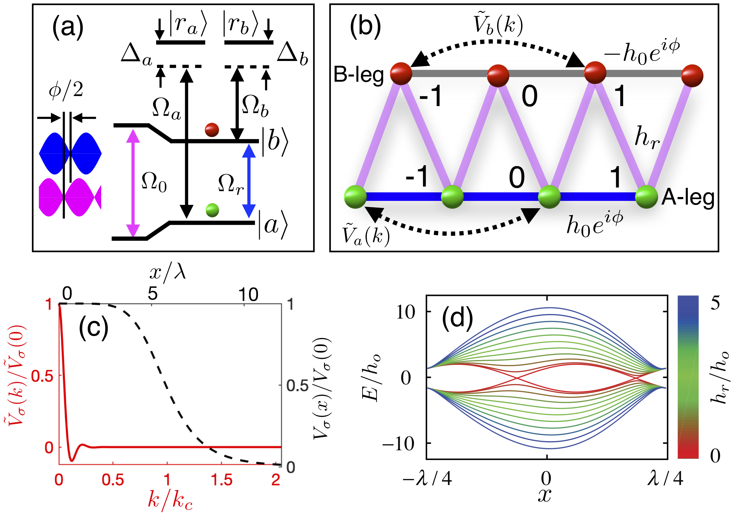
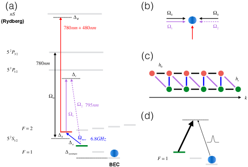
The two-leg Bose-Hubbard model— Collective atomic excitations stored in hyperfine states and [Fig. 1(a)] are created by an off-resonant and a resonant standing wave lasers along the -axis [with wave vector ( is the unit vector) and wave length ]. For small number of excitations, the spinwaves are described by free bosons Wang et al. (2015). By projecting the spinwave to momentum space with a characteristic momentum Wang et al. (2015), we obtain a ladder of A-leg and B-leg for the and states [Fig. 1(b)], respectively. The -th site of A-leg (B-leg) represents a collective state with wave vector []. When the standing wave lasers are phase mismatched [Fig. 1(a)], a synthetic magnetic field is generated Cai et al. (2019). This gives a nearest-neighbor hopping with complex amplitudes along and between the ladders, described by the Hamiltonian
where , and are the flux, intra- and inter-leg hopping amplitudes.
In our setting, state () is coupled to a Rydberg state () by an off-resonant laser. This induces a state-dependent two-body soft-core shape interaction , where and () are the dispersion coefficient and characteristic distance of the interaction potential, respectively. Their values can be engineered by tuning parameters of the dressing laser Henkel et al. (2010); Honer et al. (2010); Cinti et al. (2010); Li et al. (2012). The Hamiltonian for the interactions of the dressed state is,
where is the Fourier transformation of the corresponding interaction. decays rapidly with increasing as typically [Fig. 1(c)]. Finally the two-leg Bose-Hubbard Hamiltonian is given by with and to be the atomic density at site (momentum) and chemical potential in state . Details of the Hamiltonian can be found in the Supplemental Material (SM). In the following, we choose as the unit of the energy.
Symmetry and ground state phases in the interaction free case— The coupling Hamiltonian possesses [], [], and [], where , and are the time-reversal, chiral and translational symmetry operators. The chiral symmetry shows that currents after swapping the two states will remain the same if the flux is shifted simultaneously by , i.e. . The system does not preserve the time-reversal symmetry in general except when , where the ground state energy exhibits double degeneracy Cai et al. (2019), already leading to rich chiral phases (see examples in SM).
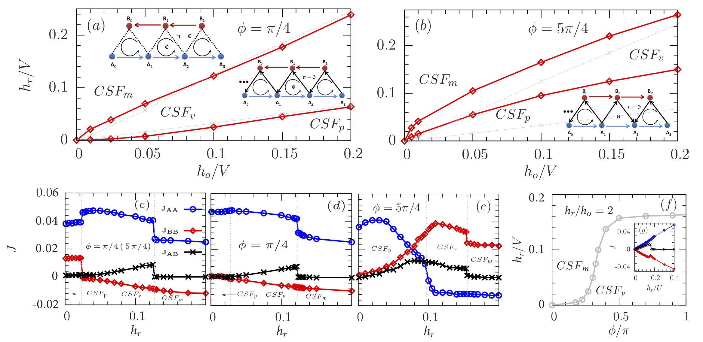
Solving exactly we obtain three types of band minima, i.e. a single minimum at real-space coordinate or , and two minima, as show in Fig. 1(d), analogous to spin-orbit coupling setup in real space Goldman et al. (2014) (the states and treated as spin and , respectively). The corresponding chiral phases are characterized by current for the bond and the leg , similar to the definition in real-space lattices Vasić et al. (2015); Plekhanov et al. (2018). As shown in Fig. 2, the ground state prefers a number of chiral superfluid phases (CSFs). When the inter-leg coupling is strong, currents along the ladders (edges) have opposite directions, i.e. and [Fig. 2(c)], denoted by phase (condensed into band minimum at ). When and are comparable, we have a different chiral superfluid phase ( condensed into band minimum at ) where currents on the ladders and rungs satisfy , and . The and phases are analogues of the Meissner and vortex phases of real-space ladder systems Mancini et al. (2015); Livi et al. (2016); Atala et al. (2014); Stuhl et al. (2015); Orignac and Giamarchi (2001); Boada et al. (2012); Petrescu and Le Hur (2013); Celi et al. (2014); Petrescu and Le Hur (2015); Tokuno and Georges (2014); Piraud et al. (2015); Greschner et al. (2016); Anisimovas et al. (2016); Calvanese Strinati et al. (2017); Price et al. (2017); Sundar et al. (2018); L. Barbiero and Goldman (2019).
When is further decreased, two band minima become degenerate [see Fig. 1(d)]. At the minima, currents on both ladders flow in the same direction, i.e. . This leads to a particularly interesting anti-chiral edge current (denoted by CSFp) in the system. Compared to real-space lattices Atala et al. (2014); Anisimovas et al. (2016), a fundamental difference of our scheme is the staggered magnetic flux, i.e. the flux of a plateau in the zigzag ladder is and its neighbor . The system then hosts asymmetric band structures in the regime , as shown in Fig. 1(d), with atoms in A- (B-) leg favoring the left (right) minimum [Fig. S2(b)]. As a result, the staggered flux induced asymmetric condensation of particles in each ladder changes directions of edge currents (a perturbative derivation for can be found in SM). As far as we know, this new quantum phase has not been studied in real-space lattice. Since the CSFp phase emerges in the limit , one could create this phase through an adiabatic manner. Starting with large and , one can adiabatically reduce (increase) () to enter the CSFp phase region while keeping () fixed. The anti-chiral edge current will be induced and saturate to a finite value even though .
Stable anti-chiral currents and excitation blockade by single Rydberg dressing. — In the single Rydberg dressing the B-leg is coupled to a Rydberg state (i.e. and ). We employ a bosonic dynamical mean-field calculation that captures both quantum fluctuations and strong correlations in a unified framework Li et al. (2011); Vasić et al. (2015); Plekhanov et al. (2018) (see SM for details). The reliability of this approach has been confirmed by a comparison with an unbiased quantum Monte Carlo simulation Anders et al. (2010).
Intuitively, one would expect currents are suppressed by the two-body interaction. On the contrary, the CSFs phases are stable against the dressed interaction [see Fig. 2(a) and (b)]. Actually, the two-body interaction breaks the chiral symmetry []. The broken symmetry is most apparent in the CSFp phase, where the phase region shrinks when [Fig. 2(a)] but expands when [Fig. 2(b)]. When , the two-body interaction reduces the energy separation between the two legs. As a result, both currents and are increased in the intermediate hopping regime. Here we observe a discontinuous phase transition in Fig. 2(c), and signatures of continues CSFp-CSFm phase transition by increasing [Fig. 2(d)(e)]. Furthermore, one can drive transitions between the CSF phases by varying the flux . One example can be found in Fig. 2(f), where the Meissner phase is driven to the vortex phase by changing the flux.
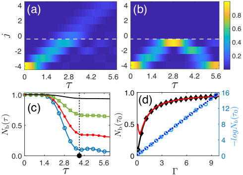
The two-body interaction plays a vital role in the dynamics. This is illustrated with a situation where initially two excitations at the first site of the A-leg (i.e. ) are prepared (see SM for details). When the atomic interaction is negligible, a large fraction of the excitation is transferred to the B-leg, as shown in Fig. 3(a). Turning on the interaction, the excitation probability in the B-leg is reduced apparently. A closer examination shows that the double occupation probability in the B-leg is significantly suppressed by the strong interaction. is the many-body state at time . This excitation suppression could be regarded as an interaction blockade in momentum space, analogue to the Rydberg blockade effect in real space Urban et al. (2009); Gaetan et al. (2009).
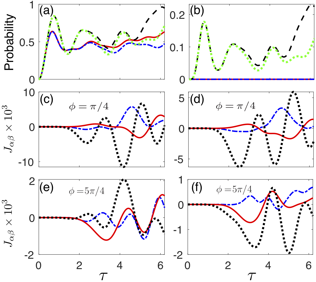
The dynamically generated currents show features of the ground state phases, though their strengths are suppressed by the interaction. For example, when the parameters are in the CSFv phase, for example, the currents counter-propagate on the two legs at the beginning of the evolution [Fig. 3(c)-(e)]. Surprisingly, the currents for along the legs become co-propagating when two-body interactions are important [Fig. 3(f)]. This behavior is similar to the currents found in the CSFp phase.
Sliding phases when both chains are laser dressed to Rydberg states.— A double Rydberg dressing is realized when the two legs are coupled to two different Rydberg states. For energetically close Rydberg states, this leads to similar dressed potentials for the two legs. Without loss of generality, we focus on the case with in the following.
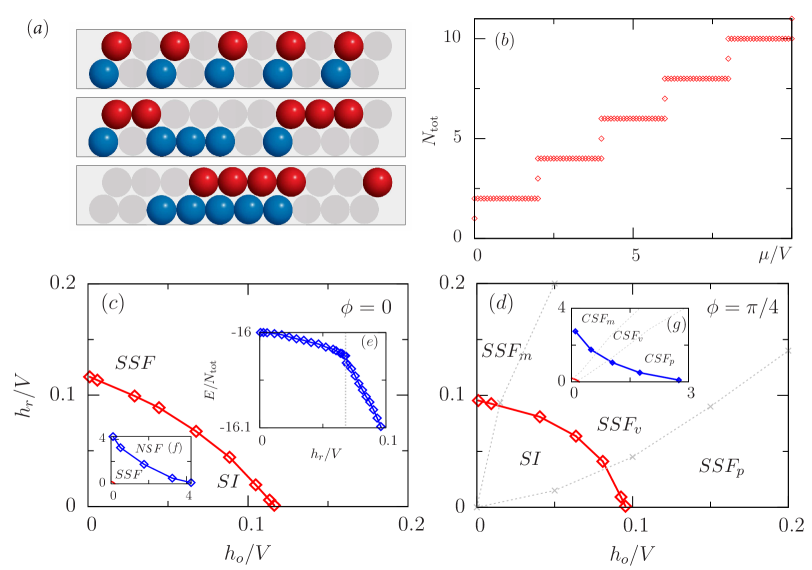
Without hopping (), the ground state is an unusual insulating state with a high degree of degeneracy , where is the binomial coefficient, and denote the number of particles, and and the lattice number in A- and B-legs, respectively. Its energy [ dominates when ] depends on the total number of particles but not their distributions in the momentum-space ladder, i.e. changing their locations in the corresponding leg costs no energy. In Fig. 4(a), we illustrate this phase with an example of five bosons along each leg. We attribute this phase as a sliding insulating phase (SI), analogous to long-sought sliding superfluid phase Choi and Doniach (1985); Granato and Kosterlitz (1986); O’Hern and Lubensky (1998); O’Hern et al. (1999); Pekker et al. (2010); Niu et al. (2018). The underlying physics of the emergent SI studied here is a result of momentum-space Rydberg coupling (all sites equally coupled) from the long-range real-space Rydberg interaction. Varying the chemical potential, the ground state forms Devil’s staircase structures with non-integer filling [Fig. 4(b)], which breaks the lattice translational symmetry.
Turning on the hopping, the sliding insulating phase is stable in the low hopping regime (), as shown in the phase diagram Fig. 4(c) and (d) (detailed discussions for finite hopping shown in SM). For larger hopping amplitudes, density fluctuations are stronger and a sliding superfluity phase (SSF) appears. The SI-SSF phase transition can be determined by examining the ground state energy [Fig. 4(e)]. Note that the SSF breaks both lattice translational and gauge symmetries, and therefore can be considered as a sliding supersolid phase. In the weakly interacting regime (), kinetic energy dominates and normal superfluid (NSF) appears [Fig. 4(f)(g)]. In the presence of external magnetic flux, the chiral symmetry is broken, i.e. nonzero local currents are found in the sliding phases. In the weakly interacting limit, normal chiral superfluid phases emerge in the ground state.
Conclusion— A momentum-space lattice model suitable for investigating topological physics and correlated many-body dynamics is proposed. Using single and double Rydberg dressing, the ground state exhibits a series of exotic phases, including anti-chiral edge currents, sliding insulating and superfluid states. Strongly correlated dynamics, such as the state dependent excitation blockade, is found due to the competition between the chirality and strong Rydberg interactions. Compared to schemes based on superradiant Dicke states characterized by steady states Wang et al. (2015); Chen et al. (2018); Cai et al. (2019), our setting permits to explore correlated chiral phenomena both in and out of equilibrium coherently. Compared to real-space magnetic ladder system, our system is essentially a spin-orbit coupling setup in momentum space, and supports three distinctive chiral broken phases.
Our study paves new routes towards the study of chirality with interacting spinwaves in higher dimensions and external driving. In frustrated lattices (e.g. honeycomb lattices), emergent quantum topological dynamics can be investigated in a Hamiltonian system, e.g., by quenching the system from a trivial to topological state. When dissipation is introduced, this opens opportunities to uncover stability of edge modes, as well as to explore competing dynamics between atomic interactions and dissipation in an open quantum system (example of quantum Zeno effect is discussed in SM.).
I Acknowledgements
Authors would like to thank helpful discussions with Jing Zhang, Yinghai Wu, XiongJun Liu, and Tao Shi. This work is supported by the National Natural Science Foundation of China under Grants No. 11304386 and No. 11774428 (Y. L.), by the UKIERI-UGC Thematic Partnership No. IND/CONT/G/16-17/73, EPSRC Grant No. EP/M014266/1 and EP/R04340X/1 (W. L.), and by National Natural Science Foundation of China (No. 11874322), the National Key Research and Development Program of China (Grant No. 2018YFA0307200) (D. W.). The work was carried out at National Supercomputer Center in Tianjin, and the calculations were performed on TianHe-1A.
Supplementary Material
S-2 Extended Bose-Hubbard model in momentum space
S-2.1 The Hamiltonian in momentum space
Here we consider N three-level atoms, i.e. ground state , another ground state and Rydberg dressed state , where is the position of the th atom with random distribution. The atoms are initially prepared in the ground state . A standing wave laser couples the atomic and states with vectors . In the rotating wave approximation, the Hamiltonian reads
| (S1) |
where and is the dispersion coefficient and characteristic distance of the soft-core shape interaction, respectively Henkel et al. (2010); Honer et al. (2010); Cinti et al. (2010); Li et al. (2012). Collective atomic excitation operators in momentum space are introduced as
| (S2) |
| (S3) |
We transform the Hamiltonian from position space to momentum space via
| (S4) |
| (S5) |
The total Hamiltonian in momentum space can be written as
| (S6) | |||||
where , and the transformation is valid for many excitations if the excitation number is much less than the atom number Wang et al. (2015).
Here, if we switch on another far-tuned standing wave lasers and couple the state to another Rydberg state, then an extra interaction term appears due to the AC Stark shifts Cai et al. (2019). The total Hamiltonian is given by:
| (S7) | |||||
S-3 bosonic dynamical mean-field theory
To investigate ground states of bosonic gases loaded into momentum-space lattices, described by Eq. (S7), we establish a bosonic version of dynamical mean-field theory (BDMFT) on the ladder system with , where is the number of neighbors connected by hopping terms. As in fermionic dynamical mean field theory, the main idea of the BDMFT approach is to map the quantum lattice problem with many degrees of freedom onto a single site - ”impurity site” - coupled self-consistently to a noninteracting bath Georges et al. (1996). The dynamics at the impurity site can thus be thought of as the interaction (hybridization) of this site with the bath. Note here that this method is exact for infinite dimensions, and is a reasonable approximation for neighbors . In the noninteracting limit, the problem is trivially solvable in all dimensions, all correlation functions factorize and the method becomes exactly Byczuk and Vollhardt (2008).
S-3.1 BDMFT equations
In deriving the effective action, we consider the limit of a high but finite dimensional optical lattice, and use the cavity method Georges et al. (1996) to derive self-consistency equations within BDMFT. In the following, we use the notation for the hopping amplitude between sites and , and define creation field operator for the state [] to shorten Ham. (S7). And then the effective action of the impurity site up to subleading order in is then expressed in the standard way Georges et al. (1996); Byczuk and Vollhardt (2008), which is described by:
with Weiss Green’s function
| (S12) | |||
| (S15) |
and superfluid order parameter
| (S16) |
Here, we have defined the the diagonal and off-diagonal parts of the connected Green’s functions
| (S17) | |||||
| (S18) |
where denotes the expectation value in the cavity system (without the impurity site).
To find a solver for the effective action, we return back to the Hamiltonian representation and find that the local Hamiltonian is given by a bosonic Anderson impurity model.
| (S19) |
where the chemical potential and interaction term are directly inherited from the Hubbard Hamiltonian. The bath of condensed bosons is represented by the Gutzwiller term with superfluid order parameters . The bath of normal bosons is described by a finite number of orbitals with creation operators and energies , where these orbitals are coupled to the impurity via normal-hopping amplitudes and anomalous-hopping amplitudes . The anomalous hopping terms are needed to generate the off-diagonal elements of the hybridization function.
The Anderson Hamiltonian can be implemented in the Fock basis, and the corresponding solution can be obtained by exact diagonalization of BDMFT Georges et al. (1996). After diagonalization, the local Green’s function, which includes all the information about the bath, can be obtained from the eigenstates and eigenenergies in the Lehmann-representation
| (S20) | |||||
| (S21) |
Integrating out the orbitals leads to the same effective action as in Eq. (S-3.1), if the following identification is made
| (S22) |
where , , and means summation only over the nearest neighbors of the ”impurity site”.
In next step, we make the approximation that the lattice self-energy coincides with the impurity self-energy , which is obtained from the local Dyson equation
| (S23) |
The real-space Dyson equation takes the following form:
| (S24) |
Here, the self-consistency loop is closed by Eq. (S20)-(S24), and this self-consistency loop is repeated until the desired accuracy for values of parameters , and and superfluid order parameter is obtained.
S-4 Ground state phase diagram for
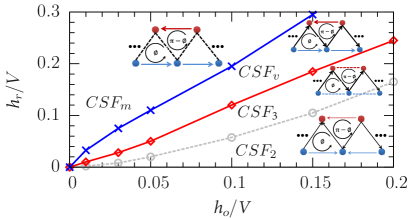
Without two-body interactions, or with single Rydberg dressing, there are two special case for the flux and . For the case , the phenomena are trivial, and the system does not support edge currents in the absence (presence) of Rydberg long-range interactions. For the case , the band structure of the lattice system is actually a double-valley well with two degenerate band minima connected by time-reversal symmetry, indicating that more ground states appear in the case. Here we choose the parameters: the filling factor ( being the lattice size) and . We observe there are four stable phases in the diagram with different types of ground state edge currents, including CSF2 and CSF3 with currents on the rung but with a suppressed global current on both ladders with and , CSFm with currents only on the ladders, and CSFv with currents on both ladders and rungs. The physical reason of the suppressed edge currents of the CSF2 and CSF3 phases is that, and with , being the filling at site , and condensing at and , respectively.
S-5 Density distribution in real space and momentum space with single Rydberg dressing
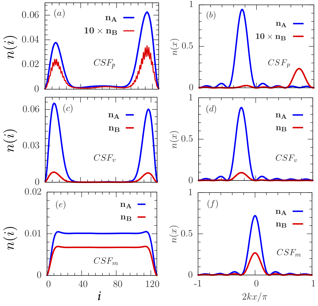
In the main text, we identified three phases in the case of single Rydberg dressing. The density distributions in momentum and real space are vastly different in the three phases. Here we will show both real-space and momentum-space density distributions in these phases, which might be observed directly through time-of-flight experiment. In the Meissner phase, the size of the vortex is infinite and the density is uniform in the momentum-space lattice. On the other hand, in the CSFp and CSFv phases, the system exhibits vortex structures, where the densities are distributed inhomogeneously and the vortexes are separated into different regions (the averaged inter-leg current and for the CSFp and CSFv phases, respectively).
Actually, we have observed that there are three different kinds of band structures in the noninteracting system, as shown in Fig. 1(d), where band minima are localized at zero (CSFm), finite-value (CSFv), and doubly degenerate points (CSFp) in real space Cai et al. (2019). The interacting system also supports three types of condensation in real space, and the resulting phenomena are that, in the CSFp phase, the maximal density for the and states, localized at and , respectively, separates by about [ and with , as shown in Fig. S2(b) for and , and more discussions on the anti-chiral current are shown in the next section], and in the CSFv phase, peak positions of the two states are identical in real space condensing at nonzero value. In the CSFm phase, however, the maximal value of the density in the two states is centered at in real space. This indicates that we can directly identify the CSFp phase through the real-space distribution.
S-6 CSFp phase without two-body interactions
When the two-body interaction is vanishing, the Hamiltonian of an ensemble of atoms in real space is given by
| (S25) |
where is the index of atoms. The eigenvalues of the Hamiltonian are .
In the limit the two eigenvalues as a function of will cross at . We can also find that when (for state ) and (for state ), the eigenenergies are local minimal. The current and are zero in this limit.
Now focusing on the case and turning on the coupling between the two states, the two local minimal points are coupled. When , the two local minimal points are still nearly degenerate. The minimal points are shifted slightly with respect to and . We can expand the lower branch of the eigenenergy around up to second order and find the shifts, and . The current . Similarly, we find that . Here because the state is weakly occupied in the ground state, due to small . This explains the results shown in the main text.
S-7 Sliding phases in the strongly interacting regime
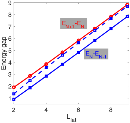
The unique properties of the sliding phase can be understood by considering a single chain. In the following we will consider the A-leg with excitation from the atomic hyperfine ground state as an example. In the momentum space, all the excitations are coupled by the infinite long-range Rydberg interactions. The interaction energy regardless of the particle distribution. The energy gap by adding one particle and removing one particle depends on particle numbers linearly, where denotes the ground state energy of the system. This is approximately valid even in the presence of a weak hopping. To verify this, we have carried out exact diagonalization (ED) calculations for unit filling . To calculate the gap, we have considered system size up to and , whose Hilbert space is 43758. Our numerical results show that the energy gap is indeed proportional to particle numbers (see Fig. S3). On the other hand, the ratio of the two gaps when the hopping vanishes. The numerical simulation shows that the ratio is approximately correct (Fig. S3). The deviation in the numerical calculation is due to the finite size effect.
Moreover, we can understand the existence of the sliding phase from the relative bandwidth of the system, i.e. the ratio between the hopping and interaction energy. First, the maximal value of the hopping energy is , corresponding to a configuration where and atoms locate at two neighboring sites. In the thermodynamic limit, the relative bandwidth is estimated as
| (S26) |
This power decay indicates that the relative bandwidth vanishes for the Rydberg-dressed system in the thermodynamic limit. As a result, a sliding phase emerges in the strongly interacting limit. As a comparison, we note that the relative bandwidth in the Mott insulator state of the Bose-Hubbard model, described by , is with filling (i.e. the mean number of atoms in a site). The corresponding bandwidth is constant in the thermodynamic limit.

It becomes difficult to carry out ED calculation for larger systems, such as two coupled chains with larger . Here we calculate energy distributions for different numerical simulations via the dynamical mean-field theory. The ground state energies, with different density distributions, localize in a small region (compared to hopping amplitudes), indicating the sliding nature of the quantum many-body states at finite hopping amplitudes, as shown Fig. S4. The broadening of the spectra is largely caused by the kinetic energy of different configurations of the finite-size system [see Fig. S4(b), (c), (e) and (f)]. As examples, we also show density distributions in momentum space from two different numerical simulations [Fig. S4(b) and (c) in SI, and Fig. S4(e) and (f) in SSF region] but with the same parameters. In different simulations, the particles distribute randomly in each ladder, as shown in Fig. S4(b)(c) and (e)(f). Experimental observation of such distribution could be a direct evidence of the sliding phase.
S-8 Quantum Zero dynamics with effective decay
When the long-lived hyperfine states are replaced with low-lying decay states, we realize a superradiance lattice Wang et al. (2015), or incorporate an effective decay in the present setup. To highlight the collective decay, we study dissipative dynamics of the A-leg solely and turn off the dressing laser. It could be realized by coupling the level with a strong classical field off-resonantly. Spontaneous Raman process happens in a rare probability, which depends on the detuning. It’s a reversal process of the state initialization as we mentioned above.
Without two-body interactions, we will study a single excitation in the A-leg, whose dynamics is now described by a master equation
| (S27) |
where . are decay rate of the -th site. Propagation of the spinwave depends on hopping and decay rate . The latter is site (momentum) dependent for a superradiance lattice. With this consideration, only for phase matched spinwave components Svidzinsky and Chang (2008), i.e. at sites with index and [see Fig. 1(b)].
We consider a single excitation initially occupies the state and propagates to the middle of the lattice. One typically expects that the propagation is coherent away from the central sites, and becomes dissipative once approaching to the decaying sites. This is true when the decay rate is small, where a large fraction of the population will be lost [Fig. S5(a)]. The dynamics changes qualitatively when is large, where the population is largely reflected at the zeroth site [Fig. S5(b)(c)].
We attribute the reflection to the quantum Zeno effect Scully and Zubairy (1997). Stronger decay behaves similar to a frequent measurement of occupations in the zeroth site. It prohibits the occupation of its neighboring sites from hopping to the initially not occupied center sites. As a result, the loss occurs at an effective, smaller rate Daley (2014). To illustrate this, we consider the simplest model which contains only the two sites with index and . The initial state is with and (the subscript indicates the site index.). This state couples to the state , which will decay at a rate . The effective decay rate can be estimated through analyzing the non-Hermitian Hamiltonian Daley (2014), , where the coupling and diagonal Hamiltonian . The energy of the initial state in the presence of the coupling can be solved through the second order perturbation Daley (2014)
| (S28) |
The initial state evolves according to . Hence the remaining probability of the initial state is
| (S29) |
The initial state decays at an effective rate , which decreases with increasing .
We numerically calculate the remaining population as a function of at time , when the reflection occurs. As shown in Fig. S5(d), the effective decay rate is linearly proportional to , confirming the analytical prediction.
S-9 Experimental proposal for realizing strongly correlated phenomena
Chiral edge states can be realized in momentum space, either using mechanical momentum states of cold atoms Gadway (2015); An et al. (2017, 2018a, 2018b); Meier et al. (2018), or collective excitation formed by collective excitations of electronic states Scully et al. (2006). A unique advantage of the latter is that thermal resistant edge states can be probed, since the momentum-space lattice Wang et al. (2015); Chen et al. (2018) of collective atomic excitations is immune to the motional entropy of atoms. The first proof-of-principle experiment has demonstrated chiral edge currents at the room temperature recently Cai et al. (2019). However, electronic excited states suffer from fast spontaneous decay, inducing a steady state in the pump-dissipative system and destroying the nature of the system. A clean quantum system in the momentum-space lattice in the presence of strong interactions is required to simulate strongly correlated phenomena.
S-9.1 Realization for the Hamiltonian (1) without dissipation
We can get rid of the radiative dissipation by selecting three hyperfine spin states in ground levels of with being , being , and being . The atomic level scheme and the configuration of the coupling beams are plotted in Fig. S6(a)(b). The spin states are split by a bias magnetic field. The inter-leg coupling in purple is realized by Raman interaction which composed by the two fields around D1 line (in purple), while the one in blue is realized by a 6.8GHz microwave field. Since microwave field transfers negligible momentum, the MSL is slightly tilted in momentum space, as shown in Fig. S6(c). The intra-leg coupling is implemented by the standing waves around D2 line, whose frequency is set in the middle point between and levels to introduce the phase shift between the intra-leg couplings of A- and B-legs. The phase in Ham. (1) can be controlled by manipulating the phase of the microwave and optical driving fields. Note here that, the small difference between the wave vectors of the standing wave is negligible. In the low-excitation regime, these atomic spinwave states are described by bosons Fleischhauer and Lukin (2000).
Here we choose Rydberg 60 state as an example, whose lifetime is 102 s. With the detuning MHz and Rabi frequency MHz of the dressing laser, the effective lifetime in the Rydberg dressed state is 2.9 ms. We obtain m and kHz. This large soft-core radius leads to a short-range interaction in momentum space, as it is far larger than the wavelength of the standing wave laser ( nm). The inter- and intra-leg coupling strengths and can vary in a large parameter regimes. For example, we choose the parameters being the Zeeman splitting between and , being the detunings [see details in Fig. S6(a)], being the Rabi frequencies of optical fields with , and being the effective Rabi frequency of the microwave field. The corresponding and are (, with being the recoil energy), which are larger enough to observe coherent dynamics in microsecond timescale.
S-9.2 Loading the excitations and measurement
To observe the dynamics in MSL, we need to initialize excitations in the A-leg with a post-selection process. The BEC is prepared in ground state before turning on the Ham. (S7). Then we apply a strong classical field (thick) and a single photon (thin) in Fig. S6(d), forming a Raman coupling. When the single photon is not observed by a detector on its incident direction, we know one excitation is loaded in level Scully et al. (2006). Since the coherent time of level is long enough, we can repeat the process twice to prepare the two-excitation state in zeroth site in A-leg. For the Zeno dynamics, we need to prepare a single excitation on the th site in A-leg and introduce an effective decay to the zeroth one (see more details in the next subsection). After the single excitation is loaded into the zeroth site, we can apply two -pulses of blue and purple couplings in a sequence. Such a pulse pair transport the excitation from the zeroth site to the first site in the A-leg. We can repeat the process for times to finish the initialization.Wang and Scully (2014).
We can also pump the excitation to the MSL when the Hamiltonian is on. By tuning the frequency of the pumping microwave field to the energy of the ground state in MSL, we can excite a specific state with high fidelity since the state width is very narrow. To prepare the total excitations , the pulse area of the pumping microwave field is roughly estimated as , where is the effective Rabi frequency of the pumping microwave field, is the collective enhancement of atoms, and is the pulse duration.
By measuring the probability distribution of the - and -level atoms in momentum space via time of flight imaging, we can obtain the distribution of the excitation in MSL, which is expected to show the strongly correlated phenomena, e.g. ground state chiral current Atala et al. (2014), excitation blockade, and Zeno dynamics.
References
- Klitzing et al. (1980) K. V. Klitzing, G. Dorda, and M. Pepper, Physical Review Letters 45, 494 (1980).
- Thouless et al. (1982) D. J. Thouless, M. Kohmoto, M. P. Nightingale, and M. den Nijs, Phys. Rev. Lett. 49, 405 (1982).
- Hasan and Kane (2010) M. Z. Hasan and C. L. Kane, Reviews of Modern Physics 82, 3045 (2010).
- Senthil (2015) T. Senthil, Annual Review of Condensed Matter Physics 6, 299 (2015).
- Sinova et al. (2015) J. Sinova, S. O. Valenzuela, J. Wunderlich, C. H. Back, and T. Jungwirth, Reviews of Modern Physics 87, 1213 (2015).
- Hansson et al. (2017) T. H. Hansson, M. Hermanns, S. H. Simon, and S. F. Viefers, Reviews of Modern Physics 89, 025005 (2017).
- Bloch et al. (2008) I. Bloch, J. Dalibard, and W. Zwerger, Rev. Mod. Phys. 80, 885 (2008).
- Lewenstein et al. (2012) M. Lewenstein, A. Sanpera, and V. Ahufinger, Ultracold Atoms in Optical Lattices: Simulating quantum many-body systems (Oxford University Press, 2012).
- Bromley et al. (2018) S. L. Bromley, S. Kolkowitz, T. Bothwell, D. Kedar, A. Safavi-Naini, M. L. Wall, C. Salomon, A. M. Rey, and J. Ye, Nature Physics 14, 399 (2018).
- Goldman et al. (2016) N. Goldman, J. C. Budich, and P. Zoller, Nature Physics 12, 639 (2016).
- Dalibard et al. (2011) J. Dalibard, F. Gerbier, G. Juzeliūnas, and P. Öhberg, Rev. Mod. Phys. 83, 1523 (2011).
- Goldman et al. (2014) N. Goldman, G. Juzeliūnas, P. Öhberg, and I. B. Spielman, Reports on Progress in Physics 77, 126401 (2014).
- Cooper et al. (2019) N. R. Cooper, J. Dalibard, and I. B. Spielman, Rev. Mod. Phys. 91, 015005 (2019).
- Lin et al. (2009) Y.-J. Lin, R. L. Compton, K. Jiménez-García, J. V. Porto, and I. B. Spielman, Nature 462, 628 (2009).
- Lin et al. (2010) Y. Lin, R. L. Compton, K. Jiménez-García, W. D. Phillips, J. V. Porto, and I. B. Spielman, Nature Physics 7, 531 (2010).
- Mancini et al. (2015) M. Mancini, G. Pagano, G. Cappellini, L. Livi, M. Rider, J. Catani, C. Sias, P. Zoller, M. Inguscio, and M. Dalmonte, Science 349, 1510 (2015).
- Livi et al. (2016) L. F. Livi, G. Cappellini, M. Diem, L. Franchi, C. Clivati, M. Frittelli, F. Levi, D. Calonico, J. Catani, M. Inguscio, and L. Fallani, Phys. Rev. Lett. 117, 220401 (2016).
- Atala et al. (2014) M. Atala, M. Aidelsburger, M. Lohse, J. Barreiro, B. Paredes, and I. Bloch, Nature Physics 10, 588 (2014).
- Stuhl et al. (2015) B. K. Stuhl, H.-I. Lu, L. M. Aycock, D. Genkina, and I. B. Spielman, Science 349, 1514 (2015).
- Kang et al. (2018) J. H. Kang, J. H. Han, and Y. Shin, Phys. Rev. Lett. 121, 150403 (2018).
- Aidelsburger et al. (2011) M. Aidelsburger, M. Atala, S. Nascimbène, S. Trotzky, Y.-A. Chen, and I. Bloch, Physical Review Letters 107, 487 (2011).
- Struck et al. (2012) J. Struck, C. Ölschläger, M. Weinberg, P. Hauke, J. Simonet, A. Eckardt, M. Lewenstein, K. Sengstock, and P. Windpassinger, Phys. Rev. Lett. 108, 225304 (2012).
- Aidelsburger et al. (2013) M. Aidelsburger, M. Atala, M. Lohse, J. T. Barreiro, B. Paredes, and I. Bloch, Phys. Rev. Lett. 111, 185301 (2013).
- Hirokazu et al. (2013) M. Hirokazu, G. A. Siviloglou, C. J. Kennedy, B. William Cody, and K. Wolfgang, Physical Review Letters 111, 185302 (2013).
- Gregor et al. (2014) J. Gregor, M. Michael, D. Rémi, L. Martin, U. Thomas, G. Daniel, and E. Tilman, Nature 515, 237 (2014).
- Kennedy et al. (2015) C. J. Kennedy, W. C. Burton, W. C. Chung, and W. Ketterle, Nature Physics 11, 1106 (2015).
- Fläschner et al. (2016) N. Fläschner, B. S. Rem, M. Tarnowski, D. Vogel, D.-S. Lühmann, K. Sengstock, and C. Weitenberg, Science 352, 1091 (2016).
- Asteria et al. (2019) L. Asteria, D. T. Tran, T. Ozawa, M. Tarnowski, B. S. Rem, N. Fläschner, K. Sengstock, B. Goldman, and C. Weitenberg, Nature Physics 15, 449 (2019).
- Wall et al. (2016) M. L. Wall, A. P. Koller, S. Li, X. Zhang, N. R. Cooper, J. Ye, and A. M. Rey, Physical Review Letters 116, 035301 (2016).
- Zhou et al. (2017) X. Zhou, J.-S. Pan, Z.-X. Liu, W. Zhang, W. Yi, G. Chen, and S. Jia, Phys. Rev. Lett. 119, 185701 (2017).
- Kolkowitz et al. (2016) S. Kolkowitz, S. L. Bromley, T. Bothwell, M. L. Wall, G. E. Marti, A. P. Koller, X. Zhang, A. M. Rey, and J. Ye, Nature 542, 66 (2016).
- Tai et al. (2017) M. E. Tai, A. Lukin, M. Rispoli, R. Schittko, T. Menke, B. Dan, P. M. Preiss, F. Grusdt, A. M. Kaufman, and M. Greiner, Nature 546, 519 (2017).
- He et al. (2019) P. He, M. A. Perlin, S. R. Muleady, R. J. Lewis-Swan, R. B. Hutson, J. Ye, and A. M. Rey, 1904.07866 (2019).
- Saffman et al. (2010) M. Saffman, T. G. Walker, and K. Mølmer, Rev. Mod. Phys. 82, 2313 (2010).
- Labuhn et al. (2016) H. Labuhn, D. Barredo, S. Ravets, S. De Léséleuc, T. Macrì, T. Lahaye, and A. Browaeys, Nature 534, 667 (2016).
- Levine et al. (2018) H. Levine, A. Keesling, A. Omran, H. Bernien, S. Schwartz, A. S. Zibrov, M. Endres, M. Greiner, V. Vuletić, and M. D. Lukin, Phys. Rev. Lett. 121, 123603 (2018).
- Omran et al. (2019) A. Omran, H. Levine, A. Keesling, G. Semeghini, T. T. Wang, S. Ebadi, H. Bernien, A. S. Zibrov, H. Pichler, S. Choi, et al., Science 365, 570 (2019).
- de Léséleuc et al. (2019) S. de Léséleuc, V. Lienhard, P. Scholl, D. Barredo, S. Weber, N. Lang, H. P. Büchler, T. Lahaye, and A. Browaeys, Science 365, 775 (2019).
- Celi et al. (2019) A. Celi, B. Vermersch, O. Viyuela, H. Pichler, M. D. Lukin, and P. Zoller, arXiv preprint arXiv:1907.03311 (2019).
- Bouchoule and Mølmer (2002) I. Bouchoule and K. Mølmer, Phys. Rev. A 65, 041803 (2002).
- Pupillo et al. (2010) G. Pupillo, A. Micheli, M. Boninsegni, I. Lesanovsky, and P. Zoller, Phys. Rev. Lett. 104, 223002 (2010).
- Honer et al. (2010) J. Honer, H. Weimer, T. Pfau, and H. P. Büchler, Phys. Rev. Lett. 105, 160404 (2010).
- Cinti et al. (2010) F. Cinti, P. Jain, M. Boninsegni, A. Micheli, P. Zoller, and G. Pupillo, Phys. Rev. Lett. 105, 135301 (2010).
- Li et al. (2012) W. Li, L. Hamadeh, and I. Lesanovsky, Phys. Rev. A 85, 053615 (2012).
- Henkel et al. (2010) N. Henkel, R. Nath, and T. Pohl, Phys. Rev. Lett. 104, 195302 (2010).
- Bounds et al. (2018) A. D. Bounds, N. C. Jackson, R. K. Hanley, R. Faoro, E. M. Bridge, P. Huillery, and M. P. A. Jones, Phys. Rev. Lett. 120, 183401 (2018).
- Jau et al. (2016) Y.-Y. Jau, A. M. Hankin, T. Keating, I. H. Deutsch, and G. W. Biedermann, Nature Physics 12, 71 (2016).
- Zeiher et al. (2016) J. Zeiher, R. Van Bijnen, P. Schauß, S. Hild, J.-y. Choi, T. Pohl, I. Bloch, and C. Gross, Nature Physics 12, 1095 (2016).
- Wang et al. (2015) D.-W. Wang, R.-B. Liu, S.-Y. Zhu, and M. O. Scully, Phys. Rev. Lett. 114, 043602 (2015).
- Cai et al. (2019) H. Cai, J. Liu, J. Wu, Y. He, S.-Y. Zhu, J.-X. Zhang, and D.-W. Wang, Phys. Rev. Lett. 122, 023601 (2019).
- (51) We consider the system with lattice sites up to to verify the finite-size effects on phase diagrams .
- Vasić et al. (2015) I. Vasić, A. Petrescu, K. Le Hur, and W. Hofstetter, Phys. Rev. B 91, 094502 (2015).
- Plekhanov et al. (2018) K. Plekhanov, I. Vasić, A. Petrescu, R. Nirwan, G. Roux, W. Hofstetter, and K. Le Hur, Phys. Rev. Lett. 120, 157201 (2018).
- Orignac and Giamarchi (2001) E. Orignac and T. Giamarchi, Phys. Rev. B 64, 144515 (2001).
- Boada et al. (2012) O. Boada, A. Celi, J. I. Latorre, and M. Lewenstein, Phys. Rev. Lett. 108, 133001 (2012).
- Petrescu and Le Hur (2013) A. Petrescu and K. Le Hur, Phys. Rev. Lett. 111, 150601 (2013).
- Celi et al. (2014) A. Celi, P. Massignan, J. Ruseckas, N. Goldman, I. B. Spielman, G. Juzeliūnas, and M. Lewenstein, Phys. Rev. Lett. 112, 043001 (2014).
- Petrescu and Le Hur (2015) A. Petrescu and K. Le Hur, Phys. Rev. B 91, 054520 (2015).
- Tokuno and Georges (2014) A. Tokuno and A. Georges, New Journal of Physics 16, 073005 (2014).
- Piraud et al. (2015) M. Piraud, F. Heidrich-Meisner, I. P. McCulloch, S. Greschner, T. Vekua, and U. Schollwöck, Phys. Rev. B 91, 140406 (2015).
- Greschner et al. (2016) S. Greschner, M. Piraud, F. Heidrich-Meisner, I. P. McCulloch, U. Schollwöck, and T. Vekua, Phys. Rev. A 94, 063628 (2016).
- Anisimovas et al. (2016) E. Anisimovas, M. Račiūnas, C. Sträter, A. Eckardt, I. B. Spielman, and G. Juzeliūnas, Phys. Rev. A 94, 063632 (2016).
- Calvanese Strinati et al. (2017) M. Calvanese Strinati, E. Cornfeld, D. Rossini, S. Barbarino, M. Dalmonte, R. Fazio, E. Sela, and L. Mazza, Phys. Rev. X 7, 021033 (2017).
- Price et al. (2017) H. M. Price, T. Ozawa, and N. Goldman, Phys. Rev. A 95, 023607 (2017).
- Sundar et al. (2018) B. Sundar, B. Gadway, and K. R. Hazzard, Scientific reports 8, 3422 (2018).
- L. Barbiero and Goldman (2019) S. N. L. Barbiero, L. Chomaz and N. Goldman, arXiv preprint arXiv:1907.10555 (2019).
- Li et al. (2011) Y.-Q. Li, M. R. Bakhtiari, L. He, and W. Hofstetter, Phys. Rev. B 84, 144411 (2011).
- Anders et al. (2010) P. Anders, E. Gull, L. Pollet, M. Troyer, and P. Werner, Phys. Rev. Lett. 105, 096402 (2010).
- Urban et al. (2009) E. Urban, T. A. Johnson, T. Henage, L. Isenhower, D. D. Yavuz, T. G. Walker, and M. Saffman, Nat. Phys. 5, 110 (2009).
- Gaetan et al. (2009) A. Gaetan, Y. Miroshnychenko, T. Wilk, A. Chotia, M. Viteau, D. Comparat, P. Pillet, A. Browaeys, and P. Grangier, Nat. Phys. 5, 115 (2009).
- Choi and Doniach (1985) M. Y. Choi and S. Doniach, Phys. Rev. B 31, 4516 (1985).
- Granato and Kosterlitz (1986) E. Granato and J. M. Kosterlitz, Phys. Rev. B 33, 4767 (1986).
- O’Hern and Lubensky (1998) C. S. O’Hern and T. C. Lubensky, Phys. Rev. Lett. 80, 4345 (1998).
- O’Hern et al. (1999) C. S. O’Hern, T. C. Lubensky, and J. Toner, Phys. Rev. Lett. 83, 2745 (1999).
- Pekker et al. (2010) D. Pekker, G. Refael, and E. Demler, Phys. Rev. Lett. 105, 085302 (2010).
- Niu et al. (2018) L. Niu, S. Jin, X. Chen, X. Li, and X. Zhou, Phys. Rev. Lett. 121 (2018).
- Chen et al. (2018) L. Chen, P. Wang, Z. Meng, L. Huang, H. Cai, D.-W. Wang, S.-Y. Zhu, and J. Zhang, Phys. Rev. Lett. 120, 193601 (2018).
- Georges et al. (1996) A. Georges, G. Kotliar, W. Krauth, and M. J. Rozenberg, Rev. Mod. Phys. 68, 13 (1996).
- Byczuk and Vollhardt (2008) K. Byczuk and D. Vollhardt, Phys. Rev. B 77, 235106 (2008).
- Svidzinsky and Chang (2008) A. Svidzinsky and J.-T. Chang, Phys. Rev. A 77, 043833 (2008).
- Scully and Zubairy (1997) M. O. Scully and M. S. Zubairy, Quantum Optics, 1st ed. (Cambridge University Press, 1997).
- Daley (2014) A. J. Daley, arXiv:1405.6694 [cond-mat, physics:quant-ph] (2014).
- Gadway (2015) B. Gadway, Phys. Rev. A 92, 043606 (2015).
- An et al. (2017) F. A. An, E. J. Meier, and B. Gadway, Science advances 3, e1602685 (2017).
- An et al. (2018a) F. A. An, E. J. Meier, J. Ang’ong’a, and B. Gadway, Phys. Rev. Lett. 120, 040407 (2018a).
- An et al. (2018b) F. A. An, E. J. Meier, and B. Gadway, Phys. Rev. X 8, 031045 (2018b).
- Meier et al. (2018) E. J. Meier, F. A. An, A. Dauphin, M. Maffei, P. Massignan, T. L. Hughes, and B. Gadway, Science 362, 929 (2018).
- Scully et al. (2006) M. O. Scully, E. S. Fry, C. H. R. Ooi, and K. Wódkiewicz, Phys. Rev. Lett. 96, 010501 (2006).
- Fleischhauer and Lukin (2000) M. Fleischhauer and M. D. Lukin, Phys. Rev. Lett. 84, 5094 (2000).
- Wang and Scully (2014) D.-W. Wang and M. O. Scully, Physical Review Letters 113, 083601 (2014).