Subword Language Model for Query Auto-Completion

Abstract

Current neural query auto-completion (QAC) systems rely on character-level language models, but they slow down when queries are long. We present how to utilize subword language models for the fast and accurate generation of query completion candidates. Representing queries with subwords shorten a decoding length significantly. To deal with issues coming from introducing subword language model, we develop a retrace algorithm and a reranking method by approximate marginalization. As a result, our model achieves up to 2.5 times faster while maintaining a similar quality of generated results compared to the character-level baseline. Also, we propose a new evaluation metric, mean recoverable length (MRL), measuring how many upcoming characters the model could complete correctly. It provides more explicit meaning and eliminates the need for prefix length sampling for existing rank-based metrics. Moreover, we performed a comprehensive analysis with ablation study to figure out the importance of each component.

1 Introduction

Query auto-completion (QAC) is one of the essential features for search engines. When a user types a query in the search box, QAC systems suggest most likely completion candidates Cai et al. (2016). It not only saves time for users to enter search terms but also provides new information more than what was initially expected.

Recent neural QAC models in the literature employ character-level language models Park and Chiba (2017). It is a natural choice in that QAC systems need to respond whenever a user enters a query as input character-by-character. In addition to the accuracy, speed in terms of latency is also an indispensable prerequisite for practical QAC systems. The generation process is auto-regressive, and the size of the search space is exponential to the sequence length. Long character sequences make prediction slow and inaccurate in the constraints of limited computation. Also, character-level models are prone to errors due to long-range dependency Sennrich (2016). Therefore, these limitations arouse to consider alternatives to represent a query in a shorter sequence.

In this paper, we apply a subword language model for query auto-completion. Compared to character language models, subword language models reduce sequence length and the number of decoding steps significantly, thus resulting in much faster decoding. For subword-level modeling, a segmentation algorithm is necessary. Byte pair encoding (BPE) Sennrich et al. (2015) is widely used, but noise in the data makes segmentation ambiguous and degrades BPE output. To address this issue, as well as BPE, we use subword regularization (SR) algorithm proposed by Kudo (2018) that stochastically samples multiple segmentations by utilizing a unigram language model. To our knowledge, we are the first to apply SR to language modeling.

Interestingly, language models for QAC should take care of the last token that may be incomplete. Like character language models, subword language models can represent incomplete tokens because it can generate any subsequence of sentences, whereas word language models cannot. If we segment prefix as given to encode it using neural networks, the segmentation of prefix may not match with that of ground truth query because the prefix is an incomplete substring of the original desired query. In that case, this enforced segmentation is less likely to appear in training, especially for deterministic segmentation such as BPE. As a result, the model starting from this segmentation is unlikely to generate ground truth query. To consider every possible segmentation of target completion, we propose retrace algorithm that is going a few characters back from the end and generating candidates with the restriction that they should match with retraced characters. For the case of SR models, due to the stochasticity of segmentation, we should marginalize over all possible segmentations to calculate the likelihood of a query. For better approximation than just $\operatorname*{\arg\!\max}$, we perform reranking with approximated marginalization using the output of beam search. Experimental results show that these techniques improve the robustness of the decoding process of the subword language model to achieve close generation quality compared to the character baseline.

We propose a novel metric for query auto-completion evaluation, called mean recoverable length (MRL). This metric remedies shortcomings of common QAC evaluation metrics, mean reciprocal rank (MRR) and partial-matching MRR (PMRR), which require sampling of a prefix length and are favorable to short queries. We conduct comprehensive ablation study and analysis of our models on these three metrics.

2 Related Work

One of the successful traditional QAC approaches is most popular completion (MPC) Bar-Yossef and Kraus (2011), which returns the most frequent candidates among all previously observed queries that match the prefix. After extracting candidates, reranking algorithms (e.g., LambdaMART Burges (2010)) with additional features are used to align final candidates. These methods cannot generate previously unseen queries by nature. Contrary to traditional approaches based on information retrieval, neural approaches can generalize to unseen prefixes.

Choosing an appropriate granularity level for text segmentation has been long studied over the variety of natural language processing problems. It can be a character, subword, word, phrase, sentence, and even paragraph. A trade-off between them exists, and the best performing granularity often varies depending on tasks and datasets. Character models are widely used to address natural language processing tasks including text classification Kim (2014); Zhang et al. (2015); Conneau et al. (2016), language modeling Hwang and Sung (2017); Al-Rfou et al. (2018), machine translation Chung et al. (2016); Lee et al. (2017), etc.

Currently, neural machine translation systems widely use subword segmentation as de facto. Mikolov et al. (2012) observed that a subword language model is advantageous in that it achieves better performance compared to character-level models with zero out-of-vocabulary rate and smaller model size. BERT Devlin et al. (2018) uses a subword as the unit token for their (masked) language models.

Word-level segmentation can easily shorten sequence length compared to character-level. However, word-level models require larger vocabulary size and the number of parameters to learn. Also, it causes data sparsity issue. Because the vocabulary of words is usually fixed before training, it cannot generate out-of-vocabulary words by itself. Search systems are especially in an open vocabulary setting. For word-level models, it is hard to deal with the last incomplete token because it may not be in the vocabulary, unlike character-level naturally handle it. Even if the vocabulary contains this token, the decoding process may be somewhat different from expected.

Word-character hybrid models were proposed to overcome the out-of-vocabulary problem Luong and Manning (2016); Wu et al. (2016). A word-level decoder generates a word sequence, and when it generates a special

UNK>  token, a character-level decoder generates a character sequence on top of it.
These two decoders are connected hierarchically.
Word models assume whitespace as the boundary of words.
In some languages including Japanese and Chinese, segmentation of sentences into words is unknown in advance and sometimes vague. % not readily given
Moreover, input queries usually include much noise such as typos, grammatical errors and spacing errors.
The problems mentioned above hinder word-level processing for QAC. % This noisiness
%%% Word information
\citet{park2017neural} and \citet{fiorini2018personalized} incorporate word information by concatenating its embedding with character embedding only at the word boundary and use a special \verb 

INC¿ token embedding for non-boundary positions. This mechanism is inefficient in that the word signal is sparse. Most of the word-character hybrid models focus on input representation rather than generation. Usually, their representations are concatenated, or composition functions are learned Kim et al. (2016); Miyamoto and Cho (2016). Even though they use word information to the input, the decoding process of their models is still in the character-level.

We can interpret generating a subword which is a concatenation of characters as parallel decoding of characters Stern et al. (2018). In this sense, non-autoregressive neural machine translation Gu et al. (2017); Lee et al. (2018) is related to our work. They also aim to improve decoding speed with minimal performance degradation. Our model and decoding method can be used for non-autoregressive NMT in place of a character-level decoder, and in the opposite direction, we can apply their approaches to QAC vice versa.

3 Subword Language Model

Let $\Sigma$ be the set of all possible characters and $V$ be the vocabulary of tokens. Each token is a character or a concatenation of characters, and it is a subword in our case. A language model estimates the probability of a token sequence ${\bf t}$ where the probability distribution of token $t_{i}$ at each step $i$ is conditioned on the previous tokens $t_{<i}$:

$$p({\bf t};\theta)=\prod_{i=1}^{|{\bf t}|}p(t_{i}|t_{<i};\theta)$$

where $t_{i}\in V$ and $\theta$ is a set of model parameters. For a token sequence ${\bf t}$, we can map it to a query ${\bf q}=concat({\bf t})(=t_{1}\oplus t_{2}\oplus\cdots\oplus t_{|{\bf t}|})$ by concatenating itself sequentially. Then, the probability of a given query ${\bf q}$ is the sum of the probability over the set of all possible segmentation ${\bf t}$, $S({\bf q})=\{{\bf t}:concat({\bf t})={\bf q}\}$:

$$p({\bf q};\theta)=\sum_{{\bf t}\in S({\bf q})}p({\bf t};\theta).$$

Similar to Chan et al. (2016), segmentation ${\bf t}$ can be interpretable as a latent decomposition of the query ${\bf q}$.

3.1 Segmentation

In character-level language modeling, token vocabulary $V$ is equal to $\Sigma$, and segmentation is performed by merely splitting every character. We exclude word-level language modeling which splits a sentence by whitespace from consideration due to its limitations mentioned in Section 2.

In the case of subword language modeling, we use two widely used segmentation algorithms: (1) byte pair encoding (BPE) and (2) subword regularization (SR). Formally, a segmentation algorithm defines a probability distribution over a token sequence ${\bf t}$ conditioned on given query ${\bf q}$: $p_{seg}({\bf t}|{\bf q})$.

The BPE algorithm is deterministic because it segments greedily from left to right. On the other hand, SR can sample multiple segmentations stochastically. The number of possible segmentations is exponentially large. It is hard to calculate the likelihood of a given sentence using dynamic programming because even with the same prefix, hidden states vary upon different previous tokenization. Marginalization over all possible segmentations of very long sequences is intractable. In sum, we compare character-level and subword-level (BPE, SR) language modeling.

3.2 Training

We can derive an unbiased gradient estimator of the log-likelihood of a query by using Bayes’ theorem and the identity of $\nabla_{\theta}f(x;\theta)=f(x;\theta)\nabla_{\theta}\log f(x;\theta)$ assuming $f(x;\theta)\neq 0$ for all $x$ Williams (1992):

$$\nabla_{\theta}\log p({\bf q};\theta)=\operatorname*{\mathbb{E}}_{{\bf t}\sim p({\bf t}|{\bf q};\theta)}\nabla_{\theta}\log p({\bf t};\theta).$$

However, since sampling ${\bf t}$ from $p({\bf t}|{\bf q};\theta)$ is computationally expensive, we heuristically use $p_{seg}({\bf t}|{\bf q})$ instead. Regardless of the language model parameters $\theta$, segmentation model $p_{seg}$ is learned before the language model training and can be used to sample ${\bf t}$ easily. The better way to approximate the distribution $p({\bf t}|{\bf q};\theta)$ will be explored in the future.

Our training objective becomes equivalent to maximizing the average log-likelihood of the segmentation of sentences:

$$L(\theta) =\frac{1}{|Q|}\sum_{{\bf q}\in Q}\log p({\bf t};\theta)$$

$$=\frac{1}{|Q|}\sum_{{\bf q}\in Q}\sum_{i}\log p(t_{i}|t_{<i};\theta),$$

where $Q$ is the training set of all queries, and ${\bf t}$ is the segmentation of a query ${\bf q}$ sampled from $p_{seg}({\bf t}|{\bf q})$ which depends on the segmentation algorithm. This objective is equal to the average negative log-likelihood of sentences if and only if the segmentation is deterministic. The gradients of the loss function are computed using the back-propagation through time (BPTT) Rumelhart et al. (1986).

4 Decoding

Given prefix ${\bf p}$, let the set of its completions be $Q_{+}({\bf p})$ and the set of their tokenizations be $S_{+}({\bf p})=\{{\bf t}:concat({\bf t})\in Q_{+}({\bf p})\}$. We want to find the most likely completion $\hat{{\bf q}}$:

$$\hat{{\bf q}} =\operatorname*{\arg\!\max}_{{\bf q}}\log p({\bf q}|{\bf p})$$

$$=\operatorname*{\arg\!\max}_{{\bf q}\in Q_{+}({\bf p})}\log p({\bf q})$$

$$=\operatorname*{\arg\!\max}_{{\bf q}\in Q_{+}({\bf p})}\log\sum_{{\bf t}\in S({\bf q})}p({\bf t})$$ (1)

however, this is obviously intractable to search in the infinitely large token sequence space. We approximate this by decoding for the best token sequence $\hat{{\bf t}}$ and then returning its corresponding query $\tilde{{\bf q}}$ by concatenating its token sequentially:

$$\hat{{\bf t}} =\operatorname*{\arg\!\max}_{{\bf t}\in S_{+}({\bf p})}\log p({\bf t})$$

$$\tilde{{\bf q}} =concat(\hat{{\bf t}})$$

Basic practice is segmenting ${\bf p}$, feeding it into language model to encode ${\bf p}$, and using it for the decoding. Since finding $\hat{{\bf t}}$ is also intractable, beam search decoding is used but only results in suboptimal predictions. We will improve this incrementally with techniques following.

4.1 Retrace Algorithm

There is no guarantee that the end of given prefix matches the tokenization boundary of the completed query. To address this possibility of the incompleteness at the end of a prefix, we can retrace a few characters and generate from there. For the case (call it $R_{r}$) where the last token that overlaps with the prefix finishes $r$ characters before the end of the prefix, first starting from a token sequence of ${\bf p}_{1:|{\bf p}|-r}$, we can perform beam search decoding on the restriction that the next token should cover the remaining part of the prefix and the next new character. Figure 1 illustrates this algorithm.

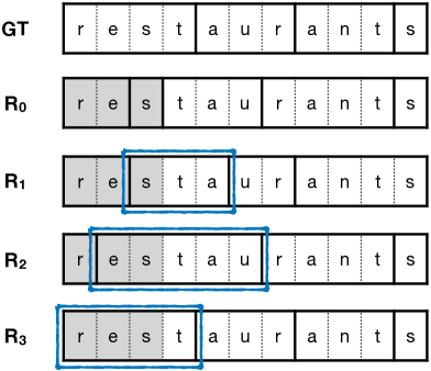
Figure 1: Illustration of retrace algorithm with the example of “restaurants.” The gray area means given prefix (“res”) of the query. The solid line indicates the boundary of the segmentation. GT is the segmentation of ground truth query. Possible examples of the generated sequence of tokens belonging to the case $R_{r}$ are visualized. Blue boxes indicate a fixed segmentation with retrace algorithm at the end of the prefix.

This process is unnecessary for a character-level model since every token is a single character. On the other hand, the retrace algorithm is helpful for subword models, especially BPE models which have deterministic segmentation algorithm.

We can limit the maximum step of retrace by $L$ to only consider $R_{r}$ where $0\leq r\leq L$ because of the computational issue. We will denote this limitation as $R^{L}$. $R^{0}$ is the usual case without the retrace algorithm, and $R^{\infty}$ counts every possible retrace steps.

4.2 Reranking Method by Approximate Marginalization

QAC system has to suggest $N$ completion candidates sorted in order of likelihood rather than finding only the best completion candidate. We can extract a set of top $B(\geq N)$ candidates using beam search with beam size $B$, namely $T_{B}=\{{\bf t}^{1},\cdots,{\bf t}^{B}\}$ in the descending order of likelihood. In the case of deterministic segmentation, ${\bf q}^{i}=concat({\bf t}^{i})$ are mutually different. i.e. $|Q_{B}|=B$ for $Q_{B}=\{{\bf q}^{1},\cdots,{\bf q}^{B}\}$. Then, trivially our prediction would be $({\bf q}^{1},\cdots,{\bf q}^{N})$.

On the other hand, in the case of stochastic segmentation, same query ${\bf q}^{i},{\bf q}^{j}(i\neq j)$ with different token sequence ${\bf t}^{i},{\bf t}^{j}$ may exist. The obvious way is merely removing duplicates.

On the assumption that $\log p({\bf t})\gg\log p({\bf t}^{\prime})$ for all ${\bf t}\in T_{B}$ and ${\bf t}^{\prime}\notin T_{B}$, Equation (1) implies that marginalization over the final beam outputs can provide better approximation:

$$\hat{{\bf q}} \approx\operatorname*{\arg\!\max}_{{\bf q}\in Q_{+}({\bf p})}\log\sum_{{\bf t}\in T_{B}}p({\bf t})$$

$$=\operatorname*{\arg\!\max}_{{\bf q}\in Q_{B}}\log\sum_{{\bf t}\in T_{B}}p({\bf t})$$

In other words, reranking after summing out the probability of duplicates can give better ordered list of candidates.

5 Evaluation Metric

5.1 MRR and PMRR

One of the most standard QAC evaluation metrics is the mean reciprocal rank (MRR). The MRR for the QAC system $m$ is calculated with test dataset $Q_{test}$ as follows:

$$MRR(m)=\frac{1}{|Q_{test}|}\sum_{{\bf q}\in Q_{test}}\mathrm{RR}({\bf q},m({\bf p})),$$

where ${\bf p}$ is a prefix of a query ${\bf q}$ and $m({\bf p})$ is the ranked list of candidate completions of ${\bf p}$ from $m$. $\mathrm{RR}$ is reciprocal rank of ${\bf q}$ if ${\bf q}$ is in $m({\bf p})$, otherwise 0.

Since it is hard to get a pair of the desired query and its prefix in a real situation, we should synthetically select a prefix by cutting off a given query for the evaluation. Common practice is to uniformly sample from all possible prefixes within minimal length constraint in characters (or words) However, real distribution of the prefix length may differ to the uniform distribution. For example, users tend to engage with QAC at the position close to the boundary of words, and after typing half of query characters Mitra et al. (2014). Due to the stochastic characteristic of prefix sampling processes or their difference among distinct QAC systems, evaluation results are inconsistent even with the same test dataset. To prevent this problem, a sampling function should be concretely specified.

Park and Chiba (2017) introduced a new metric, partial-matching MRR (PMRR):

$$PMRR(m)=\frac{1}{|Q_{test}|}\sum_{{\bf q}\in Q_{test}}\mathrm{PRR}({\bf q},m({\bf p})),$$

where partial-matching reciprocal rank $\mathrm{PRR}$ is the reciprocal of the index of the first candidate such that the original query is the same as it or starts with it plus whitespace. If there is no such candidate, $\mathrm{PRR}$ equals to 0.

PMRR also requires sampling of the prefix length. PMRR values are often omitted in the literature because of the similar tendency to MRR. In other words, PMRR does not give much additional information about the quality of the generated results.

5.2 Recoverable Length

To avoid the synthetic sampling process and length dependency, we propose a new evaluation metric for query auto-completion, namely mean recoverable length (MRL). We define recoverable length $\mathrm{RL}$ as the number of characters right before the first position where candidates do not have the query. When all characters of a query are known, we can readily suggest itself. If we delete chars from right to left one-by-one, the ground truth query will disappear in the list of candidate completions. For example, if ${\bf q}\in m({\bf q}_{1:|{\bf q}|-l})$ for $l=1,2,3$ but not $4$, recoverable length of this query with respect to the QAC system $m$ is 3. MRL is mean of recoverable length:

$$MRL(m)=\frac{1}{|Q_{test}|}\sum_{{\bf q}\in Q_{test}}\mathrm{RL}_{m}({\bf q})$$

MRL is a useful metric for additive QAC which suggests one word at a time instead of a whole-query completion Vargas et al. (2016) in that it measures how many characters the system can predict correctly at once. MRL does not care about the order of candidates and check whether they contain the target query or not. Lastly, it eliminates the need to choose a prefix length in the test data.

6 Experiments

Model	MRR			PMRR			MRL			Execution Speed (QPS)		Decode Length
	Seen	Unseen	All	Seen	Unseen	All	Seen	Unseen	All	CPU	GPU
MPC	.570	.000	.290	.616	.095	.360	8.06	0.00	4.10	$>$100		N/A
Char	.458	.160	.311	.552	.372	.464	5.77	4.24	5.02	11.0 (1.0x)	16.5 (1.0x)	14.5
BPE	.242	.085	.164	.305	.232	.269	0.49	0.54	0.51	24.2 (2.2x)	37.4 (2.3x)	7.1
BPE+R1	.427	.156	.294	.517	.368	.444	5.28	3.98	4.64	15.8 (1.4x)	27.3 (1.7x)	11.8
BPE+R2	.430	.157	.296	.520	.369	.446	5.44	4.01	4.74	15.5 (1.4x)	27.2 (1.6x)	12.2
BPE+R$\infty$	.431	.157	.296	.520	.369	.446	5.50	4.01	4.76	15.3 (1.4x)	26.9 (1.6x)	12.2
SR	.422	.148	.288	.541	.379	.461	5.11	3.82	4.48	20.8 (1.9x)	40.1 (2.4x)	6.8
SR+M	.424	.149	.289	.535	.373	.455	5.14	3.85	4.50	19.6 (1.8x)	40.0 (2.4x)	6.8
SR+R$\infty$	.423	.148	.289	.541	.378	.461	5.14	3.83	4.50	16.3 (1.5x)	29.6 (1.8x)	7.4
SR+R$\infty$+M	.427	.150	.291	.538	.375	.458	5.19	3.88	4.54	16.2 (1.5x)	28.7 (1.7x)	7.4

Table 1: Results of completion generation. We group MPC, character language model baseline, and two subword language models separately. +R implies the retrace algorithm. +M implies reranking with approximate marginalization. QPS stands for query per seconds. The higher the QPS, the better. The best results for each column related to accuracy are shown in bold for each segmentation algorithm (BPE and SR). SR model shows higher unseen PMRR scores (underlined). Our models are faster than the character baseline.

6.1 Data

We use the public AOL query log dataset Pass et al. (2006) for the experiments. We split data based on time. Among three months of the entire span, we use last one week as test data and one week right before the test data as validation data. It is close to a real scenario where future queries are unseen during the training.

We perform Unicode NFKC normalization and remove non-ASCII characters. For simplicity, we change uppercase alphabets to lowercase. After normalization and changing to lowercase, only 43 unique characters including special symbols BOS> , \verb EOS¿ and UNK¿ remain. We substituted multiple adjacent spaces to a single one and removed leading or trailing spaces. We merged duplicates which appear adjacently by the same user and the same query. Queries of a length shorter than three characters are filtered out. % for the test?

In total, the training, validation, test data contain 17,521,031, 1,521,971, and 1,317,632 queries, respectively. Among the test data, 670,810 queries are seen, and 646,822 queries are unseen in the training data. Almost half of the test data are unseen.

“subsection–Implementation Details˝ %“subsection–Model Architecture˝ “label–implementation˝ The language model used in the experiments consists of an input layer, a single LSTM layer, a projection layer, and an output layer. For the LSTM layer, following “citet–melis2017state˝ and “citet–jaech2018personalized˝, we apply layer normalization “cite–ba2016layer˝ to each gate and couple input and forget gates. We tie input and output embeddings for better generalization “cite–press2016using, inan2016tying˝. We set the LSTM hidden size to 600 and the input embedding size to 100.

We train three individual language models: namely Char, BPE, SR. The only difference among models is how to segment a given sentence into tokens. % tested combinations of input embedding size (25, 100) and hidden size (300: small, 600: large). %An LSTM layer takes a majority of overall model parameters. %% As the vocabulary size increases the required dimension size to represent each token increases. We believe that increasing model size (number of LSTM layers, input size, and hidden size) would improve the performance. Also, the best set of a combination may differ depending on models. However, we use the same model size for the character baseline and our variants for the fairness since our goal is proposing a new method and comparing between baseline and ours rather than achieving the best performance with the restriction of having a similar number of parameters. %%%%%%%%%% % We use various vocabulary sizes of “–256, 512, 1024“˝ for the subword segmentation. % Overall, we trained seven language models: namely Char, BPE“tsub–S˝, BPE“tsub–M˝, BPE“tsub–L˝, SR“tsub–S˝, SR“tsub–M˝, SR“tsub–L˝. % S, M, L corresponds to a vocabulary size of 256, 512, 1024, respectively.

We use the off-the-shelf SentencePiece “cite–kudo2018sentencepiece˝ library for vocabulary learning and segmentation of the vocabulary size 256 using BPE, SR algorithms. % unigram language model. For the subword regularization, we use sampling parameters $l=“infty$, $“alpha=0.2$ for the training. % dependence on SR parameters: we fix to l:inf, alpha:0.2 We choose this value by the generation accuracy on the validation data. Increase of model size and computation due to larger vocabulary size are not substantial. By setting a manageable amount of vocabulary size, we can balance performance and computational cost.

For the computational efficiency, we truncated queries in the training data to a length of 40. % characters. Only less than 3“% of queries in the training data are longer than 40 characters. We train models for thirty epochs by the Adam “cite–kingma2014adam˝ optimizer with a learning rate 5e-3 and batch size 1024. Following “citet–smith2018disciplined˝, we use a large learning rate and batch size. %It allows faster training until the final convergence. We use recurrent dropout “cite–semeniuta2016recurrent˝ with probability of 0.25 for regularization. The best model is chosen using validation data.

Using QAC models, we generate $N = 10$ completion candidates using beam search decoding of a beam width $B = 30$. %which is chosen based on the validation data. %For the beam search decoding to generate completions, 100 and a branching factor of 4.

For the SR models, the segmentation of $“pv$ (or retraced $“pv˙–1:—“pv—-r˝$) is not deterministic and generated completions may differ depending on its segmented token sequences with their different encoded representation. By following “cite–kudo2018subword˝, we can find the most likely segmentation sequence $“tv$ starting from all of the $n$-best segmentations $“tilde–“tv˝˙1, “cdots, “tilde–“tv˝˙n$ of $S(“pv)$ rather than from only $“tilde–“tv˝˙1$. However, we observe that this $n$-best decoding performs worse than one-best decoding. One possible reason is that segmentations which are not the best have a smaller probability as itself and so less likely to appear in training and less competitive in the process of beam search. For this reason, we set $n$ to 1. % For this reason, we did not report those values. % in Table ~“ref–tab:decode˝.

We used a trie “cite–fredkin1960trie˝ data structure to implement most popular completion baseline. % frequency based

All experiments were performed on NAVER Smart Machine Learning (NSML) platform “cite–sung2017nsml, kim2018nsml˝.

“subsection–Decoding Results˝ %“input–tab˙decode˝

%%% Explanation of variants We performed comprehensive experiments to analyze the performance of query auto-completion. Table~“ref–tab:decoding˝ shows the generation result of MPC, the character baseline, and our model variants. % We use the character baseline and variants of subword language models mentioned in Section “ref–implementation˝ for decoding. For BPE models, we varied the maximum retrace step to 0 (without retrace algorithm), 1, 2, and $“infty$ (no limitation on retracing step size). For SR models, we compare decoding results without any techniques, with marginalization only, with retrace algorithm only, and with both. % %We will add a table containing all of these results to the appendix. For the visibility, the representatives are chosen and put to Figure “ref–fig:decoding˝.

MPC is a very fast and remarkably strong baseline. It is worse than language models in the overall score (MRR, PMRR, and MRL), but better for previously seen queries. However, it is unable to predict unseen queries. Even with efficient data structures, MPC requires huge memory to keep statistics of all previous queries. As a practical view, combining frequency-based traditional method and neural language model approach can boost the accuracy and meet trade-off between the performance and computational costs.

%Trade off between MRR and PMRR? %%% MRR / PMRR % Models of small vocabulary size with retrace algorithms and marginalization performs best for both BPE and SR. MRRs and PMRRs of our best methods are close to that of the character model with less than 0.02 point drop. %%% Unseen PMRR -¿ better generalization %Subword models achieve much higher PMRR than the character baseline. -¿ No Notably, the SR model has better generalization ability in that their PMRR for unseen queries is higher than that of the character model. In a real scenario, it is more critical because unseen queries come in increasingly as time goes by. %%% $n$-best decoding

%%% Time: Execution speed, Decoding length % Execution speed is the number of queries processed every second (QPS). We measure execution time with Tesla P40 GPU and Xeon CPU. Subword-level models are up to 2.5 times faster than the character baseline with minimal loss in performance both in CPU and GPU. Decoding length which is maximum suffix length until beam search ends correlates with the number of floating-point operations. Subword models significantly reduce the decoding length from the character baseline more than two times shorter by generating multiple characters at once. %Decoding length of BPE is smaller than SR due to the deterministic nature of segmentation, resulting in much faster execution speed. -¿ No

%%% Retrace algorithm Models with additional techniques perform better than without them. Especially, retrace algorithm gives huge improvement for BPE case. Without retrace algorithm, BPE models do not work well. On the other hand, SR models only obtain small improvement. %BPE models with the retrace algorithm and all SR models achieve much higher PMRR than the character baseline. Because retrace algorithm goes back, it increases the decoding length and slows down the speed. % about 1-2 % a little Although current retrace algorithm is implemented straightforwardly, it can be improved by merging beams efficiently. Most of the subword lengths are equal or shorter than 3, so retrace of step 2 is quite enough, and R“tsup–2˝ get a close result with R“tsup–$“infty$˝. %By changing this limit, we observe -.

%%% Reranking by approximate marginalization The reranking method by approximate marginalization gives a small amount of improvement and is orthogonal to retrace algorithm. Marginalization method increases MRR but decreases PMRR. It is plausible in that it changes the order of candidates by reranking. The effect of marginalization would be better if we use a bigger beam size. Because the reranking process is done after beam search decoding which takes most of the decoding time and only consists of summation and sorting the final beam outputs, it does not take a long time.

%%% vocab size We also had experimented by increasing the vocabulary size. The accuracy of BPE models degrades fast as the vocabulary size increases. On the other hand, the performance of SR models is quite stable due to the regularization effect during training. As desired, the larger the dictionary size, the shorter the decoding length. %We can use a larger vocabulary size if faster decoding is needed. Whereas computations run in parallel in GPU, the number of operations for the output layer in the language model is proportional to the vocabulary size in CPU. Therefore, a larger vocabulary size does not always guarantee speedup for execution in the CPU. More thorough investigation about the correlation between QAC performance and the vocabulary size of subword language models remains for future work.

%“subsection–Qualitative Analysis˝ “input–tabs/example˝

“begin–figure*˝[t!] “centering “includegraphics[width=“textwidth]–figs/metric.pdf˝ “caption–Comparison of the character-level baseline model and our best models by changing query length and prefix length in terms of three evaluation metrics: MRR, PMRR, and MRL. MRL is only varied by query length because it does not require prefix length sampling.˝ “label–fig:metric˝ “end–figure*˝

Table “ref–tab:example˝ shows examples of decoding results. Our model generates more concise and realistic examples.

“subsection–Analysis on Evaluation Metrics˝

As shown in Figure~“ref–fig:metric˝, we compared our best models on three evaluation metrics (MRR, PMRR, and MRL) by changing the query length and prefix length. MRR and PMRR are more favorable to shorter queries. They drop very fast as the query becomes longer. % as seen in Figure %Same with MRR, PMRR tends to have a higher value for short queries. % of auto-regressive models usually tend to generate short completions. %even with length normalization “cite–wu2016google˝, For a longer query, the suffix length after sampling prefix has more chance to be longer. The search space increases exponentially with its suffix length. Even though QAC systems could generate realistic candidates, it is quite hard to match a long sequence with the ground truth. % Two methods of having similar MRR values might perform differently in reality. % In this sense, MRR is not good enough to evaluate the results of query auto-completion. As the prefix length becomes longer which means that much information for determining the query has been given, the completion performance improves.

Interestingly, MRR and MRL of BPE are higher than those of SR, although BPE is worse in terms of PMRR than SR. For short queries, SR outperforms the character baseline. On the other hand, BPE is poor when the query length (or prefix length) is short. However, for a longer case, its MRR is almost close to that of the character baseline.

%%% MRL %Our best methods also achieve similar MRL with the character baseline (5.02): 4.76 and 4.54 for BPE and SR, respectively, with the retrace algorithm and reranking method. MRR and PMRR are highly dependent on the length distribution of test data. % Moreover, as shown in Table “ref–tab:decode˝, MRL is more fine-grained. In contrast, MRL keeps the order between different methods as the query length changes. %, but other metrics do not. MRL is more reliable in the respect that it could provide consistent order between methods regardless of query length distribution. % we have observed that MRL is more fine-grained than MRR and PMRR. % Length dependency %On the other hand, PMRR and MRL are less dependent on the query’s length. For long queries lengths, MRL stays in the flat area. Normalizing recoverable length based on the query length might be necessary. %and is an open problem.

7 Future Work

Approximation in training (Section 3.2) and decoding (Section 4) deteriorate the accuracy of subword language modeling. One possible solution to reduce the accuracy gap between the character language model baseline and the subword language model is knowledge distillation Hinton et al. (2015); Kim and Rush (2016); Liu et al. (2018) from character-level language models. A student model can learn to match an estimation of query probability with that of a teacher model.

Another interesting research direction is learning segmentation jointly with language model Kawakami et al. (2019); Grave et al. (2019) rather than using fixed pretrained segmentation algorithms. A conditional semi-Markov assumption allows exact marginalization using dynamic programming Ling et al. (2016); Wang et al. (2017). Nevertheless, beam search decoding on those language models, especially faster decoding, is non-trivial.

Proposed method can be extended to wide range of tasks. Query suggestion Sordoni et al. (2015); Dehghani et al. (2017) and query reformulation Nogueira and Cho (2017) are related to QAC and well-established problems. They both are also possible applications of the subword-level modeling. Drexler and Glass (2019) used subword regularization and beam search decoding for end-to-end automatic speech recognition.

Lastly, implementation with more advanced data structure Hsu and Ottaviano (2013) and parallel algorithms to speed up and meet memory limitation are necessary for the real deployment Wang et al. (2018). It would be helpful if the computation is adaptively controllable on-the-fly Graves (2016) at the runtime depending on the situation.

8 Conclusion

In this paper, we propose subword language models for query auto-completion with additional techniques, retrace algorithm and reranking with approximate marginalization. We observed subword language models significant speedup compared to the character-level baseline while maintaining the generation quality. Our best models achieve up to 2.5 times faster decoding speed with less than 0.02 point drop of MRR and PMRR.

Using a subword language model, we build an accurate and much faster QAC system compared to the character-level language model baseline. Although there is still much room for improvement on hyperparameter optimization, decoding search, and neural architectures like Transformer Vaswani et al. (2017); Dai et al. (2019), the goal of this work is to prove that the subword language model is an attractive choice for QAC as an alternative to the character-level language model, especially if latency is considered.

We believe that our newly proposed metric, mean recoverable length (MRL), provides fruitful information for the QAC research in addition to conventional evaluation metric based on ranks.

References

- Al-Rfou et al. (2018) Rami Al-Rfou, Dokook Choe, Noah Constant, Mandy Guo, and Llion Jones. 2018. Character-level language modeling with deeper self-attention. arXiv preprint arXiv:1808.04444.
- Ba et al. (2016) Jimmy Lei Ba, Jamie Ryan Kiros, and Geoffrey E Hinton. 2016. Layer normalization. arXiv preprint arXiv:1607.06450.
- Bar-Yossef and Kraus (2011) Ziv Bar-Yossef and Naama Kraus. 2011. Context-sensitive query auto-completion. In Proceedings of the 20th international conference on World wide web, pages 107–116. ACM.
- Burges (2010) Christopher JC Burges. 2010. From ranknet to lambdarank to lambdamart: An overview. Learning, 11(23-581):81.
- Cai et al. (2016) Fei Cai, Maarten De Rijke, et al. 2016. A survey of query auto completion in information retrieval. Foundations and Trends® in Information Retrieval, 10(4):273–363.
- Chan et al. (2016) William Chan, Yu Zhang, Quoc Le, and Navdeep Jaitly. 2016. Latent sequence decompositions. arXiv preprint arXiv:1610.03035.
- Chung et al. (2016) Junyoung Chung, Kyunghyun Cho, and Yoshua Bengio. 2016. A character-level decoder without explicit segmentation for neural machine translation. arXiv preprint arXiv:1603.06147.
- Conneau et al. (2016) Alexis Conneau, Holger Schwenk, Loïc Barrault, and Yann Lecun. 2016. Very deep convolutional networks for text classification. arXiv preprint arXiv:1606.01781.
- Dai et al. (2019) Zihang Dai, Zhilin Yang, Yiming Yang, William W Cohen, Jaime Carbonell, Quoc V Le, and Ruslan Salakhutdinov. 2019. Transformer-xl: Attentive language models beyond a fixed-length context. arXiv preprint arXiv:1901.02860.
- Dehghani et al. (2017) Mostafa Dehghani, Sascha Rothe, Enrique Alfonseca, and Pascal Fleury. 2017. Learning to attend, copy, and generate for session-based query suggestion. In Proceedings of the 2017 ACM on Conference on Information and Knowledge Management, pages 1747–1756. ACM.
- Devlin et al. (2018) Jacob Devlin, Ming-Wei Chang, Kenton Lee, and Kristina Toutanova. 2018. Bert: Pre-training of deep bidirectional transformers for language understanding. arXiv preprint arXiv:1810.04805.
- Drexler and Glass (2019) Jennifer Drexler and James Glass. 2019. Subword regularization and beam search decoding for end-to-end automatic speech recognition. In ICASSP 2019-2019 IEEE International Conference on Acoustics, Speech and Signal Processing (ICASSP), pages 6266–6270. IEEE.
- Fiorini and Lu (2018) Nicolas Fiorini and Zhiyong Lu. 2018. Personalized neural language models for real-world query auto completion. arXiv preprint arXiv:1804.06439.
- Fredkin (1960) Edward Fredkin. 1960. Trie memory. Communications of the ACM, 3(9):490–499.
- Grave et al. (2019) Édouard Grave, Sainbayar Sukhbaatar, Piotr Bojanowski, and Armand Joulin. 2019. Training hybrid language models by marginalizing over segmentations. In Proceedings of the 57th Conference of the Association for Computational Linguistics, pages 1477–1482.
- Graves (2016) Alex Graves. 2016. Adaptive computation time for recurrent neural networks. arXiv preprint arXiv:1603.08983.
- Gu et al. (2017) Jiatao Gu, James Bradbury, Caiming Xiong, Victor OK Li, and Richard Socher. 2017. Non-autoregressive neural machine translation. arXiv preprint arXiv:1711.02281.
- Hinton et al. (2015) Geoffrey Hinton, Oriol Vinyals, and Jeff Dean. 2015. Distilling the knowledge in a neural network. arXiv preprint arXiv:1503.02531.
- Hsu and Ottaviano (2013) Bo-June Paul Hsu and Giuseppe Ottaviano. 2013. Space-efficient data structures for top-k completion. In Proceedings of the 22nd international conference on World Wide Web, pages 583–594. ACM.
- Hwang and Sung (2017) Kyuyeon Hwang and Wonyong Sung. 2017. Character-level language modeling with hierarchical recurrent neural networks. In Acoustics, Speech and Signal Processing (ICASSP), 2017 IEEE International Conference on, pages 5720–5724. IEEE.
- Inan et al. (2016) Hakan Inan, Khashayar Khosravi, and Richard Socher. 2016. Tying word vectors and word classifiers: A loss framework for language modeling. arXiv preprint arXiv:1611.01462.
- Jaech and Ostendorf (2018) Aaron Jaech and Mari Ostendorf. 2018. Personalized language model for query auto-completion. arXiv preprint arXiv:1804.09661.
- Kawakami et al. (2019) Kazuya Kawakami, Chris Dyer, and Phil Blunsom. 2019. Learning to discover, ground and use words with segmental neural language models. In Proceedings of the 57th Conference of the Association for Computational Linguistics, pages 6429–6441.
- Kim et al. (2018) Hanjoo Kim, Minkyu Kim, Dongjoo Seo, Jinwoong Kim, Heungseok Park, Soeun Park, Hyunwoo Jo, KyungHyun Kim, Youngil Yang, Youngkwan Kim, et al. 2018. Nsml: Meet the mlaas platform with a real-world case study. arXiv preprint arXiv:1810.09957.
- Kim (2014) Yoon Kim. 2014. Convolutional neural networks for sentence classification. arXiv preprint arXiv:1408.5882.
- Kim et al. (2016) Yoon Kim, Yacine Jernite, David Sontag, and Alexander M Rush. 2016. Character-aware neural language models. In AAAI, pages 2741–2749.
- Kim and Rush (2016) Yoon Kim and Alexander M Rush. 2016. Sequence-level knowledge distillation. arXiv preprint arXiv:1606.07947.
- Kingma and Ba (2014) Diederik P Kingma and Jimmy Ba. 2014. Adam: A method for stochastic optimization. arXiv preprint arXiv:1412.6980.
- Kudo (2018) Taku Kudo. 2018. Subword regularization: Improving neural network translation models with multiple subword candidates. ACL.
- Kudo and Richardson (2018) Taku Kudo and John Richardson. 2018. Sentencepiece: A simple and language independent subword tokenizer and detokenizer for neural text processing. arXiv preprint arXiv:1808.06226.
- Lee et al. (2017) Jason Lee, Kyunghyun Cho, and Thomas Hofmann. 2017. Fully character-level neural machine translation without explicit segmentation. Transactions of the Association for Computational Linguistics, 5:365–378.
- Lee et al. (2018) Jason Lee, Elman Mansimov, and Kyunghyun Cho. 2018. Deterministic non-autoregressive neural sequence modeling by iterative refinement. arXiv preprint arXiv:1802.06901.
- Ling et al. (2016) Wang Ling, Edward Grefenstette, Karl Moritz Hermann, Tomáš Kočiskỳ, Andrew Senior, Fumin Wang, and Phil Blunsom. 2016. Latent predictor networks for code generation. arXiv preprint arXiv:1603.06744.
- Liu et al. (2018) Yijia Liu, Wanxiang Che, Huaipeng Zhao, Bing Qin, and Ting Liu. 2018. Distilling knowledge for search-based structured prediction. arXiv preprint arXiv:1805.11224.
- Luong and Manning (2016) Minh-Thang Luong and Christopher D Manning. 2016. Achieving open vocabulary neural machine translation with hybrid word-character models. arXiv preprint arXiv:1604.00788.
- Melis et al. (2017) Gábor Melis, Chris Dyer, and Phil Blunsom. 2017. On the state of the art of evaluation in neural language models. arXiv preprint arXiv:1707.05589.
- Mikolov et al. (2012) Tomáš Mikolov, Ilya Sutskever, Anoop Deoras, Hai-Son Le, Stefan Kombrink, and Jan Cernocky. 2012. Subword language modeling with neural networks. preprint (http://www. fit. vutbr. cz/imikolov/rnnlm/char. pdf), 8.
- Mitra et al. (2014) Bhaskar Mitra, Milad Shokouhi, Filip Radlinski, and Katja Hofmann. 2014. On user interactions with query auto-completion. In Proceedings of the 37th international ACM SIGIR conference on Research & development in information retrieval, pages 1055–1058. ACM.
- Miyamoto and Cho (2016) Yasumasa Miyamoto and Kyunghyun Cho. 2016. Gated word-character recurrent language model. arXiv preprint arXiv:1606.01700.
- Nogueira and Cho (2017) Rodrigo Nogueira and Kyunghyun Cho. 2017. Task-oriented query reformulation with reinforcement learning. arXiv preprint arXiv:1704.04572.
- Park and Chiba (2017) Dae Hoon Park and Rikio Chiba. 2017. A neural language model for query auto-completion. In Proceedings of the 40th International ACM SIGIR Conference on Research and Development in Information Retrieval, pages 1189–1192. ACM.
- Pass et al. (2006) Greg Pass, Abdur Chowdhury, and Cayley Torgeson. 2006. A picture of search. In InfoScale, volume 152, page 1.
- Press and Wolf (2016) Ofir Press and Lior Wolf. 2016. Using the output embedding to improve language models. arXiv preprint arXiv:1608.05859.
- Rumelhart et al. (1986) David E Rumelhart, Geoffrey E Hinton, and Ronald J Williams. 1986. Learning representations by back-propagating errors. nature, 323(6088):533.
- Semeniuta et al. (2016) Stanislau Semeniuta, Aliaksei Severyn, and Erhardt Barth. 2016. Recurrent dropout without memory loss. arXiv preprint arXiv:1603.05118.
- Sennrich (2016) Rico Sennrich. 2016. How grammatical is character-level neural machine translation? assessing mt quality with contrastive translation pairs. arXiv preprint arXiv:1612.04629.
- Sennrich et al. (2015) Rico Sennrich, Barry Haddow, and Alexandra Birch. 2015. Neural machine translation of rare words with subword units. arXiv preprint arXiv:1508.07909.
- Smith (2018) Leslie N Smith. 2018. A disciplined approach to neural network hyper-parameters: Part 1–learning rate, batch size, momentum, and weight decay. arXiv preprint arXiv:1803.09820.
- Sordoni et al. (2015) Alessandro Sordoni, Yoshua Bengio, Hossein Vahabi, Christina Lioma, Jakob Grue Simonsen, and Jian-Yun Nie. 2015. A hierarchical recurrent encoder-decoder for generative context-aware query suggestion. In Proceedings of the 24th ACM International on Conference on Information and Knowledge Management, pages 553–562. ACM.
- Stern et al. (2018) Mitchell Stern, Noam Shazeer, and Jakob Uszkoreit. 2018. Blockwise parallel decoding for deep autoregressive models. In Advances in Neural Information Processing Systems, pages 10106–10115.
- Sung et al. (2017) Nako Sung, Minkyu Kim, Hyunwoo Jo, Youngil Yang, Jingwoong Kim, Leonard Lausen, Youngkwan Kim, Gayoung Lee, Donghyun Kwak, Jung-Woo Ha, et al. 2017. Nsml: A machine learning platform that enables you to focus on your models. arXiv preprint arXiv:1712.05902.
- Vargas et al. (2016) Saúl Vargas, Roi Blanco, and Peter Mika. 2016. Term-by-term query auto-completion for mobile search. In Proceedings of the Ninth ACM International Conference on Web Search and Data Mining, pages 143–152. ACM.
- Vaswani et al. (2017) Ashish Vaswani, Noam Shazeer, Niki Parmar, Jakob Uszkoreit, Llion Jones, Aidan N Gomez, Łukasz Kaiser, and Illia Polosukhin. 2017. Attention is all you need. In Advances in neural information processing systems, pages 5998–6008.
- Wang et al. (2017) Chong Wang, Yining Wang, Po-Sen Huang, Abdelrahman Mohamed, Dengyong Zhou, and Li Deng. 2017. Sequence modeling via segmentations. In Proceedings of the 34th International Conference on Machine Learning-Volume 70, pages 3674–3683. JMLR. org.
- Wang et al. (2018) Po-Wei Wang, J Zico Kolter, Vijai Mohan, and Inderjit S Dhillon. 2018. Realtime query completion via deep language models. SIGIR eCom.
- Williams (1992) Ronald J Williams. 1992. Simple statistical gradient-following algorithms for connectionist reinforcement learning. Machine learning, 8(3-4):229–256.
- Wu et al. (2016) Yonghui Wu, Mike Schuster, Zhifeng Chen, Quoc V Le, Mohammad Norouzi, Wolfgang Macherey, Maxim Krikun, Yuan Cao, Qin Gao, Klaus Macherey, et al. 2016. Google’s neural machine translation system: Bridging the gap between human and machine translation. arXiv preprint arXiv:1609.08144.
- Zhang et al. (2015) Xiang Zhang, Junbo Zhao, and Yann LeCun. 2015. Character-level convolutional networks for text classification. In Advances in neural information processing systems, pages 649–657.