Abstract

Our main aim in this paper is to constrain the effective field theory describing the top quark couplings through the $e^{-}e^{+}\rightarrow t\bar{t}+$jet process. The analysis is carried out considering two different center-of-mass energies of 500 and 3000 GeV including a realistic simulation of the detector response and the main sources of background processes. The expected limits at 95% CL are derived on the new physics couplings such as $t\bar{t}\gamma$, $t\bar{t}Z$, and $t\bar{t}g$ for each benchmark scenario using the dileptonic $t\bar{t}$ final state. We show that the 95% CL limits on dimensionless Wilson coefficients $\bar{c}_{i}$ considered in this analysis could be probed down to $10^{-4}$.

1 Introduction

Since the Higgs boson observation [1, 2] at the Large Hadron Collider (LHC) by the ATLAS and CMS Collaborations, the primary focus of high energy particle physics is to probe its properties in details [3, 4, 5]. In addition to the Higgs boson, the heaviest discovered particle to date, i.e. the top quark which was discovered by D0 and CDF Collaborations at Fermilab [6, 7], is expected to play an important role in the electroweak symmetry breaking (EWSB) mechanism due to its large mass.

Looking further into the future, in addition to the LHC, precision measurements of the top quark and Higgs boson properties motivate the construction of future lepton colliders which provide cleaner environments due to the absence of hadronic initial state and their relatively smaller experimental uncertainties with respect to the hadron colliders. Hence, there is currently a growing interest in studying physics accessible by possible future high-energy and high-luminosity electron-positron colliders that would continue the investigations made with the large electron-positron (LEP) collider to much higher energy and luminosity [8, 9, 10]. So far, there have been several proposals over the past years for the future electron-positron colliders, such as the Compact Linear Collider (CLIC) [11, 12, 13], the International Linear Collider (ILC) [14, 15, 16], Circular Electron Positron Collider (CPEC) [17, 18], and the highest-luminosity energy frontier Future Circular Collider with electron-positron collisions (FCC-ee) at CERN [19], previously known as TLEP [20] (see, for example, the most recent Conceptual Design Report by FCC Collaboration [21, 22] for recent review.).

Phenomenological and experimental studies over the past decades have provided important information on the validity of the Standard Model (SM) as well as the physics beyond the SM (BSM) [23, 24, 25]. The focus of many studies has been on the top quark and Higgs boson phenomenology and search for the new physics through them. These include, for example, the precise measurements of the top quark and Higgs boson masses, their couplings to the other fundamental particles in the framework of the SM and BSM, and searches for new physics effects beyond the SM in both model dependent and independent ways. In the case that the possible new degrees of freedom are not light enough to be directly produced at a collider, they could affect the SM observables indirectly through virtual effects. In such conditions, a powerful tool to parametrise any potential deviations from the SM predictions in a model-independent way is the standard model effective field theory (SMEFT). SMEFT provides a general framework where non-redundant bases of independent operators can be built and one would be able to match them to explicit ultraviolet complete (UV-complete) models in a systematic way. From the phenomenological point of view, there is a large volume of published works to study the SMEFT in particular in the top quark and Higgs boson sectors from the LHC, from electron-positron colliders, and from future proposed high-energy lepton-hadron and hadron-hadron colliders [26, 27, 28, 29, 30, 31, 32, 33, 34, 35, 36, 37, 38, 39, 40, 41, 42, 43, 44, 45, 46, 47, 48, 49, 50, 51, 52, 53, 54, 55, 63, 64, 56, 65, 57, 58, 59, 60, 61, 62, 66].

The aim of the present study is to examine the sensitivity of the top quark pair production in association with a jet at future electron-positron colliders to the SMEFT. All dimension-six operators in the SILH basis which involve top quark and/or Higgs and gauge bosons assuming CP-conservation are included [67, 68]. It is notable that flavour universality is assumed in the SILH basis.

We perform detailed sensitivity studies and present the expected 95% CL limits on the operator coefficients for the center-of-mass energies of 500 and 3000 GeV with integrated luminosities $\cal L$ related to the proposed electron-positron colliders. It is shown that including the $e^{-}e^{+}\rightarrow t\bar{t}+$jet process to $e^{-}e^{+}\rightarrow t\bar{t}$, improves the sensitivity to the effective couplings of top quark with the electroweak gauge bosons.

This paper is organised as follows: In section 2, the SMEFT framework is briefly introduced. In section 3, the details of the simulation for probing SMEFT operators through the production processes of $t\bar{t}$ in association with a jet at the electron-positron collision are described. In section 4, the methodology applied in this analysis to constrain the Wilson coefficients, as well as the results, are presented. Finally, section 5 concludes the paper.

2 Theoretical framework

As no clear evidence of new physics beyond the standard model has been observed, an efficient approach for examining the SM and possible deviations from SM could be provided by the SMEFT. In this approach, beyond the SM effects are probed via a series of higher dimensional SM operators. The coefficients of the operators, so-called Wilson coefficients, can be connected to the parameters of explicit models. The effective Lagrangian is provided considering the operators which are invariant under the ${\rm SU}(3)\times{\rm SU}(2)\times{\rm U}(1)$ gauge symmetries and Lorentz transformations. We restrict ourselves to the operators with a lepton and baryon number conservation. In such a case, the leading contributions come from dimension-six operators. The general Lagrangian of the SM effective theory with dimension-six operators is given by [69, 70, 71],

$${\cal L}_{\rm SMEFT}={\cal L}_{\rm SM}+\sum_{i}\frac{c_{i}{\cal O}_{i}}{\Lambda^{2}},$$ (1)

In the above relation, $\Lambda$ is the energy scale of new physics, $c_{i}$’s are dimensionless Wilson coefficients and the gauge-invariant dimension-six operators denoted by ${\cal O}_{i}$ are constructed out of the SM fields. There are various bases where the operators ${\cal O}_{i}$ are classified in an independent way. In this work, the dimension-six operators sensitive to the $e^{-}e^{+}\rightarrow t\bar{t}+$jet process are discussed in the SILH basis [72, 73, 74, 67]. This basis is not a unique basis and can be connected to the other bases. The SMEFT Lagrangian $\cal L_{\rm SMEFT}$ in the SILH basis can be expressed as follows:

$${\cal L}_{\rm SMEFT}={\cal L}_{\rm SM}+{\cal L}_{\rm SILH}+{\cal L}_{F_{1}}+{\cal L}_{F_{2}}+{\cal L}_{\rm G}+{\cal L}_{\rm CP}\,.$$ (2)

The first term in the above effective Lagrangian, ${\cal L}_{\rm SM}$, is the well-known SM Lagrangian. The second term, ${\cal L}_{\rm SILH}$, consists of a set of operators which involve the Higgs doublet $\Phi$ and could arise from UV-models where Higgs boson contributes to the strongly interacting sector. The interactions between two Higgs boson fields and a pair of quarks or a pair of leptons are described by ${\cal L}_{F_{1}}$ while the interactions of a quark pair or a lepton pair with one single Higgs field and a gauge boson are addressed by ${\cal L}_{F_{2}}$. All the modifications related to the gauge sector, from the gauge bosons self energies to the gauge bosons self-interactions are parameterized in ${\cal L}_{\rm G}$. The CP-violating interactions are described by ${\cal L}_{\rm CP}$. In this work, the concentration is on the CP-conserving operators.

Within the SMEFT framework, in addition to the new Feynman diagrams contributing to the $e^{-}e^{+}\rightarrow t\bar{t}+$jet, the SM Feynman diagrams are modified. The representative Feynman diagrams for the top quark pair and $t\bar{t}(+$jet) production at electron-positron colliders are depicted in Fig. 1. The filled circles are the vertices that receive modification from the SM effective field theory. It is notable that in addition to the diagrams for the $t\bar{t}g$ production where the SM couplings are modified, a new diagram arising from $hgt\bar{t}$ contribute to the $e^{-}e^{+}\rightarrow t\bar{t}+$jet process. The contribution of this diagram is small due to the presence of a Higgs boson Yukawa coupling with electron.

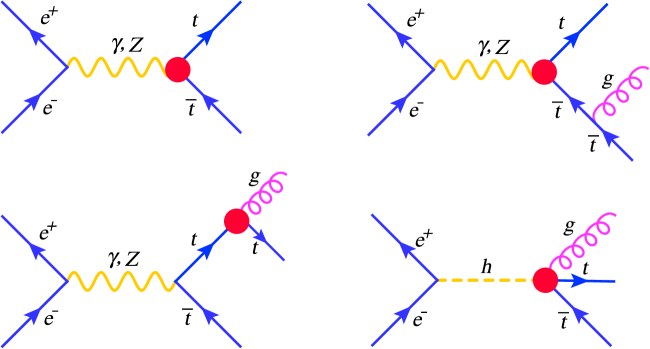
Figure 1: Representative Feynman diagrams for the $t\bar{t}$ and $t\bar{t}$ production in association with a jet in electron-positron collisions in the SMEFT.

In the current study, we restrict ourselves to effective operators contributing to $e^{-}e^{+}\rightarrow t\bar{t}+\text{jet}$ process involving at least one top quark. Although other effective operators can affect the $t\bar{t}+\text{jet}$ process via for example $Zee$ or $\gamma ee$ vertices, they have tightly constrained by the LEP and electroweak precision observables (EWPO). The CP-conserving operators in the SILH basis that affect the top quark interactions at leading order in the $t\bar{t}+\text{jet}$ are listed below:

$$\mathcal{O}_{uW} = {\bar{Q}}_{L}\sigma^{i}H^{c}\sigma^{\mu\nu}u_{R}\,W_{\mu\nu}^{i},$$

$$\mathcal{O}_{uB} = {\bar{Q}}_{L}H^{c}\sigma^{\mu\nu}u_{R}\,B_{\mu\nu},$$

$$\mathcal{O}_{uG} = {\bar{Q}}_{L}H^{c}\sigma^{\mu\nu}\lambda^{a}u_{R}\,G_{\mu\nu}^{a},\,$$

$$\mathcal{O}_{HQ} = \left(\bar{Q}_{L}\gamma^{\mu}Q_{L}\right)\big{(}H^{\dagger}{\overleftrightarrow{D}}_{\mu}H\big{)}$$

$$\mathcal{O}^{\prime}_{HQ} = \left(\bar{Q}_{L}\gamma^{\mu}\sigma^{i}Q_{L}\right)\big{(}H^{\dagger}\sigma^{i}{\overleftrightarrow{D}}_{\mu}H\big{)},$$

$$\mathcal{O}_{Hu} = \left(\bar{u}_{R}\gamma^{\mu}u_{R}\right)\big{(}H^{\dagger}{\overleftrightarrow{D}}_{\mu}H\big{)},$$ (3)

where the left-handed and right-handed quarks are denoted by $Q_{L}$ and $u_{R}$, respectively and $H^{\dagger}{\overleftrightarrow{D}}_{\mu}H\equiv H^{\dagger}D_{\mu}H-D_{\mu}H^{\dagger}H$.

Among the mentioned operators, $\mathcal{O}_{uG}$ modifies the interaction of the top quark and gluons, i.e. $gt\bar{t}$ and generates the new four-leg interaction of $hgt\bar{t}$ which contributes to the $t\bar{t}g$ production. The $\mathcal{O}_{uW}$, $\mathcal{O}_{uB}$, $\mathcal{O}_{HQ}$, $\mathcal{O}^{\prime}_{HQ}$, and $\mathcal{O}_{Hu}$ operators modify the interactions between the top quark, photon and the $Z$ boson.

The $\mathcal{O}_{uW}$ and $\mathcal{O}_{uB}$ operators modify the oblique parameters $S,T,$ and $U$ at one loop level. In particular, the $\bar{c}_{uW}$ and $\bar{c}_{uB}$ Wilson coefficients have been constrained at percent level using the oblique parameters [75]. Recent measurements of the $t\bar{t}Z$ and $t\bar{t}W$ processes by the CMS collaboration have provided the following bounds on $\bar{c}_{uG}$, $\bar{c}_{uW}$, $\bar{c}_{uB}$, and $\bar{c}_{Hu}$ [76, 77]:

$$-0.14\leq\bar{c}_{uW}\leq 0.14~{},~{}0.0\leq\bar{c}_{uB}\leq 0.13~{},~{}-0.07\leq\bar{c}_{uG}\leq 0.2~{},~{}-0.64\leq\bar{c}_{Hu}\leq 0.12,$$ (4)

Based on the global fit of the experimental data from the Tevatron, and LHC Runs I and II to the SM effective field theory, more stringent bounds on these Wilson coefficients could be derived [46, 78, 79, 80]. The derived constraints on the considered Wilson coefficients in this work from a global fit to the top quark experimental data are [46]:

$$-8.2\times 10^{-4}\leq\bar{c}_{uG}\leq 1.8\times 10^{-3},-4.6\times 10^{-2}\leq\bar{c}_{uB}\leq 7.0\times 10^{-2},-0.593\leq\bar{c}_{Hu}\leq 0.496,$$

$$-8.9\times 10^{-3}\leq\bar{c}_{uW}\leq 6.5\times 10^{-3},-0.369\leq\bar{c}_{HQ}\leq 0.375,-3.92\times 10^{-2}\leq\bar{c^{\prime}}_{HQ}\leq 2.27\times 10^{-2},$$ (5)

The imaginary parts of some of the coefficients of these operators can be constrained using the upper limit on the neutron electric dipole moment. The derived upper bound on Im($\bar{c}_{uG}$) at $95\%$ CL is of the order of $10^{-4}$ [74].

In order to calculate the impacts of the operators on the top quark pair production in association with a jet, MadGraph5_aMC@NLO [81, 82, 83] package is used. The effective SM Lagrangian introduced in Eq. (2) is implemented in the FeynRule program [84] and then the Universal FeynRules Output (UFO) model [85] is fed to the MadGraph5_aMC@NLO program. Top quark pair is produced with up to one additional parton in the final state using leading-order matrix elements. The 0-, 1-parton events are merged using the MLM matching scheme [86].

Figure 2 shows the $t\bar{t}+$(jet) production cross section as a function of the centre-of-mass energy at leading order for three signal scenarios as well as the SM background. In this figure the Wilson coefficients are normalised to the bar notation, $\bar{c}_{X}=c_{X}v^{2}/\Lambda^{2}$, and the $\mathcal{O}_{uG}$, $\mathcal{O}_{uW}$, and $\mathcal{O}_{uB}$ operators are individually switched on. As it can be seen, there is a significant enhancement which occurs at top quark pair threshold. For the SM, the production rate approximately falls down as $1/\sqrt{s}$. At $\sqrt{s}=3$ TeV, the cross section due to the presence of operator $\mathcal{O}_{uG}$ with $\bar{c}_{uG}=0.03$ increase by a factor of around two with respect to the SM while the enhancements arising from $\mathcal{O}_{uW}$ and $\mathcal{O}_{uB}$ with $\bar{c}_{uW}=0.03$ and $\bar{c}_{uB}=0.03$ are at the order of $20$ and $40$, respectively. Such raises of the cross section occur because of the momentum dependence of the $\mathcal{O}_{uW}$, $\mathcal{O}_{uB}$, and $\mathcal{O}_{uG}$ operators. The $\mathcal{O}_{uW}$ and $\mathcal{O}_{uB}$ operators lead to much larger increase in the cross section of signal with respect to $\mathcal{O}_{uG}$ because the involved virtual photon and $Z$ boson momenta could grow up to the total electron-positron center-of-mass energy while less momentum is running to the $\mathcal{O}_{uG}$ vertex. As mentioned previously, in this analysis the main aim is to examine the potential of the future lepton colliders to probe the SMEFT via the top quark pair production in association with a jet. In this work, in addition to $\bar{c}_{uB}$, $\bar{c}_{uG}$ and $\bar{c}_{uW}$, we examine $\bar{c}_{Hu}$, $\bar{c}_{HQ}$, and $\bar{c}^{\prime}_{HQ}$ .

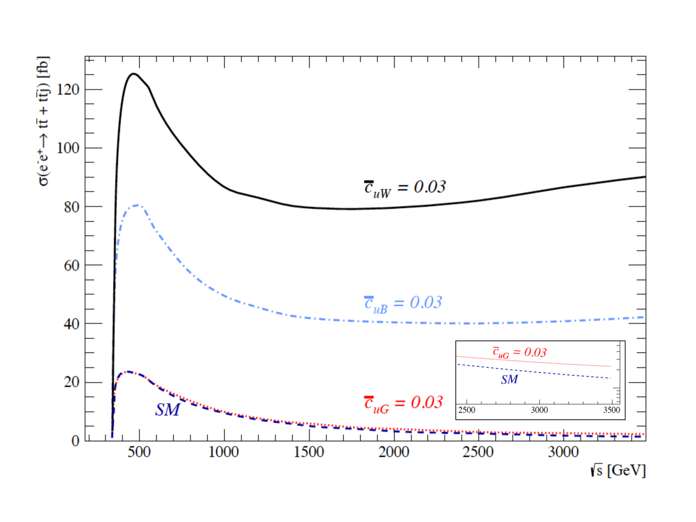
Figure 2: The leading order cross section for the production of $e^{-}e^{+}\rightarrow t\bar{t}+t\bar{t}j$ (merged using MLM) versus the center-of-mass energy. The results are shown for the SM and for the signal scenarios in bar notation $\bar{c}_{X}=c_{X}v^{2}/\Lambda^{2}$ with the assumptions of $\bar{c}_{uG}=0.03$, $\bar{c}_{uW}=0.03$, and $\bar{c}_{uB}=0.03$. The cross sections have been calculated with a minimum cut of $p_{\rm T}\geq 20$ GeV on the gluon. The small plot in the bottom shows the cross section for the SM and for $\bar{c}_{uG}=0.03$ in log-scale.

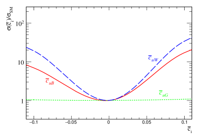
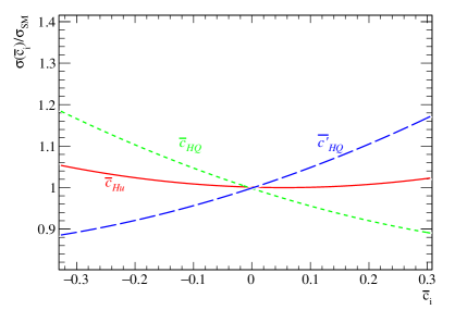
Figure 3: Ratio of $t\bar{t}+$jet production cross section in the SMEFT to the SM in electron-positron collisions versus the Wilson coefficients. The rates are calculated at leading-order at $\sqrt{s}=500$ GeV for the $\bar{c}_{uG}$, $\bar{c}_{uW}$, $\bar{c}_{uB}$, $\bar{c}_{HQ}$, $\bar{c}^{\prime}_{HQ}$, and $\bar{c}_{Hu}$. A minimum cut of 20 GeV has been applied on the transverse momentum of additional jet.

Figure 3 shows the ratio of the production cross section of signal process in the SMEFT to the SM in terms of the Wilson coefficients $\bar{c}_{uG}$, $\bar{c}_{uW}$, $\bar{c}_{uB}$, $\bar{c}_{HQ}$, $\bar{c}^{\prime}_{HQ}$, and $\bar{c}_{Hu}$. To calculate the cross sections, a minimum cut of 20 GeV has been applied on the gluon $p_{T}$. As it can be seen in the left plot of Fig.3, there is a remarkable sensitivity to $\bar{c}_{uW}$ and $\bar{c}_{uB}$ while $\bar{c}_{uG}$ has less impact on the production cross section. From the right plot in Fig. 3, we observe that $\bar{c}_{HQ}$, $\bar{c}^{\prime}_{HQ}$, and $\bar{c}_{Hu}$ have no considerable effect in the cross section with respect to $\bar{c}_{uW}$, $\bar{c}_{uB}$, and $\bar{c}_{uG}$. In the analysis we probe these Wilson coefficients at two different center-of-mass energies of 500 and 3000 GeV.

3 Simulation and details of the analysis

In this section, the details of the simulation and the analysis strategy to examine the dimension-six operators mentioned in Eq.2 using the top quark pair production in association with a jet are discussed. Based on the decay of $t\bar{t}$ system, there are three different final states for the signal: fully hadronic, semileptonic, and dileptonic final states with the branching fractions of $46.2\%$, $43.5\%$, and $10.3\%$, respectively. In this work, in order to have a clean signature, we focus on the dileptonic decay channel therefore the final state consists of at least two jets from which two are $b$-jets originating from the top quarks decay, two opposite sign charged leptons, and missing transverse momentum.

The dominant background processes to the signal considered in the analysis are as follows:

• SM production of $t\bar{t}+$jet (merged $t\bar{t}$ and $t\bar{t}+$jet using MLM prescription).

• Single top production $tWj$.

• $e^{-}e^{+}\rightarrow Z^{*}Z^{*}V^{*}\rightarrow 2\ell$ + jets+missing momentum, where $V=\gamma,Z$.

• $e^{-}e^{+}\rightarrow W^{*}W^{*}V^{*}\rightarrow 2\ell$ + jets+missing momentum, where $V=\gamma,Z$.

• $e^{-}e^{+}\rightarrow V^{*}V^{*}V^{\prime*}V^{\prime*}\rightarrow 2\ell$ + jets+missing momentum, where $V,V^{\prime}=W^{\pm},Z,\gamma$.

where $\ell=e,\mu$. The SM background processes and signal events are generated using the MadGraph5_aMC@NLO [81, 82, 83] event generator. The $t\bar{t}+$jet sample is a merged $t\bar{t}$ and $t\bar{t}+$ jet sample using the MLM merging prescription [86]. In merging process, the xqcut variable defined as the minimal distance between partons at MadGraph level and qcut variable which is the matching scale in PYTHIA  [88, 89] are set to 20 GeV and 30 GeV, respectively. These choices for xqcut and qcut lead to a smooth transition between events with 0 and 1 jet in the differential jet rate distribution. In the event generation process, the SM input parameters are considered as [87]:

$$m_{t} = 173.34\,{\text{GeV}}\,\,{\text{ for the top quark mass, }}$$

$$m_{W} = 80.385\,{\text{GeV}}\,\,{\text{for the $W$ boson mass, }}$$

$$m_{Z} = 91.187\,{\text{GeV}}\,\,{\text{for the $Z$ boson. }}$$ (6)

The generated samples are passed through the PYTHIA 6 [88, 89] for parton shower, hadronization, and decay of unstable particles. In order to take into account detector effects, we use the Delphes 3.4.1 [90] by which an ILD-like detector [91] is simulated. For jet reconstruction, the anti-$k_{t}$ algorithm [92] based on the FastJet package [93] with the cone size parameter $R=0.5$ is employed. The $b$-tagging efficiency and misidentification rates are applied depending on the jet transverse momentum [91] . The efficiency of $b$-tagging for a jet with $p_{\rm T}=40$ GeV is $60\%$, and the charm-jet and light flavour jets misidentification rates are $14\%$ and $1.1\%$, respectively.

To select signal events, it is required to have exactly two same flavour opposite sign isolated charged leptons (either electron or muon) with the transverse momentum $p_{T}\geq 20$ GeV and the pseudorapidity $|\eta|\leq 2.5$. Each event is required to have at least two jets from which only two must be b-tagged. Jets are required to have $p_{\rm T}\geq 20$ GeV and $|\eta|\leq 2.5$. In order to make sure all selected objects are well isolated, we require that the angular separation $\Delta R_{i,j}=\sqrt{(\Delta\phi)^{2}+(\Delta\eta)^{2}}\geq 0.4$, where $i,j=\ell$ and jets. The magnitude of missing transverse momentum is required to be larger than $20$ GeV.

In order to suppress the contributions of the SM background, a multivariate technique is utilised [94, 95, 96, 97, 98]. Particular, in this work the gradient Boosted Decision Trees (BDTG) is used for separating the signal from backgrounds and to achieve the best sensitivity. After the cuts described previously (preselection cuts) the cross section of signal and the background processes for the center-of-mass energy of 3000 GeV are presented in Table 1. The signal cross section is presented for three different scenarios of $\bar{c}_{uW}=\bar{c}_{uB}=0.1$, $\bar{c}_{uW}=\bar{c}_{uG}=0.1$, $\bar{c}_{uB}=\bar{c}_{uG}=0.1$. The applied cuts are in general loose on a single variable and are not able to suppress a considerable fraction of background events while reducing the signal events. Therefore, a gradient BDT is trained to achieve a better discrimination of signal from background processes. All the backgrounds are considered in the training according to their associated weights. For the sake of obtaining an effective separation of signal from the background events, an appropriate set of variables needs to be chosen. In this analysis, the following variables are used: the scalar sum of transverse momentum of the leptons and jets, $H_{T}$; invariant mass of the two b-jets ($m_{b_{1}b_{2}}$); $\eta$ of the leading lepton; $\eta$ of the leading and sub-leading b-jets; (v) the angular separation of two b-tagged jets $\Delta R(b_{1},b_{2})$. In Fig.4, the distributions of some of variables are depicted. These distributions presented in Fig.4 are corresponding to four signal scenarios with $\bar{c}_{uW}=\bar{c}_{uB}=0.1$, $\bar{c}_{uW}=\bar{c}_{uG}=0.1$, $\bar{c}_{uB}=\bar{c}_{uG}=0.1$, and $\bar{c}_{Hu}=\bar{c^{\prime}}_{HQ}=0.1$ at the center-of-mass energy of 3000 GeV. For all signal scenarios, the same input variables are used for BDT training.

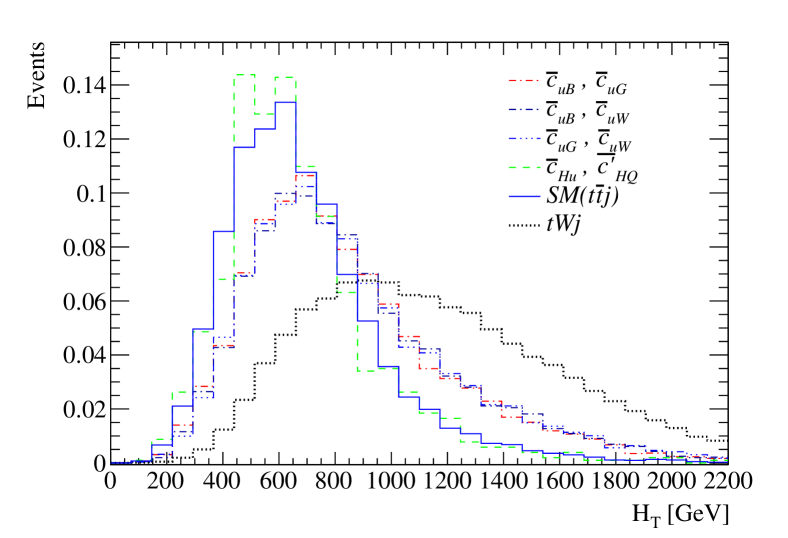
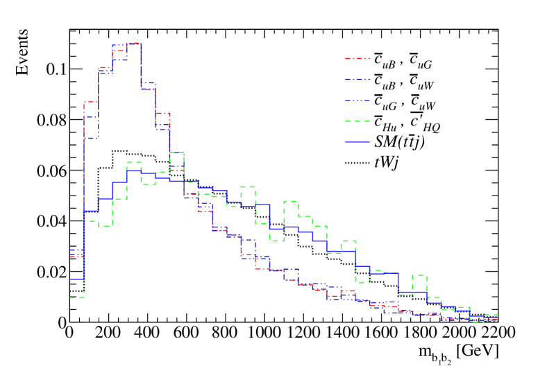
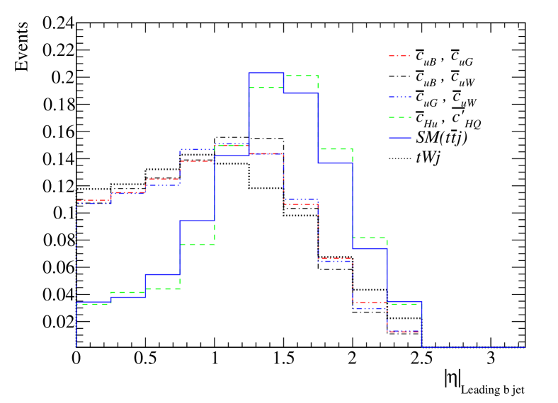
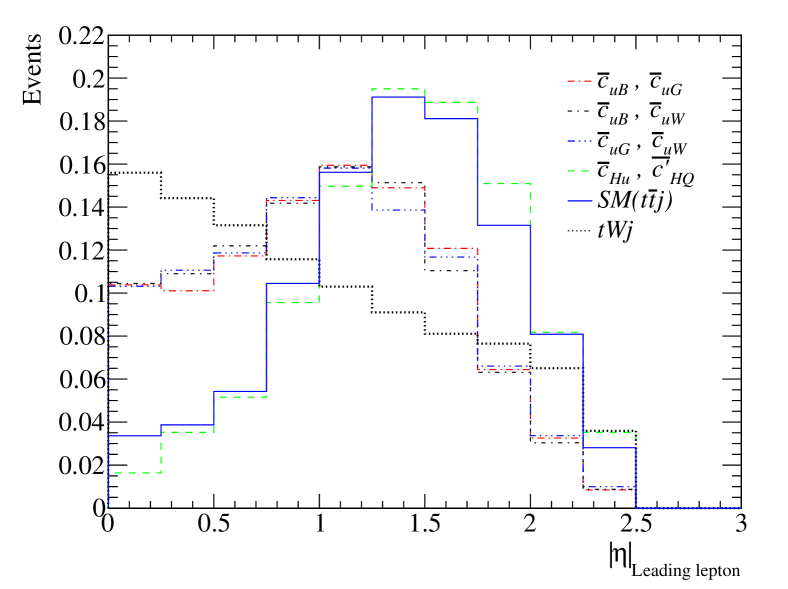
Figure 4: The normalised distributions of some of the input variables to the multivariate analysis. The plots show distributions of $H_{T}$ (top left), invariant mass of b-jets (top right) pseudorapidity of leading b-jet (bottom left) and leading lepton (bottom right) at $\sqrt{s}=$ 3000 GeV.

For instance, the BDTG output distribution for the signal scenario of $\bar{c}_{uB}=\bar{c}_{uG}=0.1$ is shown in Fig.5. Contrary to the overwhelming contribution of backgrounds, the gradient BDT performs well. The output of BDTG has been checked in terms of the power of discrimination from the receiver operator characteristic (ROC) of the output of BDTG output. The optimum cut on the BDTG response is chosen so that the best sensitivity is achieved.

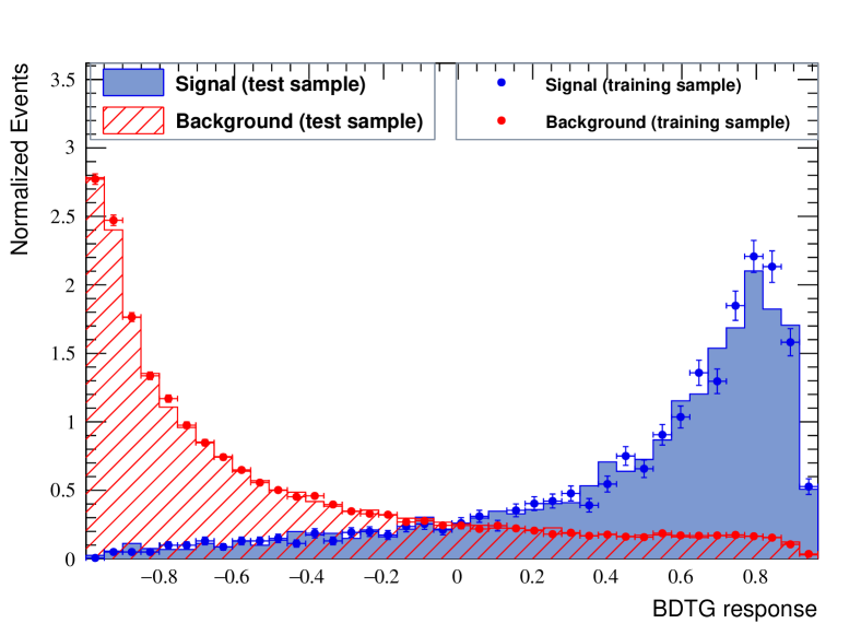
Figure 5: The distribution of the gradient BDT output for the signal with $c_{uB}=c_{uG}=0.1$ and for the SM backgrounds at the the center-of-mass energy of 3000 GeV.

Separate analyses are performed at the center-of-mass energies of 500 and 3000 GeV. The signal and background cross sections at $\sqrt{s}=3000$ GeV after performing the multivariate analysis are given in Table 1 for the signal scenario with $\bar{c}_{uW}=\bar{c}_{uB}=0.1$. As we can see from Table 1, the main background contributions come from the $tWj$ and $t\bar{t}+$jet processes.

$\sqrt{s}=3000$ GeV	Couplings	Signal	$t\bar{t}+$jet	$tWj$	$WWV+ZZV$	$VVV^{\prime}V^{\prime}$
MVA	$(\bar{c}_{uW},\bar{c}_{uB})$	4.42	0.0021	0.0041	0.0005	0.000043
$\sqrt{s}=500$ GeV	Couplings	Signal	$t\bar{t}+$jet	$tWj$	$WWV+ZZV$	$VVV^{\prime}V^{\prime}$
MVA	$(\bar{c}_{uW},\bar{c}_{uB})$	247.5	3.6	0.17	0.03	0.000023

Table 1: Expected cross sections of signal and background processes at $\sqrt{s}=500$ and 3000 GeV after performing the multivariate analysis. The signal cross section is presented for $\bar{c}_{uB}=\bar{c}_{uW}=0.1$ in the unit of fb.

We note that the considered operators affect the background processes. In this work, after the cuts and multivariate analysis, backgrounds are suppressed remarkably and the impacts of the included dimension six operators on the backgrounds are not sizeable. For instance, the change in the cross section of the $tWj$ background at $\sqrt{s}=500$ GeV in different scenarios are as follows:

$$\Delta\sigma_{tWj} = \sigma_{tWj}(\bar{c}_{uW}=0.1,\bar{c}_{uG}=0.1)-\sigma_{tWj}(0.0,0.0)=0.632$$

$$\Delta\sigma_{tWj} = \sigma_{tWj}(\bar{c}_{uW}=0.1,\bar{c}_{uB}=0.1)-\sigma_{tWj}(0.0,0.0)=0.637$$

$$\Delta\sigma_{tWj} = \sigma_{tWj}(\bar{c}_{uB}=0.1,\bar{c}_{uG}=0.1)-\sigma_{tWj}(0.0,0.0)=3.9\times 10^{-3},$$ (7)

the numbers are given in the unit of fb. The impact of the other operators on $tWj$ is quite negligible. The deviations that other background processes receive from the operators are not considerable and are found to be of the order of $\lesssim 10^{-4,-5}$ fb. In this analysis, we consider the impact of operators on the $tWj$ background when limits are set on the Wilson coefficients. The results and sensitivity estimation will be presented in the next section.

4 Results and discussions

In this section, we present the sensitivity of the future lepton colliders to the coefficients of dimension-six operators that could be obtained at the center-of-mass energies of 500 and 3000 GeV. We present the expected bounds at $95\%$ CL on the individual operators as well as marginalised limits over all contributing operators. Two-dimensional contours of the expected constraints at $95\%$ CL are presented in Fig.6 and Fig.7 for the center-of-mass energies of 3000 GeV and 500 GeV, respectively. The results at $\sqrt{s}=3000$ GeV are presented for two integrated luminosities of 300 and 3000 fb^-1.

As expected among the Wilson coefficients, the highest sensitivity belongs to $\bar{c}_{uW}$ then to $\bar{c}_{uB}$ so that at $\sqrt{s}=3$ TeV with 3 ab^-1 of data, one could probe them down to $10^{-3}$. In order to investigate how far these sensitivities are changed with including uncertainties, we also present the contours at $95\%$ CL by considering $10\%$ uncertainty on the cross sections of the background processes and a total $10\%$ uncertainty on the efficiency of signal. This would loosen the constraints up to around $15\%$.

The numerical one dimensional constraints at $95\%$ CL on the Wilson coefficients at both center-of-mass energies of 500 and 3000 GeV are given in Table 2.

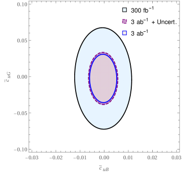
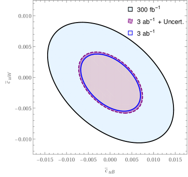
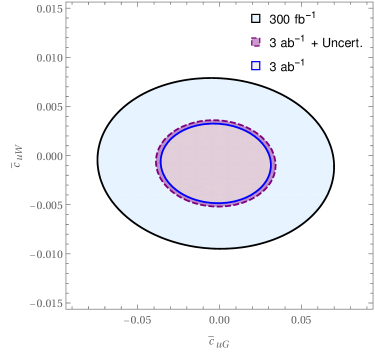
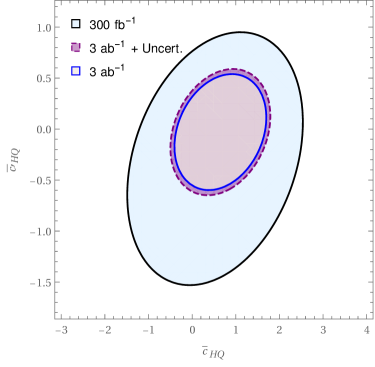
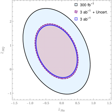
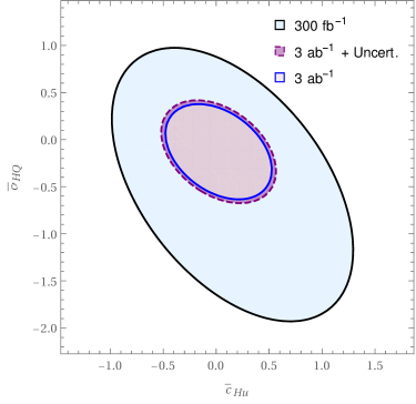
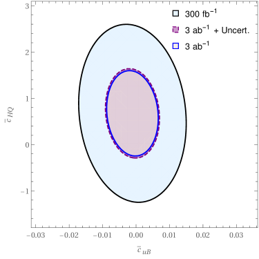
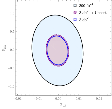
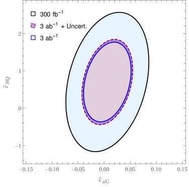
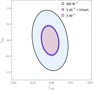
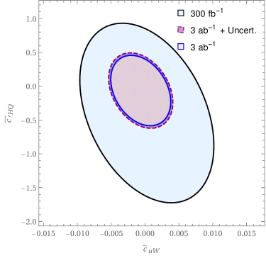
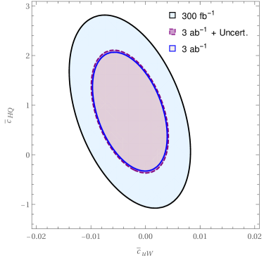
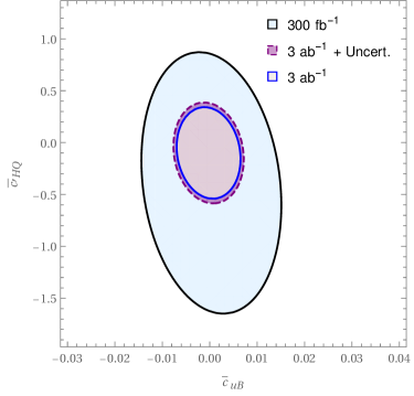
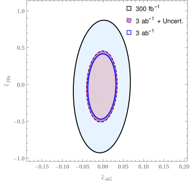
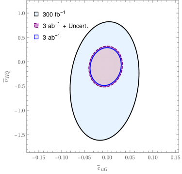
Figure 6: Contours of 95% CL at center-of-mass energy of 3000 GeV with the integrated luminosities of 300 and 3000 fb^-1. The contours of 95% CL considering an uncertainty of $10\%$ on the background rates and $10\%$ uncertainty on the signal efficiency with 3000 fb^-1.

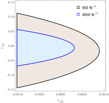
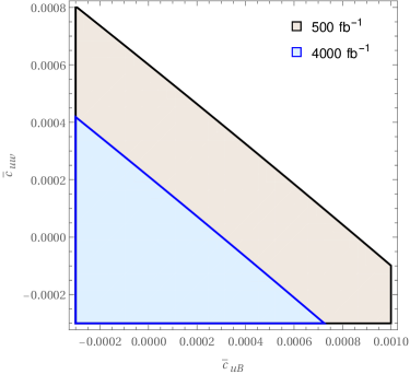
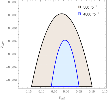
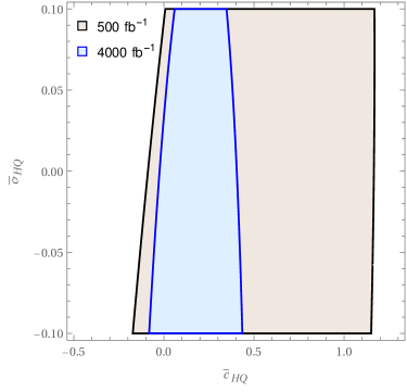
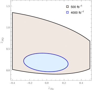
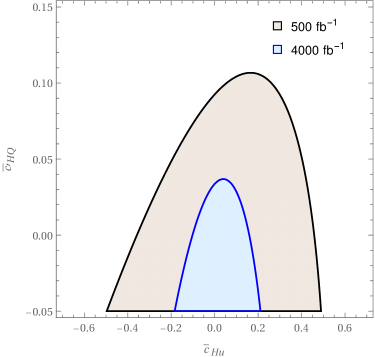
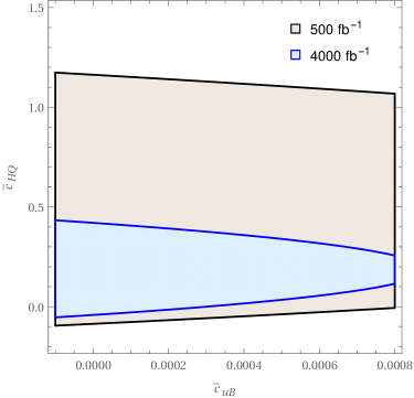
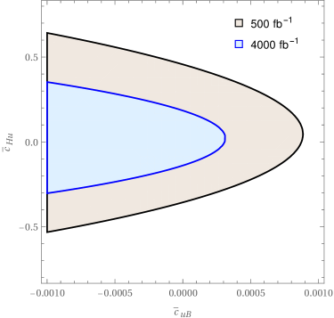
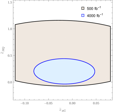
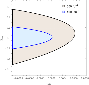
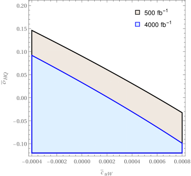
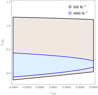
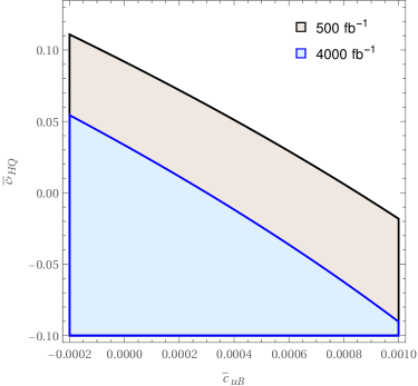
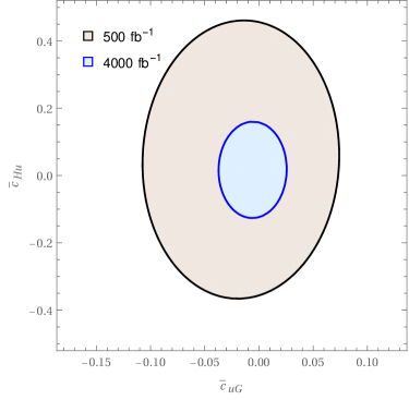
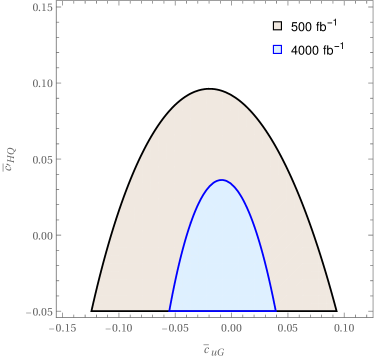
Figure 7: Contours of 95% confidence level at center-of-mass energy of 500 GeV with the integrated luminosities of 500 fb^-1 and 4000 fb^-1. Some plots are magnified for better clarity.

Table 2: The $95\%$ CL constraints on the Wilson coefficients for different assumptions on the integrated luminosity at the center-of-mass energies of 500 and 3000 GeV.

Wilson coefficient	$500$ GeV, 500 fb-1	$500$ GeV, 4 ab-1	$3$ TeV, 300 fb-1	$3$ TeV, 3 ab-1
$\bar{c}_{uB}$	$[-0.0476,0.0009]$	$[-0.017,0.0003]$	$[-0.013,0.012]$	$[-0.0067,0.0058]$
$\bar{c}_{uG}$	$[-0.11,0.073]$	$[-0.039,0.025]$	$[-0.073,0.068]$	$[-0.038,0.033]$
$\bar{c}_{uW}$	$[-0.0294,0.0006]$	$[-0.011,0.0002]$	$[-0.0098,0.0082]$	$[-0.0051,0.0035]$
$\bar{c}_{Hu}$	$[-0.35,0.45]$	$[-0.12,0.16]$	$[-1.00,0.95]$	$[-0.51,0.46]$
$\bar{c}_{HQ}$	$[-0.087,1.17]$	$[-0.032,0.41]$	$[-1.21,2.53]$	$[-0.37,1.69]$
$\bar{c}^{\prime}_{HQ}$	$[-1.34,0.093]$	$[-0.48,0.034]$	$[-1.63,0.86]$	$[-0.54,0.31]$

From Table 2, we see that the limits derived from the analysis of 3 ab^-1 of data from electron-positron collisions at $\sqrt{s}=3$ TeV on the $\bar{c}_{uW}$ and $\bar{c}_{uB}$ are at the level of $10^{-3}$, respectively. For $\sqrt{s}=500$ GeV, $\bar{c}_{uW}$ and $\bar{c}_{uB}$ reach one order better sensitivity with the integrated luminosities of 500 fb^-1 and 4000 fb^-1.

With the assumption of $c_{X}=1$, the bound on $\bar{c}_{uW}$ (from $\sqrt{s}=500$ GeV with 4000 fb^-1) corresponds to a mass scale of $\Lambda\gtrsim 17$ TeV. The validity of the effective theory is determined by the energy scale of the process which is fixed at lepton colliders and is equal to the center-of-mass energy. The obtained constraints from this analysis are larger than the energy scale of the interaction, i.e. $\Lambda>\sqrt{s}$, which is consistent with the EFT description. The $\mathcal{O}_{uW}$ and $\mathcal{O}_{uB}$ operators have been probed using the $t\bar{t}$ production in Ref.[75] for various scenarios at the CLIC and ILC. It has been shown that using observables such as total cross section, forward-backward asymmetries, and utilising different sets of beam polarisation would lead to constraints on $\bar{c}_{uW}$ and $\bar{c}_{uB}$ at the order of $\lesssim 10^{-4}$. The results from this analysis derives comparable bounds on $\mathcal{O}_{uW}$ and $\mathcal{O}_{uB}$ operators with those from Ref.[75]. We note that combining the semi-leptonic topology of $t\bar{t}j$ process with the dileptonic one, considered in this analysis, would improve the bounds.

The derived limits in this analysis could be used to probe the parameters of explicit models which their low energy limits tend to the SMEFT. For instance, in beyond the SM scenarios with strongly interacting Higgs boson, a naive estimation leads to the following for the Wilson coefficients [74, 99]:

$$\bar{c}_{uW},~{}\bar{c}_{uB},~{}\bar{c}_{uG}\sim\mathcal{O}\big{(}\frac{g^{*2}m_{W}^{2}}{16\pi^{2}M^{2}}\big{)}.$$ (8)

where $M$ is the mass scale of the new physical state and $g^{*}(\leq 4\pi)$ denotes the coupling strength of the Higgs boson to the new physics state. The obtained limit on $\bar{c}_{uW}$ at $\sqrt{s}=3$ TeV with 3 ab^-1 integrated luminosity of data lead to a lower bound of $7$ TeV on $M$, in the strongly interacting regime $g^{*}=4\pi$.

5 Summary and conclusions

We perform a study to probe the sensitivity of future lepton colliders to the top quark effective couplings at the center-of-mass energies of 500 and 3000 GeV. In particular, we concentrate on the top pair production in association with a jet within the SMEFT framework. The SMEFT is an attractive and an efficient way to describe the possible effects of new physics until new particles from beyond the SM are observed. The $e^{-}e^{+}\rightarrow t\bar{t}$+jet process is found to be mostly sensitive to $\mathcal{O}_{uW}$ and $\mathcal{O}_{uB}$ operators, respectively. The clean environment at lepton colliders and the expected high resolution for measurements of leptons and jets properties allow us to characterise the $t\bar{t}+$jet events through the dileptonic channel, where the final state consists of two charged lepton ($\ell^{\pm}$), at least two jets from which two are originating from hadronisation of $b$-quarks, and missing transverse momentum. The results are based on a comprehensive analysis where the major sources of background processes and a realistic simulation of the detector response, flavour tagging, and jet clustering have been considered. A set of kinematic variables consisting of scalar sum of the transverse momentum of the leptons and jets, invariant mass of the b-jets, and pseudorapidity of the leading lepton and b-jet are used as input to a multivariate analysis for separation of signal from background processes.

It is found that using lepton colliders at both center-of-mass energies $\sqrt{s}=3000$ and 500 GeV would allow us to constrain the $\bar{c}_{uW}$ and $\bar{c}_{uB}$ of the order of $10^{-3}$ and $10^{-4}$, respectively.

References

- [1] G. Aad et al. [ATLAS Collaboration], “Observation of a new particle in the search for the Standard Model Higgs boson with the ATLAS detector at the LHC,” Phys. Lett. B 716, 1 (2012) doi:10.1016/j.physletb.2012.08.020 [arXiv:1207.7214 [hep-ex]].
- [2] S. Chatrchyan et al. [CMS Collaboration], “Observation of a New Boson at a Mass of 125 GeV with the CMS Experiment at the LHC,” Phys. Lett. B 716, 30 (2012) doi:10.1016/j.physletb.2012.08.021 [arXiv:1207.7235 [hep-ex]].
- [3] S. Dawson et al., “Working Group Report: Higgs Boson,” arXiv:1310.8361 [hep-ex].
- [4] D. de Florian et al. [LHC Higgs Cross Section Working Group], “Handbook of LHC Higgs Cross Sections: 4. Deciphering the Nature of the Higgs Sector,” doi:10.23731/CYRM-2017-002 arXiv:1610.07922 [hep-ph].
- [5] S. Heinemeyer et al. [LHC Higgs Cross Section Working Group], “Handbook of LHC Higgs Cross Sections: 3. Higgs Properties,” doi:10.5170/CERN-2013-004 arXiv:1307.1347 [hep-ph].
- [6] F. Abe et al. [CDF Collaboration], “Observation of top quark production in collisions,” Phys. Rev. Lett. 74, 2626 (1995) doi:10.1103/PhysRevLett.74.2626 [hep-ex/9503002].
- [7] S. Abachi et al. [D0 Collaboration], “Search for high mass top quark production in collisions at TeV,” Phys. Rev. Lett. 74, 2422 (1995) doi:10.1103/PhysRevLett.74.2422 [hep-ex/9411001].
- [8] J. Fan, M. Reece and L. T. Wang, “Possible Futures of Electroweak Precision: ILC, FCC-ee, and CEPC,” JHEP 1509, 196 (2015) doi:10.1007/JHEP09(2015)196 [arXiv:1411.1054 [hep-ph]].
- [9] G. Moortgat-Pick et al., “Physics at the e+ e- Linear Collider,” Eur. Phys. J. C 75, no. 8, 371 (2015) doi:10.1140/epjc/s10052-015-3511-9 [arXiv:1504.01726 [hep-ph]].
- [10] K. Fujii et al., “Physics Case for the International Linear Collider,” arXiv:1506.05992 [hep-ex].
- [11] P. N. Burrows et al. [CLICdp and CLIC Collaborations], “The Compact Linear Collider (CLIC) - 2018 Summary Report,” CERN Yellow Rep. Monogr. 1802, 1 (2018) doi:10.23731/CYRM-2018-002 [arXiv:1812.06018 [physics.acc-ph]].
- [12] P. Roloff et al. [CLIC and CLICdp Collaborations], “The Compact Linear e+e- Collider (CLIC): Physics Potential,” arXiv:1812.07986 [hep-ex].
- [13] M. Aicheler et al. [CLIC accelerator Collaboration], “The Compact Linear Collider (CLIC) - Project Implementation Plan,” doi:10.23731/CYRM-2018-004 arXiv:1903.08655 [physics.acc-ph].
- [14] H. Aihara et al. [ILC Collaboration], “The International Linear Collider. A Global Project,” arXiv:1901.09829 [hep-ex].
- [15] H. Baer et al., “The International Linear Collider Technical Design Report - Volume 2: Physics,” arXiv:1306.6352 [hep-ph].
- [16] T. Behnke et al., “The International Linear Collider Technical Design Report - Volume 1: Executive Summary,” arXiv:1306.6327 [physics.acc-ph].
- [17] M. Ahmad et al., “CEPC-SPPC Preliminary Conceptual Design Report. 1. Physics and Detector,” IHEP-CEPC-DR-2015-01, IHEP-TH-2015-01, IHEP-EP-2015-01.
- [18] CEPC-SPPC Study Group, “CEPC-SPPC Preliminary Conceptual Design Report. 2. Accelerator,” IHEP-CEPC-DR-2015-01, IHEP-AC-2015-01.
- [19] A. Abada et al. [FCC Collaboration], “FCC-ee: The Lepton Collider : Future Circular Collider Conceptual Design Report Volume 2,” Eur. Phys. J. ST 228, no. 2, 261 (2019). doi:10.1140/epjst/e2019-900045-4
- [20] M. Bicer et al. [TLEP Design Study Working Group], “First Look at the Physics Case of TLEP,” JHEP 1401, 164 (2014) doi:10.1007/JHEP01(2014)164 [arXiv:1308.6176 [hep-ex]].
- [21] A. Abada et al. [FCC Collaboration], “FCC Physics Opportunities : Future Circular Collider Conceptual Design Report Volume 1,” Eur. Phys. J. C 79, no. 6, 474 (2019). doi:10.1140/epjc/s10052-019-6904-3
- [22] A. Abada et al. [FCC Collaboration], “FCC-ee: The Lepton Collider : Future Circular Collider Conceptual Design Report Volume 2,” Eur. Phys. J. ST 228, no. 2, 261 (2019). doi:10.1140/epjst/e2019-900045-4
- [23] P. Azzi et al. [HL-LHC Collaboration and HE-LHC Working Group], “Standard Model Physics at the HL-LHC and HE-LHC,” arXiv:1902.04070 [hep-ph].
- [24] J. Beacham et al., “Physics Beyond Colliders at CERN: Beyond the Standard Model Working Group Report,” arXiv:1901.09966 [hep-ex].
- [25] X. Cid Vidal et al. [Working Group 3], “Beyond the Standard Model Physics at the HL-LHC and HE-LHC,” arXiv:1812.07831 [hep-ph].
- [26] F. Maltoni, L. Mantani and K. Mimasu, “Top-quark electroweak interactions at high energy,” arXiv:1904.05637 [hep-ph].
- [27] C. W. Murphy, “Statistical approach to Higgs boson couplings in the standard model effective field theory,” Phys. Rev. D 97, no. 1, 015007 (2018) doi:10.1103/PhysRevD.97.015007 [arXiv:1710.02008 [hep-ph]].
- [28] G. Durieux, M. Perello, M. Vos and C. Zhang, “Global and optimal probes for the top-quark effective field theory at future lepton colliders,” JHEP 1810, 168 (2018) doi:10.1007/JHEP10(2018)168 [arXiv:1807.02121 [hep-ph]].
- [29] G. Durieux, J. Gu, E. Vryonidou and C. Zhang, “Probing top-quark couplings indirectly at Higgs factories,” Chin. Phys. C 42, no. 12, 123107 (2018) doi:10.1088/1674-1137/42/12/123107 [arXiv:1809.03520 [hep-ph]].
- [30] G. Durieux, A. Irles, V. Miralles, A. Penuelas, R. Poschl, M. Perello and M. Vos, “The electro-weak couplings of the top and bottom quarks – global fit and future prospects,” arXiv:1907.10619 [hep-ph].
- [31] M. Chala, J. Santiago and M. Spannowsky, “Constraining four-fermion operators using rare top decays,” JHEP 1904, 014 (2019) doi:10.1007/JHEP04(2019)014 [arXiv:1809.09624 [hep-ph]].
- [32] C. Englert, R. Kogler, H. Schulz and M. Spannowsky, “Higgs coupling measurements at the LHC,” Eur. Phys. J. C 76, no. 7, 393 (2016) doi:10.1140/epjc/s10052-016-4227-1 [arXiv:1511.05170 [hep-ph]].
- [33] J. A. Aguilar-Saavedra et al., “Interpreting top-quark LHC measurements in the standard-model effective field theory,” arXiv:1802.07237 [hep-ph].
- [34] I. Brivio and M. Trott, “The Standard Model as an Effective Field Theory,” Phys. Rept. 793, 1 (2019) doi:10.1016/j.physrep.2018.11.002 [arXiv:1706.08945 [hep-ph]].
- [35] I. Brivio, T. Corbett and M. Trott, “The Higgs width in the SMEFT,” arXiv:1906.06949 [hep-ph].
- [36] H. Khanpour and M. Mohammadi Najafabadi, “Constraining Higgs boson effective couplings at electron-positron colliders,” Phys. Rev. D 95, no. 5, 055026 (2017) doi:10.1103/PhysRevD.95.055026 [arXiv:1702.00951 [hep-ph]].
- [37] H. Hesari, H. Khanpour and M. Mohammadi Najafabadi, “Study of Higgs Effective Couplings at Electron-Proton Colliders,” Phys. Rev. D 97, no. 9, 095041 (2018) doi:10.1103/PhysRevD.97.095041 [arXiv:1805.04697 [hep-ph]].
- [38] H. Khanpour, S. Khatibi and M. Mohammadi Najafabadi, “Probing Higgs boson couplings in H+ production at the LHC,” Phys. Lett. B 773, 462 (2017) doi:10.1016/j.physletb.2017.09.005 [arXiv:1702.05753 [hep-ph]].
- [39] J. Ellis and T. You, “Sensitivities of Prospective Future e+e- Colliders to Decoupled New Physics,” JHEP 1603, 089 (2016) doi:10.1007/JHEP03(2016)089 [arXiv:1510.04561 [hep-ph]].
- [40] W. H. Chiu, S. C. Leung, T. Liu, K. F. Lyu and L. T. Wang, “Probing 6D operators at future e?e+ colliders,” JHEP 1805, 081 (2018) doi:10.1007/JHEP05(2018)081 [arXiv:1711.04046 [hep-ph]].
- [41] J. Ellis, P. Roloff, V. Sanz and T. You, “Dimension-6 Operator Analysis of the CLIC Sensitivity to New Physics,” JHEP 1705, 096 (2017) doi:10.1007/JHEP05(2017)096 [arXiv:1701.04804 [hep-ph]].
- [42] G. Brooijmans et al., “Les Houches 2015: Physics at TeV colliders - new physics working group report,” arXiv:1605.02684 [hep-ph].
- [43] R. Rontsch and M. Schulze, “Probing top-Z dipole moments at the LHC and ILC,” JHEP 1508, 044 (2015) doi:10.1007/JHEP08(2015)044 [arXiv:1501.05939 [hep-ph]].
- [44] R. Rontsch and M. Schulze, “Constraining couplings of top quarks to the Z boson in + Z production at the LHC,” JHEP 1407, 091 (2014) Erratum: [JHEP 1509, 132 (2015)] doi:10.1007/JHEP09(2015)132, 10.1007/JHEP07(2014)091 [arXiv:1404.1005 [hep-ph]].
- [45] G. Durieux, C. Grojean, J. Gu and K. Wang, “The leptonic future of the Higgs,” JHEP 1709, 014 (2017) doi:10.1007/JHEP09(2017)014 [arXiv:1704.02333 [hep-ph]].
- [46] A. Buckley, C. Englert, J. Ferrando, D. J. Miller, L. Moore, M. Russell and C. D. White, “Constraining top quark effective theory in the LHC Run II era,” JHEP 1604, 015 (2016) doi:10.1007/JHEP04(2016)015 [arXiv:1512.03360 [hep-ph]].
- [47] A. Buckley, C. Englert, J. Ferrando, D. J. Miller, L. Moore, M. Russell and C. D. White, “Global fit of top quark effective theory to data,” Phys. Rev. D 92, no. 9, 091501 (2015) doi:10.1103/PhysRevD.92.091501 [arXiv:1506.08845 [hep-ph]].
- [48] M. S. Amjad et al., “A precise determination of top quark electro-weak couplings at the ILC operating at GeV,” arXiv:1307.8102 [hep-ex].
- [49] M. Baak et al. [Gfitter Group], “The global electroweak fit at NNLO and prospects for the LHC and ILC,” Eur. Phys. J. C 74, 3046 (2014) doi:10.1140/epjc/s10052-014-3046-5 [arXiv:1407.3792 [hep-ph]].
- [50] I. Brivio, Y. Jiang and M. Trott, “The SMEFTsim package, theory and tools,” JHEP 1712, 070 (2017) doi:10.1007/JHEP12(2017)070 [arXiv:1709.06492 [hep-ph]].
- [51] A. Vasquez, C. Degrande, A. Tonero and R. Rosenfeld, “New physics in double Higgs production at future e+e? colliders,” JHEP 1905, 020 (2019) doi:10.1007/JHEP05(2019)020 [arXiv:1901.05979 [hep-ph]].
- [52] D. Atwood, S. Bar-Shalom, G. Eilam and A. Soni, “CP violation in top physics,” Phys. Rept. 347, 1 (2001) doi:10.1016/S0370-1573(00)00112-5 [hep-ph/0006032].
- [53] C. Englert, A. Freitas, M. M. Muhlleitner, T. Plehn, M. Rauch, M. Spira and K. Walz, “Precision Measurements of Higgs Couplings: Implications for New Physics Scales,” J. Phys. G 41, 113001 (2014), [arXiv:1403.7191 [hep-ph]].
- [54] J. A. Aguilar-Saavedra, B. Fuks and M. L. Mangano, “Pinning down top dipole moments with ultra-boosted tops,” Phys. Rev. D 91, 094021 (2015) doi:10.1103/PhysRevD.91.094021 [arXiv:1412.6654 [hep-ph]].
- [55] M. Mohammadi Najafabadi, “Probing of Wtb Anomalous Couplings via the tW Channel of Single Top Production,” JHEP 0803, 024 (2008) doi:10.1088/1126-6708/2008/03/024 [arXiv:0801.1939 [hep-ph]].
- [56] J. Ellis, V. Sanz and T. You, “The Effective Standard Model after LHC Run I,” JHEP 1503, 157 (2015) doi:10.1007/JHEP03(2015)157 [arXiv:1410.7703 [hep-ph]].
- [57] C. Englert, R. Kogler, H. Schulz and M. Spannowsky, “Higgs coupling measurements at the LHC,” Eur. Phys. J. C 76, no. 7, 393 (2016) doi:10.1140/epjc/s10052-016-4227-1 [arXiv:1511.05170 [hep-ph]].
- [58] J. Ellis, V. Sanz and T. You, “Complete Higgs Sector Constraints on Dimension-6 Operators,” JHEP 1407, 036 (2014) doi:10.1007/JHEP07(2014)036 [arXiv:1404.3667 [hep-ph]].
- [59] H. Denizli and A. Senol, “Constraints on Higgs effective couplings in production of CLIC at 380 GeV,” Adv. High Energy Phys. 2018, 1627051 (2018) doi:10.1155/2018/1627051 [arXiv:1707.03890 [hep-ph]].
- [60] H. Denizli, K. Y. Oyulmaz and A. Senol, “Testing for observability of Higgs effective couplings in triphoton production at FCC-hh,” arXiv:1901.04784 [hep-ph].
- [61] H. Hesari, “Probing Higgs boson couplings in production at the LHC,” arXiv:1807.04306 [hep-ph].
- [62] J. A. Dror, M. Farina, E. Salvioni and J. Serra, “Strong tW Scattering at the LHC,” JHEP 1601, 071 (2016) doi:10.1007/JHEP01(2016)071 [arXiv:1511.03674 [hep-ph]].
- [63] C. Hartmann, W. Shepherd and M. Trott, “The decay width in the SMEFT: and corrections at one loop,” JHEP 1703, 060 (2017) doi:10.1007/JHEP03(2017)060 [arXiv:1611.09879 [hep-ph]].
- [64] S. Fichet, A. Tonero and P. Rebello Teles, “Sharpening the shape analysis for higher-dimensional operator searches,” Phys. Rev. D 96, no. 3, 036003 (2017) doi:10.1103/PhysRevD.96.036003 [arXiv:1611.01165 [hep-ph]].
- [65] L. Berthier and M. Trott, “Consistent constraints on the Standard Model Effective Field Theory,” JHEP 1602, 069 (2016) doi:10.1007/JHEP02(2016)069 [arXiv:1508.05060 [hep-ph]].
- [66] G. Durieux, M. Perelló, M. Vos and C. Zhang, “Global and optimal probes for the top-quark effective field theory at future lepton colliders,” JHEP 1810, 168 (2018) doi:10.1007/JHEP10(2018)168 [arXiv:1807.02121 [hep-ph]].
- [67] P. Artoisenet et al., “A framework for Higgs characterisation,” JHEP 1311, 043 (2013) doi:10.1007/JHEP11(2013)043 [arXiv:1306.6464 [hep-ph]].
- [68] A. Alloul, B. Fuks and V. Sanz, “Phenomenology of the Higgs Effective Lagrangian via FEYNRULES,” JHEP 1404, 110 (2014) doi:10.1007/JHEP04(2014)110 [arXiv:1310.5150 [hep-ph]].
- [69] W. Buchmuller and D. Wyler, “Effective Lagrangian Analysis of New Interactions and Flavor Conservation,” Nucl. Phys. B 268, 621 (1986). doi:10.1016/0550-3213(86)90262-2
- [70] B. Grzadkowski, M. Iskrzynski, M. Misiak and J. Rosiek, “Dimension-Six Terms in the Standard Model Lagrangian,” JHEP 1010, 085 (2010) doi:10.1007/JHEP10(2010)085 [arXiv:1008.4884 [hep-ph]].
- [71] K. Hagiwara, S. Ishihara, R. Szalapski and D. Zeppenfeld, “Low-energy effects of new interactions in the electroweak boson sector,” Phys. Rev. D 48, 2182 (1993). doi:10.1103/PhysRevD.48.2182
- [72] G. Buchalla, O. Cata and C. Krause, “A Systematic Approach to the SILH Lagrangian,” Nucl. Phys. B 894, 602 (2015) doi:10.1016/j.nuclphysb.2015.03.024 [arXiv:1412.6356 [hep-ph]].
- [73] G. Buchalla, O. Cata, A. Celis and C. Krause, “Note on Anomalous Higgs-Boson Couplings in Effective Field Theory,” Phys. Lett. B 750, 298 (2015) doi:10.1016/j.physletb.2015.09.027 [arXiv:1504.01707 [hep-ph]].
- [74] R. Contino, M. Ghezzi, C. Grojean, M. Muhlleitner and M. Spira, “Effective Lagrangian for a light Higgs-like scalar,” JHEP 1307, 035 (2013) doi:10.1007/JHEP07(2013)035 [arXiv:1303.3876 [hep-ph]].
- [75] C. Englert and M. Russell, “Top quark electroweak couplings at future lepton colliders,” Eur. Phys. J. C 77, no. 8, 535 (2017) doi:10.1140/epjc/s10052-017-5095-z [arXiv:1704.01782 [hep-ph]].
- [76] A. M. Sirunyan et al. [CMS Collaboration], “Measurement of the cross section for top quark pair production in association with a W or Z boson in proton-proton collisions at 13 TeV,” JHEP 1808, 011 (2018) doi:10.1007/JHEP08(2018)011 [arXiv:1711.02547 [hep-ex]].
- [77] [CMS Collaboration], “Measurement of top quark pair production in association with a Z boson in proton-proton collisions at 13 TeV,” arXiv:1907.11270 [hep-ex].
- [78] N. P. Hartland, F. Maltoni, E. R. Nocera, J. Rojo, E. Slade, E. Vryonidou and C. Zhang, “A Monte Carlo global analysis of the Standard Model Effective Field Theory: the top quark sector,” JHEP 1904, 100 (2019) doi:10.1007/JHEP04(2019)100 [arXiv:1901.05965 [hep-ph]].
- [79] I. Brivio, S. Bruggisser, F. Maltoni, R. Moutafis, T. Plehn, E. Vryonidou, S. Westhoff and C. Zhang, “O new physics, where art thou? A global search in the top sector,” arXiv:1910.03606 [hep-ph].
- [80] J. Ellis, C. W. Murphy, V. Sanz and T. You, JHEP 1806, 146 (2018) doi:10.1007/JHEP06(2018)146 [arXiv:1803.03252 [hep-ph]].
- [81] J. Alwall, M. Herquet, F. Maltoni, O. Mattelaer and T. Stelzer, “MadGraph 5 : Going Beyond,” JHEP 1106, 128 (2011) doi:10.1007/JHEP06(2011)128 [arXiv:1106.0522 [hep-ph]].
- [82] J. Alwall, C. Duhr, B. Fuks, O. Mattelaer, D. G. Ozturk and C. H. Shen, “Computing decay rates for new physics theories with FeynRules and MadGraph 5_aMC@NLO,” Comput. Phys. Commun. 197, 312 (2015) doi:10.1016/j.cpc.2015.08.031 [arXiv:1402.1178 [hep-ph]].
- [83] J. Alwall et al., “The automated computation of tree-level and next-to-leading order differential cross sections, and their matching to parton shower simulations,” JHEP 1407, 079 (2014) doi:10.1007/JHEP07(2014)079 [arXiv:1405.0301 [hep-ph]].
- [84] A. Alloul, N. D. Christensen, C. Degrande, C. Duhr and B. Fuks, “FeynRules 2.0 - A complete toolbox for tree-level phenomenology,” Comput. Phys. Commun. 185, 2250 (2014) doi:10.1016/j.cpc.2014.04.012 [arXiv:1310.1921 [hep-ph]].
- [85] C. Degrande, C. Duhr, B. Fuks, D. Grellscheid, O. Mattelaer and T. Reiter, “UFO - The Universal FeynRules Output,” Comput. Phys. Commun. 183, 1201 (2012) doi:10.1016/j.cpc.2012.01.022 [arXiv:1108.2040 [hep-ph]].
- [86] M. L. Mangano, M. Moretti, F. Piccinini and M. Treccani, “Matching matrix elements and shower evolution for top-quark production in hadronic collisions,” JHEP 0701, 013 (2007) doi:10.1088/1126-6708/2007/01/013 [hep-ph/0611129].
- [87] M. Tanabashi et al. [Particle Data Group], “Review of Particle Physics,” Phys. Rev. D 98, no. 3, 030001 (2018). doi:10.1103/PhysRevD.98.030001
- [88] T. Sjostrand et al., “An Introduction to PYTHIA 8.2,” Comput. Phys. Commun. 191, 159 (2015) doi:10.1016/j.cpc.2015.01.024 [arXiv:1410.3012 [hep-ph]].
- [89] T. Sjostrand, S. Mrenna and P. Z. Skands, “A Brief Introduction to PYTHIA 8.1,” Comput. Phys. Commun. 178, 852 (2008) doi:10.1016/j.cpc.2008.01.036 [arXiv:0710.3820 [hep-ph]].
- [90] J. de Favereau et al. [DELPHES 3 Collaboration], “DELPHES 3, A modular framework for fast simulation of a generic collider experiment,” JHEP 1402, 057 (2014) doi:10.1007/JHEP02(2014)057 [arXiv:1307.6346 [hep-ex]].
- [91] T. Behnke et al., “The International Linear Collider Technical Design Report - Volume 4: Detectors,” arXiv:1306.6329 [physics.ins-det].
- [92] M. Cacciari, G. P. Salam and G. Soyez, “The anti- jet clustering algorithm,” JHEP 0804, 063 (2008) doi:10.1088/1126-6708/2008/04/063 [arXiv:0802.1189 [hep-ph]].
- [93] M. Cacciari, G. P. Salam and G. Soyez, “FastJet User Manual,” Eur. Phys. J. C 72, 1896 (2012) doi:10.1140/epjc/s10052-012-1896-2 [arXiv:1111.6097 [hep-ph]].
- [94] A. Hocker et al., “TMVA - Toolkit for Multivariate Data Analysis,” PoS ACAT , 040 (2007) [physics/0703039 [PHYSICS]].
- [95] J. Stelzer, A. Hocker, P. Speckmayer and H. Voss, “Current developments in TMVA: An outlook to TMVA4,” PoS ACAT 08, 063 (2008).
- [96] J. Therhaag [TMVA Core Developer Team Collaboration], “TMVA: Toolkit for multivariate data analysis,” AIP Conf. Proc. 1504, 1013 (2009).
- [97] P. Speckmayer, A. Hocker, J. Stelzer and H. Voss, “The toolkit for multivariate data analysis, TMVA 4,” J. Phys. Conf. Ser. 219, 032057 (2010).
- [98] J. Therhaag, “TMVA Toolkit for multivariate data analysis in ROOT,” PoS ICHEP 2010, 510 (2010).
- [99] G. F. Giudice, C. Grojean, A. Pomarol and R. Rattazzi, “The Strongly-Interacting Light Higgs,” JHEP 0706, 045 (2007) doi:10.1088/1126-6708/2007/06/045 [hep-ph/0703164].