Energy-preserving exponential integrable numerical method for stochastic cubic wave equation with additive noise

Abstract

In this paper, we present an energy-preserving exponentially integrable numerical method for stochastic wave equation with cubic nonlinearity and additive noise. We first apply the spectral Galerkin method to discretizing the original equation and show that this spatial discretization possesses an energy evolution law and certain exponential integrability property. Then the exponential integrability property of the exact solution is deduced by proving the strong convergence of the semi-discretization. To propose a full discrete numerical method which could inherit both the energy evolution law and the exponential integrability, we use the splitting technique and averaged vector field method in the temporal direction. Combining these structure-preserving properties with regularity estimates of the exact and the numerical solutions, we obtain the strong convergence rate of the numerical method. Numerical experiments coincide with these theoretical results.

AMS subject classification: 60H08, 60H35, 65C30.

Key Words: stochastic wave equation, cubic nonlinearity, strong convergence, spectral Galerkin method, exponential integrability property, energy evolution law

1 Introduction

As a kind of commonly observed physical phenomena, the wave motions are usually described by stochastic partial differential equations (SPDEs) of hyperbolic type. The main objective of this paper is to numerically investigate the following stochastic wave equation with cubic nonlinearity, driven by an additive noise

$$\left\{\begin{aligned} &du(t)=v(t)dt,\quad\quad\;\;&\text{in}\;\;\mathcal{O}\times(0,T],\\ &dv(t)=\Lambda u(t)dt-f(u(t))dt+dW(t),\quad\quad\;\;&\text{in}\;\;\mathcal{O}\times(0,T],\\ &u(0)=u_{0},\quad v(0)=v_{0},\quad\;\;&\text{in}\;\;\mathcal{O},\end{aligned}\right.$$ (1)

where $\mathcal{O}=(0,1)^{d}$ with $d\leq 2$, $T\in(0,\infty)$ and $u_{0},v_{0}:\mathcal{O}\rightarrow\mathbb{R}$ are deterministic. Assume that $\Lambda=\sum\limits_{i=1}^{d}\frac{\partial^{2}}{\partial x_{i}^{2}}$ is the Laplace operator with homogeneous Dirichlet boundary condition, and the nonlinear term $f(u)=c_{3}u^{3}+\cdots+c_{1}u+c_{0}$ is assumed to be a polynomial with $c_{3}>0$. Throughout this paper, $W$ is an $L^{2}:=L^{2}(\mathcal{O};\mathbb{R})$-valued $\mathbf{Q}$-Wiener process with respect to a filtered probability space $(\Omega,\mathcal{F},\{\mathcal{F}_{t}\}_{t\geq 0},\mathbb{P})$, i.e., there exists an orthonormal basis $\{e_{k}\}_{k\in\mathbb{N}^{+}}$ of $L^{2}$ and a sequence of mutually independent real-valued Brownian motions $\{\beta_{k}\}_{k\in\mathbb{N}^{+}}$ such that $W(x,t)=\sum_{k\in\mathbb{N}^{+}}\mathbf{Q}^{\frac{1}{2}}e_{k}(x)\beta_{k}(t)$ with $\mathbf{Q}$ being a symmetric, positive definite and finite trace operator. For the well-posedness of stochastic wave equation, we refer to [6, 7] for the existence and uniqueness of the mild solution with more general polynomial drift coefficients, and to [15] with more general driving noises. The evolution of the energy, as an intrinsic quantity of the wave equation, is studied in [6]. As another important property (see e.g., [1]), the exponential integrability property of the solution of the stochastic wave equation has not been well understood. We are only aware that the authors in [9] prove the exponential integrability property of the spectral Galerkin approximation of $2$-dimensional stochastic wave equation. Utilizing the uniform exponential integrability property and regularity estimate of the spectral Galerkin method applied to (LABEL:mod;swe), in this paper we prove that the exact solution admits the following exponential integrability property

$$\mathbb{E}\left(\exp\left(\int_{0}^{T}c\|u(s)\|_{L^{6}}^{2}ds\right)\right)\leq C,$$

where $c\in\mathbb{R}$, $T\in(0,\infty)$, $C:=C(u_{0},v_{0},\mathbf{Q},T,c,d)$ and $d\leq 2.$

Finding solutions numerically of stochastic wave equation is an active ongoing research area. For instance, the authors in [27] present higher order strong approximations consisting of the Galerkin approximation in space combined with the trigonometric time integrator for stochastic wave equation with regular and Lipschitz coefficients driven by additive space-time white noise. The authors in [2] obtain the strong convergence rate of a full discrete scheme for stochastic wave equations with regular and Lipschitz coefficients, and they provide an almost trace formula for their proposed full discretization. With regard to the weak convergence analysis, we refer to e.g., [22] for finite element approximations of linear stochastic wave equation with additive noise, and to [21] for spatial spectral Galerkin approximations of stochastic wave equation with multiplicative noise. For the stochastic wave equation with cubic nonlinearity, we are only aware that some nonstandard partial-implicit midpoint-type difference method which can control its energy functional in a dynamically consistent fashion is proposed in [26] with $d=1$.

From the numerical viewpoint, it is natural and important to design numerical methods to inherit both the energy evolution law and exponential integrability property of the original system. For instance, with regard to the energy-preserving numerical method, we refer to e.g., [10] for the time splitting method of the stochastic nonlinear Schrödinger equation and to [8] for the exponential integrator of the stochastic linear wave equation. With regard to the exponentially integrable numerical method, we refer to e.g., [4] for an explicit splitting scheme of the stochastic parabolic equation, to [19, 20] for some stopped increment-tamed Euler approximations of stochastic differential equations, and to [12, 13] for the finite difference method and the splitting full discrete scheme of the stochastic nonlinear Schrödinger equation. However, up to now, there has been no result on full discretizations which could inherit both the energy evolution law and the exponential integrability for stochastic nonlinear wave equation with non-globally Lipschitz coefficients.

In the present paper, we propose a strategy to design numerical methods preserving both the energy evolution law and exponential integrability property. The idea is based on splitting the original equation in temporal direction into a deterministic Hamiltonian system and a stochastic system. We combine the splitting technique with the averaged vector field (AVF) method, and apply spectral Galerkin method in spatial direction to present the numerical method

$$\begin{split}u^{N}_{m+1}=&u^{N}_{m}+h\frac{v^{N}_{m}+\bar{v}^{N}_{m+1}}{2},\\ \bar{v}^{N}_{m+1}=&v^{N}_{m}+h\Lambda_{N}\frac{u^{N}_{m}+u^{N}_{m+1}}{2}-hP_{N}\left(\int_{0}^{1}f(u^{N}_{m}+\theta(u^{N}_{m+1}-u^{N}_{m}))d\theta\right),\\ v^{N}_{m+1}=&\bar{v}^{N}_{m+1}+P_{N}\delta W_{m},\end{split}$$

where $N\in\mathbb{N}^{+}=\{1,2,\cdots\}$, $h=T/M$ with $M\in\mathbb{N}^{+}$ is the time step-size, $m\in\mathbb{Z}_{M}:=\{0,1,\cdots,M-1\}.$ Here $P_{N}$ is the spectral Galerkin projection operator defined in (6), and $\delta W_{m}$ is the increment of the Wiener process defined in (16). The averaged vector field method (AVF) is one kind of the discrete gradient approach to construct numerical schemes with conservation properties, which has been discussed in the deterministic wave equation (see [17]). We prove that the proposed numerical method preserves the energy evolution law and the exponential integrability property

$$\mathbb{E}\left(\exp\left(ch\sum\limits_{i=1}^{M}\|u^{N}_{i}\|_{L^{6}}^{2}\right)\right)\leq C,$$

where $c\in\mathbb{R}$, $C:=C(u_{0},v_{0},\mathbf{Q},T,c,d)$ and $d\leq 2.$ Based on the above structure-preserving properties, we show that the strong convergence orders of the numerical method are $\beta/2$ in spatial direction and $\min(\beta,2)/2$ in temporal direction for the case that $d=1$, $\beta\geq 1$ or that $d=2$, $\beta=2$, where $\beta$ is the regularity index of the $\mathbf{Q}$-Wiener process $W.$ To the best of our knowledge, this is the first result regarding both the exponential integrability and the strong convergence rate of full discretizations for stochastic wave equations with cubic nonlinearity.

The rest of this paper is organized as follows. Section 2 presents an abstract formulation of the stochastic wave equation, and introduces some properties of the corresponding group. In Section 3, the regularity estimate and exponential integrability property of the mild solution of the spectral Galerkin discretization are studied. The analysis of strong convergence for the spectral Galerkin discretization is also presented. Section 4 is devoted to constructing the numerical method which preserves the energy evolution law and exponential integrability property, and deducing its $L^{p}(\Omega;\mathbb{H})$ error estimate. Numerical experiments are carried out in Section 5 to verify theoretical results.

2 Preliminary and frame work

In this section, we first set forth an abstract formulation of (LABEL:mod;swe) for the stochastic wave equation, and introduce some properties of the unitary group generated by the dominant operator. Throughout this paper, the constant $C$ may be different from line to line but never depending on $N$ and $h$.

Assume that the eigenvalues $0<\lambda_{1}\leq\lambda_{2}\leq\cdots$ and that the corresponding eigenfunctions $\{e_{i}\}_{i=1}^{\infty}$ of the operator $-\Lambda$, i.e., with $-\Lambda e_{i}=\lambda_{i}e_{i},$ $i\in\mathbb{N}^{+}$, form an orthonormal basis in $L^{2}$. Define the interpolation space $\dot{\mathbb{H}}^{r}:=\mathcal{D}((-\Lambda)^{\frac{r}{2}})$ for $r\in\mathbb{R}$ equipped with the inner product $\langle x,y\rangle_{\dot{\mathbb{H}}^{r}}=\left\langle(-\Lambda)^{\frac{r}{2}}x,(-\Lambda)^{\frac{r}{2}}y\right\rangle_{L^{2}}=\sum\limits_{i=1}^{\infty}\lambda_{i}^{r}\langle x,e_{i}\rangle_{L^{2}}\langle y,e_{i}\rangle_{L^{2}}$ and the corresponding norm $\|x\|_{\dot{\mathbb{H}}^{r}}:=\langle x,x\rangle_{\dot{\mathbb{H}}^{r}}^{1/2}$. Furthermore, we introduce the product space $\mathbb{H}^{r}:=\dot{\mathbb{H}}^{r}\times\dot{\mathbb{H}}^{r-1},$ $r\in\mathbb{R},$ endowed with the inner product $\langle X_{1},X_{2}\rangle_{\mathbb{H}^{r}}=\langle x_{1},x_{2}\rangle_{\dot{\mathbb{H}}^{r}}+\langle y_{1},y_{2}\rangle_{\dot{\mathbb{H}}^{r-1}}$ for any $X_{1}=(x_{1},y_{1})^{\top}$ and $X_{2}=(x_{2},y_{2})^{\top},$ and the corresponding norm $\|X\|_{\mathbb{H}^{r}}:=\langle X,X\rangle_{\mathbb{H}^{r}}^{1/2}=\big{(}\|x\|_{\dot{\mathbb{H}}^{r}}^{2}+\|y\|_{\dot{\mathbb{H}}^{r-1}}^{2}\big{)}^{1/2}$ for $X=(x,y)^{\top}.$

Given two separable Hilbert spaces $(\mathcal{H},\|\cdot\|_{\mathcal{H}})$ and $(\widetilde{H},\|\cdot\|_{\widetilde{H}})$, $\mathcal{L}(\mathcal{H},\widetilde{H})$ and $\mathcal{L}_{1}(\mathcal{H},\widetilde{H})$ are the Banach spaces of all linear bounded operators and the nuclear operators from $\mathcal{H}$ to $\widetilde{H}$, respectively. The trace of an operator $\mathcal{T}\in\mathcal{L}_{1}(\mathcal{H}):=\mathcal{L}_{1}(\mathcal{H},\mathcal{H})$ is ${\rm Tr}[\mathcal{T}]=\sum_{k\in\mathbb{N}^{+}}\langle\mathcal{T}f_{k},f_{k}\rangle_{\mathcal{H}}$, where $\{f_{k}\}_{k\in\mathbb{N}^{+}}$ is any orthonormal basis of $\mathcal{H}$. In particular, if $\mathcal{T}\geq 0$, $\text{Tr}(\mathcal{T})=\|\mathcal{T}\|_{\mathcal{L}_{1}(\mathcal{H})}$. Denote by $\mathcal{L}_{2}(\mathcal{H},\widetilde{H})$ the space of Hilbert–Schmidt operators from $\mathcal{H}$ into $\widetilde{H}$, equipped with the norm $\|\cdot\|_{\mathcal{L}_{2}(\mathcal{H},\widetilde{H})}=(\sum_{k\in\mathbb{N}^{+}}\|\cdot f_{k}\|^{2}_{\widetilde{H}})^{\frac{1}{2}}$. For convenience, we denote $\mathcal{L}_{2}(\mathcal{H}):=\mathcal{L}_{2}(\mathcal{H},\mathcal{H})$ and $L^{p}:=L^{p}(\mathcal{O},\mathbb{R}),p\geq 1.$

Denote $X=(u,v)^{\top}$. The abstract form of (LABEL:mod;swe) is

$$\begin{split}dX(t)&=AX(t)dt+\mathbb{F}(X(t))dt+\mathbb{G}dW(t),\quad t\in(0,T],\\ X(0)&=X_{0},\end{split}$$ (2)

where

$$X_{0}=\begin{bmatrix}u_{0}\\ v_{0}\end{bmatrix},\quad A=\begin{bmatrix}0&I\\ \Lambda&0\end{bmatrix},\quad\mathbb{F}(X(t))=\begin{bmatrix}0\\ -f(u(t))\end{bmatrix},\quad\mathbb{G}=\begin{bmatrix}0\\ I\end{bmatrix}.$$

Here and below we denote $I$ by the identity operator defined in $L^{2}$. Moreover, we define the domain of operator $A$ by

$$\mathcal{D}(A)=\left\{X\in\mathbb{H}:AX=\begin{bmatrix}v\\ \Lambda u\end{bmatrix}\in\mathbb{H}:=L^{2}\times\dot{\mathbb{H}}^{-1}\right\}=\dot{\mathbb{H}}^{1}\times L^{2},$$

then the operator $A$ generates a unitary group $E(t),$ $t\in\mathbb{R},$ on $\mathbb{H}$, given by

$$E(t)=\exp(tA)=\begin{bmatrix}C(t)&(-\Lambda)^{-\frac{1}{2}}S(t)\\ -(-\Lambda)^{\frac{1}{2}}S(t)&C(t)\end{bmatrix},$$

where $C(t)=\cos(t(-\Lambda)^{\frac{1}{2}})$ and $S(t)=\sin(t(-\Lambda)^{\frac{1}{2}})$ are the cosine and sine operators, respectively.

Throughout this article, we will consider the mild solution of (2), that is,

$$X(t)=E(t)X_{0}+\int_{0}^{t}E(t-s)\mathbb{F}(X(s))ds+\int_{0}^{t}E(t-s)\mathbb{G}dW(s),\quad a.s.$$ (3)

We refer to [6, 7] for the well-posedness of the mild solution for the stochastic wave equation. The following lemma concerns with the temporal Hölder continuity of both sine and cosine operators, which has been discussed, for example, in [2].

Lemma 2.1.

For $r\in[0,1],$ there exists a positive constant $C^{\prime}:=C^{\prime}(r)$ such that

$$\|(S(t)-S(s))(-\Lambda)^{-\frac{r}{2}}\|_{\mathcal{L}(L^{2})}\leq C^{\prime}(t-s)^{r},$$

$$\|(C(t)-C(s))(-\Lambda)^{-\frac{r}{2}}\|_{\mathcal{L}(L^{2})}\leq C^{\prime}(t-s)^{r}$$

and $\|(E(t)-E(s))X\|\leq C^{\prime}(t-s)^{r}\|X\|_{\mathbb{H}^{r}}$ for all $t\geq s\geq 0.$

Lemma 2.2.

For any $t\in\mathbb{R},$ $C(t)$ and $S(t)$ satisfy a trigonometric identity in the sense that $\|S(t)x\|_{L^{2}}^{2}+\|C(t)x\|_{L^{2}}^{2}=\|x\|_{L^{2}}^{2}$ for $x\in L^{2}.$

Based on the above trigonometric identity, it can be obtained that $\|E(t)\|_{\mathcal{L}(\mathbb{H})}=1,$ $t\in\mathbb{R}.$ Denote the potential functional by $F$ such that $\frac{\partial F}{\partial u}(u)=f(u)$. Then the functional $F:L^{4}\to\mathbb{R}$ can be chosen such that

$$a_{1}\|u\|_{L^{4}}^{4}-b_{1}\leq F(u)\leq a_{2}\|u\|_{L^{4}}^{4}+b_{2}$$ (4)

for some positive constants $a_{1},a_{2},b_{1},b_{2}$. Similar to [6], using finite dimensional approximation and Itô’s formula to the Lyapunov energy functional $V_{1}:\mathbb{H}^{1}\rightarrow\mathbb{R}$

$$V_{1}(u,v)=\frac{1}{2}\|u\|^{2}_{\dot{\mathbb{H}}^{1}}+\frac{1}{2}\|v\|^{2}_{L^{2}}+F(u)+C_{1},\quad C_{1}\geq b_{1},$$ (5)

we have the following energy evolution law of (LABEL:mod;swe) by taking the limit.

Lemma 2.3.

Assume that $X_{0}\in\mathbb{H}^{1}$ and $\mathbf{Q}^{\frac{1}{2}}\in\mathcal{L}_{2}(L^{2}).$ Then the stochastic wave equation (LABEL:mod;swe) admits the energy evolution law

$$\mathbb{E}(V_{1}(u(t),v(t)))= V_{1}(u_{0},v_{0})+\frac{1}{2}{\rm{Tr}}\left(\mathbf{Q}\right)t,\quad t\in\mathbb{R}^{+}.$$

3 Exponential integrability property of stochastic wave equation

This section is devoted to analyzing the spatial spectral Galerkin method of (2). We present the existence, uniqueness and regularity estimate for the solution to the spectral Galerkin discretization, including the uniform boundedness of the solution in $L^{p}(\Omega;\mathcal{C}([0,T];\mathbb{H}^{\beta}))$-norm and Hölder continuity of the solution in $L^{p}(\Omega;\mathbb{H})$-norm. By giving the strong convergence of the spectral Galerkin method, we show the exponential integrability property of the exact solution of (LABEL:mod;swe).

3.1 Spectral Galerkin method

In this subsection, we study the spectral Galerkin method for stochastic wave equation (2). The spectral Galerkin method has been used to discretize SPDEs in spatial direction (see e.g., [13, 21] and references therein). For the considered equation and $N\in\mathbb{N}^{+},$ we define a finite dimensional subspace $U_{N}$ of $L^{2}$ spanned by $\{e_{1},e_{2},\cdots,e_{N}\}$, and the projection operator $P_{N}:\dot{\mathbb{H}}^{r}\rightarrow U_{N}$ by

$$P_{N}\zeta=\sum\limits_{i=1}^{N}\langle\zeta,e_{i}\rangle_{L^{2}}e_{i},\quad\forall~{}\zeta\in\dot{\mathbb{H}}^{r},\quad r\geq-1,$$ (6)

which satisfies $\|P_{N}\|_{\mathcal{L}(L^{2})}\leq 1.$ Define $\Lambda_{N}:U_{N}\rightarrow U_{N}$ by

$$\Lambda_{N}\zeta=\Lambda P_{N}\zeta=P_{N}\Lambda\zeta=-\sum\limits_{i=1}^{N}\lambda_{i}\langle\zeta,e_{i}\rangle_{L^{2}}e_{i},\quad\forall~{}\zeta\in U_{N}.$$ (7)

By denoting $X^{N}=(u^{N},v^{N})^{\top}$, the spectral Galerkin method applied to (2) yields

$$\begin{split}dX^{N}(t)&=A_{N}X^{N}(t)dt+\mathbb{F}_{N}(X^{N}(t))dt+\mathbb{G}_{N}dW(t),\quad t\in(0,T],\\ X^{N}(0)&=X_{0}^{N},\end{split}$$ (8)

where

$$X^{N}_{0}=\begin{bmatrix}u_{0}^{N}\\ v_{0}^{N}\end{bmatrix},\quad A_{N}=\begin{bmatrix}0&I\\ \Lambda_{N}&0\end{bmatrix},\quad\mathbb{F}_{N}(X^{N})=\begin{bmatrix}0\\ -P_{N}\left(f(u^{N})\right)\end{bmatrix},\quad\mathbb{G}_{N}=\begin{bmatrix}0\\ P_{N}\end{bmatrix}$$

with $u_{0}^{N}=P_{N}u_{0},v_{0}^{N}=P_{N}v_{0}.$ Similarly, the discrete operator $A_{N}$ generates a unitary group

$$E_{N}(t)=\exp(tA_{N})=\begin{bmatrix}C_{N}(t)&(-\Lambda_{N})^{-\frac{1}{2}}S_{N}(t)\\ -(-\Lambda_{N})^{\frac{1}{2}}S_{N}(t)&C_{N}(t)\end{bmatrix},\quad t\in\mathbb{R},$$

where $C_{N}(t)=\cos(t(-\Lambda_{N})^{\frac{1}{2}})$ and $S_{N}(t)=\sin(t(-\Lambda_{N})^{\frac{1}{2}})$ are the discrete cosine and sine operators defined in $U_{N},$ respectively. It can be verified straightforwardly that

$$C_{N}(t)P_{N}\zeta=C(t)P_{N}\zeta=P_{N}C(t)\zeta,\quad S_{N}(t)P_{N}\zeta=S(t)P_{N}\zeta=P_{N}S(t)\zeta$$

for any $\zeta\in\dot{\mathbb{H}}^{r},$ $r\geq-1.$

Thanks to the Lyapunov function $V_{1}$ in (5), we are able to show the existence and uniqueness of the mild solution of (8) and a priori estimation on $X^{N}(t)$. Since the coefficient in (8) is locally Lipschitz and $A_{N}$ is a bounded operator in $U_{N}\times U_{N}$, the local existence of the unique mild solution is obtained by using the Banach fixed-point theorem or Picard iterations under the $\mathcal{C}([0,T];L^{p}(\Omega;\mathbb{H}^{1}))$-norm for $p\geq 2.$ To extend the local solution to a global solution, similar to the proof of [6, Theorem 4.2], we show a priori estimate in $L^{p}(\Omega;\mathcal{C}([0,T];\mathbb{H}^{1}))$ by applying Itô’s formula to $\left(V_{1}(u^{N},v^{N})\right)^{p},$ $p\in[2,\infty)$ and using the unitary property of $E_{N}(t)$. Finally, we obtain the following properties of $X^{N}$.

Lemma 3.1.

Assume that $X_{0}\in\mathbb{H}^{1}$, $T>0$ and $\mathbf{Q}^{\frac{1}{2}}\in\mathcal{L}_{2}(L^{2}).$ Then the spectral Galerkin discretization (8) has a unique mild solution given by

$$X^{N}(t)=E_{N}(t)X^{N}_{0}+\int_{0}^{t}E_{N}(t-s)\mathbb{F}_{N}(X^{N}(s))ds+\int_{0}^{t}E_{N}(t-s)\mathbb{G}_{N}dW(s)$$ (9)

for $t\in[0,T].$ Moreover, for $p\geq 2$, there exists a positive constant $C:=C(X_{0},T,\mathbf{Q},p)$ such that

$$\|X^{N}\|_{L^{p}(\Omega;\mathcal{C}([0,T];\mathbb{H}^{1}))}\leq C.$$ (10)

Proposition 3.1.

Assume that $X_{0}\in\mathbb{H}^{1}$ and $\mathbf{Q}^{\frac{1}{2}}\in\mathcal{L}_{2}(L^{2}).$ The mild solution $X^{N}(t)$ satisfies the energy evolution law

$$\mathbb{E}(V_{1}(u^{N}(t),v^{N}(t)))= V_{1}(u^{N}_{0},v^{N}_{0})+\frac{1}{2}{\rm{Tr}}\left((P_{N}\mathbf{Q}^{\frac{1}{2}})(P_{N}\mathbf{Q}^{\frac{1}{2}})^{\ast}\right)t,\quad t\in\mathbb{R}^{+}.$$

3.2 Exponential integrability and regularity estimates of the spatial discretization

In this part, we show the exponential integrability property of $X^{N}$. In [9, Section 5.4], the authors first obtain the exponential integrability of spectral Galerkin method of $2$-dimensional stochastic wave equation driven by multiplicative noise on a non-empty compact domain. For the applications of exponential integrability, we refer to [3, 4, 10, 11, 14, 18] and references therein.

Lemma 3.2.

Assume that $X_{0}\in\mathbb{H}^{1},$ $T>0$ and $\mathbf{Q}^{\frac{1}{2}}\in\mathcal{L}_{2}(L^{2}).$ Then there exist a constant $\alpha\geq{\rm Tr}(\mathbf{Q})$ and a positive constant $C:=C(X_{0},T,\mathbf{Q},\alpha)$ such that

$$\sup_{s\in[0,T]}\mathbb{E}\left[\exp\left(\frac{V_{1}(u^{N}(s),v^{N}(s))}{\exp(\alpha s)}\right)\right]\leq C.$$ (11)

Proof.

Denote

$$(\mathcal{G}_{A_{N}+\mathbb{F}_{N},\mathbb{G}_{N}}\left(V_{1}\right))(u,v):= \langle D_{u}V_{1}(u,v),v\rangle_{L^{2}}+\langle D_{v}V_{1}(u,v),\Lambda u-f(u)\rangle_{L^{2}}$$

$$+\frac{1}{2}\sum\limits_{i=1}^{\infty}\langle D_{vv}V_{1}(u,v)P_{N}\mathbf{Q}^{\frac{1}{2}}e_{i},P_{N}\mathbf{Q}^{\frac{1}{2}}e_{i}\rangle_{L^{2}}.$$

A direct calculation similar to $(5.43)$ in [9, Section 5.4] leads to

$$\left(\mathcal{G}_{A_{N}+\mathbb{F}_{N},\mathbb{G}_{N}}(V_{1})\right)\left(u^{N},v^{N}\right)$$

$$= \langle f(u^{N})-\Lambda u^{N},v^{N}\rangle_{L^{2}}+\langle v^{N},P_{N}(\Lambda u^{N}-f(u^{N}))\rangle_{L^{2}}+\frac{1}{2}{\rm Tr}(P_{N}\mathbf{Q}^{\frac{1}{2}}(P_{N}\mathbf{Q}^{\frac{1}{2}})^{*})$$

$$= \frac{1}{2}{\rm Tr}(P_{N}\mathbf{Q}^{\frac{1}{2}}(P_{N}\mathbf{Q}^{\frac{1}{2}})^{*}).$$

Then we get that for $\alpha>0$,

$$\left(\mathcal{G}_{A_{N}+\mathbb{F}_{N},\mathbb{G}_{N}}(V_{1})\right)\left(u^{N},v^{N}\right)+\frac{1}{2\exp(\alpha t)}\sum\limits_{i=1}^{\infty}\langle(P_{N}\mathbf{Q}^{\frac{1}{2}})^{*}v^{N},e_{i}\rangle^{2}_{L^{2}}$$

$$\leq \frac{1}{2}{\rm Tr}(\mathbf{Q})+\frac{1}{2\exp(\alpha t)}\sum\limits_{i=1}^{\infty}\langle v^{N},\mathbf{Q}^{\frac{1}{2}}e_{i}\rangle^{2}_{L^{2}}\leq\frac{1}{2}{\rm Tr}(\mathbf{Q})+\frac{1}{\exp(\alpha t)}V_{1}(u^{N},v^{N}){\rm Tr}(\mathbf{Q}).$$

Let $\bar{U}=-\frac{1}{2}{\rm Tr}(\mathbf{Q}),\alpha\geq{\rm Tr}(\mathbf{Q}).$ According to the exponential integrability lemma in [9, Corollary 2.4], we have

$$\mathbb{E}\left[\exp\left(\frac{V_{1}(u^{N}(t),v^{N}(t))}{\exp(\alpha t)}+\int_{0}^{t}\frac{\bar{U}(s)}{\exp(\alpha s)}ds\right)\right]\leq\exp(V_{1}(u_{0}^{N},v_{0}^{N})),$$

which implies (11). ∎

Corollary 3.1.

Let $d=1,2$. Assume that $X_{0}\in\mathbb{H}^{1},$ $T>0$ and $\mathbf{Q}^{\frac{1}{2}}\in\mathcal{L}_{2}(L^{2}).$ For any $c>0$, it holds that

$$\sup_{N\in\mathbb{N}^{+}}\mathbb{E}\Big{[}\exp\left(\int_{0}^{T}c\|u^{N}(s)\|_{L^{6}}^{2}ds\right)\Big{]}<\infty.$$

Proof.

By using Jensen’s inequality, the Gagliardo–Nirenberg inequality $\|u\|_{L^{6}}\leq C\|\nabla u\|_{L^{2}}^{a}\|u\|^{1-a}_{L^{2}}$ with $a=\frac{d}{3}$, and the Young inequality, we have that

$$\mathbb{E}\left[\exp\left(\int_{0}^{T}c\|u^{N}(s)\|_{L^{6}}^{2}ds\right)\right)\leq\sup_{t\in[0,T]}\mathbb{E}\left[\exp(cT\|u^{N}(t)\|_{L^{6}}^{2})\right]$$

$$\leq \sup_{t\in[0,T]}\mathbb{E}\left[\exp\left(\frac{\|\nabla u^{N}(t)\|_{L^{2}}^{2}}{2\exp(\alpha t)}\right)\exp\Big{(}\exp(\frac{a}{1-a}\alpha T)\|u^{N}(t)\|_{L^{2}}^{2}(cCT)^{\frac{1}{1-a}}2^{\frac{a}{1-a}}\Big{)}\right].$$

Then the Hölder and the Young inequalities imply that for sufficient small $\epsilon>0,$

$$\mathbb{E}\left[\exp\left(\int_{0}^{T}c\|u^{N}(s)\|_{L^{6}}^{2}ds\right)\right]$$

$$\leq C(\epsilon,d)\sup_{t\in[0,T]}\mathbb{E}\left[\exp\left(\frac{\|\nabla u^{N}(t)\|_{L^{2}}^{2}}{2\exp(\alpha t)}\right)\exp(\epsilon\|u^{N}(t)\|_{L^{4}}^{4})\right]$$

$$\leq C(\epsilon,d)\sup_{t\in[0,T]}\mathbb{E}\left[\exp\left(\frac{V_{1}(u^{N}(t),v^{N}(t))}{\exp(\alpha t)}\right)\right].$$

Applying Lemma 3.2, we complete the proof. ∎

Remark 3.1.

When $d=1,$ using the Gagliardo–Nirenberg inequality $\|u\|_{L^{\infty}}\leq\|\nabla u\|_{L^{2}}^{\frac{1}{2}}\|u\|_{L^{2}}^{\frac{1}{2}}$, one can obtain that for any $c>0$, $\sup\limits_{N\in\mathbb{N}^{+}}\mathbb{E}\left[\exp\left(\int_{0}^{T}c\|u^{N}(s)\|_{L^{\infty}}^{2}ds\right)\right]<\infty.$

Now we show the higher regularity estimate of the solution of (8).

Proposition 3.2.

Let $p\geq 1$, $d=1$, $\beta\geq 1$, $\|(-\Lambda)^{\frac{\beta-1}{2}}\mathbf{Q}^{\frac{1}{2}}\|_{\mathcal{L}_{2}(L^{2})}<\infty$, $T>0$ and $X_{0}\in\mathbb{H}^{\beta}$. Then the mild solution of (8) satisfies

$$\|X^{N}\|_{L^{p}(\Omega;\mathcal{C}([0,T];\mathbb{H}^{\beta}))}\leq C(X_{0},T,\mathbf{Q},p).$$

Proof.

For the stochastic convolution, using the Burkholder–Davis–Gundy inequality and the unitary property of $E_{N}(\cdot)$, we have

$$\mathbb{E}\sup\limits_{t\in[0,T]}\left\|\int_{0}^{t}E_{N}(t-s)\mathbb{G}_{N}dW(s)\right\|_{\mathbb{H}^{\beta}}^{p}\leq C\left(\int_{0}^{T}\|(-\Lambda)^{\frac{\beta-1}{2}}\mathbf{Q}^{\frac{1}{2}}\|_{\mathcal{L}_{2}(L^{2})}^{2}ds\right)^{\frac{p}{2}}\leq C.$$

Now it suffices to estimate $\|\int_{0}^{t}E_{N}(t-s)\mathbb{F}_{N}(X^{N}(s))ds\|_{L^{p}(\Omega;\mathcal{C}([0,T];\mathbb{H}^{\beta}))}$. Since

$$E_{N}(t-s)\mathbb{F}_{N}(X^{N}(s))=\begin{bmatrix}-(-\Lambda)^{-\frac{1}{2}}S(t-s)f(u^{N}(s))\\ -C(t-s)f(u^{N}(s))\end{bmatrix},$$

it suffices to estimate $\mathbb{E}\Big{[}\sup\limits_{t\in[0,T]}(\int_{0}^{t}\|(-\Lambda)^{\frac{\beta-1}{2}}f(u^{N}(s))\|_{L^{2}}ds)^{p}\Big{]}$. The Sobolev embedding $\dot{\mathbb{H}}^{1}\hookrightarrow L^{\infty}$ leads to

$$\int_{0}^{t}\left\|(-\Lambda)^{\frac{\beta-1}{2}}f(u^{N}(s))\right\|_{L^{2}}ds \leq C\int_{0}^{t}(1+\|u^{N}(s)\|_{\dot{\mathbb{H}}^{1}}^{2})\|u^{N}(s)\|_{\dot{\mathbb{H}}^{\beta-1}}ds.$$

Based on the Hölder inequality and the Young inequality, we obtain

$$\mathbb{E}\sup\limits_{t\in[0,T]}\left(\int_{0}^{t}\|(-\Lambda)^{\frac{\beta-1}{2}}f(u^{N}(s))\|_{L^{2}}ds\right)^{p}$$

$$\leq C\mathbb{E}\int_{0}^{T}(1+\|u^{N}(s)\|_{\dot{\mathbb{H}}^{1}}^{2})^{p}\|u^{N}(s)\|_{\dot{\mathbb{H}}^{\beta-1}}^{p}ds$$

$$\leq C\int_{0}^{T}\mathbb{E}(1+\|u^{N}(s)\|_{\dot{\mathbb{H}}^{1}}^{4p})ds+C\int_{0}^{T}\mathbb{E}\|u^{N}(s)\|_{\dot{\mathbb{H}}^{\beta-1}}^{2p}ds,$$

which, together with Lemma 3.1 shows the desired result for the case that $\beta\in[1,2)$. For $\beta\in[n,n+1)$, $n\in{\{2,3,\cdots\}}$, we complete the proof via induction arguments. ∎

The following regularity estimate of $X^{N}$ is for the case $d=2$. Compared to Proposition 3.2, one may use different skill to deal with the cubic nonlinearity due to the Sobolev embedding $\dot{\mathbb{H}}^{1}\hookrightarrow L^{\infty}$ fails.

Proposition 3.3.

Let $d=2$, $T>0$, $X_{0}\in\mathbb{H}^{2}$ and $\|(-\Lambda)^{\frac{1}{2}}\mathbf{Q}^{\frac{1}{2}}\|_{\mathcal{L}_{2}(L^{2})}<\infty.$ Then for any $p\geq 2$, there exists a positive constant $C:=C(X_{0},\mathbf{Q},T,p)$ such that

$$\|X^{N}\|_{L^{p}(\Omega;\mathcal{C}([0,T];\mathbb{H}^{2}))}\leq C(X_{0},\mathbf{Q},T,p).$$ (12)

Proof.

We only present the proof for $p=2$ here, since the proof for general $p>2$ is similar. Similar to the proof of Proposition 3.2, it only suffices to get a uniform bound of $X^{N}$ under the $\mathcal{C}([0,T];L^{2}(\Omega;\mathbb{H}^{2}))$-norm. We introduce another Lyapunov functional $V_{2}(u^{N},v^{N})=\frac{1}{2}\left\|\Lambda u^{N}\right\|^{2}_{L^{2}}+\frac{1}{2}\left\|\nabla v^{N}\right\|^{2}_{L^{2}}+\frac{1}{2}\langle(-\Lambda)u^{N},f(u^{N})\rangle_{L^{2}}.$ By applying Itô’s formula to $V_{2}$ and the commutativity between $\Lambda$ and $P_{N}$, we get

$$dV_{2}(t)= {{\rm I}_{1}}(t)dt+\langle\nabla v^{N}(t),\nabla P_{N}dW(t)\rangle_{L^{2}}+\frac{1}{2}{\rm{Tr}}\left((\nabla P_{N}\mathbf{Q}^{\frac{1}{2}})(\nabla P_{N}\mathbf{Q}^{\frac{1}{2}})^{\ast}\right)dt,$$

where

$${{\rm I}_{1}}(t)=\frac{1}{2}\langle\nabla u^{N}(t),f^{\prime\prime}(u^{N}(t))\nabla u^{N}(t)v^{N}(t)\rangle_{L^{2}}.$$

Making use of the Hölder inequality and the Gagliardo–Nirenberg inequality $\|\nabla u\|_{L^{4}}\leq C\|\Lambda u\|_{L^{2}}^{\frac{1}{2}}\|\nabla u\|_{L^{2}}^{\frac{1}{2}},$ we have

$${{\rm I}_{1}}\leq C\|\nabla u^{N}\|^{2}_{L^{4}}(1+\|u^{N}\|_{L^{\infty}})\|v^{N}\|_{L^{2}}\leq C\|\Lambda u^{N}\|_{L^{2}}\|\nabla u^{N}\|_{L^{2}}(1+\|u^{N}\|_{L^{\infty}})\|v^{N}\|_{L^{2}}.$$

By further applying the Gagliardo–Nirenberg inequality $\|u\|_{L^{\infty}}\leq C\|\Lambda u\|^{\frac{1}{4}}_{L^{2}}\|u\|_{L^{6}}^{\frac{3}{4}}$ and using the Young inequality, we get

$${{\rm I}_{1}} \leq C\|\Lambda u^{N}\|_{L^{2}}\|\nabla u^{N}\|_{L^{2}}(1+\|\Lambda u^{N}\|_{L^{2}}^{\frac{1}{4}}\|u^{N}\|_{L^{6}}^{\frac{3}{4}})\|v^{N}\|_{L^{2}}$$

$$\leq C\Big{(}\|\nabla u^{N}\|_{L^{2}}^{2}\|v^{N}\|_{L^{2}}^{2}+\|\nabla u^{N}\|_{L^{2}}^{\frac{8}{3}}\|v^{N}\|_{L^{2}}^{\frac{8}{3}}\|u^{N}\|_{L^{6}}^{2}+\|\Lambda u^{N}\|_{L^{2}}^{2}\Big{)}.$$

Using the Cauchy–Schwarz inequality and the Young inequality and the fact that $\dot{\mathbb{H}}^{1}\hookrightarrow L^{6}$, we deduce that

$$\left|\langle(-\Lambda)u^{N},f(u^{N})\rangle_{L^{2}}\right|$$

$$\leq \|(-\Lambda)u^{N}\|_{L^{2}}\|f(u^{N})\|_{L^{2}}\leq\frac{1}{2}\|\Lambda u^{N}\|_{L^{2}}^{2}+\frac{\tilde{C}_{1}(c_{0},c_{1},c_{2},c_{3})}{2}\|u^{N}\|_{L^{6}}^{6}+{\tilde{C}_{2}(c_{0},c_{1},c_{2},c_{3})}$$

$$\leq \frac{1}{2}\|\Lambda u^{N}\|_{L^{2}}^{2}+\frac{\tilde{C}_{1}(c_{0},c_{1},c_{2},c_{3},d)}{2}\|u^{N}\|_{\dot{\mathbb{H}}^{1}}^{6}+\tilde{C}_{2}(c_{0},c_{1},c_{2},c_{3}).$$

The above inequality leads to $V_{2}(u^{N},v^{N})\geq\frac{1}{4}\|\Lambda u^{N}\|_{L^{2}}^{2}-\frac{\tilde{C}_{1}}{4}\|u^{N}\|_{\dot{\mathbb{H}}^{1}}^{6}-\frac{1}{2}\tilde{C}_{2},$ which yields that

$$dV_{2}\leq C\left(V_{2}+\|u^{N}\|_{\dot{\mathbb{H}}^{1}}^{6}+1\right)dt+C(1+\|u^{N}\|_{\dot{\mathbb{H}}^{1}}^{8}+\|v^{N}\|_{L^{2}}^{8})dt$$

$$+\langle\nabla v^{N},\nabla P_{N}dW\rangle_{L^{2}}+\frac{1}{2}{\rm{Tr}}\left((\nabla P_{N}\mathbf{Q}^{\frac{1}{2}})(\nabla P_{N}\mathbf{Q}^{\frac{1}{2}})^{\ast}\right)dt.$$

By using the inverse equality $\|u^{N}\|_{\dot{\mathbb{H}}^{2}}\leq C\lambda_{N}\|u^{N}\|_{L^{2}}$ and the integrability of $u^{N}$ in $\mathbb{H}^{1}$ in (10), one could obtain the integrability of $V_{2}$ and other terms on the right hand side of the above equality. Taking the expectation on both sides and applying the Gronwall inequality in [16, Corollary 2], we have

$$\mathbb{E}V_{2}(u^{N}(t),v^{N}(t))\leq C\exp{(Ct)}\Big{(}\|X_{0}\|_{\mathbb{H}^{2}}^{2}+\frac{1}{2}{\rm{Tr}}\left((\nabla P_{N}\mathbf{Q}^{\frac{1}{2}})(\nabla P_{N}\mathbf{Q}^{\frac{1}{2}})^{\ast}\right)t$$

$$+\int_{0}^{t}\mathbb{E}(1+\|v^{N}(s)\|_{L^{2}}^{8}+\|u^{N}(s)\|_{\dot{\mathbb{H}}^{1}}^{8})ds\Big{)},$$

which, combined with Lemma 3.1, shows the desired result. ∎

Next we derive the Hölder continuity in temporal direction for the numerical solution $\{u^{N}\}_{N\in\mathbb{N}}$ and $\{X^{N}\}_{N\in\mathbb{N}}$ with respect to $L^{p}(\Omega;L^{2})$-norm and $L^{p}(\Omega;\mathbb{H})$-norm, respectively. Both results play a key role in our error analysis in Section 4.

Lemma 3.3.

Assume that conditions in Lemma 3.1 hold. Then there exists $C:=C(X_{0},\mathbf{Q},T,p)>0$ such that for any $0\leq s\leq t\leq T$,

$$\begin{split}\|u^{N}(t)-u^{N}(s)\|_{L^{p}(\Omega;L^{2})}\leq C|t-s|,\quad\|X^{N}(t)-X^{N}(s)\|_{L^{p}(\Omega;\mathbb{H})}\leq C|t-s|^{\frac{1}{2}}.\end{split}$$

Proof.

From (8), we have

$$u^{N}(t)-u^{N}(s)= (C_{N}(t)-C_{N}(s))P_{N}(u_{0})+(-\Lambda_{N})^{-\frac{1}{2}}(S_{N}(t)-S_{N}(s))P_{N}(v_{0})$$

$$-\int_{0}^{s}(-\Lambda_{N})^{-\frac{1}{2}}(S_{N}(t-r)-S_{N}(s-r))P_{N}(f(u^{N}))dr$$

$$-\int_{s}^{t}(-\Lambda_{N})^{-\frac{1}{2}}S_{N}(t-r)P_{N}(f(u^{N}))dr$$

$$+\int_{0}^{s}(-\Lambda_{N})^{-\frac{1}{2}}(S_{N}(t-r)-S_{N}(s-r))P_{N}dW(r)$$

$$+\int_{s}^{t}(-\Lambda_{N})^{-\frac{1}{2}}S_{N}(t-r)P_{N}dW(r).$$

Using the properties of $C_{N}(t)$ and $S_{N}(t)$ in Lemma 2.1 and the Burkholder–Davis–Gundy inequality gives

$$\|u^{N}(t)-u^{N}(s)\|_{L^{p}(\Omega;L^{2})}$$

$$\leq C|t-s|\left(\|u_{0}\|_{L^{p}(\Omega;\dot{\mathbb{H}}^{1})}+\|v_{0}\|_{L^{p}(\Omega;L^{2})}\right)$$

$$+C\int_{0}^{s}(t-s)\|f(u^{N})\|_{L^{p}(\Omega;L^{2})}ds+C\int_{s}^{t}\|f(u^{N})\|_{L^{p}(\Omega;\dot{\mathbb{H}}^{-1})}ds$$

$$+\left(\int_{0}^{s}\|(-\Lambda_{N})^{-\frac{1}{2}}(S_{N}(t-r)-S_{N}(s-r))P_{N}\mathbf{Q}^{\frac{1}{2}}\|_{\mathcal{L}_{2}(L^{2})}^{2}dr\right)^{\frac{1}{2}}$$

$$+\left(\int_{s}^{t}\|(-\Lambda_{N})^{-\frac{1}{2}}S_{N}(t-r)P_{N}\mathbf{Q}^{\frac{1}{2}}\|_{\mathcal{L}_{2}(L^{2})}^{2}dr\right)^{\frac{1}{2}}$$

$$\leq C|t-s|\left(1+\|u_{0}\|_{L^{p}(\Omega;\dot{\mathbb{H}}^{1})}+\|v_{0}\|_{L^{p}(\Omega;L^{2})}+\sup_{0\leq t\leq T}\|u^{N}(t)\|^{3}_{L^{3p}(\Omega;\dot{\mathbb{H}}^{1})}\right)\leq C|t-s|,$$

which is the claim for $u^{N}$. For the estimate of $X^{N}$, the proof is similar. ∎

3.3 Exponential integrability of stochastic wave equation

In this part, we first prove that the spectral Galerkin approximation $X_{N}$ converges to the solution of (2) in strong sense based on Lemma 3.2.

Proposition 3.4.

Assume that $d=1$, $\beta\geq 1$ (or $d=2$, $\beta=2$), $X_{0}\in\mathbb{H}^{\beta},$ $T>0$ and $\|(-\Lambda)^{\frac{\beta-1}{2}}\mathbf{Q}^{\frac{1}{2}}\|_{\mathcal{L}_{2}(L^{2})}$$<\infty$. Then for any $p\geq 2,$ (8) satisfies that

$$\|X^{N}-X\|_{L^{p}(\Omega;\mathcal{C}([0,T];\mathbb{H}))}=O(\lambda_{N}^{-\frac{\beta}{2}}).$$

Proof.

For the sake of simplicity, we take the first component of $X^{N}$ as an example to illustrate the desired result.

Step 1: Strong convergence and limit of $u^{N}$. We claim that $\{u^{N}\}_{N\in\mathbb{N}^{+}}$ is a Cauchy sequence in $L^{p}(\Omega;\mathcal{C}([0,T];L^{2})).$ Notice that

$$u^{N}(t)-u^{M^{\prime}}(t) =\left(u^{N}(t)-P_{N}u^{M^{\prime}}(t)\right)+\left((P_{N}-I)u^{M^{\prime}}(t)\right),$$

where $N,{M^{\prime}}\in\mathbb{N}^{+}.$ Without loss of generality, it may be assumed that ${M^{\prime}}>N.$ According to the expression of both $u^{N}$ and $u^{M^{\prime}},$ using the definition of $P_{N},$ we have

$$\|(P_{N}-I)u^{M^{\prime}}(t)\|_{L^{2}}^{2}=\sum\limits_{i=N+1}^{\infty}\lambda_{i}^{-\beta}\langle u^{M^{\prime}}(t),\lambda_{i}^{\frac{\beta}{2}}e_{i}\rangle^{2}_{L^{2}}\leq\lambda_{N}^{-\beta}\|u^{M^{\prime}}(t)\|_{{\dot{\mathbb{H}}}^{\beta}}^{2}$$

with $\beta\geq 1.$ With respect to the term $u^{N}(t)-P_{N}u^{M^{\prime}}(t),$ we have

$$u^{N}(t)-P_{N}u^{M^{\prime}}(t)= \int_{0}^{t}(-\Lambda)^{(-\frac{1}{2})}S(t-s)P_{N}\left(f(u^{M^{\prime}})-f(u^{N})\right)ds.$$

From the Sobolev embedding $L^{\frac{6}{5}}\hookrightarrow\dot{\mathbb{H}}^{-1}$, and using the Hölder inequality,

$$\|u^{N}(t)-P_{N}u^{M^{\prime}}(t)\|_{L^{2}}\leq\int_{0}^{t}\left\|(-\Lambda)^{(-\frac{1}{2})}S(t-s)P_{N}\left(f(u^{M^{\prime}})-f(u^{N})\right)\right\|_{L^{2}}ds$$

$$\leq C\int_{0}^{t}(1+\|u^{N}\|_{L^{6}}^{2}+\|u^{M^{\prime}}\|_{L^{6}}^{2})\Big{(}\|u^{N}-P_{N}u^{M^{\prime}}\|_{L^{2}}+\|(P_{N}-I)u^{M^{\prime}}\|_{L^{2}}\Big{)}ds,$$

which implies

$$\|u^{N}(t)-P_{N}u^{M^{\prime}}(t)\|_{L^{2}}$$

$$\leq C\lambda_{N}^{-\frac{\beta}{2}}\exp\left(\int_{0}^{T}\left(\|u^{N}\|_{L^{6}}^{2}+\|u^{M^{\prime}}\|_{L^{6}}^{2}\right)ds\right)\int_{0}^{t}(1+\|u^{N}\|_{L^{6}}^{2}+\|u^{M^{\prime}}\|_{L^{6}}^{2})\|u^{M^{\prime}}\|_{{\dot{\mathbb{H}}}^{\beta}}ds$$

due to Gronwall’s inequality. Taking the $p$th moment and then using the Hölder and the Young inequalities, and Corollary 3.1, we obtain

$$\|u^{N}-u^{M^{\prime}}\|_{L^{p}(\Omega;\mathcal{C}([0,T];L^{2}))}$$

$$\leq C\lambda_{N}^{-\frac{\beta}{2}}\Big{\|}\exp\left(\int_{0}^{T}\left(\|u^{N}\|_{L^{6}}^{2}+\|u^{M^{\prime}}\|_{L^{6}}^{2}\right)ds\right)\Big{\|}_{L^{2p}{(\Omega;\mathbb{R})}}$$

$$\cdot\Big{\|}\int_{0}^{T}(1+\|u^{N}\|_{L^{6}}^{2}+\|u^{M^{\prime}}\|_{L^{6}}^{2})\|u^{M^{\prime}}\|_{{\dot{\mathbb{H}}}^{\beta}}ds\Big{\|}_{L^{2p}{(\Omega;\mathbb{R})}}+\lambda_{N}^{-\frac{\beta}{2}}\|u^{M^{\prime}}\|_{L^{p}(\Omega;\mathcal{C}([0,T];{\dot{\mathbb{H}}}^{\beta}))},$$

which leads to

$$\|u^{N}-u^{M^{\prime}}\|_{L^{p}(\Omega;\mathcal{C}([0,T];L^{2}))}\leq C\lambda_{N}^{-\frac{\beta}{2}}.$$

Similarly, we can prove that $\{v^{M^{\prime}}\}_{{M^{\prime}}\in\mathbb{N}^{+}}$ is a Cauchy sequence in $L^{p}(\Omega;\mathcal{C}([0,T];\dot{\mathbb{H}}^{-1}))$ which means that $\{X^{M^{\prime}}\}_{{M^{\prime}}\in\mathbb{N}^{+}}$ is a Cauchy sequence in $L^{p}(\Omega;\mathcal{C}([0,T];\mathbb{H})).$ Denote by $X=(u,v)^{\top}\in\mathbb{H}$ the limit of $\{X^{M^{\prime}}\}_{{M^{\prime}}\in\mathbb{N}^{+}}$. Due to Propositions 3.2 and Fatou’s lemma, we have $\mathbb{E}[\|X\|_{\mathcal{C}([0,T];\mathbb{H}^{1})}^{p}]\leq C(X_{0},\mathbf{Q},T,p)$. From the Gagliardo–Nirenberg inequality and the boundedness of $X$ and $X^{N}$ in $L^{p}(\Omega;\mathcal{C}([0,T];\mathbb{H}^{1})),$ it follows that $u^{N}$ converges to $u$ in $L^{p}(\Omega;\mathcal{C}([0,T];L^{6})).$ By Jensen’s inequality and Fatou’s lemma, we have

$$\mathbb{E}\left(\exp\left(\int_{0}^{T}c\|u(s)\|_{L^{6}}^{2}ds\right)\right) \leq\frac{1}{T}\int_{0}^{T}\mathbb{E}\exp\left(cT\|u(s)\|_{L^{6}}^{2}\right)ds$$

$$\leq\varliminf_{N\rightarrow\infty}\frac{1}{T}\int_{0}^{T}\mathbb{E}\exp\left(cT\|u^{N}(s)\|_{L^{6}}^{2}\right)ds.$$

Then the similar procedure on the proof of Corollary 3.1 leads that for any $c>0$,

$$\mathbb{E}\left(\exp\left(\int_{0}^{T}c\|u(s)\|_{L^{6}}^{2}ds\right)\right) <\infty.$$

Step 2: Existence and uniqueness of the mild solution. To show that the strong limit $X$ is the mild solution of (LABEL:mod;swe), it suffices to prove that

$$X(t)=E(t)X_{0}+\int_{0}^{t}E(t-s)\mathbb{F}(X(s))ds+\int_{0}^{t}E(t-s)\mathbb{G}dW(s)$$ (13)

for any $t\in[0,T].$ We take the convergence of $\{u^{N}\}_{N\in\mathbb{N}^{+}}$ as an example for convenience, that is, to show that $u$ satisfies

$$u(t)= C(t)u_{0}+(-\Lambda)^{(-\frac{1}{2})}S(t)v_{0}-\int_{0}^{t}(-\Lambda)^{(-\frac{1}{2})}S(t-s)f(u(s))ds$$

$$+\int_{0}^{t}(-\Lambda)^{(-\frac{1}{2})}S(t-s)dW(s).$$

To this end, we show that the mild form of the exact solution $u^{N}$ is convergent to that of $u$. The assumption on $X_{0}$ yields that

$$\|C(t)(I-P_{N})u_{0}\|_{L^{2}}+\|(-\Lambda)^{(-\frac{1}{2})}S(t)(I-P_{N})v_{0}\|_{L^{2}} \leq C\lambda_{N}^{-\frac{\beta}{2}}(\|u_{0}\|_{\dot{\mathbb{H}}^{\beta}}+\|v_{0}\|_{\dot{\mathbb{H}}^{\beta-1}}).$$

Based on the Sobolev embedding $L^{\frac{6}{5}}\hookrightarrow\dot{\mathbb{H}}^{-1},$ we have

$$\left\|\int_{0}^{t}(-\Lambda)^{(-\frac{1}{2})}S(t-s)P_{N}\left(f(u)-f(u^{N})\right)ds\right\|_{L^{p}(\Omega;\mathcal{C}([0,T];L^{2}))}$$

$$\leq C\int_{0}^{T}\|(1+\|u\|_{L^{6}}^{2}+\|u^{N}\|_{L^{6}}^{2})\|_{L^{2p}(\Omega;\mathbb{R})}\|u-u^{N}\|_{L^{2p}(\Omega;L^{2})}ds\leq C\lambda_{N}^{-\frac{\beta}{2}}.$$

For the stochastic term, by the Burkholder–Davis–Gundy inequality we obtain that for $p\geq 2$,

$$\|\int_{0}^{t}(-\Lambda)^{(-\frac{1}{2})}S(t-s)(I-P_{N})dW(s)\|_{L^{p}(\Omega;\mathcal{C}([0,T];L^{2}))}$$

$$\leq C\|\int_{0}^{t}(-\Lambda)^{(-\frac{1}{2})}C(s)(I-P_{N})dW(s)\|_{L^{p}(\Omega;\mathcal{C}([0,T];L^{2}))}$$

$$+C\|\int_{0}^{t}(-\Lambda)^{(-\frac{1}{2})}S(s)(I-P_{N})dW(s)\|_{L^{p}(\Omega;\mathcal{C}([0,T];L^{2}))}\leq C\lambda_{N}^{-\frac{\beta}{2}}.$$

Combining the above estimates, we complete the proof. ∎

From the proof of Proposition 3.4, we have the following exponential integrability property of the exact solution.

Proposition 3.5.

Let $d=1,2,$ $X_{0}\in\mathbb{H}^{1}$ and $\mathbf{Q}^{\frac{1}{2}}\in\mathcal{L}_{2}(L^{2}).$ For any $c\in\mathbb{R}$ and $T>0$, it holds that $\mathbb{E}\left(\exp\left(\int_{0}^{T}c\|u(s)\|_{L^{6}}^{2}ds\right)\right)<\infty.$

4 An energy-preserving exponentially integrable full discrete method

The stochastic wave equation with Lipschitz and regular coefficients has been systematic investigated theoretically and numerically (see e.g., [2, 15, 23, 25] and references therein). However, as far as we know, for stochastic wave equations with non-globally Lipschitz coefficients, there are no results about the full discretization preserving both the energy evolution law and the exponential integrability property and the related strong convergence analysis. In this section, we propose an energy-preserving exponentially integrable full discretization for stochastic wave equation (LABEL:mod;swe) by applying splitting AVF method to (8), and finally obtain a strong convergence theorem for the full discrete numerical method. Let $N,M\in\mathbb{N}^{+}$ and $T=Mh$ and denote $\mathbb{Z}_{M+1}=\{0,1,\dots,M\}$. For any $T>0$, we partition the time domain $[0,T]$ uniformly with nodes $t_{m}=mh,$ $m=0,1,\cdots M$ for simplicity. One may use the non-uniform discretization, and the analysis of both the convergence and structure-preserving properties is similar.

We first decompose (LABEL:mod;swe) into a deterministic system on $[t_{m},t_{m+1}],$

$$du^{N,D}(t)=v^{N,D}(t)dt,\quad dv^{N,D}(t)=\Lambda_{N}u^{N,D}(t)dt-P_{N}(f(u^{N,D}(t)))dt,$$ (14)

and a stochastic system on $[t_{m},t_{m+1}],$

$$du^{N,S}(t)=0,\quad dv^{N,S}(t)=P_{N}dW(t),$$ (15)

$$u^{N,S}(t_{m})=u^{N,D}(t_{m+1}),\quad v^{N,S}(t_{m})=v^{N,D}(t_{m+1}).$$

Then on each subinterval $[t_{m},t_{m+1}]$, $u^{N,S}(t)$ starting from $u^{N,S}(t_{m})=u^{N,D}(t_{m+1})$ and $v^{N,S}(t)$ starting from $v^{N,S}(t_{m})=v^{N,D}(t_{m+1})$ can be informally viewed as approximations of $u^{N}(t)$ with $u^{N}(t_{m})=u^{N,D}(t_{m})$ and $v^{N}(t)$ with $v^{N}(t_{m})=v^{N,D}(t_{m})$ in (LABEL:mod;swe), respectively. By further using the explicit solution of (15) and the AVF method to discretize (14), we obtain the splitting AVF method

$$\begin{split}u^{N}_{m+1}=&u^{N}_{m}+h\bar{v}^{N}_{m+\frac{1}{2}},\\ \bar{v}^{N}_{m+1}=&v^{N}_{m}+h\Lambda_{N}u^{N}_{m+\frac{1}{2}}-hP_{N}\left(\int_{0}^{1}f(u^{N}_{m}+\theta(u^{N}_{m+1}-u^{N}_{m}))d\theta\right),\\ v^{N}_{m+1}=&\bar{v}^{N}_{m+1}+P_{N}\delta W_{m},\end{split}$$ (16)

where $u_{0}^{N}=P_{N}u_{0},v_{0}^{N}=P_{N}v_{0}$, $\bar{v}^{N}_{m+\frac{1}{2}}=\frac{1}{2}(\bar{v}^{N}_{m+1}+v^{N}_{m})$, $u^{N}_{m+\frac{1}{2}}=\frac{1}{2}(u^{N}_{m+1}+u^{N}_{m})$ and the increment $\delta W_{m}:=W(t_{m+1})-W(t_{m})=\sum_{k=1}^{\infty}(\beta_{k}(t_{m+1})-\beta_{k}(t_{m}))\mathbf{Q}^{\frac{1}{2}}e_{k}.$

Denote

$$\mathbb{A}(t)=\begin{pmatrix}I&\frac{t}{2}I\\ \Lambda_{N}\frac{t}{2}&I\end{pmatrix},\quad\mathbb{B}(t)=\begin{pmatrix}I&-\frac{t}{2}I\\ -\Lambda_{N}\frac{t}{2}&I\end{pmatrix}$$

and $\mathbb{M}(t)=I-\Lambda_{N}\frac{t^{2}}{4}$. Then we have

$$\mathbb{B}^{-1}(t)\mathbb{A}(t)=\begin{pmatrix}\mathbb{M}^{-1}(t)&0\\ 0&\mathbb{M}^{-1}(t)\end{pmatrix}\mathbb{A}^{2}(t)=\begin{pmatrix}2\mathbb{M}^{-1}(t)-I&\mathbb{M}^{-1}(t)t\\ \mathbb{M}^{-1}(t)\Lambda_{N}t&2\mathbb{M}^{-1}(t)-I\end{pmatrix}.$$

This formula yields that (16) can be rewritten as

$$\begin{pmatrix}u^{N}_{m+1}\\ v^{N}_{m+1}\end{pmatrix} =\mathbb{B}^{-1}(h)\mathbb{A}(h)\begin{pmatrix}u^{N}_{m}\\ v^{N}_{m}\end{pmatrix}$$ (17)

$$+\mathbb{B}^{-1}(h)\begin{pmatrix}0\\ -hP_{N}\left(\int_{0}^{1}f(u^{N}_{m}+\theta(u^{N}_{m+1}-u^{N}_{m}))d\theta\right)\end{pmatrix}+\begin{pmatrix}0\\ P_{N}(\delta W_{m})\end{pmatrix}.$$

For convenience, we assume that there exists a sufficiently small $h_{0}>0$ which is not depending on $N$ such that the numerical solution of (16) exists and is unique (see more details in Appendix). Throughout this section, we always require that the temporal step size $h\leq h_{0}.$ When performing the numerical scheme (16), some iterations procedures are used to approximate (16) since the AVF scheme is implicit. To study the strong convergence of the proposed numerical method, we first give some estimates of the matrix $\mathbb{B}^{-1}(\cdot)\mathbb{A}(\cdot).$

Lemma 4.1.

For any $r\geq 0,$ $t\geq 0,$ and $w\in\mathbb{H}^{r},$ $\|\mathbb{B}^{-1}(t)\mathbb{A}(t)w\|_{\mathbb{H}^{r}}=\|w\|_{\mathbb{H}^{r}}.$

Following [5, Theorem 3], we give the following lemma which is applied to the error estimate for (16).

Lemma 4.2.

For any $r\geq 0$ and $h\geq 0$, there exists a positive constant $C:=C(r)$ such that for any $w\in\mathbb{H}^{r+2},$

$$\begin{split}&\|(E_{N}(h)-\mathbb{B}^{-1}(h)\mathbb{A}(h))w\|_{\mathbb{H}^{r}}\leq Ch^{2}\|w\|_{\mathbb{H}^{r+2}},\\[2.84526pt] &\|(E_{N}(h)-\mathbb{B}^{-1}(h))w\|_{\mathbb{H}^{r}}\leq Ch\|w\|_{\mathbb{H}^{r+1}}.\end{split}$$ (18)

Proposition 4.1.

Assume that $T>0$, $p\geq 1$, $X_{0}\in\mathbb{H}^{1}$ and $\mathbf{Q}^{\frac{1}{2}}\in\mathcal{L}_{2}(L^{2}).$ Then the solution of (16) satisfies

$$\sup_{m\in\mathbb{Z}_{M+1}}\mathbb{E}(V_{1}^{p}(u^{N}_{m},v^{N}_{m}))\leq C,$$ (19)

where $N\in\mathbb{N}^{+}$, $Mh=T,$ $M\in\mathbb{N}^{+},$ $C=C(X_{0},\mathbf{Q},T,p)>0$ and $V_{1}(u^{N}_{m},v^{N}_{m}):=\frac{1}{2}\|u^{N}_{m}\|_{\dot{\mathbb{H}}^{1}}^{2}+\frac{1}{2}\|v^{N}_{m}\|_{L^{2}}^{2}+F(u^{N}_{m})+C_{1}$ with $C_{1}>b_{1}.$

Proof.

Fix $t\in T_{m}:=[t_{m},t_{m+1}]$ with $m\in\mathbb{Z}_{M}.$ Since on the interval $T_{m},$ $u^{N,S}(t)=u^{N}_{m+1},v^{N,S}(t_{m})=\bar{v}^{N}_{m+1}$, we have

$$V_{1}(u^{N}_{m+1},v^{N}_{m+1})= V_{1}(u^{N}_{m+1},\bar{v}^{N}_{m+1})+\int_{t_{m}}^{t_{m+1}}\langle v^{N,S}(s),P_{N}dW(s)\rangle_{L^{2}}$$

$$+\int_{t_{m}}^{t_{m+1}}\frac{1}{2}{\rm{Tr}}\left((P_{N}\mathbf{Q}^{\frac{1}{2}})(P_{N}\mathbf{Q}^{\frac{1}{2}})^{\ast}\right)ds.$$

Due to the fact that $du^{N,S}(t)=0$ and $dv^{N,S}(t)=P_{N}dW(t),$ we can apply Itô’s formula to $V_{1}^{p}(u^{N,S}(t),v^{N,S}(t))$ and obtain that for $p\geq 2$

$$V_{1}^{p} (u^{N,S}(t),v^{N,S}(t))=V_{1}^{p}(u^{N,S}(t_{m}),v^{N,S}(t_{m}))$$

$$+\frac{p}{2}\int_{t_{m}}^{t}V_{1}^{p-1}(u^{N,S}(s),v^{N,S}(s)){\rm{Tr}}\left((P_{N}\mathbf{Q}^{\frac{1}{2}})(P_{N}\mathbf{Q}^{\frac{1}{2}})^{\ast}\right)ds$$

$$+p\int_{t_{m}}^{t}V_{1}^{p-1}(u^{N,S}(s),v^{N,S}(s))\langle v^{N,S}(s),P_{N}dW(s)\rangle_{L^{2}}$$

$$+\frac{p(p-1)}{2}\sum\limits_{i=1}^{N}\int_{t_{m}}^{t}V_{1}^{p-2}(u^{N,S}(s),v^{N,S}(s))\langle v^{N,S}(s),\mathbf{Q}^{\frac{1}{2}}e_{i}\rangle_{L^{2}}^{2}ds.$$

Taking the expectation on both sides of the above equation, using the martingality of the stochastic integral and applying the Hölder and Young inequalities,

$$\mathbb{E}(V_{1}^{p}(u^{N,S}(t),v^{N,S}(t)))\leq \mathbb{E}(V_{1}^{p}(u^{N}_{m+1},\bar{v}^{N}_{m+1}))$$

$$+C\int_{t_{m}}^{t}(1+\mathbb{E}(V_{1}^{p}(u^{N,S}(s),v^{N,S}(s))))ds,$$

which, together with the Gronwall inequality in [16, Corollary 3] and the property

$$V_{1}(u^{N}_{m+1},\bar{v}^{N}_{m+1})=V_{1}(u^{N}_{m},v^{N}_{m}),$$ (20)

leads to $\mathbb{E}(V_{1}^{p}(u^{N}_{m+1},v^{N}_{m+1}))\leq\exp(Ch)\left(\mathbb{E}(V_{1}^{p}(u^{N}_{m},v^{N}_{m}))+Ch\right).$ Since $Mh=T$, iteration arguments lead to

$$\sup_{m\in\mathbb{Z}_{M}}\mathbb{E}(V_{1}^{p}(u^{N}_{m+1},v^{N}_{m+1}))\leq\exp(CT)\mathbb{E}(V_{1}^{p}(u^{N}_{0},v^{N}_{0}))+\exp(CT)CT,$$

which implies the estimate (19). ∎

From the above proof of Proposition 4.1, we get the following theorem which shows that the proposed method preserves the evolution law of the energy $V_{1}$ in (5).

Theorem 4.1.

Assume that $T>0$, $X_{0}\in\mathbb{H}^{1}$ and $\mathbf{Q}^{\frac{1}{2}}\in\mathcal{L}_{2}(L^{2}).$ Then the solution of (16) satisfies

$$\mathbb{E}(V_{1}(u^{N}_{m},v^{N}_{m}))= V_{1}(u^{N}_{0},v^{N}_{0})+\frac{1}{2}{\rm{Tr}}\left((P_{N}\mathbf{Q}^{\frac{1}{2}})(P_{N}\mathbf{Q}^{\frac{1}{2}})^{\ast}\right)t_{m},$$

where $N\in\mathbb{N}^{+},m\in\mathbb{Z}_{M+1}$, $Mh=T,$ $M\in\mathbb{N}^{+},$ and $V_{1}(u^{N}_{m},v^{N}_{m}):=\frac{1}{2}\|u^{N}_{m}\|_{\dot{\mathbb{H}}^{1}}^{2}+\frac{1}{2}\|v^{N}_{m}\|_{L^{2}}^{2}+F(u^{N}_{m})+C_{1}$ with $C_{1}>b_{1}.$

Beside the energy-preserving property, the proposed numerical method also inherits the exponential integrability property of the original system as following.

Proposition 4.2.

Let $d=1,2,$ $X_{0}\in\mathbb{H}^{1}$, $T>0$ and $\|\mathbf{Q}^{\frac{1}{2}}\|_{\mathcal{L}_{2}(L^{2})}<\infty.$ Then the solution of (16) satisfies

$$\mathbb{E}\left[\exp\left(ch\sum\limits_{i=0}^{m}\|u^{N}_{i}\|_{L^{6}}^{2}\right)\right]\leq C$$ (21)

for any $c>0$, where $C:=C(X_{0},\mathbf{Q},T,c)>0$, $N\in\mathbb{N}^{+},m\in\mathbb{Z}_{M+1}$, $M\in\mathbb{N}^{+},Mh=T.$

Proof.

Notice that

$$V_{1}(u^{N}_{m+1},v^{N}_{m+1})=V_{1}(u^{N,S}(t_{m+1}),v^{N,S}(t_{m+1})),$$

where $v^{N,S}(t_{m+1})$ is the solution of (15) defined on $[t_{m},t_{m+1}]$ with $v^{N,S}(t_{m})=\bar{v}^{N}_{m+1}$ and $u^{N,S}(t_{m})=u^{N}_{m+1}.$ Let $\widetilde{\mathbb{F}}_{N}:=(0,0)^{\top},$ and $\widetilde{\mathbb{G}}_{N}:=(0,P_{N})^{\top}.$ Then for $\alpha>0,$

$$\left(\mathcal{G}_{\widetilde{\mathbb{F}}_{N},\widetilde{\mathbb{G}}_{N}}(V_{1})\right)(u^{N,S},v^{N,S})+\frac{1}{2\exp(\alpha t)}\sum\limits_{i=1}^{\infty}\langle(P_{N}\mathbf{Q}^{\frac{1}{2}})^{*}v^{N,S},e_{i}\rangle^{2}_{L^{2}}$$

$$\leq \frac{1}{2}{\rm Tr}(\mathbf{Q})+\frac{1}{\exp(\alpha t)}V_{1}(u^{N,S},v^{N,S}){\rm Tr}(\mathbf{Q}).$$

Let $\bar{U}=-\frac{1}{2}{\rm Tr}(\mathbf{Q}),$ $\alpha\geq{\rm Tr}(\mathbf{Q}).$ Applying Itô’s formula and taking conditional expectation, we have

$$\quad\mathbb{E}\left[\exp\left(\frac{V_{1}(u^{N,S}(t),v^{N,S}(t))}{\exp(\alpha t)}+\int_{t_{m}}^{t}\frac{\bar{U}(s)}{\exp(\alpha s)}ds\right)\right]$$

$$=\mathbb{E}\left[\mathbb{E}\left[\exp\left(\frac{V_{1}(u^{N,S}(t),v^{N,S}(t))}{\exp(\alpha t)}+\int_{t_{m}}^{t}\frac{\bar{U}(s)}{\exp(\alpha s)}ds\right)\Big{|}\mathcal{F}_{t_{m}}\right]\right]$$

$$\leq\mathbb{E}\Big{[}\exp\Big{(}\frac{V_{1}(u_{m+1}^{N},\bar{v}_{m+1}^{N})}{\exp(\alpha t_{m})}\Big{)}\Big{]}=\mathbb{E}\Big{[}\exp\Big{(}\frac{V_{1}(u^{N}_{m},v^{N}_{m})}{\exp(\alpha t_{m})}\Big{)}\Big{]},$$

where we use the fact that on $[t_{m},t_{m+1}]$, $v^{N,S}(t_{m})=\bar{v}^{N}_{m+1}$ and $u^{N,S}(t_{m})=u^{N}_{m+1}$ and that the energy preservation of the AVF method, $V_{1}(u^{N}_{m+1},\bar{v}^{N}_{m+1})=V_{1}(u^{N}_{m},v^{N}_{m})$.

Repeating the above arguments on every subinterval $[t_{l},t_{l+1}]$, $l\leq m-1$, we obtain

$$\mathbb{E}\left[\exp\left(\frac{V_{1}(u_{m+1}^{N},v_{m+1}^{N})}{\exp(\alpha t_{m+1})}\right)\right]\leq\exp\left(V_{1}(u_{0}^{N},v^{N}_{0})\right)\exp\left(-\int_{0}^{t_{m+1}}\frac{\bar{U}(s)}{\exp(\alpha s)}ds\right).$$ (22)

Now, we are in a position to show (21). By using Jensen’s inequality, the Gagliardo–Nirenberg inequality $\|u\|_{L^{6}}\leq C\|\nabla u\|_{L^{2}}^{a}\|u\|^{1-a}_{L^{2}}$ with $a=\frac{d}{3}$, and the Young inequality, we have that

$$\mathbb{E}\left[\exp\left(ch\sum\limits_{i=0}^{m}\|u^{N}_{i}\|_{L^{6}}^{2}\right)\right]\leq\sup_{i\in\mathbb{Z}_{M+1}}\mathbb{E}\left[\exp(cT\|u^{N}_{i}\|_{L^{6}}^{2})\right]$$

$$\leq \sup_{i\in\mathbb{Z}_{M+1}}\mathbb{E}\left[\exp\left(\frac{\|\nabla u^{N}_{i}\|_{L^{2}}^{2}}{2\exp(\alpha t_{i})}\right)\exp\Big{(}\exp(\frac{a}{1-a}\alpha T)\|u^{N}_{i}\|_{L^{2}}^{2}(cCT)^{\frac{1}{1-a}}2^{\frac{a}{1-a}}\Big{)}\right].$$

Then the Hölder and the Young inequalities imply that for small enough $\epsilon>0$,

$$\mathbb{E}\left[\exp\left(ch\sum\limits_{i=0}^{m}\|u^{N}_{i}\|_{L^{6}}^{2}\right)\right] \leq C(\epsilon,d)\sup_{i\in\mathbb{Z}_{M+1}}\mathbb{E}\left[\exp\left(\frac{\|\nabla u^{N}_{i}\|_{L^{2}}^{2}}{2\exp(\alpha t_{i})}\right)\exp(\epsilon\|u^{N}_{i}\|_{L^{4}}^{4})\right]$$

$$\leq C(\epsilon,d)\sup_{i\in\mathbb{Z}_{M+1}}\mathbb{E}\left[\exp\left(\frac{V_{1}(u^{N}_{i},v^{N}_{i})}{\exp(\alpha t_{i})}\right)\right].$$

By applying (22), we complete the proof. ∎

Based on the above exponential integrability property of $\{u^{N}_{i}\}_{1\leq i\leq M}$ and Lemma 3.3, we obtain the strong convergence rate in temporal direction as following.

Remark 4.1.

Let $d=2$. Assume that $X_{0}\in\mathbb{H}^{2},$ $T>0$ and $\|(-\Lambda)^{\frac{1}{2}}\mathbf{Q}^{\frac{1}{2}}\|<\infty.$ By introducing the Lyapunov functional

$$V_{2}(u^{N}_{m},v^{N}_{m})=\frac{1}{2}\left\|\Lambda u^{N}_{m}\right\|^{2}_{L^{2}}+\frac{1}{2}\left\|\nabla v^{N}_{m}\right\|^{2}_{L^{2}}+\frac{1}{2}\langle(-\Lambda)u^{N}_{m},f(u^{N}_{m})\rangle_{L^{2}},$$

similar arguments in the proof of [13, Lemma 3.3] yield that for any $p\geq 1$, there exists a constant $C=C(X_{0},\mathbf{Q},T,p)>0$ such that $\mathbb{E}\left[\sup\limits_{m\in\mathbb{Z}_{M+1}}\|u^{N}_{m}\|_{\dot{\mathbb{H}}^{2}}^{p}\right]\leq C.$ We leave the details to readers.

Proposition 4.3.

Let $d=1$, $\beta\geq 1$ (or $d=2$, $\beta=2$), $\gamma=\min{(\beta,2)}$ and $T>0.$ Assume that $X_{0}\in\mathbb{H}^{\beta},$ $\|(-\Lambda)^{\frac{\beta-1}{2}}\mathbf{Q}^{\frac{1}{2}}\|_{\mathcal{L}_{2}(L^{2})}<\infty$. There exists $h_{0}>0$ such that for $h\leq h_{0}$, $p\geq 1$,

$$\sup\limits_{m\in\mathbb{Z}_{M+1}}\mathbb{E}\left[\|X^{N}(t_{m})-X^{N}_{m}\|^{2p}\right]\leq Ch^{\gamma p},$$ (23)

where $C:=C(p,X_{0},\mathbf{Q},T)>0$, $N\in\mathbb{N}^{+}$, $M\in\mathbb{N}^{+},Mh=T.$

Proof.

Let $\varepsilon_{i}=X^{N}(t_{i})-X^{N}_{i}$ for $i\in\mathbb{Z}_{M+1}$. Fix $m\in\{1,\cdots,M\}.$ From the equations of $X^{N}(t_{m})$ and $X^{N}_{m}$ it follows that

$$\varepsilon_{m}= (E(t_{m})-(\mathbb{B}^{-1}(h)\mathbb{A}(h))^{m})X^{N}_{0}$$

$$+\sum\limits_{j=0}^{m-1}\int_{t_{j}}^{t_{j+1}}\left(E(t_{m}-s)-(\mathbb{B}^{-1}(h)\mathbb{A}(h))^{(m-1-j)}\right)\begin{pmatrix}0\\ P_{N}dW(s)\end{pmatrix}$$

$$+\sum\limits_{j=0}^{m-1}\int_{t_{j}}^{t_{j+1}}\Bigg{(}E(t_{m}-s)\begin{pmatrix}0\\ P_{N}(f(u^{N}(s)))\end{pmatrix}-(\mathbb{B}^{-1}(h)\mathbb{A}(h))^{(m-1-j)}$$

$$\quad\cdot\mathbb{B}^{-1}(h)\begin{pmatrix}0\\ P_{N}(\int_{0}^{1}f(u^{N}_{j}+\theta(u^{N}_{j+1}-u^{N}_{j}))d\theta)\end{pmatrix}\Bigg{)}ds.$$

This implies that

$$\|\varepsilon_{m}\|_{\mathbb{H}}\leq \|(E(t_{m})-(\mathbb{B}^{-1}(h)\mathbb{A}(h))^{m})X^{N}_{0}\|_{\mathbb{H}}$$

$$+\left\|\sum\limits_{j=0}^{m-1}\int_{t_{j}}^{t_{j+1}}\left(E(t_{m}-s)-(\mathbb{B}^{-1}(h)\mathbb{A}(h))^{(m-1-j)}\right)\begin{pmatrix}0\\ P_{N}dW(s)\end{pmatrix}\right\|_{\mathbb{H}}$$

$$+\Bigg{\|}\sum\limits_{j=0}^{m-1}\int_{t_{j}}^{t_{j+1}}\Bigg{(}E(t_{m}-s)\begin{pmatrix}0\\ P_{N}(f(u^{N}(s)))\end{pmatrix}-(\mathbb{B}^{-1}(h)\mathbb{A}(h))^{(m-1-j)}$$

$$\quad\cdot\mathbb{B}^{-1}(h)\begin{pmatrix}0\\ P_{N}(\int_{0}^{1}f(u^{N}_{j}+\theta(u^{N}_{j+1}-u^{N}_{j}))d\theta)\end{pmatrix}\Bigg{)}ds\Bigg{\|}_{\mathbb{H}}$$

$$\leq Ch^{\frac{\gamma}{2}}\|X^{N}_{0}\|_{\mathbb{H}^{\gamma}}+Err_{m}^{1}+Err_{m}^{2}.$$

We decompose the term $Err_{m}^{2}$ into several parts as following

$$Err_{m}^{2}\leq \Bigg{\|}\sum\limits_{j=0}^{m-1}\int_{t_{j}}^{t_{j+1}}(E(t_{m}-s)-E(t_{m-1}-s)\mathbb{B}^{-1}(h))\begin{pmatrix}0\\ P_{N}(f(u^{N}(s)))\end{pmatrix}ds\Bigg{\|}_{\mathbb{H}}$$

$$+ \Bigg{\|}\sum\limits_{j=0}^{m-1}\int_{t_{j}}^{t_{j+1}}E(t_{m-1}-s)\mathbb{B}^{-1}(h)\begin{pmatrix}0\\ P_{N}(f(u^{N}(s)))\end{pmatrix}-(\mathbb{B}^{-1}(h)\mathbb{A}(h))^{(m-1-j)}$$

$$\quad\cdot\mathbb{B}^{-1}(h)\begin{pmatrix}0\\ P_{N}(\int_{0}^{1}f(u^{N}_{j}+\theta(u^{N}_{j+1}-u^{N}_{j}))d\theta)\end{pmatrix}ds\Bigg{\|}_{\mathbb{H}}=:{\rm I}+{\rm II}.$$

Using the Hölder inequality, the Young inequality and (LABEL:est;E_N_2), we have

$${\rm I}\leq \sum\limits_{j=0}^{m-1}\int_{t_{j}}^{t_{j+1}}\Bigg{\|}(E(h)-\mathbb{B}^{-1}(h))\begin{pmatrix}0\\ P_{N}(f(u^{N}(s)))\end{pmatrix}\Bigg{\|}_{\mathbb{H}}ds$$

$$\leq Ch\sum\limits_{j=0}^{m-1}\int_{t_{j}}^{t_{j+1}}\|f(u^{N}(s))\|_{L^{2}}ds.$$

For the term ${\rm II},$ denoting $[\frac{s}{h}]$ the integer part of $\frac{s}{h},$ we obtain

$${\rm II}$$

$$\leq \Bigg{\|}\sum\limits_{j=0}^{m-1}\int_{t_{j}}^{t_{j+1}}E(t_{m-1}-s)\mathbb{B}^{-1}(h)\begin{pmatrix}0\\ P_{N}(f(u^{N}(s))-f(u^{N}(t_{[\frac{s}{h}]}))\end{pmatrix}ds\Bigg{\|}_{\mathbb{H}}$$

$$+ \Bigg{\|}\sum\limits_{j=0}^{m-1}\int_{t_{j}}^{t_{j+1}}E(t_{m-1}-s)\mathbb{B}^{-1}(h)\begin{pmatrix}0\\ P_{N}(f(u^{N}(t_{[\frac{s}{h}]}))-f(u^{N}_{[\frac{s}{h}]}))\end{pmatrix}ds\Bigg{\|}_{\mathbb{H}}$$

$$+ \Bigg{\|}\sum\limits_{j=0}^{m-1}\int_{t_{j}}^{t_{j+1}}E(t_{m-1}-s)\mathbb{B}^{-1}(h)\begin{pmatrix}0\\ P_{N}(f(u^{N}_{[\frac{s}{h}]})-\int_{0}^{1}f(u^{N}_{j}+\theta(u^{N}_{j+1}-u^{N}_{j}))d\theta)\end{pmatrix}ds\Bigg{\|}_{\mathbb{H}}$$

$$+ \Bigg{\|}\sum\limits_{j=0}^{m-1}\int_{t_{j}}^{t_{j+1}}(E(t_{m-1}-s)-(\mathbb{B}^{-1}(h)\mathbb{A}(h))^{(m-1-j)})\mathbb{B}^{-1}(h)$$

$$\quad\cdot\begin{pmatrix}0\\ P_{N}(\int_{0}^{1}f(u^{N}_{j}+\theta(u^{N}_{j+1}-u^{N}_{j}))d\theta)\end{pmatrix}ds\Bigg{\|}_{\mathbb{H}}=:{\rm II}_{1}+{\rm II}_{2}+{\rm II}_{3}+{\rm II}_{4}.$$

Now we estimate ${\rm II}_{i},$ $i=1,2,3,4,$ separately. For the first term ${\rm II}_{1}$, we have

$${\rm II}_{1}\leq \sum\limits_{j=0}^{m-1}\int_{t_{j}}^{t_{j+1}}\left\|\mathbb{M}^{-1}(h)\frac{h}{2}P_{N}(f(u^{N}(s))-f(u^{N}(t_{[\frac{s}{h}]})))\right\|_{L^{2}}ds$$

$$+\sum\limits_{j=0}^{m-1}\int_{t_{j}}^{t_{j+1}}\left\|\mathbb{M}^{-1}(h)P_{N}(f(u^{N}(s))-f(u^{N}(t_{[\frac{s}{h}]})))\right\|_{\dot{\mathbb{H}}^{-1}}ds.$$

By means of the inequality $\left|\frac{2h}{4+\lambda_{i}h^{2}}\right|\leq C\lambda_{i}^{-\frac{1}{2}},$ where $C>1$, we have

$${\rm II}_{1}\leq C\sum\limits_{j=0}^{m-1}\int_{t_{j}}^{t_{j+1}}\left\|P_{N}(f(u^{N}(s))-f(u^{N}(t_{[\frac{s}{h}]})))\right\|_{\dot{\mathbb{H}}^{-1}}ds$$

$$\leq C\sum\limits_{j=0}^{m-1}\int_{t_{j}}^{t_{j+1}}\left\|(u^{N}(s))^{2}+(u^{N}(t_{[\frac{s}{h}]}))^{2}+u^{N}(s)u^{N}(t_{[\frac{s}{h}]}))(u^{N}(s)-u^{N}(t_{[\frac{s}{h}]}))\right\|_{\dot{\mathbb{H}}^{-1}}ds$$

$$+C\sum\limits_{j=0}^{m-1}\int_{t_{j}}^{t_{j+1}}\left\|(u^{N}(s)+u^{N}(t_{[\frac{s}{h}]}))(u^{N}(s)-u^{N}(t_{[\frac{s}{h}]}))\right\|_{\dot{\mathbb{H}}^{-1}}ds$$

$$+C\sum\limits_{j=0}^{m-1}\int_{t_{j}}^{t_{j+1}}\left\|u^{N}(s)-u^{N}(t_{[\frac{s}{h}]})\right\|_{\dot{\mathbb{H}}^{-1}}ds.$$

Based on the Young inequality, Sobolev embedding $L^{\frac{6}{5}}\hookrightarrow\dot{\mathbb{H}}^{-1}$ and the Hölder inequality,

$${\rm II}_{1}\leq C\sum\limits_{j=0}^{m-1}\int_{t_{j}}^{t_{j+1}}(\|u^{N}(s)\|_{L^{6}}^{2}+\|u^{N}(t_{[\frac{s}{h}]})\|_{L^{6}}^{2}+1)\|u^{N}(s)-u^{N}(t_{[\frac{s}{h}]})\|_{L^{2}}ds.$$

Similarly, the term ${\rm II}_{2}$ satisfies

$${\rm II}_{2}\leq C\sum\limits_{j=0}^{m-1}\int_{t_{j}}^{t_{j+1}}(\|u^{N}(t_{[\frac{s}{h}]})\|_{L^{6}}^{2}+\|u^{N}_{[\frac{s}{h}]}\|_{L^{6}}^{2}+1)\|u^{N}(t_{[\frac{s}{h}]})-u^{N}_{[\frac{s}{h}]}\|_{L^{2}}ds.$$

For the term ${\rm II}_{3},$ we have

$${\rm II}_{3}\leq \sum\limits_{j=0}^{m-1}\int_{t_{j}}^{t_{j+1}}\int_{0}^{1}\|\int_{0}^{\theta}f^{\prime}(\lambda u^{N}_{j}+(1-\lambda)\theta(u^{N}_{j+1}-u^{N}_{j}))(u^{N}_{j+1}-u^{N}_{j})d\lambda\|_{\dot{\mathbb{H}}^{-1}}d\theta ds.$$

Then $u^{N}_{j+1}-u^{N}_{j}=\frac{h}{2}(\bar{v}^{N}_{j+1}+v^{N}_{j})$ and the fact that $L^{\frac{6}{5}}\hookrightarrow\dot{\mathbb{H}}^{-1}$ yield that

$${\rm II}_{3}\leq Ch^{2}\sum\limits_{j=0}^{m-1}(\|u^{N}_{j}\|^{2}_{L^{6}}+\|u^{N}_{j+1}\|^{2}_{L^{6}}+1)(\|\bar{v}^{N}_{j+1}\|_{L^{2}}+\|v^{N}_{j}\|_{L^{2}}).$$

With respect to the term ${\rm II}_{4},$ by using Lemma 2.1 and Lemma 4.2, we have

$${\rm II}_{4}\leq \Bigg{\|}\sum\limits_{j=0}^{m-1}\int_{t_{j}}^{t_{j+1}}(E(t_{m-1}-s)-E(t_{m-1}-t_{j}))\mathbb{B}^{-1}(h)$$

$$\quad\cdot\begin{pmatrix}0\\ P_{N}(\int_{0}^{1}f(u^{N}_{j}+\theta(u^{N}_{j+1}-u^{N}_{j}))d\theta)\end{pmatrix}ds\Bigg{\|}_{\mathbb{H}}$$

$$+\Bigg{\|}\sum\limits_{j=0}^{m-1}\int_{t_{j}}^{t_{j+1}}(E(t_{m-1}-t_{j})-(\mathbb{B}^{-1}(h)\mathbb{A}(h))^{(m-1-j)})\mathbb{B}^{-1}(h)$$

$$\quad\cdot\begin{pmatrix}0\\ P_{N}(\int_{0}^{1}f(u^{N}_{j}+\theta(u^{N}_{j+1}-u^{N}_{j}))d\theta)\end{pmatrix}ds\Bigg{\|}_{\mathbb{H}}$$

$$\leq \sum\limits_{j=0}^{m-1}\int_{t_{j}}^{t_{j+1}}(s-t_{j})\Bigg{\|}\mathbb{B}^{-1}(h)\begin{pmatrix}0\\ P_{N}(\int_{0}^{1}f(u^{N}_{j}+\theta(u^{N}_{j+1}-u^{N}_{j}))d\theta)\end{pmatrix}\Bigg{\|}_{\mathbb{H}^{1}}ds$$

$$+\sum\limits_{j=0}^{m-1}\int_{t_{j}}^{t_{j+1}}h^{\frac{\gamma}{2}}\Bigg{\|}\mathbb{B}^{-1}(h)\begin{pmatrix}0\\ P_{N}(\int_{0}^{1}f(u^{N}_{j}+\theta(u^{N}_{j+1}-u^{N}_{j}))d\theta)\end{pmatrix}\Bigg{\|}_{\mathbb{H}^{\gamma}}ds$$

$$\leq C\sum\limits_{j=0}^{m-1}\int_{t_{j}}^{t_{j+1}}(s-t_{j})\int_{0}^{1}\|f(u^{N}_{j}+\theta(u^{N}_{j+1}-u^{N}_{j}))\|_{L^{2}}d\theta ds$$

$$+Ch^{\frac{\gamma}{2}}\sum\limits_{j=0}^{m-1}\int_{t_{j}}^{t_{j+1}}\int_{0}^{1}\|f(u^{N}_{j}+\theta(u^{N}_{j+1}-u^{N}_{j}))\|_{\dot{\mathbb{H}}^{\gamma-1}}d\theta ds.$$

For the case that $d=1,\beta\geq 1,$ the Sobolev embedding $\dot{\mathbb{H}}^{\frac{1}{2}^{+}}\hookrightarrow L^{\infty}$ leads to

$$\begin{split}&\int_{t_{j}}^{t_{j+1}}\int_{0}^{1}\|f(u^{N}_{j}+\theta(u^{N}_{j+1}-u^{N}_{j}))\|_{\dot{\mathbb{H}}^{\gamma-1}}d\theta ds\\ \leq&C\int_{t_{j}}^{t_{j+1}}\int_{0}^{1}(1+\|u^{N}_{j}+\theta(u^{N}_{j+1}-u^{N}_{j})\|_{L^{\infty}}^{2})\|u^{N}_{j}+\theta(u^{N}_{j+1}-u^{N}_{j})\|_{\dot{\mathbb{H}}^{\gamma-1}}d\theta ds\\ \leq&Ch(1+\|u^{N}_{j}\|_{\dot{\mathbb{H}}^{{\frac{1}{2}}^{+}}}^{2}+\|u^{N}_{j+1}\|_{\dot{\mathbb{H}}^{{\frac{1}{2}}^{+}}}^{2})(\|u^{N}_{j}\|_{\dot{\mathbb{H}}^{\gamma-1}}+\|u^{N}_{j+1}\|_{\dot{\mathbb{H}}^{\gamma-1}}).\end{split}$$ (24)

For the case that $d=2,$ $\beta=2,$ using the Sobolev embedding $\dot{\mathbb{H}}^{1^{+}}\hookrightarrow L^{\infty},$ we have

$$\begin{split}&\int_{t_{j}}^{t_{j+1}}\int_{0}^{1}\|f(u^{N}_{j}+\theta(u^{N}_{j+1}-u^{N}_{j}))\|_{\dot{\mathbb{H}}^{\gamma-1}}d\theta ds\\ \leq&Ch(1+\|u^{N}_{j}\|_{\dot{\mathbb{H}}^{1^{+}}}^{2}+\|u^{N}_{j+1}\|_{\dot{\mathbb{H}}^{1^{+}}}^{2})(\|u^{N}_{j}\|_{\dot{\mathbb{H}}^{1}}+\|u^{N}_{j+1}\|_{\dot{\mathbb{H}}^{1}}).\end{split}$$ (25)

For the sake of simplicity, we only take the case $d=2$ to illustrate the derivation of the strong convergent order, and omit the proof for the case that $d=1$ and $\beta>1,$ since the strong convergent order can be obtained by replacing (25) with (LABEL:24estd1) for ${\rm II}_{4}$ when $d=1.$ Based on (25), we have

$${\rm II}_{4}\leq Ch^{\frac{\gamma}{2}}h\sum\limits_{j=0}^{m-1}(1+\|u^{N}_{j}\|_{\dot{\mathbb{H}}^{1^{+}}}^{2}+\|u^{N}_{j+1}\|_{\dot{\mathbb{H}}^{1^{+}}}^{2})(\|u^{N}_{j}\|_{\dot{\mathbb{H}}^{\gamma-1}}+\|u^{N}_{j+1}\|_{\dot{\mathbb{H}}^{\gamma-1}}).$$

Based on the estimates of ${\rm I}$ and ${\rm II}$, we obtain

$$\|\varepsilon_{m}\|_{\mathbb{H}}\leq\sum\limits_{j=0}^{m-1}\Phi_{j}\|\varepsilon_{j}\|_{\mathbb{H}}+\sum\limits_{j=0}^{m-1}\psi_{j}+Err_{m}^{1}+C(h^{\frac{\gamma}{2}}\|X^{N}_{0}\|_{\mathbb{H}^{\gamma}}),$$ (26)

where for $j=0,1,\cdots,(m-1),$ $\Phi_{j}=Ch(\|u^{N}(t_{j})\|_{L^{6}}^{2}+\|u^{N}_{j}\|_{L^{6}}^{2}+1),$ and

$$\psi_{j}= Ch\int_{t_{j}}^{t_{j+1}}\|(f(u^{N}(s)))\|_{L^{2}}ds$$

$$+Ch^{\frac{\gamma}{2}}h(1+\|u^{N}_{j}\|_{\dot{\mathbb{H}}^{1^{+}}}^{2}+\|u^{N}_{j+1}\|_{\dot{\mathbb{H}}^{1^{+}}}^{2})(\|u^{N}_{j}\|_{\dot{\mathbb{H}}^{\gamma-1}}+\|u^{N}_{j+1}\|_{\dot{\mathbb{H}}^{\gamma-1}})$$

$$+C\int_{t_{j}}^{t_{j+1}}(\|u^{N}(s)\|_{L^{6}}^{2}+\|u^{N}(t_{[\frac{s}{h}]})\|_{L^{6}}^{2}+1)\|u^{N}(s)-u^{N}(t_{[\frac{s}{h}]})\|_{L^{2}}ds$$

$$+Ch^{2}(\|u^{N}_{j}\|^{2}_{L^{6}}+\|u^{N}_{j+1}\|^{2}_{L^{6}}+1)(\|\bar{v}^{N}_{j+1}\|_{L^{2}}+\|v^{N}_{j}\|_{L^{2}}).$$

By the discrete Gronwall’s inequality (see e.g., [13, Lemma 2.6]), we have

$$\|\varepsilon_{m}\|_{\mathbb{H}}\leq \left(Ch^{\frac{\gamma}{2}}\|X^{N}_{0}\|_{\mathbb{H}^{\gamma}}+Err_{m}^{1}+\sum\limits_{j=0}^{m-1}\psi_{j}\right)\exp\left(\sum\limits_{j=0}^{m-1}\Phi_{j}\right).$$

Taking the $2p$th moment and using the Hölder inequality, we have

$$\mathbb{E}\|\varepsilon_{m}\|_{\mathbb{H}}^{2p}\leq\left[\mathbb{E}\left(Ch^{\frac{\gamma}{2}}\|X^{N}_{0}\|_{\mathbb{H}^{\gamma}}+Err_{m}^{1}+\sum\limits_{j=0}^{m-1}\psi_{j}\right)^{4p}\right]^{\frac{1}{2}}\left[\mathbb{E}\exp\left(4p\sum\limits_{j=0}^{m-1}\Phi_{j}\right)\right]^{\frac{1}{2}}.$$

According to the exponential integrability of $u^{N}$ and $u^{N}_{m},$ the above inequality becomes

$$\mathbb{E}\|\varepsilon_{m}\|_{\mathbb{H}}^{2p}\leq Ch^{\gamma p}\|X^{N}_{0}\|_{\mathbb{H}^{\gamma}}^{2p}+C\left[\mathbb{E}(Err^{1}_{m})^{4p}\right]^{\frac{1}{2}}+Cm^{2p-\frac{1}{2}}\left[\sum\limits_{j=0}^{m-1}\mathbb{E}\psi_{j}^{4p}\right]^{\frac{1}{2}}.$$

Thanks to the Burkholder–Davis–Gundy inequality and properties of the group in Lemma 2.1 and Lemma 4.2, we obtain

$$\mathbb{E}(Err^{1}_{m})^{4p}\leq \left[\int_{0}^{t_{m}}\left\|(E(t_{m}-s)-(\mathbb{B}^{-1}(h)\mathbb{A}(h))^{(m-1-[\frac{s}{h}])})\widetilde{\mathbb{G}}_{N}\circ\mathbf{Q}^{\frac{1}{2}}\right\|_{\mathcal{L}_{2}(\mathbb{H})}^{2}ds\right]^{2p}$$

$$\leq C\sup_{0\leq s\leq t_{m}}\left\|(E(t_{m}-s)-E(t_{m-1}-t_{[\frac{s}{h}]}))\widetilde{\mathbb{G}}_{N}\circ\mathbf{Q}^{\frac{1}{2}}\right\|_{\mathcal{L}_{2}(\mathbb{H})}^{4p}$$

$$+ C\sup_{0\leq s\leq t_{m}}\left\|(E(t_{m-1}-t_{[\frac{s}{h}]})-(\mathbb{B}^{-1}(h)\mathbb{A}(h))^{(m-1-[\frac{s}{h}])})\widetilde{\mathbb{G}}_{N}\circ\mathbf{Q}^{\frac{1}{2}}\right\|_{\mathcal{L}_{2}(\mathbb{H})}^{4p}$$

$$\leq C(h^{2\gamma p}+h^{4p}),$$

which leads to

$$\mathbb{E}\|\varepsilon_{m}\|_{\mathbb{H}}^{2p}\leq Ch^{\gamma p}\|X^{N}_{0}\|_{\mathbb{H}^{\gamma}}^{2p}+C(h^{\gamma p}+h^{2p})+Cm^{2p-\frac{1}{2}}\left[\sum\limits_{j=0}^{m-1}\mathbb{E}\psi_{j}^{4p}\right]^{\frac{1}{2}}.$$

According to the Hölder inequality, the a prior estimates of $u^{N}$ and $u^{N}_{m}$ and the Hölder continuity of $u^{N},$ we obtain

$$\mathbb{E}\psi_{j}^{4p}\leq Ch^{4p}\mathbb{E}\left(\int_{t_{j}}^{t_{j+1}}\|f(u^{N}(s))\|_{L^{2}}ds\right)^{4p}$$

$$+Ch^{2\gamma p}h^{4p}\mathbb{E}\left((1+\|u^{N}_{j}\|_{\dot{\mathbb{H}}^{1^{+}}}^{2}+\|u^{N}_{j+1}\|_{\dot{\mathbb{H}}^{1^{+}}}^{2})(\|u^{N}_{j}\|_{\dot{\mathbb{H}}^{\gamma-1}}+\|u^{N}_{j+1}\|_{\dot{\mathbb{H}}^{\gamma-1}})\right)^{4p}$$

$$+C\mathbb{E}\left(\int_{t_{j}}^{t_{j+1}}(\|u^{N}(s)\|_{L^{6}}^{2}+\|u^{N}(t_{[\frac{s}{h}]})\|_{L^{6}}^{2}+1)\|u^{N}(s)-u^{N}(t_{[\frac{s}{h}]})\|_{L^{2}}ds\right)^{4p}$$

$$+Ch^{8p}\mathbb{E}\left[(\|u^{N}_{j}\|^{2}_{L^{6}}+\|u^{N}_{j+1}\|^{2}_{L^{6}}+1)(\|\bar{v}^{N}_{j+1}\|_{L^{2}}+\|v^{N}_{j}\|_{L^{2}})\right]^{4p}$$

$$\leq C(h^{8p}+h^{4p+2\gamma p}+h^{8p}+h^{8p})\leq Ch^{8p}+Ch^{4p+2\gamma p}.$$

This yields that

$$\mathbb{E}\|\varepsilon_{m}\|_{\mathbb{H}}^{2p}\leq Ch^{\gamma p}\mathbb{E}\|X^{N}_{0}\|_{\mathbb{H}^{\gamma}}^{2p}+C(h^{\gamma p}+h^{2p})+Cm^{2p}h^{2p+\gamma p}+Cm^{2p}h^{4p}\leq Ch^{\gamma p},$$

which completes the proof. ∎

The above convergence result in Proposition 4.3, together with Proposition 3.4, implies the following strong convergence theorem.

Theorem 4.2.

Let $d=1$, $\beta\geq 1$ (or $d=2$, $\beta=2$), $\gamma=\min{(\beta,2)}$ and $T>0.$ Assume that $X_{0}\in\mathbb{H}^{\beta},$ $\|(-\Lambda)^{\frac{\beta-1}{2}}\mathbf{Q}^{\frac{1}{2}}\|_{\mathcal{L}_{2}(L^{2})}<\infty$. There exists $h_{0}>0$ such that for $h\leq h_{0}$ and $p\geq 1,$

$$\sup\limits_{m\in\mathbb{Z}_{M+1}}\mathbb{E}\left[(\|u(t_{m})-u^{N}_{m}\|_{L^{2}}^{2}+\|v(t_{m})-v^{N}_{m}\|_{\dot{\mathbb{H}}^{-1}}^{2})^{p}\right]\leq C\left(h^{\gamma p}+\lambda_{N}^{-\beta p}\right),$$

where $C=C(X_{0},\mathbf{Q},T,p)>0$, $N\in\mathbb{N}^{+},m\in\mathbb{Z}_{M+1}$, $M\in\mathbb{N}^{+},Mh=T.$

5 Numerical experiments

This section illustrates numerically the main results of this paper by considering the following 2-dimensional stochastic wave equation with cubic nonlinearity

$$\begin{split}&du=vdt,\\ &dv=\left[u_{xx}+u_{yy}\right]dt-u^{3}dt+dW,\quad\quad\;\;\text{in}\;\;\mathcal{O}\times(0,T],\\ &u(0)=0,\quad v(0)=1,\quad\;\;\text{in}\;\;\mathcal{O}\end{split}$$ (27)

with $\mathcal{O}=(0,1)\times(0,1),$ $T=1$ and homogenous Dirichlet boundary condition.

In the sequel, we choose the orthonormal basis $\{e_{k,l}\}_{k,l\in\mathbb{N}^{+}}$ and the corresponding eigenvalues $\{\eta_{k,l}\}_{k,l\in\mathbb{N}^{+}}$ of $\mathbf{Q}$ as

$$e_{k,l}=2\sin(k\pi x)\sin(l\pi y),\quad\quad\eta_{k,l}=\frac{1}{k^{3}+l^{3}}.$$

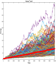
(a) ${\rm Energy-preserving}$

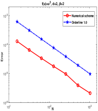
(b) ${\rm Spatial\;error}$

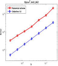
(c) ${\rm Temporal\;error}$

Figure 1: Energy-preserving property and strong convergence order in space and time for the full discrete numerical method (16) applied to stochastic wave equation (27).

Fig. 1(a) presents the evolution of discrete energy using the proposed methods in Section 4, where the red line represents the discrete averaged energy along 500 trajectories. From Theorem 4.1, we noted that, the averaged energy evolution law $\mathbb{E}(V_{1}(u_{m}^{N},v_{m}^{N}))$ follows a linear evolution with growth rate $\frac{1}{2}{\rm Tr}((P_{N}\mathbf{Q}^{\frac{1}{2}})(P_{N}\mathbf{Q}^{\frac{1}{2}})^{*})$. It can be observed from Fig. 1(a) that the discrete averaged energy obeys nearly linear growth over 500 trajectories, which coincides with the theoretical analysis.

Now let us start with tests on the convergence rates. First of all, we consider the spatial convergence rate of the numerical method (16). The middle figure in Fig. 1 displays the spatial approximation errors $\sup\limits_{0\leq t\leq T}\|X_{N}(t)-X(t)\|_{L^{p}(\Omega;\mathbb{H})}$ against $N$ on a log-log scale with $N=2^{s},~{}s=4,5,\cdots,9$. It can be observed that the slope is closed to $1$ which is consistent with our previous theoretical result (see Proposition 3.4) on the spatial convergence order. Note that for the temporal discretization we used here the proposed method (16) at a sufficiently small time step-size $h=2^{-10}$. In addition, $N=2^{11}$ is used to simulate the exact solution.

To investigate the strong convergence order in temporal direction of (16) by using various step-sizes $h=2^{-r},~{}r=2,3,\cdots,7$, we now fix $N=100$. Again, the “exact” solution is approximated by the method (16) with a very small time step-size $h=2^{-12}$. The right figure in Fig. 1 presents the strong approximation errors of the proposed method (16) in temporal direction. It can be seen that this numerical performance coincides with the theoretical assertion (see Proposition 4.3).

Acknowledgment. The authors are very grateful to the referees for their valuable comments and suggestions on the improvement of the present paper.

6 Appendix

Existence and uniqueness of numerical solution of (16). To prove the well-posedness of the numerical scheme, it only needs to show that the existence and uniqueness of numerical solution of the scheme at the step $m+1$. Assume that $d\leq 2,$ $\|\mathbf{Q}^{\frac{1}{2}}\|_{\mathcal{L}_{2}(L^{2})}<\infty,$ $h_{0}>0$ is sufficient small, temporal step size $h<h_{0}$, and that $(u_{m}^{N},v_{m}^{N})^{\top}\in\mathbb{H}^{1}$ is $\mathcal{F}_{t_{m}}$-measurable and $\mathbb{E}\Big{[}\exp({V_{1}(u_{m}^{N},v_{m}^{N})}{e^{-\alpha t_{m}}})\Big{]}\leq C$ for some $\alpha(Q,T,u_{0},v_{0},d)\geq 1$ and $C(Q,T,u_{0},v_{0},d)>0$. The proof is similar to that of [24, Lemma 8.1] by making use of the structure of the drift coefficient $f$ and the fact that (LABEL:mod;swe) is a separable system.

Since the last equation in (16) has an explicit analytical solution, it suffices to show the existence of a unique solution for the first two equations in (16), that is,

$$u^{N}_{m+1}= u^{N}_{m}+h\bar{v}^{N}_{m+\frac{1}{2}},$$ (28)

$$\bar{v}^{N}_{m+1}= v^{N}_{m}+h\Lambda_{N}u^{N}_{m+\frac{1}{2}}-hP_{N}\left(\int_{0}^{1}f(u^{N}_{m}+\theta(u^{N}_{m+1}-u^{N}_{m}))d\theta\right).$$

Finding the solution of the above system is equivalent to the solvability of finding $\widetilde{v}$ such that

$$\widetilde{v}-v^{N}_{m}-\frac{1}{2}h\Lambda_{N}(u^{N}_{m}+\frac{1}{2}h\widetilde{v})+\frac{1}{2}hP_{N}\left(\int_{0}^{1}f(u^{N}_{m}+\theta h\widetilde{v})d\theta\right)=0.$$

Choosing $\widetilde{F}(x,y)>0$ as the anti-derivative of $\frac{1}{2}h\int_{0}^{1}f(x+\theta hy)d\theta$ for fixed $x$, then it suffices to find $v^{*}$ which minimizes

$$\frac{1}{2}\|\widetilde{v}-v^{N}_{m}\|_{L^{2}}^{2}+\frac{1}{2}\|u^{N}_{m}+\frac{1}{2}h\widetilde{v}\|_{\mathbb{\dot{\mathbb{H}}}^{1}}^{2}+\int_{\mathcal{O}}\widetilde{F}(u^{N}_{m},\widetilde{v})dx.$$

The existence of the minimizer is guaranteed by the fact that $f(\cdot)$ is smooth and its anti-derivative is bounded below. Furthermore, the uniqueness can be obtained by using the fact $f(u)=c_{3}u^{3}+\cdots+c_{1}u+c_{0}$ is a polynomial with $c_{3}>0$. It implies that there exists $C(c_{3},c_{2},c_{1},c_{0})>0$ such that $(f(x)-f(y))\cdot(x-y)\geq-C\|x-y\|^{2}.$

Assume that we have two different numerical solutions $(\widetilde{u}_{1},\widetilde{v}_{1})$ and $(\widetilde{u}_{2},\widetilde{v}_{2})$ in $P_{N}(\mathbb{H})$ of (16) with the same initial condition $(u_{m}^{N},v_{m}^{N})$. Then

$$\widetilde{v}_{i}-\frac{1}{2}h\Lambda_{N}(u_{m}^{N}+\frac{h}{2}\widetilde{v}_{i})+P_{N}\left(\frac{\partial}{\partial y}\widetilde{F}(u^{N}_{m},\widetilde{v}_{i})\right)=v_{m}^{N},\;i=1,2.$$

Using $c_{3}>0$ and the Poincaré inequality, we have that

$$0\geq(1+\lambda_{1}\frac{h^{2}}{4}-C^{\prime}h^{2})\|\widetilde{v}_{1}-\widetilde{v}_{2}\|_{L^{2}}^{2}$$

for some constant $C^{\prime}(c_{3},c_{2},c_{1},c_{0}).$ By taking $h_{0}$ small enough such that $1+\lambda_{1}\frac{h_{0}^{2}}{4}>C^{\prime}h_{0}^{2}$, the uniqueness of the numerical solution of (16) is obtained.

Strong approximate error of the fixed point iteration. Assume that $(u_{m}^{N},v_{m}^{N})$ is the numerical solution at time step $m.$ The first fixed point iteration reads

$$\begin{split}&u^{N,k+1}=u^{N}_{m}+h\bar{v}^{N,k+\frac{1}{2}},\\ &\bar{v}^{N,k+1}=v^{N}_{m}+h\Lambda_{N}u^{N,k+\frac{1}{2}}-hP_{N}\Big{(}\frac{1}{2}((u^{N,k})^{2}+(u^{N}_{m})^{2})-1\Big{)}u^{N,k+\frac{1}{2}},\\ &u^{N,0}=u^{N}_{m},\quad v^{N,0}=v^{N}_{m},\end{split}$$ (29)

where $u^{N,k+\frac{1}{2}}=\frac{1}{2}(u^{N,k+1}+u^{N}_{m}),$ $\bar{v}^{N,k+\frac{1}{2}}=\frac{1}{2}(\bar{v}^{N,k+1}+v^{N}_{m}).$ The second one takes the form of

$$\begin{split}u^{N,k+1}=&u^{N}_{m}+h\bar{v}^{N,k+\frac{1}{2}},\\ \bar{v}^{N,k+1}=&v^{N}_{m}+h\Lambda_{N}u^{N,k+\frac{1}{2}}\\ &-h\mathbb{I}_{\{\|u^{N,k}\|_{\dot{\mathbb{H}}^{1}}+\|u^{N}_{m}\|_{\dot{\mathbb{H}}^{1}}\leq\frac{1}{\epsilon}\}}P_{N}\Big{(}\frac{1}{2}\Big{(}(u^{N,k})^{2}+(u^{N}_{m})^{2}\Big{)}-1\Big{)}u^{N,k+\frac{1}{2}}\end{split}$$ (30)

with $u^{N,0}=u^{N}_{m},v^{N,0}=v^{N}_{m}$ and a sufficiently small parameter $\epsilon>0$. Under the assumption on the well-posedness of numerical solution in Appendix, we obtain that (LABEL:iteration1) satisfies for small $h\in(0,h_{0})$ with $h^{2}\lambda_{N}^{\frac{d}{3}}=O(1),$

$$\mathbb{E}\Big{[}\|u^{N,k}-u^{*}\|_{L^{2}}^{2}\Big{]}+\mathbb{E}\Big{[}\|v^{N,k}-v^{*}\|_{\dot{\mathbb{H}}^{-1}}^{2}\Big{]}$$

$$\leq Ch^{2}(1+h^{2}\lambda_{N}^{\frac{d}{3}})^{2}\left((\frac{1}{2})^{k+1}+\exp(-\eta h^{-1}\min(h^{-2}\lambda_{N}^{-\frac{d}{3}},1))\right),$$ (31)

and (30) satisfies for small $h\in(0,h_{0})$ with $\frac{h}{\epsilon^{4}}=O(1),$

$$\mathbb{E}\Big{[}\|u^{*}-u^{N,k+1}\|_{L^{2}}^{2}\Big{]}+\mathbb{E}\Big{[}\|v^{N,k}-v^{*}\|_{\dot{\mathbb{H}}^{-1}}^{2}\Big{]}$$

$$\leq C\max(h^{2},\epsilon^{8})\Big{(}(\frac{1}{2})^{k+1}+\exp(-\eta\frac{1}{\epsilon^{2}})\Big{)},$$ (32)

where $(u^{*},v^{*})$ is the fixed point of (28), i.e., $(u^{*},v^{*})=(u_{m+1}^{N},\bar{v}_{m+1}^{N})$, and $\eta,C>0$ depend on $T,Q,d,u^{N}_{m},v^{N}_{m}.$ Here $h_{0}$ is the upper bound of the step-size such that the fixed point of (28) exists uniquely.

$\bullet$ Analysis of fixed point iterations of (LABEL:iteration1)

Since the stochastic subsystem in (16) possesses a unique explicit solution, it suffices to construct iterations to approximate the fixed point of (28). Thanks to the polynomial assumption on $f$, we have that

$$\int_{0}^{1}f(u^{N}_{m}+\theta(u^{N}_{m+1}-u^{N}_{m}))d\theta =\frac{1}{4}\frac{(u^{N}_{m+1})^{4}-(u^{N}_{m})^{4}}{u^{N}_{m+1}-u^{N}_{m}}-\frac{1}{2}\frac{(u^{N}_{m+1})^{2}-(u^{N}_{m})^{2}}{u^{N}_{m+1}-u^{N}_{m}}$$

$$=\Big{(}\frac{1}{2}((u^{N}_{m+1})^{2}+(u^{N}_{m})^{2})-1\Big{)}u^{N}_{m+\frac{1}{2}},$$

which yields

$$\begin{split}\frac{u^{N}_{m}+u^{*}}{2}=&u^{N}_{m}+\frac{1}{2}hv^{N}_{m}+\frac{1}{4}h^{2}\Lambda_{N}\left(\frac{u^{N}_{m}+u^{*}}{2}\right)\\ &-\frac{1}{4}h^{2}P_{N}\Big{(}\frac{1}{2}((u^{*})^{2}+(u^{N}_{m})^{2})-1\Big{)}\left(\frac{u^{N}_{m}+u^{*}}{2}\right).\end{split}$$ (33)

Moreover, we rewrite (LABEL:iteration1) as

$$\begin{split}u^{N,k+\frac{1}{2}}=&u^{N}_{m}+\frac{1}{2}hv^{N}_{m}+\frac{1}{4}h^{2}\Lambda_{N}u^{N,k+\frac{1}{2}}\\ &-\frac{1}{4}h^{2}P_{N}\Big{(}\frac{1}{2}((u^{N,k})^{2}+(u^{N}_{m})^{2})-1\Big{)}u^{N,k+\frac{1}{2}}.\end{split}$$ (34)

To prove (6), we estimate

$$\mathbb{E}\Big{[}\|u^{N,k+\frac{1}{2}}-\frac{1}{2}(u^{*}+u^{N}_{m})\|_{L^{2}}^{2}\Big{]}+\mathbb{E}\Big{[}\|{\bar{v}}^{N,k+\frac{1}{2}}-\frac{1}{2}(v^{*}+v^{N}_{m})\|_{\dot{\mathbb{H}}^{-1}}^{2}\Big{]}.$$

Let us take $\mathbb{E}\Big{[}\|u^{N,k+\frac{1}{2}}-\frac{1}{2}(u^{*}+u^{N}_{m})\|_{L^{2}}^{2}\Big{]}$ as an example to illustrate the detailed steps and estimates, since the estimate of $\mathbb{E}\Big{[}\|{\bar{v}}^{N,k+\frac{1}{2}}-\frac{1}{2}(v^{*}+v^{N}_{m})\|_{\dot{\mathbb{H}}^{-1}}^{2}\Big{]}$ is analogous.

First, we claim that the a priori estimate of $u^{N,k+\frac{1}{2}}$ could be bounded by the estimates of $u^{N}_{m}$ and $v^{N}_{m}$. To this end, we take $L^{2}$-inner product with $u^{N,k+\frac{1}{2}}$ on (34) and use the integration by part formula and Young’s inequality, then

$$\|u^{N,k+\frac{1}{2}}\|_{L^{2}}^{2}\leq \langle u^{N}_{m}+\frac{1}{2}hv^{N}_{m},u^{N,k+\frac{1}{2}}\rangle_{L^{2}}+\frac{1}{4}h^{2}\langle\Lambda_{N}u^{N,k+\frac{1}{2}},u^{N,k+\frac{1}{2}}\rangle_{L^{2}}$$

$$-\frac{1}{4}h^{2}\langle\Big{(}\frac{1}{2}((u^{N,k})^{2}+(u^{N}_{m})^{2})-1\Big{)}u^{N,k+\frac{1}{2}},u^{N,k+\frac{1}{2}}\rangle_{L^{2}}$$

$$\leq \frac{1}{2}\|u^{N}_{m}+\frac{1}{2}hv^{N}_{m}\|_{L^{2}}^{2}+\|u^{N,k+\frac{1}{2}}\|_{L^{2}}^{2}(\frac{1}{2}+\frac{1}{4}h^{2})-\frac{1}{4}h^{2}\|\nabla u^{N,k+\frac{1}{2}}\|_{L^{2}}^{2}.$$

Then since $\lambda_{1}\geq 1,$ by the Poincaré inequality, we have that

$$\frac{1}{2}\|u^{N,k+\frac{1}{2}}\|_{L^{2}}^{2} \leq\frac{1}{2}\|u^{N}_{m}+\frac{1}{2}hv^{N}_{m}\|_{L^{2}}^{2}.$$

Similarly, one could get that for $q\in\mathbb{N}^{+},$

$$\|u^{N,k+\frac{1}{2}}\|_{L^{2q}}^{2q} \leq C_{q}\|u^{N}_{m}+\frac{1}{2}hv^{N}_{m}\|_{L^{2q}}^{2q}.$$ (35)

By subtracting the corresponding equation (33) of $\frac{u_{m}^{N}+u^{*}}{2}$ from (34), we achieve that

$$u^{N,k+\frac{1}{2}}-\frac{u_{m}^{N}+u^{*}}{2}= \frac{1}{4}h^{2}\Lambda_{N}(u^{N,k+\frac{1}{2}}-\frac{u_{m}^{N}+u^{*}}{2})$$

$$-\frac{1}{4}h^{2}P_{N}\Big{(}\frac{1}{2}((u^{N,k})^{2}+(u^{N}_{m})^{2})-1\Big{)}(u^{N,k+\frac{1}{2}}-\frac{u_{m}^{N}+u^{*}}{2})$$

$$-\frac{1}{4}h^{2}P_{N}\Big{(}\frac{1}{2}(u^{N,k})^{2}-\frac{1}{2}(u^{*})^{2}\Big{)}\frac{u_{m}^{N}+u^{*}}{2}.$$

Then multiplying $u^{N,k+\frac{1}{2}}-\frac{u_{m}^{N}+u^{*}}{2}$ on both sides of the above equation, using integration by parts, the Sobolev embedding theorem $L^{\frac{6}{5}}\hookrightarrow\dot{\mathbb{H}}^{-\frac{d}{3}}$ and Young’s inequality, we have that for $k\geq 1,$

$$\|u^{N,k+\frac{1}{2}}-\frac{u_{m}^{N}+u^{*}}{2}\|_{L^{2}}^{2}$$

$$\leq -\frac{1}{4}h^{2}\left\|(-\Lambda)^{\frac{1}{2}}\left(u^{N,k+\frac{1}{2}}-\frac{u_{m}^{N}+u^{*}}{2}\right)\right\|_{L^{2}}^{2}+\frac{1}{4}h^{2}\|u^{N,k+\frac{1}{2}}-\frac{u_{m}^{N}+u^{*}}{2}\|_{L^{2}}^{2}$$

$$-\frac{1}{4}h^{2}P_{N}\left\langle(-\Lambda)^{-\frac{1}{2}}\left(\Big{(}\frac{1}{2}(u^{N,k})^{2}-\frac{1}{2}(u^{*})^{2}\Big{)}\frac{u_{m}^{N}+u^{*}}{2}\right),(-\Lambda)^{\frac{1}{2}}\big{(}u^{N,k+\frac{1}{2}}-\frac{u_{m}^{N}+u^{*}}{2}\big{)}\right\rangle_{L^{2}}$$

$$\leq \frac{1}{4}h^{2}\|u^{N,k+\frac{1}{2}}-\frac{u_{m}^{N}+u^{*}}{2}\|_{L^{2}}^{2}$$

$$+h^{2}C\Big{(}\|u^{N,k}\|_{L^{6}}^{4}+\|u_{m}^{N}\|_{L^{6}}^{4}+\|u^{*}\|_{L^{6}}^{4}\Big{)}\left\|u^{N,k-\frac{1}{2}}-\frac{u_{m}^{N}+u^{*}}{2}\right\|_{L^{2}}^{2},$$

where $C$ depends on the coefficient of Sobolev embedding inequality $L^{\frac{6}{5}}\hookrightarrow\dot{\mathbb{H}}^{-\frac{d}{3}}$. This implies that

$$\|u^{N,k+1}-u^{*}\|_{L^{2}}^{2}$$

$$\leq \frac{Ch^{2}}{1-\frac{1}{4}h^{2}}\Big{(}\|u^{N,k}\|_{L^{6}}^{4}+\|u_{m}^{N}\|_{L^{6}}^{4}+\|u^{*}\|_{L^{6}}^{4}\Big{)}\|u^{N,k}-u^{*}\|_{L^{2}}^{2}$$ (36)

$$\leq (\frac{Ch^{2}}{1-\frac{1}{4}h^{2}})^{k+1}\prod_{j=0}^{k}\Big{(}\|u^{N,j}\|_{L^{6}}^{4}+\|u_{m}^{N}\|_{L^{6}}^{4}+\|u^{*}\|_{L^{6}}^{4}\Big{)}\|u^{N,0}-u^{*}\|_{L^{2}}^{2}.$$

One could use the Sobolev embedding theorem $\dot{\mathbb{H}}^{\frac{d}{3}}\hookrightarrow L^{6}$, the inverse inequality in $U^{N}$ and (35), and get for small $h\in(0,1)$,

$$\|u^{N,k+1}-u^{*}\|_{L^{2}}^{2}$$

$$\leq (\frac{C^{\prime}h^{2}}{1-\frac{1}{4}h^{2}})^{k+1}\prod_{j=0}^{k}\Big{(}\lambda_{N}^{\frac{2d}{3}}h^{4}\|v^{N}_{m}\|_{L^{2}}^{4}+\|u^{N}_{m}\|_{L^{6}}^{4}+\|u^{*}\|_{L^{6}}^{4}\Big{)}\|u^{N,0}-u^{*}\|_{L^{2}}^{2},$$

where $C^{\prime}=C\max(1,C_{sob}^{4}),$ where $C_{sob}$ is the coefficient of the Sobolev embedding $\dot{\mathbb{H}}^{\frac{d}{3}}\hookrightarrow L^{6}.$ Furthermore, on the subset

$$\Omega_{h}:=\Big{\{}\omega\in\Omega\Big{|}\lambda_{N}^{\frac{2d}{3}}h^{4}\|v^{N}_{m}\|_{L^{2}}^{4}+\|u^{N}_{m}\|_{L^{6}}^{4}+\|u^{*}\|_{L^{6}}^{4}\leq\frac{1-\frac{1}{4}h^{2}}{2C^{\prime}h^{2}}\Big{\}},$$

it holds that for

$$\mathbb{E}\Big{[}\mathbb{I}_{\Omega_{h}}\|u^{N,k+1}-u^{*}\|_{L^{2}}^{2}\Big{]} \leq\left(\frac{1}{2}\right)^{k+1}\mathbb{E}\Big{[}\|u^{N,0}-u^{*}\|_{L^{2}}^{2}\Big{]}$$

$$\leq\left(\frac{1}{2}\right)^{k+1}h^{2}\mathbb{E}\Big{[}\|\frac{v_{m}^{N}+v^{*}}{2}\|_{L^{2}}^{2}\Big{]}$$

$$\leq C(Q,T,u_{m}^{N},v_{m}^{N},d)h^{2}\left(\frac{1}{2}\right)^{k+1}.$$

Notice that the fixed point of (28) in the revised paper possesses the energy preserving property $V_{1}(u^{*},v^{*})=V_{1}(u^{N}_{m},v^{N}_{m}).$ The first equality of (36), together with (35), the moment boundedness of $V_{1}(u^{N}_{m},v^{N}_{m})$ and $V_{1}(u^{*},v^{*})$, and the inverse Sobolev inequality, yield that for $p\geq 1$,

$$\quad\mathbb{E}\Big{[}\|u^{N,k+1}-u^{*}\|_{L^{2}}^{2p}\Big{]}$$ (37)

$$\leq(\frac{Ch^{2}}{1-\frac{1}{4}h^{2}})^{p}\Big{(}\mathbb{E}\Big{[}\Big{(}\|u^{N,k}\|_{L^{6}}^{8p}+\|u_{m}^{N}\|_{L^{6}}^{8p}+\|u^{*}\|_{L^{6}}^{8p}\Big{)}\Big{]}\Big{)}^{\frac{1}{2}}\Big{(}\mathbb{E}\Big{[}\|u^{N,k-\frac{1}{2}}-\frac{u_{m}^{N}+u^{*}}{2}\|_{L^{2}}^{4p}\Big{]}\Big{)}^{\frac{1}{2}}$$

$$\leq(\frac{Ch^{2}}{1-\frac{1}{4}h^{2}})^{p}\Big{(}1+\Big{(}\mathbb{E}\Big{[}\|u^{N}_{m}\|_{L^{6}}^{8p}\Big{]}\Big{)}^{\frac{1}{2}}+(h\lambda_{N}^{\frac{d}{6}})^{4p}\Big{(}\mathbb{E}\Big{[}\|v^{N}_{m}\|_{L^{2}}^{8p}\Big{]}\Big{)}^{\frac{1}{2}}\Big{)}$$

$$\quad\times\Big{(}\mathbb{E}\Big{[}\|u^{N,k}\|_{L^{2}}^{4p}+\|u_{m}^{N}\|_{L^{2}}^{4p}+\|u^{*}\|_{L^{2}}^{4p}\Big{]}\Big{)}^{\frac{1}{2}}$$

$$\leq C(T,Q,p,d,u^{N}_{m},v^{N}_{m})(h(1+h^{2}\lambda_{N}^{\frac{d}{3}}))^{2p},$$

where $C$ differs from line to line up to a constant depending on $p,$ and $C(T,Q,p,d,u^{N}_{m},v^{N}_{m})<\infty$ due to $\eqref{L6-est}$ and the energy preserving property of the fixed point. On the set $\Omega_{h}^{c}$, by (37) and the Chebshev inequality, we have that there exists $C>0$ depending on $T,Q,u^{N}_{m},v^{N}_{m},d$ such that

$$\mathbb{E}\Big{[}\mathbb{I}_{\Omega_{h}^{c}}\|u^{N,k+1}-u^{*}\|_{L^{2}}^{2}\Big{]}$$

$$\leq \Big{(}\mathbb{P}(\lambda_{N}^{\frac{2d}{3}}h^{4}\|v^{N}_{m}\|_{L^{2}}^{4}+\|u^{N}_{m}\|_{L^{6}}^{4}+\|u^{*}\|_{L^{6}}^{4}\geq\frac{1-\frac{1}{4}h^{2}}{2C^{\prime}h^{2}})\Big{)}^{\frac{1}{2}}$$

$$\quad\times\sqrt{\mathbb{E}\Big{[}\|u^{N,k+1}-u^{*}\|_{L^{2}}^{4}\Big{]}}$$

$$\leq Ch^{2}(1+h^{2}\lambda_{N}^{\frac{d}{3}})^{2}\Big{(}\mathbb{P}(\lambda_{N}^{\frac{2d}{3}}h^{4}\|v^{N}_{m}\|_{L^{2}}^{4}+\|u^{N}_{m}\|_{L^{6}}^{4}+\|u^{*}\|_{L^{6}}^{4}\geq\frac{1-\frac{1}{4}h^{2}}{2C^{\prime}h^{2}})\Big{)}^{\frac{1}{2}}.$$

Now applying the Gaussian type tail estimates for $(u_{m}^{N},v_{m}^{N})$ and $(u^{*},v^{*})$ which possess some exponential integrability (see e.g. the proof of [13, Corollary 4.1]), and using the Sobolev embedding theorem, the assumption

$$\mathbb{E}\Big{[}\exp({V_{1}(u_{m}^{N},v_{m}^{N})}{e^{-\alpha t_{m}}})\Big{]}<\infty$$

in Appendix, as well as the definition of $V_{1}$, we get that

$$\mathbb{P}\Big{(}\lambda_{N}^{\frac{2d}{3}}h^{4}\|v^{N}_{m}\|_{L^{2}}^{4}+\|u^{N}_{m}\|_{L^{6}}^{4}+\|u^{*}\|_{L^{6}}^{4}\geq\frac{1-\frac{1}{4}h^{2}}{2C^{\prime}h^{2}}\Big{)}$$

$$\leq \mathbb{P}\Big{(}\|v^{N}_{m}\|_{L^{2}}\geq h^{-1}\lambda_{N}^{-\frac{d}{6}}(\frac{1}{3}\frac{1-\frac{1}{4}h^{2}}{2C^{\prime}h^{2}})^{\frac{1}{4}}\Big{)}+\mathbb{P}\Big{(}\|u^{N}_{m}\|_{\dot{\mathbb{H}}^{1}}\geq(\frac{C_{sob}^{4}}{3}\frac{1-\frac{1}{4}h^{2}}{2C^{\prime}h^{2}})^{\frac{1}{4}}\Big{)}$$

$$+\mathbb{P}\Big{(}\|u^{*}\|_{\dot{\mathbb{H}}^{1}}\geq(\frac{C_{sob}^{4}}{3}\frac{1-\frac{1}{4}h^{2}}{2C^{\prime}h^{2}})^{\frac{1}{4}}\Big{)}$$

$$\leq C_{11}\exp(-\eta_{1}(h^{-2}\lambda_{N}^{-\frac{d}{3}}(\frac{1}{3}\frac{1-\frac{1}{4}h^{2}}{2C^{\prime}h^{2}})^{\frac{1}{2}}))+C_{12}\exp(-\eta_{2}(\frac{C_{sob}^{4}}{3}\frac{1-\frac{1}{4}h^{2}}{2C^{\prime}h^{2}})^{\frac{1}{2}})$$

$$+C_{13}\exp(-\eta_{3}(\frac{C_{sob}^{4}}{3}\frac{1-\frac{1}{4}h^{2}}{2C^{\prime}h^{2}})^{\frac{1}{2}}),$$

where $C_{sob}$ is the coefficient of Sobolev embedding inequality from $\dot{\mathbb{H}}^{1}$ to $L^{6},$

$$C_{11} =\mathbb{E}[\exp(\frac{1}{2}\|v_{m}^{N}\|_{L^{2}}^{2}e^{-\alpha{t_{m}}})],C_{12}=C_{13}=\mathbb{E}[\exp(\frac{1}{2}\|u_{m}^{N}\|_{{\dot{\mathbb{H}}^{1}}}^{2}e^{-\alpha{t_{m}}})],$$

$$\eta_{1} =\eta_{2}=\eta_{3}=\frac{1}{2}e^{-\alpha{t_{m}}}.$$

Therefore, we have that

$$\quad\mathbb{E}\Big{[}\mathbb{I}_{\Omega_{h}^{c}}\|u^{N,k+1}-u^{*}\|_{L^{2}}^{2}\Big{]}$$

$$\leq Ch^{2}(1+h^{2}\lambda_{N}^{\frac{d}{3}})^{2}\Big{(}\mathbb{P}(\lambda_{N}^{\frac{2d}{3}}h^{4}\|v^{N}_{m}\|_{L^{2}}^{4}+\|u^{N}_{m}\|_{L^{6}}^{4}+\|u^{*}\|_{L^{6}}^{4}\geq\frac{1-\frac{1}{4}h^{2}}{2C^{\prime}h^{2}})\Big{)}^{\frac{1}{2}}$$

$$\leq Ch^{2}(1+h^{2}\lambda_{N}^{\frac{d}{3}})^{2}(C_{11}^{\frac{1}{2}}+C_{12}^{\frac{1}{2}}+C_{13}^{\frac{1}{2}})\times$$

$$\max(\exp(-\eta_{1}(h^{-2}\lambda_{N}^{-\frac{d}{3}}(\frac{1}{3}\frac{1-\frac{1}{4}h^{2}}{2C^{\prime}h^{2}})^{\frac{1}{2}})),\exp(-\eta_{3}(\frac{C_{sob}^{4}}{3}\frac{1-\frac{1}{4}h^{2}}{2C^{\prime}h^{2}})^{\frac{1}{2}})).$$

Choosing $h\in(0,1)$ small enough, we conclude that there exist $\eta,C>0$ depending on $Q,T,u_{m}^{N},v_{m}^{N},d$ such that

$$\mathbb{E}\Big{[}\mathbb{I}_{\Omega_{h}^{c}}\|u^{N,k+1}-u^{*}\|_{L^{2}}^{2}\Big{]}$$

$$\leq Ch^{2}(1+h^{2}\lambda_{N}^{\frac{d}{3}})^{2}\exp(-\eta h^{-1}\min(h^{-2}\lambda_{N}^{-\frac{d}{3}},1)).$$

Combining the above two estimates on $\Omega_{h}$ and $\Omega_{h}^{c}$, we complete the proof.

$\bullet$Analysis of fixed point iterations of (30)

Using the mild form of (30) and the unitary property of $\mathbb{B}^{-1}(h)\mathbb{A}(h)$ in Lemma 4.1 and the expression of $\mathbb{B}^{-1}(h)$, we have that for $k\in\mathbb{N}^{+}$,

$$\sqrt{\|u^{N,k+1}\|_{\dot{\mathbb{H}}^{1}}^{2}+\|\bar{v}^{N,k+1}\|_{L^{2}}^{2}}$$

$$\leq \sqrt{\|u^{N}_{m}\|_{\dot{\mathbb{H}}^{1}}^{2}+\|v^{N}_{m}\|_{L^{2}}^{2}}+hC\Big{(}\|u^{N,k+\frac{1}{2}}\|_{L^{2}}+\|u^{N,k+\frac{1}{2}}\|_{L^{6}}(\|u^{N,k}\|_{L^{6}}^{2}+\|u^{N}_{m}\|_{L^{6}}^{2})\Big{)}$$

$$\times\mathbb{I}_{\{\|u^{N,k}\|_{\dot{\mathbb{H}}^{1}}+\|u^{N}_{m}\|_{\dot{\mathbb{H}}^{1}}\leq\frac{1}{\epsilon}\}}$$

$$\leq \sqrt{\|u^{N}_{m}\|_{\dot{\mathbb{H}}^{1}}^{2}+\|v^{N}_{m}\|_{L^{2}}^{2}}+hC(1+\frac{1}{\epsilon^{2}})\sqrt{\|u^{N,k+1}\|_{\dot{\mathbb{H}}^{1}}^{2}+\|\bar{v}^{N,k+1}\|_{L^{2}}^{2}}+Ch(\frac{1}{\epsilon}+\frac{1}{\epsilon^{3}}).$$

This implies that if $hC(1+\frac{1}{\epsilon^{2}})\leq c<1,$ then there exists $C^{\prime}>0$ such that

$$\sqrt{\|u^{N,k+1}\|_{\dot{\mathbb{H}}^{1}}^{2}+\|\bar{v}^{N,k+1}\|_{L^{2}}^{2}}$$ (38)

$$\leq (1+C^{\prime}h(1+\frac{1}{\epsilon^{2}}))\sqrt{\|u^{N}_{m}\|_{\dot{\mathbb{H}}^{1}}^{2}+\|v^{N}_{m}\|_{L^{2}}^{2}}+(1+C^{\prime}h(1+\frac{1}{\epsilon^{2}}))Ch(\frac{1}{\epsilon}+\frac{1}{\epsilon^{3}}).$$

Let us consider the difference between $\frac{u^{*}+u^{N}_{m}}{2}$ and $u^{N,k+\frac{1}{2}}$. The estimate with respect to $v^{*}$ and $\bar{v}^{N,k+1}$ is similar. By substituting the equation of $\bar{v}^{N,k+1}$ into the equation of $u^{N,k+1}$, we have that

$$u^{N,k+\frac{1}{2}}= u^{N}_{m}+\frac{h}{2}v^{N}_{m}+\frac{h^{2}}{4}\Lambda_{N}u^{N,k+\frac{1}{2}}-\frac{h^{2}}{4}P_{N}\Big{(}\frac{1}{2}\Big{(}(u^{N,k})^{2}+(u^{N}_{m})^{2}\Big{)}-1\Big{)}u^{N,k+\frac{1}{2}}$$

$$\times\mathbb{I}_{\{\|u^{N,k}\|_{\dot{\mathbb{H}}^{1}}+\|u^{N}_{m}\|_{\dot{\mathbb{H}}^{1}}\leq\frac{1}{\epsilon}\}}.$$

By subtracting the above equation from the equation of $\frac{u^{*}+u^{N}_{m}}{2}$, taking $L^{2}$-inner product with $\frac{u^{*}+u^{N}_{m}}{2}-u^{N,k+\frac{1}{2}}$ and using Young’s inequality, we obtain

$$\|\frac{u^{*}+u^{N}_{m}}{2}-u^{N,k+\frac{1}{2}}\|_{L^{2}}^{2}$$

$$\leq -\frac{h^{2}}{8}\|\nabla(\frac{u^{*}+u^{N}_{m}}{2}-u^{N,k+\frac{1}{2}})\|_{L^{2}}^{2}+\frac{h^{2}}{4}\|\frac{u^{*}+u^{N}_{m}}{2}-u^{N,k+\frac{1}{2}}\|_{L^{2}}^{2}$$

$$+\frac{h^{2}}{8}\|(u^{N,k})^{2}u^{N,k+\frac{1}{2}}-(u^{*})^{2}\frac{u^{*}+u^{N}_{m}}{2}\|_{\dot{\mathbb{H}}^{-1}}^{2}\mathbb{I}_{\{\|u^{N,k}\|_{\dot{\mathbb{H}}^{1}}+\|u^{N}_{m}\|_{\dot{\mathbb{H}}^{1}}\leq\frac{1}{\epsilon}\}}$$

$$-\frac{h^{2}}{4}\langle(\frac{1}{2}((u^{*})^{2}+(u^{N}_{m})^{2})-1)\frac{u^{*}+u^{N}_{m}}{2},\frac{u^{*}+u^{N}_{m}}{2}-u^{N,k+\frac{1}{2}}\rangle_{L^{2}}\mathbb{I}_{\{\|u^{N,k}\|_{\dot{\mathbb{H}}^{1}}+\|u^{N}_{m}\|_{\dot{\mathbb{H}}^{1}}>\frac{1}{\epsilon}\}}$$

$$\leq \frac{h^{2}}{4}\|\frac{u^{*}+u^{N}_{m}}{2}-u^{N,k+\frac{1}{2}}\|_{L^{2}}^{2}$$

$$+\frac{h^{2}}{8}\|(u^{N,k})^{2}u^{N,k+\frac{1}{2}}-(u^{*})^{2}\frac{u^{*}+u^{N}_{m}}{2}\|_{\mathbb{H}^{-1}}^{2}\mathbb{I}_{\{\|u^{N,k}\|_{\dot{\mathbb{H}}^{1}}+\|u^{N}_{m}\|_{\dot{\mathbb{H}}^{1}}\leq\frac{1}{\epsilon}\}}$$

$$+\frac{h^{2}}{8}\|(\frac{1}{2}((u^{*})^{2}+(u^{N}_{m})^{2})-1)\frac{u^{*}+u^{N}_{m}}{2}\|^{2}_{\dot{\mathbb{H}}^{-1}}\mathbb{I}_{\{\|u^{N,k}\|_{\dot{\mathbb{H}}^{1}}+\|u^{N}_{m}\|_{\dot{\mathbb{H}}^{1}}>\frac{1}{\epsilon}\}}.$$

By applying the the Sobolev embedding $L^{\frac{6}{5}}\hookrightarrow\dot{\mathbb{H}}^{-\frac{d}{3}}$ and Young’s inequality, we further have that for small $h\in(0,1),$

$$\|\frac{u^{*}+u^{N}_{m}}{2}-u^{N,k+\frac{1}{2}}\|_{L^{2}}^{2}$$

$$\leq C{h^{2}}\Big{(}\|u^{N,k}-u^{*}\|_{L^{2}}^{2}(\|u^{N,k}\|_{L^{6}}^{2}+\|u^{*}\|_{L^{6}}^{2})(\|u^{*}\|_{L^{6}}^{2}+\|u^{N}_{m}\|_{L^{6}}^{2})$$

$$+\|u^{N,k}\|_{L^{6}}^{4}\|u^{N,k+\frac{1}{2}}-\frac{u^{*}+u^{N}_{m}}{2}\|_{L^{2}}^{2}\Big{)}\mathbb{I}_{\{\|u^{N,k}\|_{\dot{\mathbb{H}}^{1}}+\|u^{N}_{m}\|_{\dot{\mathbb{H}}^{1}}\leq\frac{1}{\epsilon}\}}$$

$$+C{h^{2}}\Big{(}\|u^{*}\|_{L^{2}}^{2}+\|u^{N}_{m}\|_{L^{2}}^{2}+\|u^{*}\|_{L^{6}}^{6}+\|u^{N}_{m}\|_{L^{6}}^{6}\Big{)}\mathbb{I}_{\{\|u^{N,k}\|_{\dot{\mathbb{H}}^{1}}+\|u^{N}_{m}\|_{\dot{\mathbb{H}}^{1}}>\frac{1}{\epsilon}\}}.$$

Notice that the energy preservation of $(u^{*},v^{*})$ leads to

$$\frac{1}{2}\|u^{*}\|_{\dot{\mathbb{H}}^{1}}^{2}+\frac{1}{2}\|v^{*}\|_{L^{2}}^{2}+\frac{1}{4}\|u^{*}\|_{L^{4}}^{4} \leq\frac{1}{2}\|u^{N}_{m}\|_{\dot{\mathbb{H}}^{1}}^{2}+\frac{1}{2}\|v^{N}_{m}\|_{L^{2}}^{2}+\frac{1}{4}\|u^{N}_{m}\|_{L^{4}}^{4}+C_{1}.$$

Combining the above estimates, using Chebyshev’s inequality and (38), we conclude that

$$\|\frac{u^{*}+u^{N}_{m}}{2}-u^{N,k+\frac{1}{2}}\|_{L^{2}}^{2}$$

$$\leq Ch^{2}\frac{1}{\epsilon^{8}}\Big{(}\|u^{N,k}-u^{*}\|_{L^{2}}^{2}+\|\frac{u^{*}+u^{N}_{m}}{2}-u^{N,k+\frac{1}{2}}\|_{L^{2}}^{2}\Big{)}+C{h^{2}}\Big{(}\|u^{*}\|_{L^{2}}^{2}+\|u^{N}_{m}\|_{L^{2}}^{2}$$

$$+\|u^{*}\|_{L^{6}}^{6}+\|u^{N}_{m}\|_{L^{6}}^{6}\Big{)}\mathbb{I}_{\{\|u^{N,k}\|_{\dot{\mathbb{H}}^{1}}+\|u^{N}_{m}\|_{\dot{\mathbb{H}}^{1}}>\frac{1}{\epsilon}\}}.$$

Letting $\frac{Ch^{2}\frac{4}{\epsilon^{8}}}{1-Ch^{2}\frac{1}{\epsilon^{8}}}<\frac{1}{2},$ we obtain that

$$\|\frac{u^{*}+u^{N}_{m}}{2}-u^{N,k+\frac{1}{2}}\|_{L^{2}}^{2}$$

$$\leq \frac{1}{2}\|\frac{u^{*}+u^{N}_{m}}{2}-u^{N,k-\frac{1}{2}}\|_{L^{2}}^{2}+\frac{1}{8}\epsilon^{8}(\|u^{*}\|_{L^{2}}^{2}+\|u^{N}_{m}\|_{L^{2}}^{2}+\|u^{*}\|_{L^{6}}^{6}+\|u^{N}_{m}\|_{L^{6}}^{6})$$

$$\times\mathbb{I}_{\{\|u^{N,k}\|_{\dot{\mathbb{H}}^{1}}+\|u^{N}_{m}\|_{\dot{\mathbb{H}}^{1}}>\frac{1}{\epsilon}\}}.$$

Applying the Gaussian type tail estimates for $(u_{m}^{N},v_{m}^{N})$ and $(u^{*},v^{*})$ which possess some exponential integrability (see e.g. the proof of [13, Corollary 4.1]), and using the Sobolev embedding theorem, the assumption

$$\mathbb{E}\Big{[}\exp({V_{1}(u_{m}^{N},v_{m}^{N})}{e^{-\alpha t_{m}}})\Big{]}<\infty$$

in Appendix, as well as the definition of $V_{1}$, together with (38), we obtain that for $C^{\prime}h(1+\frac{1}{\epsilon^{2}})\leq\widetilde{C}_{1}<\infty,$ $(1+C^{\prime}h(1+\frac{1}{\epsilon^{2}}))Ch(\frac{1}{\epsilon}+\frac{1}{\epsilon^{3}})\leq\widetilde{C}_{2}\ll\frac{1}{\epsilon},$

$$\quad\mathbb{P}\Big{(}\{\|u^{N,k}\|_{\dot{\mathbb{H}}^{1}}+\|u^{N}_{m}\|_{\dot{\mathbb{H}}^{1}}\geq\frac{1}{\epsilon}\}\Big{)}$$

$$\leq\mathbb{P}\Big{(}\{\widetilde{C}_{1}\sqrt{\|u^{N}_{m}\|_{\dot{\mathbb{H}}^{1}}^{2}+\|v^{N}_{m}\|_{L^{2}}^{2}}+\widetilde{C}_{2}+\|u^{N}_{m}\|_{\dot{\mathbb{H}}^{1}}\geq\frac{1}{\epsilon}\}\Big{)}$$

$$\leq\mathbb{P}\Big{(}\{(\widetilde{C}_{1}+1)\sqrt{\|u^{N}_{m}\|_{\dot{\mathbb{H}}^{1}}^{2}+\|v^{N}_{m}\|_{L^{2}}^{2}}\geq\frac{1}{\epsilon}-\widetilde{C}_{2}\}\Big{)}$$

$$\leq\mathbb{P}\Big{(}\{\sqrt{\|u^{N}_{m}\|_{\dot{\mathbb{H}}^{1}}^{2}+\|v^{N}_{m}\|_{L^{2}}^{2}}\geq\frac{1}{\widetilde{C}_{1}+1}(\frac{1}{\epsilon}-\widetilde{C}_{2})\}\Big{)}$$

$$\leq C_{21}\exp(-\eta(\frac{1}{\widetilde{C}_{1}+1}(\frac{1}{\epsilon}-\widetilde{C}_{2}))^{2}),$$

where $C_{21}=\mathbb{E}[\exp((\frac{1}{2}\|v_{m}^{N}\|_{L^{2}}^{2}+\frac{1}{2}\|u_{m}^{N}\|^{2}_{\dot{\mathbb{H}}^{1}})e^{-\alpha{t_{m}}})]$ and $\eta=\frac{1}{2}e^{\alpha t_{m}}.$

The above estimates, together with the fact that $V_{1}(u^{*},v^{*})=V_{1}(u^{N}_{m},v^{N}_{m})$, yield that there exist $\widetilde{C}>0$ and $\widetilde{\eta}>0$ depending on $T,Q,d,u^{N}_{m},v^{N}_{m}$ such that

$$\mathbb{E}\Big{[}\|\frac{u^{*}+u^{N}_{m}}{2}-u^{N,k+\frac{1}{2}}\|_{L^{2}}^{2}\Big{]}$$

$$\leq \frac{1}{2}\mathbb{E}\Big{[}\|\frac{u^{*}+u^{N}_{m}}{2}-u^{N,k-\frac{1}{2}}\|_{L^{2}}^{2}\Big{]}+\widetilde{C}\epsilon^{8}\Big{(}\mathbb{P}\Big{(}\{\|u^{N,k}\|_{\dot{\mathbb{H}}^{1}}+\|u^{N}_{m}\|_{\dot{\mathbb{H}}^{1}}>\frac{1}{\epsilon}\}\Big{)}\Big{)}^{\frac{1}{2}}$$

$$\leq \frac{1}{2}\mathbb{E}\Big{[}\|\frac{u^{*}+u^{N}_{m}}{2}-u^{N,k-\frac{1}{2}}\|_{L^{2}}^{2}\Big{]}+\widetilde{C}\epsilon^{8}C_{21}^{\frac{1}{2}}\exp(-\eta(\frac{1}{2(\widetilde{C}_{1}+1)}(\frac{1}{\epsilon}-\widetilde{C}_{2}))^{2})$$

$$\leq \frac{1}{2}\mathbb{E}\Big{[}\|\frac{u^{*}+u^{N}_{m}}{2}-u^{N,k-\frac{1}{2}}\|_{L^{2}}^{2}\Big{]}+\widetilde{C}\epsilon^{8}\exp(-\widetilde{\eta}\frac{1}{\epsilon^{2}}),$$

where $\widetilde{C}$ in the last equality differs from previous one. Then by iteration arguments, we achieve that

$$\mathbb{E}\Big{[}\|\frac{u^{*}+u^{N}_{m}}{2}-u^{N,k+\frac{1}{2}}\|_{L^{2}}^{2}\Big{]}\leq(\frac{1}{2})^{k+1}\frac{1}{4}\mathbb{E}\Big{[}\|u^{*}-u^{N}_{m}\|_{L^{2}}^{2}\Big{]}+2\widetilde{C}\epsilon^{8}\exp(-\eta\frac{1}{\epsilon^{2}}).$$

Since $u^{*}$ is the numerical solution of scheme (28), the fact that $V_{1}(u^{*},v^{*})=V_{1}(u^{N}_{m},v^{N}_{m})$ and the moment boundedness of $V_{1}(u^{N}_{m},v^{N}_{m})$ yield that

$$\mathbb{E}\Big{[}\|u^{*}-u^{N}_{m}\|_{L^{2}}^{2}\Big{]}=\frac{1}{4}h^{2}\mathbb{E}\Big{[}\|v^{N}_{m}+v^{*}\|_{L^{2}}^{2}\Big{]}.$$

By taking $\frac{Ch^{2}\frac{4}{\epsilon^{8}}}{1-Ch^{2}\frac{1}{\epsilon^{8}}}<\frac{1}{2},$ $C^{\prime}h(1+\frac{1}{\epsilon^{2}})\leq\widetilde{C}_{1}<\infty,$ $(1+C^{\prime}h(1+\frac{1}{\epsilon^{2}}))Ch(\frac{1}{\epsilon}+\frac{1}{\epsilon^{3}})\leq\widetilde{C}_{2}\ll\frac{1}{\epsilon},$ the above estimates give that there exist $C,\eta>0$ depending on $Q,T,u_{m}^{N},v_{m}^{N},d$ such that

$$\mathbb{E}\Big{[}\|u^{*}-u^{N,k+1}\|_{L^{2}}^{2}\Big{]} \leq\max\Big{(}\frac{1}{4}\mathbb{E}\Big{[}\|u^{*}-u^{N}_{m}\|_{L^{2}}^{2}\Big{]},2C^{\prime}\epsilon^{8}\Big{)}\Big{(}(\frac{1}{2})^{k+1}+\exp(-\eta\frac{1}{\epsilon^{2}})\Big{)}$$

$$\leq C\max(h^{2},\epsilon^{8})\Big{(}(\frac{1}{2})^{k+1}+\exp(-\eta\frac{1}{\epsilon^{2}})\Big{)}.$$

One can obtain the estimate of $\mathbb{E}\Big{[}\|v^{*}-v^{N,k+1}\|^{2}_{\dot{\mathbb{H}}^{-1}}\Big{]}$ by similar arguments. $\square$