Transport in a long-range Kitaev ladder: role of Majorana and subgap Andreev states

Abstract

We study local and non-local transport across a two-leg long-range Kitaev ladder connected to two normal metal leads. We focus on the role of the constituent Majorana fermions and the subgap Andreev states. The double degeneracy of Majorana fermions of the individual legs of the ladder gets lifted by a coupling between the two leading to the formation of Andreev bound states. The coupling can be induced by a superconducting phase difference between the two legs of the ladder accompanied by a finite inter-leg hopping. Andreev bound states formed strongly enhance local Andreev reflection. When the ladder and normal metal are weakly coupled, the Andreev bound states, which are the controlling factor, result in weak nonlocal scattering. In sharp contrast, when the ladder - normal metal interface is transparent to electron flow, we find that the subgap Andreev states enhance nonlocal conductance strongly. The features in the local and nonlocal conductances resemble the spectrum of the isolated ladder. Long-range pairing helps lift the degeneracy of the Majorana modes, makes them less localized, and thus inhibits local transport, while aiding non-local transport. In particular, long-range pairing alone (without a superconducting phase difference) can enhance crossed Andreev reflection.

I Introduction

Majorana fermions Franz (2010); Beenakker (2013); Aguado (2017) in condensed matter systems have received a great deal of attention in the last couple of decades, with the Kitaev chain Kitaev (2001) proving to be the standard model. These exotic particles, which may be conceptualized as special linear combinations of electrons and holes, have been realized experimentally in semiconductor quantum wires, exploiting the interplay of spin-orbit coupling, superconductivity and Zeeman field effects Lutchyn et al. (2010); Oreg et al. (2010); Mourik et al. (2012); Das et al. (2012); Albrecht et al. (2016); Zhang et al. (2018). The promise of a robust topological quantum computer Nayak et al. (2008) which has propelled a number of experiments on the one hand, and the elegant theoretical ideas Beenakker (2015) involved on the other, have been the strong motivations that have driven research on Majorana fermions.

The effect of Majorana fermions on transport is a topic of considerable interest  Wakatsuki et al. (2014a); Ioselevich and Feigel’man (2011); Badiane et al. (2011). Transport across a superconducting system connected to metallic leads on either side, maybe classified into two types: local and non-local. Nonlocal transport in such systems is mediated by two processes: electron tunneling (ET) and crossed Andreev reflection (CAR). Electron tunneling (crossed Andreev reflection) is characterized by an electron incident from one normal metal resulting in an electron (a hole) emitted in the other normal metal. But, often the currents carried by ET and CAR almost cancel out and a conductance measurement cannot probe non-local transport Nilsson et al. (2008); Soori (2019). On the other hand, local transport in any normal metal superconductor interface is mediated by Andreev reflection (AR) and electron reflection (ER). The incident electron from the normal metal reflects back as a hole in the former, while it reflects back as an electron in the latter. Local transport at normal metal superconductor interface has been studied both theoretically and experimentally Sengupta et al. (2001); Mourik et al. (2012); Das et al. (2012); Albrecht et al. (2016); Zhang et al. (2018); Das Sarma et al. (2012); Lin et al. (2012).

In the topological phase of the Kitaev chain, each end carries a Majorana fermion. When the two ends are connected to metallic leads, it is conceivable that the edge Majorana fermions may jointly contribute to the transport through the chain. Recent work Atala et al. (2014); Hügel and Paredes (2014); Sun (2016); Wang et al. (2016); Nehra et al. (2018); Soori and Mukerjee (2017); Nehra et al. (2019) has shown that the ladder geometry encapsulates rich physics that maybe exploited for a variety of purposes. In particular, when the Kitaev chain is replaced by a Kitaev ladder, while still retaining the unique topological properties, an enhancement of crossed Andreev reflection under suitable conditions maybe engineered Soori and Mukerjee (2017); Nehra et al. (2019). The Kitaev ladder system is characterized by two Majorana fermions at each end, as opposed to just one in the Kitaev chain. As expected, the superconducting term ensures that the spectrum is gapped. A finite coupling strength along with superconducting phase difference between the legs of the ladder results in two effects. On the one hand it induces plane wave states within the superconducting gap known as subgap Andreev states, and by suitably controlling them crossed Andreev reflection may be enhanced Soori and Mukerjee (2017); Nehra et al. (2019). On the other hand, when the ladder is tuned within the topological phase, the Majorana fermions at each end become bound. As the inter-leg coupling strength is increased maintaining a finite superconducting phase difference between the two legs, a splitting of energy levels (of the order of inter-leg coupling strength) between the two Majorana bound pairs is observed. Thus, while the subgap Andreev states enhance non-local transport, the presence of Majorana fermions enhances local AR. However, the underlying controlling factors for these contrasting features are the same: the inter-leg coupling and superconducting phase difference. The current work is dedicated to a study of the effect of these competing processes in a junction made up of

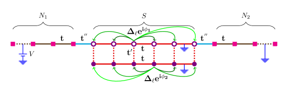
Figure 1: The long range superconducting Kitaev ladder ($S$) is connected to two normal metal leads $N_{1}$ and $N_{2}$. Each of $N_{1}$ and $N_{2}$ is modeled by a one-dimensional tight binding model with a hopping amplitude $t$ and a chemical potential $\mu$. $S$ corresponds to a lattice model as shown and has two coupled parallel long range Kitaev chains. The intra-chain hopping is set to be $t$ and inter-chain hopping is given by $t^{\prime}$ along with on-site chemical potential $\mu$. Each site of each Kitaev chain is connected to every other site in the same Kitaev chain by long range superconducting pairing amplitude $\Delta_{l}e^{i\phi_{\sigma}}=\Delta l^{-\alpha}e^{i\phi_{\sigma}}$ (with long range parameter $\alpha$ where $l$ is the distance between the connecting sites) along with superconducting phase factor $\phi_{\sigma}$ in $\sigma^{th}$ leg of the ladder. The normal metal leads are attached to the upper leg($\sigma=1$) of the ladder with a hopping strength $t^{\prime\prime}$. A voltage bias $V$ is applied from N₁, keeping S and N₂ grounded.

metal, Kitaev ladder and metal.

The rest of the paper is organized as follows. In the next section we introduce the model through a Hamiltonian and discuss the dispersion and the appearance of Majorana modes. The following section describes the transport properties of the long-range Kitaev ladder when it is connected to metallic leads, in relation to the properties of the long-range Kitaev ladder. The concluding section summarizes the central findings.

II Long Range Kitaev ladder

II.1 Hamiltonian

The long-range Kitaev ladder (Bhattacharya et al., 2019; Ares et al., 2018; Giuliano et al., 2018) is a system of two parallel spinless p-wave superconductor wires coupled to each other. To study transport across this system, it is useful to consider a three-terminal setup of normal metal-superconductor-normal metal ($N_{1}SN_{2}$) such that the left metal ($N_{1}$) is maintained at a voltage $V$ while the superconductor ($S$), and the right metal ($N_{2}$) are grounded. The superconductor of the setup is hence connected to two normal metals ($N_{1},N_{2}$) with coupling strength $t^{\prime\prime}$ as shown in Fig. 1.

The Hamiltonian for the setup is given by

$$H=H_{N_{1}}+H_{N_{1}S}+H_{S}+H_{N_{2}S}+H_{N_{2}},$$ (1)

where

$$H_{N_{1}}= -t\displaystyle\sum_{j\leq 0}(c_{j+1}^{\dagger}c_{j}+c_{j}^{\dagger}c_{j+1})-\mu\displaystyle\sum_{j\leq 0}c_{j}^{\dagger}c_{j}$$ (2)

$$H_{N_{2}}= -t\displaystyle\sum_{j\geq L+1}(c_{j+1}^{\dagger}c_{j}+c_{j}^{\dagger}c_{j+1})-\mu\displaystyle\sum_{j\geq L+1}c_{j}^{\dagger}c_{j},$$ (3)

are the Hamiltonians for the normal metal leads,

$$H_{N_{1}S}= -t^{\prime\prime}[c_{0}^{\dagger}c_{1,1}+h.c.],$$ (4)

$$H_{N_{2}S}= -t^{\prime\prime}[c_{L+1}^{\dagger}c_{L,1}+h.c.]$$ (5)

are the Hamiltonians that connect the leads to the superconductor, and

$$H_{S}=- \displaystyle\sum_{j=1\atop\sigma=1,2}^{L-1}(tc_{j+1,\sigma}^{\dagger}c_{j,\sigma}+t^{\prime}c_{j,\sigma}^{\dagger}c_{j,\bar{\sigma}}+h.c.)-\displaystyle\sum_{j=1\atop\sigma=1,2}^{L}\mu\Big{(}c_{j,\sigma}^{\dagger}c_{j,\sigma}-\frac{1}{2}\Big{)}-\displaystyle\sum_{j=1\atop\sigma=1,2}^{L-1}\Bigg{[}\displaystyle\sum_{j^{\prime}=j+1}^{L}\Bigg{(}\frac{\Delta}{(j^{\prime}-j)^{\alpha}}e^{i\phi_{\sigma}}c_{j,\sigma}^{\dagger}c_{j^{\prime},\sigma}^{\dagger}+h.c.\Bigg{)}\Bigg{]}$$ (6)

corresponds to the long-range Kitaev ladder. Here, $c^{\dagger}_{j,\sigma}(c_{j,\sigma})$ are fermion creation (annihilation) operators on $j^{th}$ site ($j=1,2,...,L$) of the $\sigma^{th}$ leg ($\sigma,\bar{\sigma}=1,2$) of the ladder with $a=1$ as unit cell length. The fermion creation (annihilation) operators for normal metal leads are given by $c^{\dagger}_{j}~{}(c_{j})$ where $j$ is a site on the left metal (N₁) for $j\leq 0$ and on the right metal ($N_{2}$) for $j\geq L+1$. The hopping along the legs of the Kitaev ladder as well as in the normal metal leads are maintained at $t$ with onsite chemical potential $\mu$. The inter-leg hopping $t^{\prime}$ couples the two legs of the Kitaev ladder. $\Delta_{l}e^{i\phi_{\sigma}}$ is the

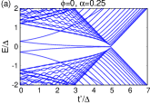
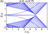
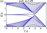
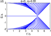
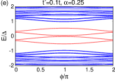
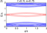
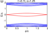
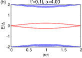
Figure 2: The subgap energy spectrum of the long-range Kitaev ladder with open boundary conditions as a function of (a-d) the inter-leg hopping $t^{\prime}$ with $\phi=0$, and (e-h) the superconducting phase difference ($\phi$) with $t^{\prime}=0.1t$. The other set of parameters are taken to be $\Delta=0.4t$, $\mu=0$ and $L=40$ with long range parameter (a,e) $\alpha=0.25$, (b,f) $\alpha=0.75$, (c,g) $\alpha=1.25$, (d,h) $\alpha=4.00$. The long-range parameter $\alpha\rightarrow\infty$ i.e. large $\alpha$ recovers the short range Kitaev ladder as shown in (d,h). For the lower values of $\alpha$ the Majorana modes split apart as shown in (a-c,e-f). The degeneracy of Majorana zero modes shown by red lines is lifted by breaking of symmetries due to the presence of superconducting phase difference ($\phi$) as well as long-range parameter ($\alpha$).

superconducting pair potential with a constant superconducting phase $\phi_{\sigma}$ in $\sigma^{th}$ leg of the ladder. In this work, we consider a long-range distance-dependent superconducting pair potential (Bhattacharya et al., 2019) $\Delta_{l}=\Delta l^{-\alpha}$ that connects each site of the Kitaev ladder to other sites (in the same leg) as shown in Fig. 1 by green curved lines and decays along the legs of the ladder with distance between two connecting sites ($l=|j-j^{\prime}|$) as a power-law ($\frac{1}{l^{\alpha}}$) with exponent $\alpha>0$. Open boundary conditions, which are natural for the current setup that involves transport from and into metallic leads, are assumed. The contact between metal leads and Kitaev ladder is taken to have a tunable coupling strength $t^{\prime\prime}$.

II.2 Dispersion

In order to study the dispersion and topological properties of the long-range Kitaev ladder, it is convenient to use the Majorana basis (DeGottardi et al., 2011). The fermion operator splits into two Majorana fermion operators:

$$c_{j,\sigma}=\frac{1}{2}(\gamma^{A}_{j,\sigma}+i\gamma^{B}_{j,\sigma}),\;c^{\dagger}_{j,\sigma}=\frac{1}{2}(\gamma^{A}_{j,\sigma}-i\gamma^{B}_{j,\sigma})$$ (7)

where $j$ is the site index of the ladder, $\sigma$ is the leg index of the ladder and $A,B$ are two types of Majorana fermions. In order to maintain the anti-commutator relation of fermions, these Majorana operators should obey the following relations:

$$\gamma^{\eta}_{j,\sigma}=(\gamma^{\eta}_{j,\sigma})^{\dagger},\;\{\gamma^{\eta}_{i,\sigma},\gamma^{\eta^{\prime}}_{j,\sigma^{\prime}}\}=2\delta_{i,j}\delta_{\eta,\eta^{\prime}}\delta_{\sigma,\sigma^{\prime}}$$ (8)

where $\eta,\eta^{\prime}=A,B$, and $\sigma,\sigma^{\prime}=1,2$. The invocation of this unitary transformation in Eq.(6) leads to

$$H_{S}=-\frac{i}{2}\displaystyle\sum_{j=1\atop\sigma=1,2}^{L-1}\Big{[}t(\gamma^{A}_{j+1,\sigma}\gamma^{B}_{j,\sigma}-\gamma^{B}_{j+1,\sigma}\gamma^{A}_{j,\sigma})\Big{]} -\frac{it^{\prime}}{2}\displaystyle\sum_{j=1}^{L}(\gamma^{A}_{j,1}\gamma^{B}_{j,2}+\gamma^{B}_{j,2}\gamma^{A}_{j,1})-\frac{i\mu}{2}\displaystyle\sum_{j=1\atop\sigma=1,2}^{L}(\gamma^{A}_{j,\sigma}\gamma^{B}_{j,\sigma})$$ (9)

$$-\frac{i\Delta}{2}\displaystyle\sum_{j=1\atop\sigma=1,2}^{L-1}\displaystyle\sum_{j^{\prime}=j+1}^{L}\Bigg{[}\frac{\sin\phi_{\sigma}}{(j^{\prime}-j)^{\alpha}} (\gamma^{A}_{j^{\prime},\sigma}\gamma^{A}_{j,\sigma}+\gamma^{B}_{j,\sigma}\gamma^{B}_{j^{\prime},\sigma})+\frac{\cos\phi_{\sigma}}{(j^{\prime}-j)^{\alpha}}(\gamma^{A}_{j,\sigma}\gamma^{B}_{j^{\prime},\sigma}+\gamma^{B}_{j,\sigma}\gamma^{A}_{j^{\prime},\sigma})\Bigg{]}.$$

Further, we take the limit of $L\to\infty$ for the dispersion relation to make sense. A Fourier transformation of the Hamiltonian (with the basis spinor chosen to be $[\gamma^{A}_{k,1},\gamma^{A}_{k,2},\gamma^{B}_{k,1},\gamma^{B}_{k,2}]$) in Eq.(9) results in

$$H_{s}(k)=\begin{bmatrix}Q_{k}&A_{k}\\ A^{\dagger}_{k}&-Q_{k}\end{bmatrix}$$ (10)

where

$$A_{k}=-\frac{i}{2}\begin{bmatrix}(\epsilon_{k}-\Delta_{k}\cos\phi_{1})&t^{\prime}\\ t^{\prime}&(\epsilon_{k}-\Delta_{k}\cos\phi_{2})\end{bmatrix},$$ (11)

$$Q_{k}=-\frac{i}{2}\begin{bmatrix}\Delta_{k}\sin\phi_{1}&0\\ 0&\Delta_{k}\sin\phi_{2}\end{bmatrix},$$ (12)

$\epsilon_{k}=(2t\cos ka+\mu)$, $\Delta_{k}=2i\Delta f_{\alpha}(k)$, $f_{\alpha}(k)=\displaystyle\sum_{l=1}^{\infty}\frac{\sin(kal)}{l^{\alpha}}$, and $a$ is the lattice spacing. The dispersion relation of the isolated long range Kitaev ladder Hamiltonian is given by

$$E=\pm\sqrt{\epsilon_{k}^{2}+{t^{\prime}}^{2}+|\Delta_{k}|^{2}\pm 2t^{\prime}\sqrt{\epsilon_{k}^{2}+|\Delta_{k}|^{2}~{}\sin^{2}\frac{\phi}{2}}},$$ (13)

where $\phi=\phi_{1}-\phi_{2}$ is the superconducting phase difference between the two legs of the ladder. These phases can be managed by superconducting quantum interference devices (SQUIDS) (Wakatsuki et al., 2014b).

The spectrum of the long-range Kitaev ladder is depicted in Fig. 2 when open boundary conditions are imposed for different $\alpha$. In the large $\alpha$ limit i.e. $\alpha\rightarrow\infty$ the system behaves as a short-range Kitaev ladder as shown in Fig. 2(d,h). The gap region of the short-range Kitaev ladder in the absence of superconducting phase difference ($\phi=0$) features four degenerate zero energy Majorana modes in Fig. 2(d). These zero energy Majorana modes are highly localized on the edges of the ladder as compared to any other state of the system which shows dispersive behavior. Each leg of the ladder hosts one Majorana fermion at each end. A finite length of the ladder $L$ couples the Majorana fermions (MFs) at the two ends of the legs of the ladder and they split in energy with a splitting proportional to $e^{-L/l_{0}}$ (Kitaev, 2001), where $l_{0}$ is the decay length in the ladder. However, the presence of the superconducting phase difference enhances the hybridization of Majorana modes of the different legs of the ladder; as a result, the degeneracy of these Majorana fermions is lifted by an amount $E=\pm\tilde{t}\sin{\frac{\phi}{2}}$ as shown by red lines in Fig. 2(h), where $\tilde{t}\sim t^{\prime}$ is the effective coupling between the Majorana fermions of the individual legs of the ladder. These states formed by the hybridization of Majorana fermions are called Andreev bound states (ABSs). The other eigenstates are bulk states of the system and are called subgap Andreev states, which have been shown to be important for non-local transport Soori and Mukerjee (2017); Nehra et al. (2019). These subgap Andreev states (SASs) formed by the hybridization of the bulk bands of the individual legs of the ladder are shown by blue lines in Fig. 2(h).

The long-range nature of the pairings controlled by $\alpha$ has important effects on both Andreev bound states as well as on subgap Andreev states. As $\alpha$ is decreased the system shifts into the long range limit where every site of the ladder is connected to the all other sites by the superconducting term. This connection enhances the decay length of localized Majorana modes inside the bulk of the ladder. This results in splitting of Majorana states due to the coupling of the Majorana states (Andreev bound states) at the two ends of the ladder as shown in Fig. 2(a) (Fig. 2(e)). When $\alpha$ is very small and the system is truly long-ranged, the degeneracy of the MFs (ABSs) is completely lifted even for very tiny $t^{\prime}$. Moreover, as the pairings become more and more long-ranged, the subgap Andreev states have a tendency to close in into the gapped region as illustrated in Fig. 2(a-c,e-g). In between the extreme short-range limit and the extreme long-range limit the Majorana modes remain close to degenerate for small values of $t^{\prime}$ as shown in Fig. 2(d,c) and very strong inter-leg coupling is needed to lift this degeneracy.

II.3 Topological Properties

One of the distinguishing features of the Kitaev system is its topological properties, and can help improve our understanding of the localization domains of the Majorana modes. The Kitaev ladder in the absence of superconducting phase has all three symmetries i.e. particle-hole symmetry, chiral symmetry, and time-reversal symmetry (Kitaev, 2001). A system following these symmetries belongs to the BDI class for which the number of zero energy modes is calculated by a $\mathbb{Z}$ value topological invariant winding number $w$. To calculate the winding number of the Kitaev ladder (Maiellaro et al., 2018; Alecce and Dell’Anna, 2017) with $\phi=0$, the transformed Hamiltonian in Eq.( 10) is converted into off-diagonal form. The winding number ($w$) for such a system is given by

$$w=\frac{1}{2\pi i}\int_{-\pi}^{\pi}dk\Bigg{(}\frac{\partial\;\ln\;\det\;A_{k}}{\partial k}\Bigg{)}.$$ (14)

The winding number ($w$) for the case $\phi=0$ is represented in Fig. 3(a). For $\phi=0$ the winding number of the system takes the values $2,1,0$ depending on the choice of the system parameters. The maximum winding number of $2$ corresponds to the case when two Majorana modes are present at each end of the ladder. When a non-zero superconducting phase difference ($\phi\neq 0$) is present, the Hamiltonian breaks the time-reversal symmetry, and therefore the chiral symmetry as well. Therefore in the presence of superconducting phase difference $\phi$ the system only possesses the particle hole symmetry and thus falls in class D of the classification (Alecce and Dell’Anna, 2017).

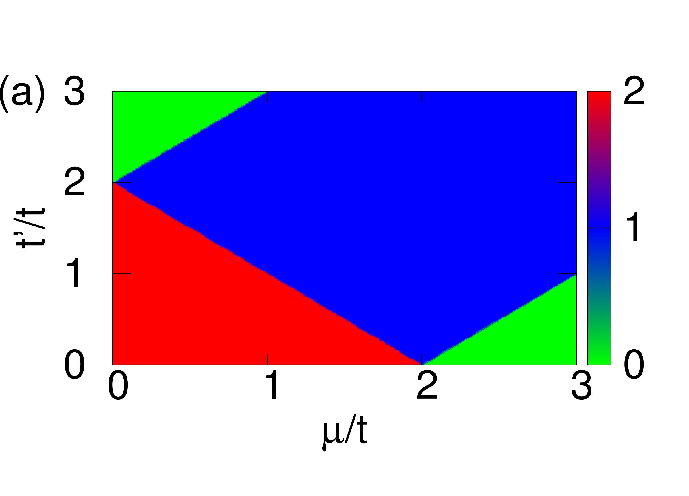
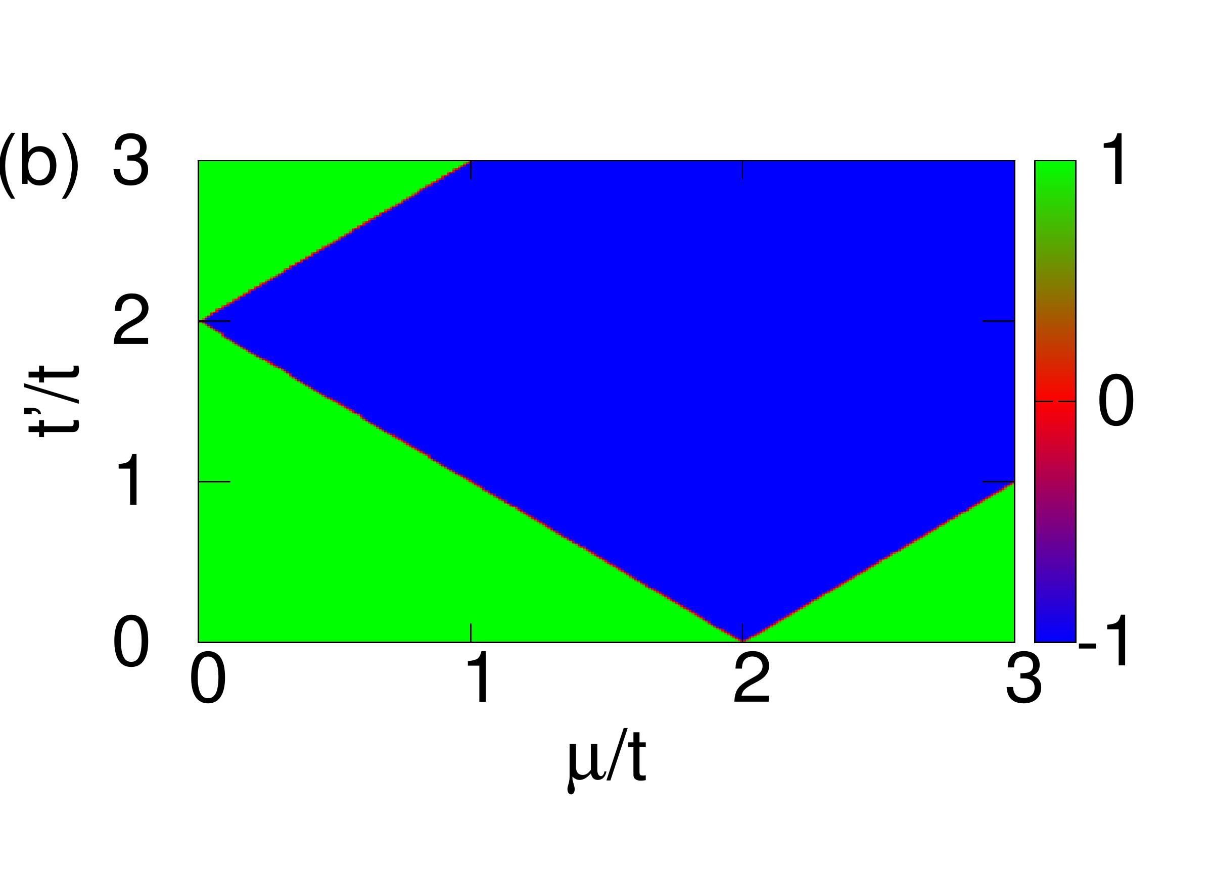
Figure 3: (a) The winding number ($w$ in Eq. 14) for the Kitaev ladder in the limit $\phi=0$ with varying inter-leg hopping and on-site chemical potential $\mu$ with $t=\Delta$. (b) The Majorana number ($M$ in Eq. 15) for the Kitaev ladder for $\phi\neq 0$ with varying inter-leg hopping and on-site chemical potential $\mu$. The green region in both cases shows the non-topological phase and the blue region signifies the presence of at most one Majorana mode at each end of the ladder. The red region corresponds to the presence of at most two Majorana modes per edge.

For class D, the $\mathbb{Z}_{2}$ value Majorana number($M$) is a good topological invariant which involves the calculation of the Hamiltonian’s (Eq. 10) Pfaffian (Kitaev, 2001; Maiellaro et al., 2018; Wu, 2012):

$$M=\operatorname{sgn}(\mathrm{Pf}[H_{s}(0)])\operatorname{sgn}(\mathrm{Pf}[H_{s}(\pi)]).$$ (15)

The Majorana number takes the values $M=1$, and $M=-1$ for non-topological and topological phase, respectively. The Majorana number for the system with $\phi\neq 0$ is depicted in Fig. 3(b) which shows a clear transition from non-topological to topological phase as the different parameters of the system are tuned. We see therefore that in this case, there will be at most one Majorana fermion at the edge of the ladder. We emphasize that the topological features of the long-range Kitaev ladder are completely independent of the parameter $\alpha$.

III Transport

We now study transport in this system with a focus on the role played by the Majorana modes and subgap Andreev states, which have contrasting tendencies. An incident electron must undergo one of four different scattering processes: reflection as an electron, reflection as a hole, transmission as an electron or transmission through the system as a hole. These processes are called Electron reflection (ER), Andreev reflection (AR), Electron tunneling (ET) and crossed Andreev reflection (CAR), respectively. Therefore, considering these different processes, the wave function (on site indexed $j$) in $N_{1}$ and $N_{2}$ can be written as $[\psi^{e}_{j},~{}\psi^{h}_{j}]^{T}$ where

$$\psi^{e}_{j} = e^{ik_{e}aj}+r_{e}e^{-ik_{e}aj}{~{}~{}\rm for~{}~{}}j\leq 0$$

$$\psi^{h}_{j} = r_{h}e^{ik_{h}aj}{~{}~{}\rm for~{}~{}}j\leq 0$$

$$\psi^{e}_{j} = t_{e}e^{ik_{e}aj}{~{}~{}\rm for~{}~{}}j\geq L+1$$

$$\psi^{h}_{j} = t_{h}e^{-ik_{h}aj}{~{}~{}\rm for~{}~{}}j\geq L+1.$$ (16)

In the ladder region, the wave function has the form $[\psi^{e}_{j,\sigma},\psi^{h}_{j,\sigma}]^{T}$ with $1\leq j\leq L$ as the site index and $\sigma=1,2$ as the ladder leg index. At a given energy $E$, $k_{e/h}a=\cos^{-1}\big{[}{(-\mu\mp E)}/{2t}\big{]}$. The scattering amplitudes $r_{e}$, $r_{h}$, $t_{e}$, $t_{h}$ for ER, AR, ET and CAR respectively can be calculated from the equation of motion combined with the form of wavefunction in Eq. (16) as discussed in the appendix.

The local conductance $G_{11}$ is the ratio of the differential change in current in N₁ to the differential change in applied voltage in N₁, i.e., $G_{11}=\frac{dI_{1}}{dV_{1}}$. The nonlocal conductance (or transconductance) is the ratio of the differential change in the current in N₂ to the differential change in the applied voltage in N₁, i.e., $G_{21}=\frac{dI_{2}}{dV_{1}}$. These conductances can be expressed in terms of various scattering probabilities using Landauer-Büttiker formalism Landauer (1957, 1970); Büttiker et al. (1985); Büttiker (1986); Datta (1995) as

$$G_{11} =\frac{e^{2}}{h}\Big{[}1-|r_{e}|^{2}+|r_{h}|^{2}\frac{\sin{k_{h}a}}{\sin{k_{e}a}}\Big{]},$$

$$G_{21} =\frac{e^{2}}{h}\Big{[}|t_{e}|^{2}-|t_{h}|^{2}\frac{\sin{k_{h}a}}{\sin{k_{e}a}}\Big{]}.$$ (17)

As expected, the local processes ER and AR contribute towards local conductance whereas the nonlocal processes ET and CAR contribute towards nonlocal conductance. Further, dominance of AR over ER is signaled by $G_{11}>e^{2}/h$ while dominance of CAR over ET is signaled by a negative $G_{21}$.

III.1 Local transport

Now we turn to the conductance results when the ladder is connected to the two normal metals and a bias is applied from $N_{1}$ grounding the ladder and $N_{2}$. In Fig. 4, the variation of the local conductance ($G_{11}$) as a function of the bias voltage $eV$ and the phase difference ($\phi$) is shown when both the normal metal leads are connected to the Kitaev ladder with coupling strength $t^{\prime\prime}$. First up, we observe that signatures of the Majorana modes are masked in Fig. 4(b,d,f) whereas they are clearly visible in Fig. 4(a,c,e). This indicates that as the coupling $t^{\prime\prime}$ between the leads and the system is increased, perfect AR happens at most energies and the energy of the Andreev bound states is not special. In the short-range limit strongly dominating AR ($G_{11}\sim 2e^{2}/h$) along the lines $eV=\pm\tilde{t}\sin{\frac{\phi}{2}}$ within the bound $|eV|<\Delta$ as depicted in Fig. 4(e) characterize the effect of the ABSs formed at the ends of the ladder. One can see a direct resemblance between Fig. 2(e,f,g) and Fig. 4(a,c,e) respectively. For all the parameters in Fig. 4 we see that $G_{11}$ tends to be relatively small in the region $|eV|>\Delta$ due to presence of the subgap Andreev states. Long-range pairings (as $\alpha$ is decreased) tend to destroy the localization of the MFs and ABSs in the system. The extension of the Andreev bound states into the bulk of the system, in turn suppresses the local transport in the system as depicted in Fig. 4(a,c).

Figure 4: The local conductance $G_{11}$ in units of $e^{2}/h$ as a function of bias voltage $V$ and the superconducting phase difference ($\phi$) with connection strength (a,c,e) $t^{\prime\prime}=0.3t$, (b,d,f) $t^{\prime\prime}=t$, for system parameters $\Delta=0.4t$, $t^{\prime}=0.1t$, $\mu=0$ and $L=40$. The long range parameter is taken to be (a,b) $\alpha=0.25$, (c,d) $\alpha=0.75$ and (e,f) $\alpha=1.25$. (a,c,e) The peak in the local conductance captures the Majorana modes formed by the hybridization of MFs on two legs of the ladder. (b,d,f) The local conductance is unable to provide sharp signatures for the Majorana modes due to the strong coupling between metal leads and superconductor. (a,b) Further, the long-range pairing ($\alpha$ small) hybridizes the Majorana edge modes which destroy their edge localization in the long-range limit $\alpha<<1$. (e,f) The system retains its Majorana edge modes on increasing $\alpha>>1$ which corresponds to the short-range limit of the Kitaev ladder.

Moreover, as $\alpha$ is decreased the lifting of the degeneracy between the Majorana modes is evident, as was also clear from the energy spectrum shown in Fig. 2 (a,b). Though the local conductance $G_{11}$ in Fig. 4(a,c) is peaked in the energy range of the Andreev bound states, the value is below $e^{2}/h$ making it doubtful whether AR happens or not.

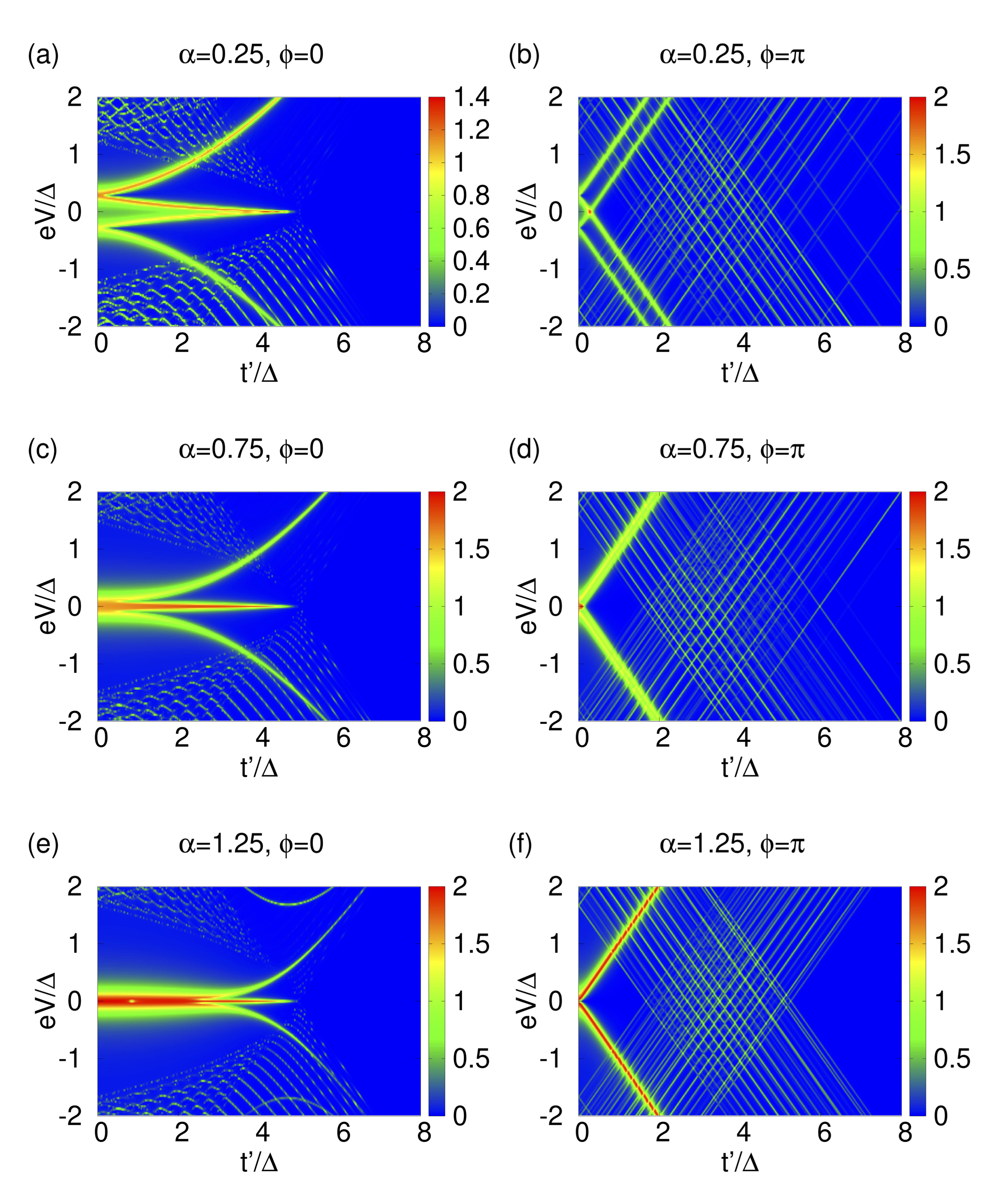
Figure 5: The local conductance $G_{11}$ in units of $e^{2}/h$ as a function of bias voltage $V$ and the inter-leg hopping $t^{\prime}$ with superconducting phase difference (a,c,e)$\phi=0$, (b,d,h) $\phi=\pi$ for the choice of system parameters $\Delta=0.4t$, $t^{\prime\prime}=0.3t$, $\mu=0$ and $L=40$ along with the long-range parameters (a,b) $\alpha=0.25$, (c,d) $\alpha=0.75$ and (e,f) $\alpha=1.25$.

Fig. 2(h) shows that when a non-zero $\phi$ is present for a finite hopping $t^{\prime}$, a lifting of the four-fold degenerate Majorana states by the formation of Andreev bound states is observed. Long-range pairing further lifts the remaining degeneracy, as we have already observed in Fig. 2(e) and Fig. 4(a). It is instructive to study the dependence of the local conductance as a function of the inter-wire hopping $t^{\prime}$. In Fig. 5 the behavior of local conductance as a function of bias voltage $V$ and the inter-wire hopping $t^{\prime}$ with two different values of $\phi$ and for a range of values $\alpha$ is depicted. The local conductance for $\phi=0$ in Fig. 5(a,c,e) shows close resemblance to the energy spectrum of the isolated Kitaev ladder shown in Fig. 2(a-c). We find that along the green lines for $\alpha=0.25$, the local conductance in Fig. 5(a) is very close to $0.8e^{2}/h$ implying a possible lack of AR. But on making the system less long-ranged with $\alpha=0.75$ the local conductance($G_{11}$) is enhanced to a value $\sim 1.25e^{2}/h$ as shown in Fig. 5(c) confirming a dominant AR. As the system tends to become more and more short-ranged, the Majorana modes remain degenerate for small values of $t^{\prime}$ as shown in Fig. 5(e). Thus, the local conductance in the limit of small $t^{\prime}$ and large $\alpha$ shows strong AR with a conductance value $2e^{2}/h$. For higher inter-leg coupling strength the system is still not able to maintain perfectly localized Majorana modes and local conductance also features lack of perfect AR as shown in Fig. 5(e). For $\phi=\pi$, at finite $t^{\prime}$ the MFs in the two legs of the ladder hybridize to form Andreev bound states and a finite $\alpha$ couples the ABSs at two ends of the ladder. In the short-range limit these Andreev bound states cause a split in the degenerate energy by an amount $\sim 2t^{\prime}/\Delta$ which is clearly captured by local transport in Fig. 5(f). For $\phi=\pi$, the ladder dispersion becomes $E=\pm(\sqrt{\epsilon_{k}^{2}+|\Delta_{k}|^{2}}+\nu t^{\prime})$, where $\nu=\pm 1$. In the case of short-range pairing, $\Delta_{k}=2\Delta\sin{ka}$. So, for $t^{\prime}\gtrsim 2\Delta$, the gap closes and hence the features in the region $t^{\prime}\gtrsim 2\Delta$ are due to subgap Andreev states as shown in Fig. 5(b,d,f). Further, the lifting of degeneracy of the ABSs when the pairing becomes long-ranged is captured nicely by local conductance ($G_{11}$) as depicted in Fig. 5(b,d).

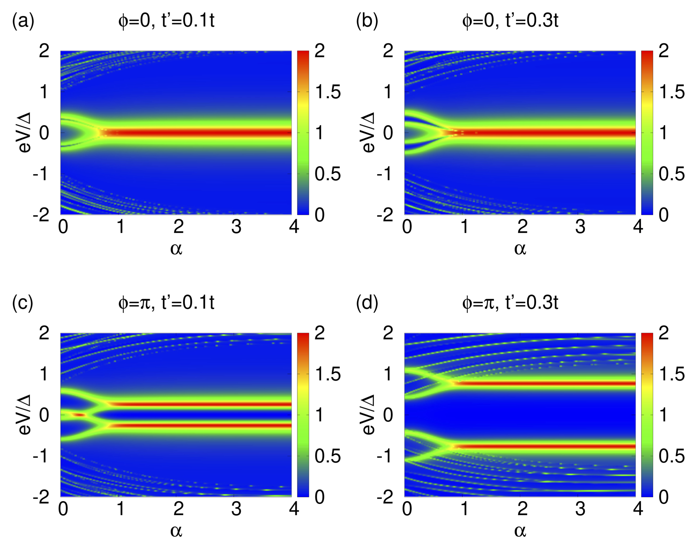
Figure 6: The local conductance $G_{11}$ in units of $e^{2}/h$ as a function of bias voltage $V$ and the long-range parameter $\alpha$ with (a,b) $\phi=0$, (c,d) $\phi=\pi$ for other system parameters $\Delta=0.4t$, $t^{\prime\prime}=0.3t$, $\mu=0$ and $L=40$ along with inter-leg hopping (a,c) $t^{\prime}=0.1t$ and (b,d) $t^{\prime}=0.3t$. The effective short range limit shifts further away from $\alpha=1$ for strong inter-leg coupling strength.

The long-range pairing results in hybridized non-degenerate MFs and ABSs at the two ends of the ladder. Here we look closely at variation of local conductance as a function of the long-range parameter $\alpha$. The transport characteristics of the Kitaev ladder with various $\alpha$ is depicted in Fig. 6. For small inter-leg hopping, short-range behavior seems to be obtained for $\alpha\gtrsim 1$ as shown in Fig. 6(a). This is in line with the results obtained for the long-range Kitaev chain (DeGottardi et al., 2011). As the inter-leg hopping $t^{\prime}$ is increased, a greater critical value of $\alpha$ seems to be needed before the system displays short-range behavior as shown in Fig. 6(b). In Fig. 6(a) the system shows a break in degeneracy of Majorana modes for $\alpha<1$ as the local conductance attains a value $\sim 0.7e^{2}/h$. But for $\alpha>1$ the extreme value $2e^{2}/h$ of local conductance shows the strong presence of AR. Again, in the presence of strong inter-leg hopping $t^{\prime}$ we see that the critical value $\alpha_{c}$ above which degeneracy remains intact is shifted to a greater value as shown in Fig. 6(b).

$\textbf{S.}\atop\textbf{No.}$	$\mathbf{\alpha}$	$\textbf{Degeneracy~{}}\atop\textbf{of~{}MFs}$	$\textbf{Local}\atop\textbf{Conductance}$
1.	$\alpha\lesssim 0.5$	0	$\sim 0.7e^{2}/h$(low AR)
2.	$0.5\lesssim\alpha\lesssim 1.25$	2	$\sim 1.4e^{2}/h$(medium AR)
3.	$\alpha\gtrsim 1.25$	4	$\sim 2e^{2}/h$(high AR)

Table 1: Different degenerate states of the system for different long-range parameter $\alpha$ with $\phi=0,t^{\prime}=0.3t$.

For $t^{\prime}=0.3t$ the system possesses three phases discussed in Table 1. For a nonzero phase difference $\phi$ in the extreme short-range limit $\alpha\rightarrow\infty$ the presence of the inter-leg hopping is itself sufficient to partially lift the four-fold degeneracy of the Majorana modes, making them two-fold degenerate corresponding to each end of the ladder.

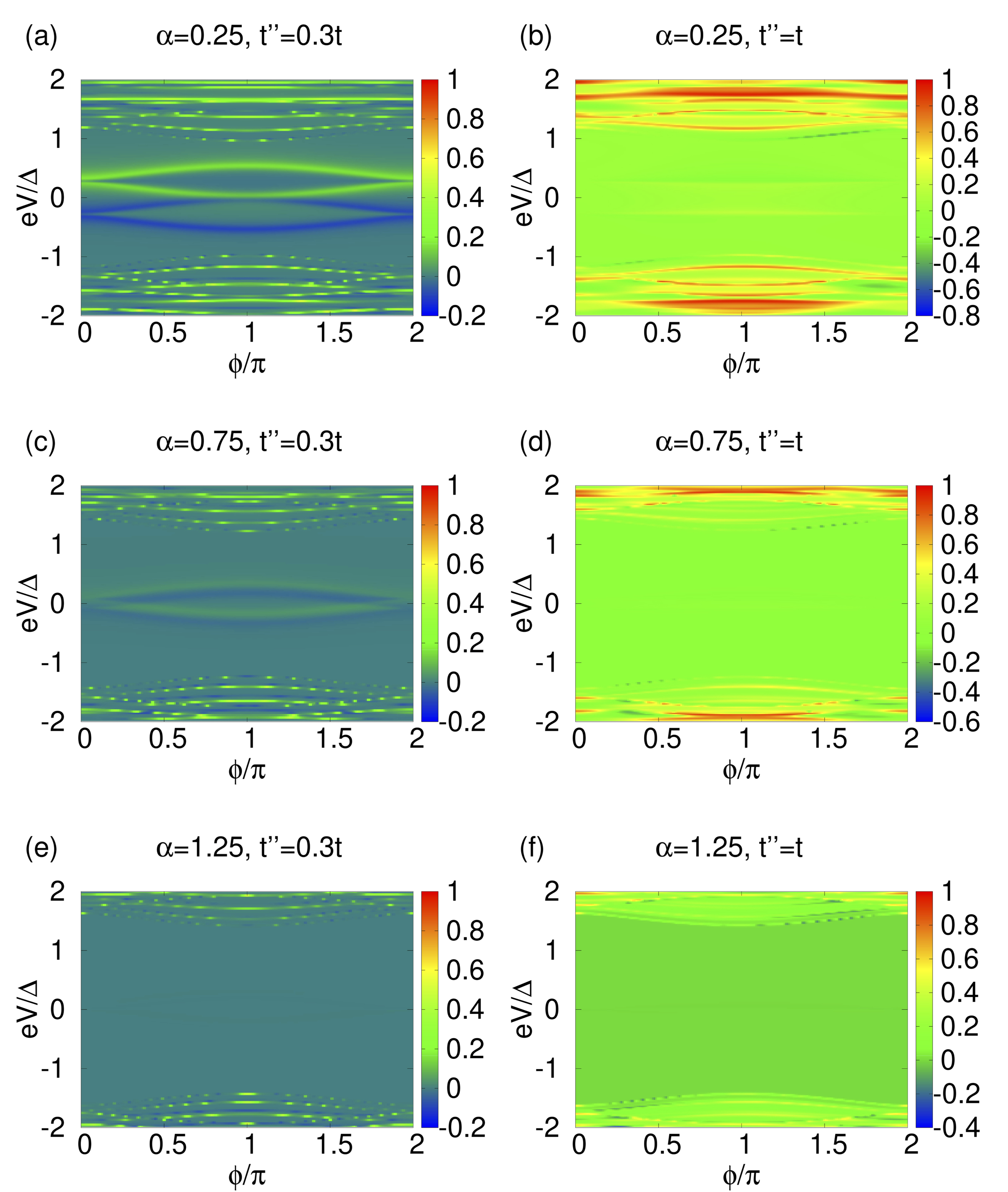
Figure 7: The transconductance $G_{21}$ in units of $e^{2}/h$ as a function of bias voltage $V$ and the superconducting phase difference $\phi$ for system parameters $\Delta=0.4t$, $\mu=0$, $t^{\prime}=0.1t$, $L=40$ and (a,b) $\alpha=0.25$, (c,d) $\alpha=0.75$, (e,f) $\alpha=1.25$ along with (a,c,e) $t^{\prime\prime}=0.3t$ and (b,d,f) $t^{\prime\prime}=t$.

The ABSs formed are split in energy which can be seen in Fig. 2(h), as is also captured by local conductance in Fig. 6(c,d). Further we see from Fig. 6(c,d) that a large inter-leg hopping facilitates the full lifting of degeneracy of the ABSs in a much more effective way, in the long-range pairing regime.

III.2 Nonlocal transport

Before we conclude, we include a short discussion of non-local transport with the help of a study of transconductance ($G_{21}$) in this system. The presence of the highly localized Majorana fermions and Andreev bound states suppresses non-local transport. On the other hand, the long-range pairing ($\alpha$ small) enhances the decay length of Majorana fermions(MFs) and Andreev bound states in the Kitaev ladder, thus aiding non-local transport. Non-local transport is greatly aided by a strong coupling between the normal metals and superconductor Nehra et al. (2019), so for this part of the study we fix $t^{\prime\prime}=t$.

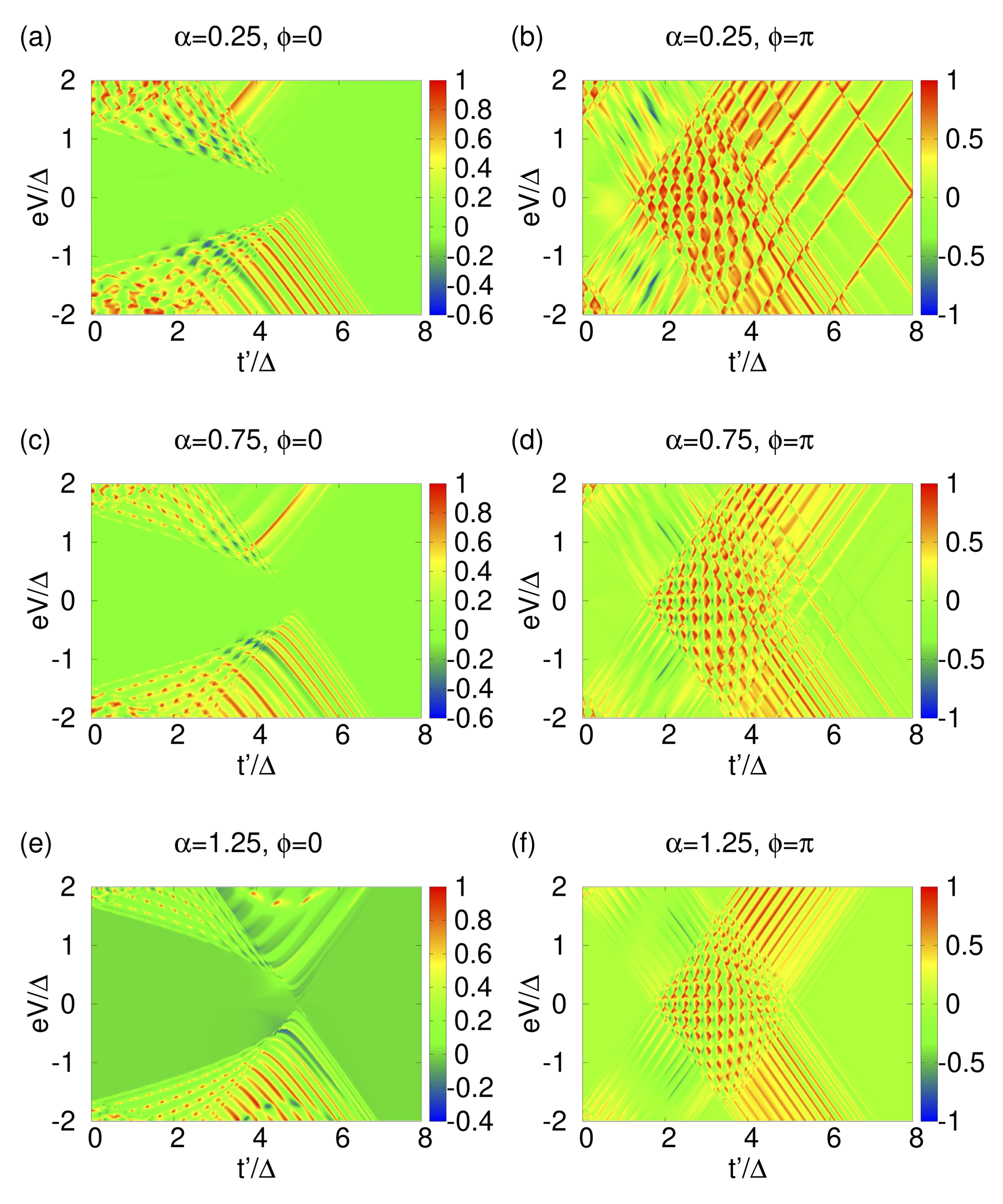
Figure 8: The transconductance $G_{21}$ in units of $e^{2}/h$ as a function of bias voltage $V$ and the inter-leg hopping $t^{\prime}$ for system parameters $\Delta=0.4t$, $\mu=0$, $t^{\prime\prime}=t$, $L=40$ and (a,c,e) $\phi=0$, (b,d,f) $\phi=\pi$. The long-range parameter varies as (a,b) $\alpha=0.25$, (c,d) $\alpha=0.75$ and (e,f) $\alpha=1.25$. The subgap Andreev states mediate the electron tunneling and crossed Andreev reflection through the Kitaev ladder.

The dispersion spectrum in Fig. 2(e-h) shows that the long-range pairing causes the subgap Andreev states to be squeezed within the superconducting gap region. These subgap Andreev states are responsible for non-local transport in the system (Nehra et al., 2019; Soori and Mukerjee, 2017). Fig. 7 studies transconductance as a function of bias and the phase difference for different $\alpha$ and $t^{\prime\prime}$. From Fig. 7 (a) it can be seen that a pair of nonlocal Andreev bound states mediate CAR which dominates over electron tunneling (ET). Also, the long-range pairing favors negative values of transconductance though small in magnitude. In Fig. 8, the behavior of transconductance is studied as a function of inter-leg hopping $t^{\prime}$ and bias voltage $V$. The enhancement in CAR and ET are mediated by subgap Andreev states near the boundary of the biasing window. It is interesting to note from Fig. 8(a,c,e) that long-range pairing can enhance CAR over ET making the transconductance negative even in the absence of superconducting phase difference $\phi$ Nehra et al. (2019). The presence of superconducting phase $\phi$ further shows dominance of CAR over ET in Fig. 8(b,d,f) along the energies of Andreev bound states.

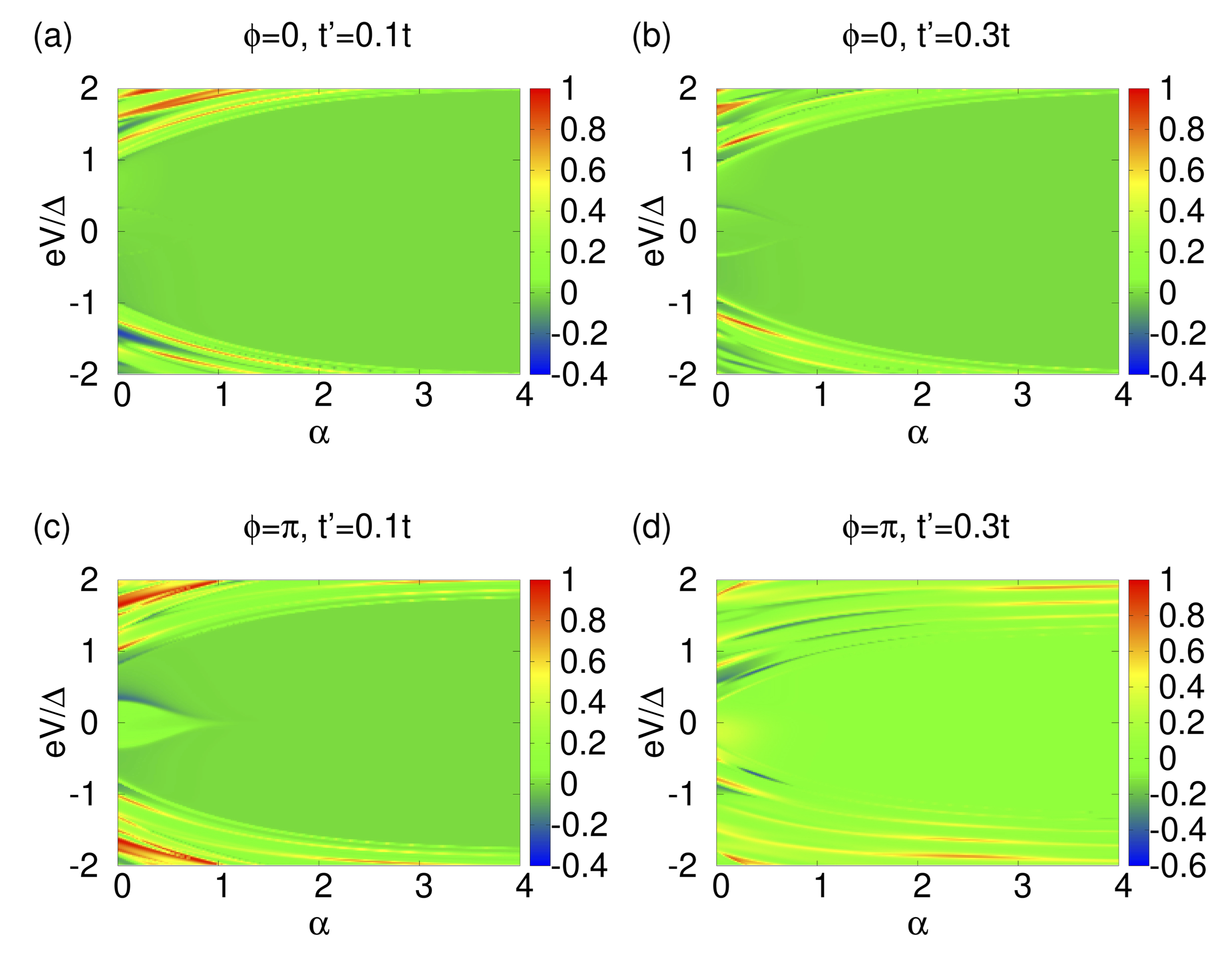
Figure 9: The transconductance $G_{21}$ in units of $e^{2}/h$ as a function of bias voltage $V$ and the long-range parameter $\alpha$ for system parameters $\Delta=0.4t$, $t^{\prime\prime}=t$, $\mu=0$, $L=40$ and (a,c) $t^{\prime}=0.1t$, (b,d) $t^{\prime}=0.3t$ for (a,b) $\phi=0$, (c,d) $\phi=\pi$.

Fig. 9 features the transconductance ($G_{21}$) for a range of $\alpha$ and bias voltage $V$. It can be seen that an enhancement of CAR with nearly extreme values $\sim-0.6e^{2}/h$ of transconductance at some special points is possible in the long-range limits along with superconducting phase $\phi$ and inter-leg hopping $t^{\prime}$.

IV Summary

In this paper, we have studied the connection between the equilibrium and topological properties of a long-range Kitaev ladder and transport through it when the system is connected to metallic leads. Depending on the value of the long-range parameter $\alpha$, the system becomes either short-ranged or long-ranged. The superconducting phase difference breaks different symmetries in the system resulting in a change of the topological class of the Kitaev long-range ladder; however, topological properties are unaffected by the long-range nature of the pairing. Next, we studied local and nonlocal transport through the Kitaev ladder, when it is connected to two normal metals. The isolated long-range Kitaev ladder hosts Andreev bound states formed by a recombination of Majorana end modes and standing waves formed by a recombination of subgap Andreev states. These states mediate local and nonlocal transport respectively. The local conductance is enhanced except for certain parameter choices signaling a dominant Andreev reflection in the short-range limit. Andreev reflection is suppressed by long-range pairing (when $\alpha$ is small) and inter-wire hopping. We also find that long-range pairing alone can enhance crossed Andreev reflection without the need of a superconducting phase difference proposed earlier Nehra et al. (2019); Soori and Mukerjee (2017). For weak normal metal Kitaev ladder hopping, the dependence of local conductance on superconducting phase difference shows the splitting of Majorana state energies and the bands of subgap Andreev states. Thus, we have studied the effect of Andreev bound states formed by the hybridization of Majorana fermions and subgap Andreev states on local and nonlocal transport in the normal metal-Kitaev ladder-normal metal system. While the enhancement of Andreev reflection due to Majorana states is well known, we show that these states can enhance nonlocal transport when the metal-ladder interface hopping is strong though the magnitude of transconductance is low. For strong inter-wire hopping, nonlocal conductance (mediated by subgap Andreev states) is strongly enhanced for certain choices of the parameters.

Appendix A Equation of motion at the boundaries

The appendix contains the detailed calculation of the various scattering amplitudes of all four processes. The wavefunction in two normal metal regions on $j^{th}$ site is given by $[\psi^{e}_{j},~{}\psi^{h}_{j}]^{T}$ where

$$\psi^{e}_{j}= e^{ik_{e}aj}+r_{e}e^{-ik_{e}aj}\quad\text{for}\quad j\leq 0$$ (18)

$$\psi^{h}_{j}= r_{h}e^{ik_{h}aj}\quad\text{for}\quad j\leq 0$$ (19)

$$\psi^{e}_{j}= t_{e}e^{ik_{e}aj}\quad\text{for}\quad j\geq L+1$$ (20)

$$\psi^{h}_{j}= t_{h}e^{-ik_{h}aj}\quad\text{for}\quad j\geq L+1$$ (21)

Here, $r_{e}$, $r_{h}$ are the reflection coefficients and $t_{e}$, $t_{h}$ are the transmission coefficients of electrons and holes in the two metallic leads. Also, momenta of electron and hole are given by $k_{e}a=\cos^{-1}\big{(}\frac{E+\mu}{2t}\big{)}$ and $k_{h}a=\cos^{-1}\big{(}\frac{E-\mu}{2t}\big{)}$ respectively. In the ladder region, the wave function has the form $[\psi^{e}_{j,\sigma},\psi^{h}_{j,\sigma}]^{T}$ with $1\leq j\leq L$ as the site index and $\sigma=1,2$ as the ladder leg index. Here, $a$ is the lattice spacing. There are total $4L+4$ unknowns i.e. wavefunctions in ladder region and 4 scattering coefficients. Also, for a given energy we have $4L+4$ equation of motion at boundaries and in ladder region. These unknowns can be calculated by writing the equations of motion from the Hamiltonian (Eq. 1) at the two boundaries and in ladder region. These equations of motion at the left metal - ladder junction are given by:

$$E\psi_{0}^{e}=-t^{\prime\prime}\psi_{1}^{e}-t\psi_{-1}^{e}-\mu\psi_{0}^{e}$$ (22)

$$E\psi_{0}^{h}=t^{\prime\prime}\psi_{1}^{h}+t\psi_{-1}^{h}+\mu\psi_{0}^{h}.$$ (23)

The equations of motion for upper leg($\sigma=1$) of the long-range Kitaev ladder at a given energy $E$ are

$$E\psi_{1,1}^{e}=-t\psi_{2,1}^{e}-t^{\prime\prime}\psi_{0}^{e}-\mu\psi_{1,1}^{e}-t^{\prime}\psi_{1,2}^{e}-\displaystyle\sum_{j^{\prime}=2}^{L}\frac{\Delta e^{i\phi_{1}}}{(j^{\prime}-1)^{\alpha}}\psi_{j^{\prime},1}^{h}$$ (24)

$$E\psi_{2,1}^{e}=-t(\psi_{1,1}^{e}+\psi_{3,1}^{e})-\mu\psi_{2,1}^{e}-t^{\prime}\psi_{2,2}^{e}-\displaystyle\sum_{j^{\prime}=3}^{L}\frac{\Delta e^{i\phi_{1}}}{(j^{\prime}-2)^{\alpha}}\psi_{j^{\prime},1}^{h}+\Delta e^{i\phi_{1}}\psi_{1,1}^{h}$$ (25)

$$\hskip 20.0pt\vdots\hskip 80.0pt\vdots\hskip 80.0pt\vdots$$

$$E\psi_{L-1,1}^{e}=-t(\psi_{L-2,1}^{e}+\psi_{L,1}^{e})-\mu\psi_{L-1,1}^{e}-t^{\prime}\psi_{L-1,2}^{e}+\displaystyle\sum_{j^{\prime}=1}^{L-2}\frac{\Delta e^{i\phi_{1}}}{(L-1-j^{\prime})^{\alpha}}\psi_{j^{\prime},1}^{h}-\Delta e^{i\phi_{1}}\psi_{L,1}^{h}$$ (26)

$$E\psi_{L,1}^{e}=-t^{\prime\prime}\psi_{L+1}^{e}-t\psi_{L-1,1}^{e}-\mu\psi_{L,1}^{e}-t^{\prime}\psi_{L,2}^{e}+\displaystyle\sum_{j^{\prime}=1}^{L-1}\frac{\Delta e^{i\phi_{1}}}{(L-j^{\prime})^{\alpha}}\psi_{j^{\prime},1}^{h}$$ (27)

$$E\psi_{1,1}^{h}=t\psi_{2,1}^{h}+t^{\prime\prime}\psi_{0}^{h}+\mu\psi_{1,1}^{h}+t^{\prime}\psi_{1,2}^{h}+\displaystyle\sum_{j^{\prime}=2}^{L}\frac{\Delta e^{-i\phi_{1}}}{(j^{\prime}-1)^{\alpha}}\psi_{j^{\prime},1}^{e}$$ (28)

$$E\psi_{2,1}^{h}=t(\psi_{1,1}^{h}+\psi_{3,1}^{h})+\mu\psi_{2,1}^{h}+t^{\prime}\psi_{2,2}^{h}+\displaystyle\sum_{j^{\prime}=3}^{L}\frac{\Delta e^{-i\phi_{1}}}{(j^{\prime}-2)^{\alpha}}\psi_{j^{\prime},1}^{e}-\Delta e^{-i\phi_{1}}\psi_{1,1}^{e}$$ (29)

$$\hskip 20.0pt\vdots\hskip 80.0pt\vdots\hskip 80.0pt\vdots$$

$$E\psi_{L-1,1}^{h}=t(\psi_{L-2,1}^{h}+\psi_{L,1}^{h})+\mu\psi_{L-1,1}^{h}+t^{\prime}\psi_{L-1,2}^{h}-\displaystyle\sum_{j^{\prime}=1}^{L-2}\frac{\Delta e^{-i\phi_{1}}}{(L-1-j^{\prime})^{\alpha}}\psi_{j^{\prime},1}^{e}+\Delta e^{-i\phi_{1}}\psi_{L,1}^{e}$$ (30)

$$E\psi_{L,1}^{h}=t^{\prime\prime}\psi_{L+1}^{h}+t\psi_{L-1,1}^{h}+\mu\psi_{L,1}^{h}+t^{\prime}\psi_{L,2}^{h}-\displaystyle\sum_{j^{\prime}=1}^{L-1}\frac{\Delta e^{-i\phi_{1}}}{(L-j^{\prime})^{\alpha}}\psi_{j^{\prime},1}^{e}.$$ (31)

The equations of motion for lower leg($\sigma=2$) of the long-range Kitaev ladder with incoming energy $E$ of the particle are

$$E\psi_{1,2}^{e}=-t\psi_{2,2}^{e}-\mu\psi_{1,2}^{e}-t^{\prime}\psi_{1,1}^{e}-\displaystyle\sum_{j^{\prime}=2}^{L}\frac{\Delta e^{i\phi_{2}}}{(j^{\prime}-1)^{\alpha}}\psi_{j^{\prime},2}^{h}$$ (32)

$$E\psi_{2,2}^{e}=-t(\psi_{1,2}^{e}+\psi_{3,2}^{e})-\mu\psi_{2,2}^{e}-t^{\prime}\psi_{2,1}^{e}-\displaystyle\sum_{j^{\prime}=3}^{L}\frac{\Delta e^{i\phi_{2}}}{(j^{\prime}-2)^{\alpha}}\psi_{j^{\prime},2}^{h}+\Delta e^{i\phi_{2}}\psi_{1,2}^{h}$$ (33)

$$\hskip 20.0pt\vdots\hskip 80.0pt\vdots\hskip 80.0pt\vdots$$ (34)

$$E\psi_{L-1,2}^{e}=-t(\psi_{L-2,2}^{e}+\psi_{L,2}^{e})-\mu\psi_{L-1,2}^{e}-t^{\prime}\psi_{L-1,1}^{e}+\displaystyle\sum_{j^{\prime}=1}^{L-2}\frac{\Delta e^{i\phi_{2}}}{(L-1-j^{\prime})^{\alpha}}\psi_{j^{\prime},2}^{h}-\Delta e^{i\phi_{2}}\psi_{L,2}^{h}$$ (35)

$$E\psi_{L,2}^{e}=-t\psi_{L-1,2}^{e}-\mu\psi_{L,2}^{e}-t^{\prime}\psi_{L,1}^{e}+\displaystyle\sum_{j^{\prime}=1}^{L-1}\frac{\Delta e^{i\phi_{2}}}{(L-j^{\prime})^{\alpha}}\psi_{j^{\prime},2}^{h}$$ (36)

$$E\psi_{1,2}^{h}=t\psi_{2,2}^{h}+\mu\psi_{1,2}^{h}+t^{\prime}\psi_{1,1}^{h}+\displaystyle\sum_{j^{\prime}=2}^{L}\frac{\Delta e^{-i\phi_{2}}}{(j^{\prime}-1)^{\alpha}}\psi_{j^{\prime},2}^{e}$$ (37)

$$E\psi_{2,2}^{h}=t(\psi_{1,2}^{h}+\psi_{3,2}^{h})+\mu\psi_{2,2}^{h}+t^{\prime}\psi_{2,1}^{h}+\displaystyle\sum_{j^{\prime}=3}^{L}\frac{\Delta e^{-i\phi_{2}}}{(j^{\prime}-1)^{\alpha}}\psi_{j^{\prime},2}^{e}-\Delta e^{-i\phi_{2}}\psi_{1,2}^{e}$$ (38)

$$\hskip 20.0pt\vdots\hskip 80.0pt\vdots\hskip 80.0pt\vdots$$

$$E\psi_{L-1,2}^{h}=t(\psi_{L-2,2}^{h}+\psi_{L,2}^{h})+\mu\psi_{L-1,2}^{h}+t^{\prime}\psi_{L-1,1}^{h}-\displaystyle\sum_{j^{\prime}=1}^{L-2}\frac{\Delta e^{-i\phi_{2}}}{(L-1-j^{\prime})^{\alpha}}\psi_{j^{\prime},2}^{e}+\Delta e^{-i\phi_{2}}\psi_{L,2}^{e}$$ (39)

$$E\psi_{L,2}^{h}=t\psi_{L-1,2}^{h}+\mu\psi_{L,2}^{h}+t^{\prime}\psi_{L,1}^{h}-\displaystyle\sum_{j^{\prime}=1}^{L-1}\frac{\Delta e^{-i\phi_{2}}}{(L-j^{\prime})^{\alpha}}\psi_{j^{\prime},2}^{e}.$$ (40)

The equations of motion at the right normal metal - ladder junction for a given energy $E$ are:

$$E\psi_{L+1}^{e}=-t\psi_{L+2}^{e}-t^{\prime\prime}\psi_{L}^{e}-\mu\psi_{L+1}^{e}$$ (41)

$$E\psi_{L+1}^{h}=t\psi_{L+2}^{h}+t^{\prime\prime}\psi_{L}^{h}+\mu\psi_{L+1}^{h}.$$ (42)

Different unknowns can be computed by solving these equations. Finally, the conductances can be then calculated from Eq. 17.