SPRING: A Sparsity-Aware Reduced-Precision Monolithic 3D CNN Accelerator
Architecture for Training and Inference

Abstract

Convolutional neural networks (CNNs) outperform traditional machine learning algorithms across a wide range of applications, such as object recognition, image segmentation, and autonomous driving. However, their ever-growing computational complexity makes it necessary to design efficient hardware accelerators. Most CNN accelerators focus on exploring various dataflow styles and designs that exploit computational parallelism. However, potential performance improvement from sparsity (in activations and weights) has not been adequately addressed. The computation and memory footprint of CNNs can be significantly reduced if sparsity is exploited in network evaluations. Therefore, different pruning methods have been proposed to increase sparsity. To take advantage of sparsity, some accelerator designs explore sparsity encoding and evaluation on CNN accelerators. However, sparsity encoding is just performed on activation data or CNN weights and only used in inference. It has been shown that activations and weights also have high sparsity levels during the network training phase. Hence, sparsity-aware computation should also be considered in the training phase. To further improve performance and energy efficiency, some accelerators evaluate CNNs with limited precision. However, this is limited to the inference phase since reduced precision sacrifices network accuracy if used in training. In addition, CNN evaluation is usually memory-intensive, especially during training. The performance bottleneck arises from the fact that the memory cannot feed the computational units enough data, resulting in idling of these computational units and thus low utilization ratios. A 3D memory interface has been used on high-end GPUs to alleviate memory bandwidth shortage. In this article, we propose SPRING, a SParsity-aware Reduced-precision Monolithic 3D CNN accelerator for trainING and inference. SPRING supports both CNN training and inference. It uses a binary mask scheme to encode sparsities in activations and weights. It uses the stochastic rounding algorithm to train CNNs with reduced precision without accuracy loss. To alleviate the memory bottleneck in CNN evaluation, especially during training, SPRING uses an efficient monolithic 3D nonvolatile memory interface to increase memory bandwidth. Compared to Nvidia GeForce GTX 1080 Ti, SPRING achieves 15.6$\times$, 4.2$\times$, and 66.0$\times$ improvements in performance, power reduction, and energy efficiency, respectively, for CNN training, and 15.5$\times$, 4.5$\times$, and 69.1$\times$ improvements in performance, power reduction, and energy efficiency, respectively, for inference.

1 Introduction

Convolutional neural networks (CNNs) excel at various important applications, e.g., image classification, image segmentation, robotics control, and natural language processing. However, their high computational complexity necessitates specially-designed accelerators for efficient processing. Training of CNNs requires an enormous amount of computing power to automatically learn the weights based on a large training dataset. Few ASIC-based CNN training accelerators have been presented [1, 2, 3]. However, graphical processing units (GPUs) typically play a dominant in the training phase as CNN computation essentially maps well to their single-instruction multiple-data (SIMD) units and the large number of SIMD units present in GPUs provide significant computational throughput for training CNNs [4, 5]. In addition, the higher clock speed, bandwidth, and power management capabilities of the Graphics Double Data Rate (GDDR) memory relative to the regular DDR memory make GPUs the de facto accelerator choice for CNN training. On the other hand, CNN inference is more latency- and power-sensitive as an increasing number of applications need real-time CNN evaluations on battery-constrained edge devices. Hence, ASIC- and FPGA-based accelerators have been widely explored for this purpose [6, 7, 8, 9, 10]. However, they can only process low-level CNN operations, such as convolution and matrix multiplication, and lack the flexibility of a general-purpose processor. Although CNN models have evolved rapidly recently, their fundamental building blocks are common and long-lasting. Therefore, the ASIC- and FPGA-based accelerators can efficiently process new CNN models with their domain-specific architectures. FPGA-based accelerators achieve faster time-to-market and enable prototyping of new accelerator designs. Microsoft has used customized FPGA boards, called Catapult [11], in its data centers to accelerate Bing ranking by 2$\times$. An FPGA-based CNN accelerator that uses on-chip memory has been proposed in [12], where a fixed-point representation is used to keep all the weights stored in on-chip memory thus avoiding the need to access external memory. To improve dynamic resource utilization of FPGA-based CNN accelerators, multiple accelerators, each specialized for a specific CNN layer, have been constructed using the same FPGA hardware resource [13]. A convolver design for both the convolutional (CONV) layer and fully-connected (FC) layer has been proposed in [14] to efficiently process CNNs on embedded FPGA platforms. ASIC-based CNN accelerators have better energy efficiency and can be fully customized for CNN applications. In [15], CNNs are mapped entirely within the on-chip memory and the ASIC accelerator is placed close to the image sensor so that all the DRAM accesses are eliminated, leading to a 60$\times$ energy efficiency improvement relative to previous works. A 1D chain ASIC architecture is used in [16] to accelerate the CONV layers since these layers are the most compute-intensive [1]. To speed up the CONV layers, a Fast Fourier Transform-based fast multiplication is used in [17]. This accelerator encodes weights using block-circulant matrices and converts convolutions into matrix multiplications to reduce the computational complexity from $O(n^{2})$ to $O(nlogn)$ and storage complexity from $O(n^{2})$ to $O(n)$. A 3D memory system is used in [18] to reduce memory bandwidth pressure. This enables more chip area to be devoted to processing elements (PEs), thus increasing performance and energy efficiency.

To take advantage of the underlying parallel computing resources of CNN accelerators, an efficient dataflow is necessary to minimize data movement between the on-chip memory and PEs. Unlike the temporal architectures, like SIMD or single-instruction multiple-thread, used in central processing units (CPUs) and GPUs, the Google Tensorflow processing unit (TPU) uses a spatial architecture, called the systolic array [19]. Data flow into arithmetic logic units (ALUs) in a wave and move through adjacent ALUs in order to be reused. In [20], multiple CNN layers are fused and processed so that intermediate data can be kept in on-chip memory, thus obviating the need for external memory access. A fine-grained dataflow accelerator is proposed in [21]. It converts convolution into data preprocessing and matrix multiplication. Data are directly transferred among PEs, without the need for redundant control logic, as opposed to temporal architectures, such as DianNao [22]. In [23], a flexible dataflow architecture is described for efficiently processing different types of parallelism: feature map, neuron, and synapse. A dataflow called row-stationary is used in [24] to reuse data and minimize data movement on a spatial architecture.

Although various dataflow styles and computational parallelism designs have been explored in recent works, the potential speedup from weight/activation sparsity is still underexplored. The computation and memory footprint of CNNs can be significantly reduced if sparsity is exploited during network evaluations. Some recent works utilize sparsity to speed up CNN evaluations [25, 26, 27, 28, 29, 30]. However, they only consider either activation or weight sparsity, and only use sparsity during CNN inference based on various pruning methods. It has been shown that the average network-wide activation sparsity of the well-known AlexNet CNN [31] during its entire training process is 62% (a maximum of 93%) [32]. Therefore, the training process can be significantly accelerated if sparsity is exploited. Another CNN acceleration technique is to use reduced precision to improve performance and energy efficiency. For example, TPU and DianNao use 8-bit and 16-bit fixed-point quantizations, respectively, in CNN evaluations. However, low-precision accelerators are currently mainly used in the inference phase, since CNN training involves gradient computation and propagation that require high-precision floating-point operations to achieve high accuracy. Apart from improving the efficiency of the computational resources employed in CNN accelerators, CNN training also requires a large memory bandwidth to store activations and weights. In the forward pass, activations must be retained in the memory until the backward pass commences in order to compute the error gradients and update weights. Besides, in order to fill the SIMD units of GPUs, a large amount of data is needed from the memory. Hence, 3D memory systems, such as hybrid memory cube (HMC) [33] and high bandwidth memory (HBM) [34], have been used in high-end GPUs to provide significant memory bandwidth for CNN training and to bring processing closer to computing. There are many studies on accelerators with near-memory processing (NMP) or processing in memory (PIM) that aim to reduce the memory transfer overhead [35, 36, 37, 38, 39, 40, 41]. In [42], an NMP-enhanced dual in-line memory module is proposed to reduce the latency of embedding fetching and gather/reduction operations used in recommender deep neural networks (DNNs) that take up 34% of the total execution time of DNN workloads in Facebook datacenters [43]. A PIM accelerator, FloatPIM, is proposed in [44]. It speeds up data movement by enabling parallel data transfer between neighboring blocks.

In this article, we make the following contributions:
1) We propose a novel sparsity-aware CNN accelerator architecture, called SPRING. It encodes activation and weight sparsities with binary masks and uses efficient low-overhead hardware implementations for CNN training and inference.
2) SPRING uses reduced-precision fixed-point operations for both training and inference. A dedicated module is used to implement the stochastic rounding algorithm [45] to prevent accuracy loss during CNN training.
3) SPRING uses an efficient monolithic 3D nonvolatile RAM (NVRAM) interface to provide significant memory bandwidth for CNN processing. This alleviates the performance bottleneck in CNN training since the training process is usually memory-bound [46].

We test the proposed SPRING architecture on seven well-known CNNs in the context of both training and inference. Simulation results show that the average execution time, power dissipation, and energy consumption are reduced by 15.6$\times$, 4.2$\times$, and 66.0$\times$, respectively, for CNN training, and 15.5$\times$, 4.5$\times$, and 69.1$\times$, respectively, for inference, relative to Nvidia GeForce GTX 1080 Ti.

The rest of the article is organized as follows. Section 2 discusses the background information required to understand our sparsity-aware accelerator. Section 3 presents the sparsity-aware reduced-precision accelerator architecture. Section 4 describes our simulation setup and flow. Section 5 presents experimental results obtained on seven typical CNNs. Section 6 discusses the limitations of our work. Section 7 concludes the article.

2 Background

In this section, we discuss the background material necessary for understanding our proposed sparsity-aware reduced-precision accelerator architecture. We first give a primer on CNNs. We then discuss existing sparsity-aware designs. Then, we discuss various CNN training algorithms that use low numerical precision. Finally, we describe an efficient on-chip memory interface that is used for CNN acceleration.

2.1 CNN overview

Although different CNNs have different hyperparameters, such as the number of layers and shapes, they share a similar architecture, as shown in Fig. 1. CNNs are generally composed of five building blocks: CONV layers, activation (ACT) layers, pooling (POOL) layers, batch normalization layers (not shown in Fig. 1), and FC layers. Among these basic components, the CONV and FC layers are the most compute-intensive [1]. We describe them next.

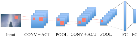
Figure 1: CNN architecture illustration

CONV layers: A batch of 3D input feature maps is convolved with a set of 3D filter weights to generate a batch of 3D output feature maps. The filter weights are usually fetched from external memory once and stored in on-chip memory as they are shared among multiple convolution windows. Therefore, CONV layers have relatively low memory bandwidth pressure and are usually compute-bound as they require a large number of convolution computations. Given the input feature map I and filter weights W, the output feature map O is computed as follows:

$$\begin{split}\textbf{O}[n][k][p][q]={}&\sum\limits_{c=0}^{C-1}\sum\limits_{r=0}^{R-1}\sum\limits_{s=0}^{S-1}\textbf{I}[n][c][p\times u+r][q\times v+s]\\ &\times\textbf{W}[k][c][r][s]\end{split}$$ (1)

where I $\in\mathbb{R}^{NCHW}$, W $\in\mathbb{R}^{KCRS}$, and O $\in\mathbb{R}^{NKPQ}$. $N$ is the number of images in a batch and $K$ is the total number of filters in the CONV layer. $C$ represents the number of channels in the input feature maps and filter weights. $H$ and $W$ denote the height and width of the input feature maps, respectively, whereas $R$ and $S$ denote the height and width of filter weights, respectively. The vertical and horizontal strides are given by $u$ and $v$, respectively. The height and width of the output feature maps are given by $P$ and $Q$, respectively.

FC layers: The neurons in an FC layer are fully connected with neurons in the previous layer with a specific weight associated with each connection. It is the most memory-intensive layer in CNNs [14, 47] since no weight is reused. The computation of the FC layer can be represented by a matrix-vector multiplication as follows:

$$\textbf{y}=\textbf{Wx}+\textbf{b}$$ (2)

where W $\in\mathbb{R}^{m\times n}$, y, b $\in\mathbb{R}^{m}$, and x $\in\mathbb{R}^{n}$. The output and input neurons of the FC layer are represented in vector form as y and x. W represents the weight matrix and b is the bias vector associated with the output neurons.

2.2 Exploiting sparsity in CNN accelerators

It is known that the sparsity levels of CNN weights typically range from 20% to 80% [48, 49], and when the rectified linear unit (ReLU) activation function is employed, the activations are clamped to zeros in the 50% to 70% range [27]. The combination of weight and activation sparsities can reduce computations and memory accesses significantly if the accelerator can support sparsity-aware operations. In order to speed up CNN evaluation by utilizing weight/activation sparsity, the first step is to encode the sparse data in a compressed format that can be efficiently processed by accelerators. EIE is an accelerator that encodes a sparse weight matrix in a compressed sparse column (CSC) format [50] and uses a second vector to encode the number of zeros between adjacent non-zero elements [25]. However, it is only used to speed up the FC layers and has no impact on the CONV layers. Hence, a majority of CNN computations does not benefit from sparsity-aware acceleration. A lightweight run-time output sparsity predictor has been developed in SparseNN, an architecture enhanced from EIE, to accelerate CNN inference [26]. Activations in the CSC format are first fed to the lightweight predictor to predict the non-zero elements in the output neurons. Then, the activations associated with non-zero outputs are sent to feedforward computations to bypass computations that lead to zero outputs. If the number of computations skipped is large enough, the overhead of output predictions can be offset. However, since the output sparsity predicted by the lightweight predictor is an approximation of the real sparsity value, it incurs an accuracy loss that makes it unsuitable for CNN training. SCNN is another accelerator that uses a zero-step format to encode weight/activation sparsity: an index vector is used to indicate the number of non-zero data points and the number of zeros before each non-zero data point. It multiplies activation and weight vectors in a manner similar to a Cartesian product using an input stationary dataflow [27]. However, the Cartesian product does not automatically align non-zero weights and activations in the FC layers since the FC layer weights are not reused as in the case of CONV layers. This leads to performance degradation for FC layers and makes SCNN unattractive for CNNs dominated by FC layers. Stitch-X [51], an improved version of SCNN, adopts a hybrid dataflow by leveraging both spatial and temporal partial-sum reduction to dynamically stitch together non-zero activations and weights. Cnvlutin [29] enhances the DaDianNao architecture to support zero-skipping in activations using a zero-step offset vector that is similar to graphics processor proposals [52, 53, 54, 55]. The limitation of this architecture is that the length of offset vectors in different PEs may be different. Hence, they may require different numbers of cycles to process the data. Thus, the PE with the longest offset vector becomes the performance bottleneck while other PEs idle and wait for it. Cambricon-X is an accelerator that also employs the zero-step sparsity encoding method and uses a dedicated indexing module to select and transfer needed neurons to PEs, with a reduced memory bandwidth requirement [30]. The PEs run asynchronously to avoid the idling problem of Cnvlutin. An enhanced version, Cambricon-S, is then proposed to reduce the irregularity of weight sparsity using a software-based coarse-grained pruning technique [56]. UCNN is an accelerator that improves CNN inference performance by exploiting weight repetition in the CONV layers [28]. It uses a factorized dot product dataflow to reduce the number of multiplications and a memorization method to reduce weight memory access via weight repetition.

Both the CSC and zero-step encoding formats compress data by eliminating zero-elements and the accelerators discussed above efficiently process the compressed data. However, weight/activation sparsity can not only be exploited at the PE level but also at the bit level. Stripes, a bit-serial hardware accelerator, avoids the processing of zero prefix and suffix bits through serial-parallel multiplications on CNNs [57]. Each bit of a neuron is processed at every cycle and zero bits are skipped on the fly. Multiple neurons are processed in parallel to mitigate performance loss from bit-serial processing. Pragmatic, a CNN accelerator enhanced from Stripes, supports zero-bit skipping regardless of its position [58]. However, it needs to convert the input neuron representation into a zero-bit-only format on the fly, which leads to up to a 16-cycle latency.

2.3 Low-precision CNN training algorithms

The rapid evolution of CNNs in recent years has necessitated the deployment of large-scale distributed training using high-performance computing infrastructure [59, 60, 61]. Even with such a powerful computing infrastructure, training a CNN to convergence usually takes several days, sometimes even a few weeks. Hence, to speed up the CNN training process, various training algorithms with low-precision computations have been proposed.

Single-precision floating-point (FP32) operation has mainly been used as the training standard on GPUs. Meanwhile, efforts have been made to train CNNs with half-precision floating-point (FP16) arithmetic since it can improve training throughput by 2$\times$, in theory, on the same computing infrastructure. However, compared to FP32, FP16 involves rounding off gradient values and quantizing to a lower-precision representation. This introduces noise in the training process and defers CNN convergence. To maintain a balance between the convergence rate and training throughput, mixed-precision training algorithms that use a combination of FP32 and FP16 have been proposed [62, 63]. The FP16 representation is used in the most compute-intensive multiplications and the results are accumulated into FP32 outputs. Dynamic scaling is required to prevent the vanishing gradient problem [64].

Compared to floating-point arithmetic, fixed-point operations are much faster and more energy-efficient on hardware accelerators, but have a lower dynamic range. To overcome the dynamic range limitation, the dynamic fixed-point format [65] is used in CNN training [66, 67]. Unlike the regular fixed-point format, the dynamic fixed-point format uses multiple scaling factors that are updated during training to adjust the dynamic range of different groups of variables. The CNN training convergence rate is highly sensitive to the rounding scheme used in fixed-point arithmetic [45]. Instead of tuning the dynamic range used in the dynamic fixed-point format, a stochastic rounding method has been proposed to leverage the noise tolerance of CNN algorithms [45]. CNNs are trained in a manner that the rounding error is exposed to the network and weights are updated accordingly to mitigate this error, without impacting the convergence rate.

2.4 Efficient on-chip memory interface and emerging NVRAM technologies

CNN training involves feeding vast input feature maps and filter weights to the accelerator computing units to compute the error gradients used to update CNN weights in backpropagation. Besides the large memory size required to store all the CNN weights, a high memory bandwidth becomes indispensable to keep running the computing units at full throughput. Hence, through-silicon via (TSV)-based 3D memory interfaces have been used on high-end GPUs [5] and specialized CNN accelerators [3]. The most widely-used TSV-based 3D memory interface is HBM. In each HBM package, multiple DRAM dies and one memory controller die are first fabricated and tested individually. Then, these dies are aligned, thinned, and bonded using TSVs. The HBM package is connected to the processor using an interposer in a 2.5D manner. This shortens the interconnects within the memory system and between the memory and processor, thus reducing memory access latency and improving memory bandwidth. In addition, since more DRAM dies are integrated within the same footprint area, HBM enables smaller form factors: HBM-2 uses 94% less space relative to GDDR5 for a 1GB memory [68].

Apart from improving the DRAM interface, the industry has also been exploring various NVRAM technologies to replace DRAM, such as ferroelectric RAM (FeRAM), spin-transfer torque magnetic RAM (STT-MRAM), phase-change memory (PCM), nanotube RAM (NRAM), and resistive RAM (RRAM). It has been shown in [69, 70] that RRAM can be used in an efficient 3D memory interface to deliver high memory bandwidth and energy efficiency. Information is represented by different resistance levels in an RRAM cell. Compared to a DRAM, an RRAM cell needs a higher current to change its resistance level. Therefore, the access transistors of an RRAM are larger than those of a DRAM [71]. However, DRAM is expected to reach the scaling limit at 16$nm$ [72] whereas RRAM is believed to be suitable for sub-10$nm$ nodes [73]. Hence, the smaller technology node of an RRAM should offset the access transistor overhead. Besides, the nonvolatility of RRAM eliminates the need for a periodic refresh that a DRAM requires. This not only saves energy and reduces latency, but also gets rid of the refresh circuitry used in DRAM.

3 Sparsity-aware reduced-precision accelerator architecture

In this section, we present the proposed architecture, SPRING: a sparsity-aware reduced-precision CNN accelerator for both training and inference. We first discuss accelerator architecture design and then dive into sparsity-aware acceleration, reduced-precision processing, and the monolithic 3D NVRAM interface.

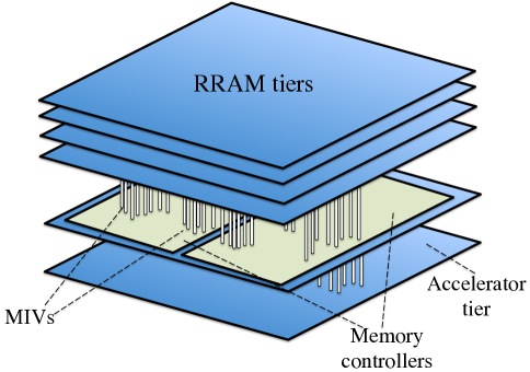
Figure 2: The SPRING architecture

Fig. 2 shows the high-level view of the architecture. SPRING uses monolithic 3D integration to connect the accelerator tier with an RRAM interface. Unlike TSV-based 3D integration, monolithic 3D integration only has one substrate wafer, where devices are fabricated tier over tier. Hence, the alignment, thinning, and bonding steps of TSV-based 3D integration can be eliminated. In addition, tiers are connected through monolithic inter-tier vias (MIVs), whose diameter is the same as that of local vias and one-to-two orders of magnitude smaller than that of TSVs. This enables a much higher MIV density ($10^{8}/mm^{2}$ at 14$nm$ [74]), thus leaving much more space for logic. The accelerator tier is put at the bottom, on top of which is the memory controller tier. Above the memory controller tier lie the multiple RRAM tiers.

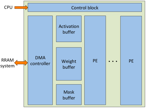
Figure 3: Accelerator organization

Fig. 3 shows the organization of the accelerator tier. The control block handles the CNN configuration sent from the CPU. It fetches the instruction stream and controls the rest of the accelerator to perform acceleration. The activations and filter weights are brought on-chip from the RRAM system by a direct memory access (DMA) controller. Activations and weights are stored in the activation buffer and weight buffer, respectively, in a compressed format. Data compression relies on binary masks that are stored in a dedicated mask buffer. The compression scheme is discussed in Section 3.1. The compressed data and the associated masks are used in the PEs for CNN evaluation. The PEs are designed to operate in parallel to maximize overall throughput.

Fig. 4 shows the main components of a PE. The compressed data are buffered by the activation FIFO and weight FIFO. Then, they enter the pre-compute sparsity module along with the binary masks. Multiple multiplier-accumulator (MAC) lanes are used to compute convolutions or matrix-vector multiplications using zero-free activations and weights after they are preprocessed by the pre-compute sparsity module. The output results go through a post-compute sparsity module to maintain the zero-free format. Batch normalization operations [75] are used in modern CNNs to reduce the covariance shift. They are executed in the batch normalization module that supports both the forward pass and backward pass of batch normalization. Three pooling methods are supported by the pooling module: max pooling, min pooling, and mean pooling. The reshape module deals with matrix transpose and data reshaping. Element-wise arithmetic, such as element-wise add and subtract, is handled by the scalar module. Lastly, a dedicated loss module is used to process various loss functions, such as L1 loss, L2 loss, softmax, etc.

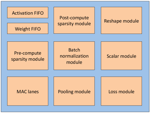
Figure 4: Internal components of a PE

3.1 Sparsity-aware acceleration

Traditional accelerator designs can only process dense data and do not support sparse-encoded computation. They treat zero elements in the same manner as regular data and thus perform operations that have no impact on the CNN evaluation results. In this context, weight/activation sparsity cannot be used to speed up computation and reduce the memory footprint. In order to utilize sparsity to skip ineffectual activations and weights, and reduce the memory footprint, SPRING uses a binary-mask scheme to encode the sparse data and performs computations directly in the encoded format.

Compared to the regular dense format, SPRING compresses data vectors by removing all the zero-elements. In order to retain the shape of the uncompressed data, an extra binary mask is used. The binary mask has the same shape as that of the uncompressed data where each binary bit in the mask is associated with one element in the original data vector. Fig. 5 shows an example of the binary-mask scheme that SPRING uses to compress activations and weights. The original uncompressed data vector has 16 elements, and if each element is represented using 16 bits, the total data length is 256 bits. With the binary scheme, only the six non-zero elements remain. The total length of the compressed data vector and the binary mask is 112 bits, which leads to a compression ratio of 2.3$\times$ for this example.

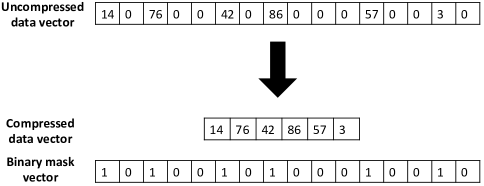
Figure 5: The binary mask scheme: An example

We implement the binary mask scheme using a low overhead pre-compute sparsity module that preprocesses the sparse-encoded activations and weights and provides zero-free data to the MAC lanes. After output data traverse the MAC lanes, another post-compute sparsity module is used to remove all the zero-elements generated by the activation function before storing them back to on-chip memory. Fig. 6 shows the pre-compute sparsity module that takes the zero-free data vectors and binary mask vectors as inputs, and generates an output mask as well as zero-free activations/weights for the MAC lanes. The output binary mask indicates the common indexes of non-zero elements in both the activation and weight vectors. After being preprocessed by the pre-compute sparsity module, the “dangling” non-zero elements in the activation and weight data vectors are removed. The dangling non-zero activations refer to the non-zero elements in the activation data vector where their corresponding weights at the same index are zeros, and vice versa.

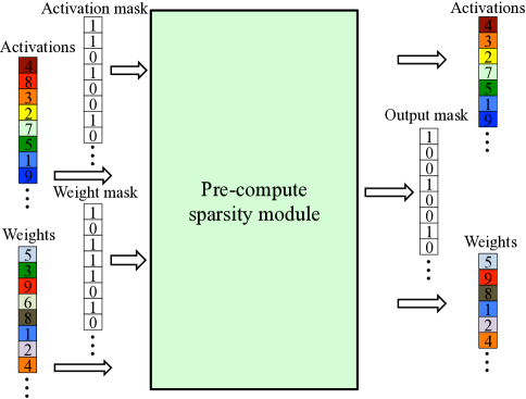
Figure 6: The pre-compute sparsity module

Fig. 7(a) shows the mask generation process used by the pre-compute sparsity module. The output mask is the AND of the activation and weight masks. The output mask, together with the activation and weight masks, is used by two more XOR gates for filter mask generation. Fig. 7(b) shows the dangling data filtering process using the three masks obtained in the previous step. The sequential scanning and filtering mechanism for one type of data used in the filtering step is shown in Algorithm 1. The data vector, as well as the two mask vectors, is scanned in sequence. At each step, a 1 in the output mask implies a common non-zero index. Hence, the corresponding element in the data vector passes through the filter. On the other hand, if a 0 appears in the mask filter and the corresponding mask bit in the filter mask is 1, then a dangling non-zero element is detected in the data vector and is blocked by the filter. If both the output mask bit and filter mask bit are zeros, it means that the data elements at this index in both the activation and weight vectors are zeros and thus already skipped. After filtering out the dangling elements in activations and weights, a zero-collapsing shifter is used to remove the zeros and keep the data vectors zero-free in a similar sequential scanning manner, as shown in Fig. 7(c). These zero-free activations and weights are then fed to the MAC lanes for computation. Since only zero-free data are used in the MAC lanes, ineffectual computations are completely skipped, thus improving throughput and saving energy.

Algorithm 1 Sequential scanning and filtering mechanism

1:Inputs: in_data, output_mask, filter_mask

2:output: out_data

3:data_pointer$\leftarrow$0, mask_pointer$\leftarrow$0

4:while mask_pointer $<$ mask_length do

5:     if output_mask[mask_pointer] == 1 then

6:         out_data[data_pointer] = in_data[data_pointer]

7:         data_pointer++

8:     else if filter_mask[mask_pointer] == 1 then

9:         out_data[data_pointer] = 0

10:         data_pointer++      

11:     mask_pointer++

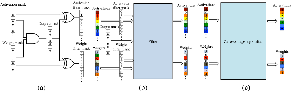
Figure 7: The submodules of the pre-compute sparsity module: (a) mask generation, (b) dangling-data filter, and (c) zero-collapsing shifter

3.2 Reduced-precision processing using stochastic rounding

SPRING processes CNNs using fixed-point numbers with reduced precision. Every time a new result is generated by the CNN, it has to be first rounded to the nearest discrete number, either in a floating-point representation or a fixed-point representation. Since the gap between adjacent numbers in the fixed-point representation is much larger than in the floating-point representation, the resulting quantization error in the former is much more pronounced. This prevents the fixed-point representation from being used in error-sensitive CNN training. In order to utilize the faster and more energy-efficient fixed-point arithmetic units, we adopt the stochastic rounding method proposed in [45]. The traditional deterministic rounding scheme always rounds a real number to its nearest discrete number, as shown in Eq. 3. We follow the definitions used in [45], where $\epsilon$ denotes the smallest positive discrete number supported in the fixed-point format and $\lfloor x\rfloor$ is defined as the largest integer multiple of $\epsilon$ less than or equal to x.

$$Round(x)=\begin{cases}\lfloor x\rfloor&{if\ x<\lfloor x\rfloor+\dfrac{\epsilon}{2}}\\ \lfloor x\rfloor+\epsilon&{otherwise}\end{cases}$$ (3)

In contrast, a real number $x$ is rounded to $\lfloor x\rfloor$ and $\lfloor x\rfloor+\epsilon$ stochastically in the stochastic rounding scheme, as shown in Eq. 4 [45]. It is shown in [45] that with the stochastic rounding scheme, the CNN weights can be trained to tolerate the quantization noise without increasing the number of cycles required for convergence.

$$Round(x)=\begin{cases}\lfloor x\rfloor&{with\ probability\ \dfrac{\lfloor x\rfloor+\epsilon-x}{\epsilon}}\\ \lfloor x\rfloor+\epsilon&{with\ probability\ \dfrac{x-\lfloor x\rfloor}{\epsilon}}\end{cases}$$ (4)

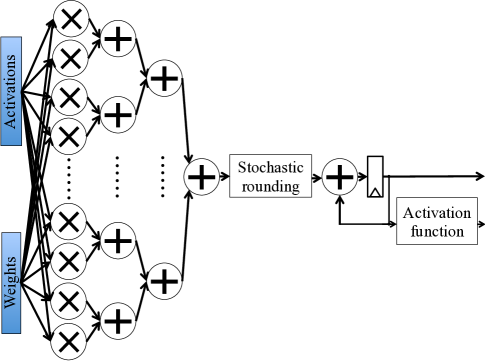
Figure 8: The MAC lane

The stochastic rounding scheme is embedded in the MAC lane, as shown in Fig. 8. Activations and weights are represented using fixed-point numbers using IL+FL bits, where IL denotes the number of bits for the integer portion and FL denotes the number of bits for the fraction part. The zero-free activations and weights from the pre-compute sparsity module are subject to multiplications in the MAC lanes, where the products are represented with 2$\times$IL integer bits and 2$\times$FL fractional bits to prevent overflow. Accumulations over products are also performed using 2$\times$(IL+FL) bits. Then, a stochastic rounding module is used to reduce the numerical precision before applying the activation function or storing the result back to on-chip memory. We use a linear-feedback shift register to generate pseudo-random numbers for stochastic rounding.

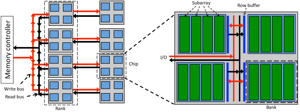
Figure 9: Read/write decoupled interconnects [70]

3.3 Monolithic 3D NVRAM interface

SPRING uses a monolithic 3D NVRAM interface previously proposed in [69] and adapts it to its 3D architecture to provide the accelerator tier with significant memory bandwidth. As shown in Fig. 2, SPRING uses two memory channels where each channel has its own memory controller to control the associated two RRAM ranks. An ultra-wide memory bus (1KB wide) is used in each channel, since the interconnects between SPRING and memory controllers, and between memory controllers and RRAM ranks, are implemented using vertical MIVs. This on-chip memory bus not only reduces the access latency relative to the conventional off-chip memory bus, but also makes row-wide granular memory accesses possible to enable energy savings. In addition, the column decoder can be removed to reduce the access latency and power dissipation in this row-wide access granularity scheme. To reduce repeated accesses to the same row, especially the energy-consuming write accesses of RRAM, the row buffer is reused as the write buffer. A dirty bit is used to indicate if the corresponding row entry in the row buffer needs to be written back to the RRAM array when flushed out. The read and write accesses are decoupled by adding another set of vertical interconnects, as shown in Fig. 9 [70]. Hence, the slower write access does not block the faster read access and thus a higher memory bandwidth is achieved. In addition, RRAM nonvolatility not only enables the elimination of bulky periodic refresh circuitry, but also allows the RRAM arrays to be powered down in the idle intervals to reduce leakage power. A rank-level adaptive power-down policy is used to maintain a balance between performance and energy saving: the power-down threshold for each RRAM rank is adapted to its idling pattern so that a rank is only powered down if it is expected to be idle for a long time.

4 Simulation methodology

In this section, we present the simulation flow for SPRING and the experimental setup.

Fig. 10 shows the simulation flow used to evaluate the proposed SPRING accelerator architecture. We implement components of SPRING at the register-transfer level (RTL) with SystemVerilog to estimate delay, power, and area. The RTL design is synthesized by Design Compiler [76] using a 14nm FinFET technology library [77]. Floorplanning is done by Capo [78], an open-source floorplacer. On-chip buffers are modeled using FinCACTI [79], a cache modeling tool enhanced from CACTI [80], to support deeply-scaled FinFETs at the 14nm technology node. The monolithic 3D RRAM system is modeled by NVSim [81], a circuit-level memory simulator for emerging NVRAMs, and NVMain [82], an emerging NVRAM architecture simulator. The synthesized results, together with buffer and RRAM estimations, are then plugged into a customized cycle-accurate Python simulator. This accelerator simulator takes CNNs in the TensorFlow [83] Protocol Buffers format and estimates the computation latency, power dissipation, energy consumption, and area. SPRING treats the TensorFlow operations like complex instruction set computer instructions where each operation involves many low-level operations and the CNNs are mapped to SPRING using an analytical model similar to the one used in [84].

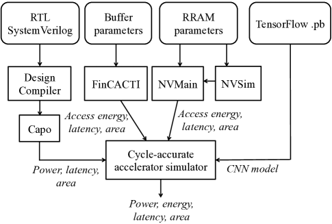
Figure 10: Simulation flow

We compare our design with the Nvidia GeForce GTX 1080 Ti GPU, which uses the Pascal microarchitecture [4] in a 16nm technology node. The die size of GTX 1080 Ti is 471$mm^{2}$ and the base operating frequency is 1.48 $GHz$, which can be boosted to 1.58 $GHz$. GTX 1080 Ti uses an 11 GB GDDR5X memory with 484 GB/s memory bandwidth to provide 10.16 TFLOPS peak single-precision performance.

We evaluate SPRING and GTX 1080 Ti on seven well-known CNNs: Inception-Resnet V2 [85], Inception V3 [86], MobileNet V2 [87], NASNet-mobile [88], PNASNet-mobile [89], Resnet-152 V2 [90], and VGG-19 [91]. We evaluate both the training and inference phases of these CNNs on the ImageNet dataset [92]. The sparsity of the CNNs are assumed to be 50%, as it is shown in [32] that the average sparsity level of widely used CNNs, such as AlexNet [31], VGG [91], and Inception [86], are over 50%. We use the default batch sizes defined in the TensorFlow-Slim library [93]: 32 for training and 100 for inference.

5 Experimental results

In this section, we present experimental results for SPRING and compare them with those for GTX 1080 Ti.

Table I shows the values of various design parameters used in SPRING. They are obtained through the accelerator design space exploration methodology proposed in [84]. It is shown in [45] that with 16 FL bits, training CNNs using the stochastic rounding scheme can converge in a similar amount of time with a negligible accuracy loss relative to when single-precision floating-point arithmetic is used. Hence, we use 4 IL bits and 16 FL bits in the fixed-point representation. The convolution loop order refers to the execution order of the multiple for-loops in the CONV layer. SPRING executes convolutions by first unrolling the for-loops across multiple inputs in the batch. Then, it unrolls the for-loops within the filter weights, followed by unrolling in the activation channel dimension. In the next step, it unrolls the for-loops with activation feature maps. Finally, it unrolls for-loops across the output channels.

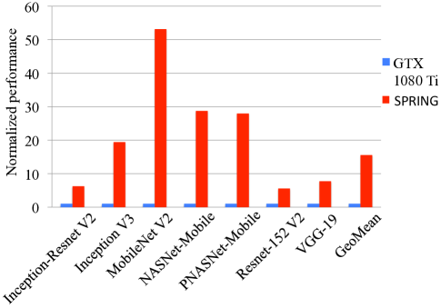
Figure 11: Normalized training performance

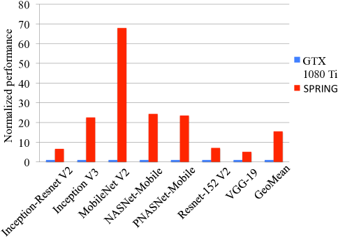
Figure 12: Normalized inference performance

TABLE I: SPRING design parameters

Accelerator parameters	Values
Clock rate	700 $MHz$
Number of PEs	64
Number of MAC lanes per PE	72
Number of multipliers per MAC lane	16
Weight buffer size	24 MB
Activation buffer size	12 MB
Mask buffer size	4 MB
Convolution loop order	batch-weight-in channel-input-out channel
IL bits	4
FL bits	16
Technology	14nm FinFET
Area	151 $mm^{2}$
Monolithic 3D RRAM	8 GB, 2 channels, 2 ranks, 16 banks,
	1 KB bus, $t_{BURST}$=0.5 ns, 2.0 $GHz$ [71]

Fig. 11 and Fig. 12 show the normalized performance of SPRING and GTX 1080 Ti over the seven CNNs in the training and inference phases, respectively. All results are normalized to those of GTX 1080 Ti. In the training phase, SPRING achieves speedups ranging from 5.5$\times$ to 53.1$\times$ with a geometric mean of 15.6$\times$ on the seven CNNs. In the inference phase, SPRING is faster than GTX 1080 Ti by 5.1$\times$ to 67.9$\times$ with a geometric mean of 15.5$\times$. In both cases, SPRING has better performance speedups on relatively light-weight CNNs, i.e., MobileNet V2, NASNet-mobile, and PNASNet-mobile. This is because these light-weight CNNs do not require large volumes of activations and weights to be transferred between the external memory and on-chip buffers. Therefore, the memory bandwidth bottleneck is alleviated and the speedup from sparsity-aware computation becomes more noteworthy. On the other hand, on large CNNs, such as Inception-Resnet V2 and VGG-19, the sparsity-aware MAC lanes of SPRING idle and wait for data fetch from the RRAM system, lowering the performance speedup relative to GTX 1080 Ti.

Fig. 13 and Fig. 14 show the normalized reciprocal of power of SPRING and GTX 1080 Ti in training and inference, respectively. All results are normalized to those of GTX 1080 Ti. On an average, SPRING reduces power dissipation by 4.2$\times$ and 4.5$\times$ for training and inference, respectively.

Fig. 15 and Fig. 16 show the normalized energy efficiency of SPRING and GTX 1080 Ti for training and inference, respectively. All results are normalized to those of GTX 1080 Ti. Compared to the GTX 1080 Ti, SPRING achieves an average of 66.0$\times$ and 69.1$\times$ energy efficiency improvements in training and inference, respectively. This makes the GTX 1080 Ti columns invisible. We observe that, among the seven CNNs, SPRING achieves the best normalized energy efficiency on MobileNet V2, both in the training and inference phases. Since MobileNet V2 has a much smaller network size (97.6% parameter reduction compared to VGG-19 [87]), most of the network weights can be retained in on-chip buffers without accessing the external memory. Hence, SPRING can reduce energy consumption significantly through our sparsity-aware acceleration scheme. On the other hand, energy reduction from sparsity-aware computation is offset by energy-consuming memory accesses on large CNNs, such as Inception-Resnet V2 and VGG-19. This is consistent with the results reported in [30] that show that over 80% of the total energy consumption is from memory access.

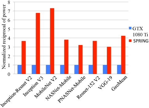
Figure 13: Normalized reciprocal of power for training

Figure 14: Normalized reciprocal of power for inference

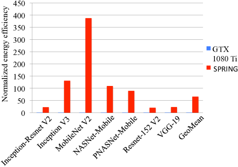
Figure 15: Normalized energy efficiency in training

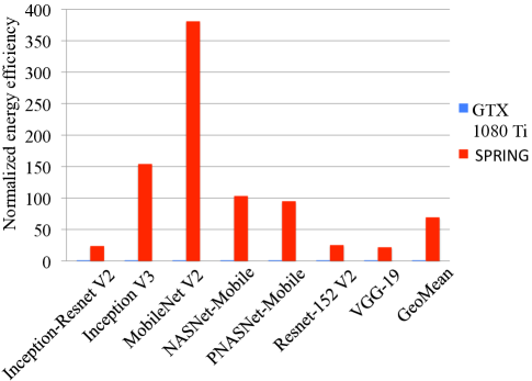
Figure 16: Normalized energy efficiency in inference

6 Discussions and limitations

In this section, we discuss the assumptions we made in this work and the limitations of the SPRING architecture.

The SPRING architecture is based on the assumption that the monolithic 3D stacking technology is emerging in the near future. One main disadvantage of monolithic 3D integration, compared to the TSV-based 3D stacking, is that the high-temperature process used for the top tiers may damage the interconnects on the tiers below. To prevent or minimize this damage, either low-temperature annealing is used for the top tiers or Copper is replaced with Tungsten as the interconnect material on the bottom tiers. However, low-temperature annealing may degrade device performance on the top tiers while the Tungsten interconnect is less competitive with the Copper counterpart in terms of performance on the bottom tiers. However, it is still not clear how the low thermal budget process on the top tiers correlates to the degree of top-tier device degradation for advanced technology nodes [94]. Some previous works assume the devices on the top tiers will be degraded to some extent and evaluate the overall chip performance based on this assumption [95, 96]. On the other hand, there are works suggesting that the degradation is negligible when certain monolithic 3D processes are used [97, 98]. For example, it is shown in [99] that using Tungsten for interconnects on the bottom tiers for interconnect-dominant circuits has a limited impact on overall performance and power consumption (less than 2% degradation in both performance and power consumption). Hence, we do not model the degradation from the monolithic 3D integration process in this work.

The performance speedup, power reduction ratio, and energy efficiency improvement reported in Section 5 are obtained at the batch level. We use batch-level training results since the CNN training results are based on the assumption that with sufficient precision bits, fixed-point training using stochastic rounding scheme can lead to convergence with no worse number of cycles than the training process based on single-precision floating-point arithmetic, as suggested in [45], where 16 FL bits are used for fixed-point training with stochastic rounding and the convergent epoch number is similar to that of single-precision floating-point training.

A major limitation of the SPRING accelerator architecture is that the sequential scanning and filtering mechanism shown in Algorithm 1 needs multiple cycles to filter out dangling non-zero elements and collapse the resulting zeros. This may incur a long latency in data preprocessing, which makes SPRING unsuitable for latency-sensitive edge inference applications. However, since this sequential scanning and filtering scheme is pipelined, the overall throughput is unaffected and therefore the total latency for one batch is independent of the sequential scanning steps used by the pre-compute sparsity module.

Our binary mask encoding method is similar to the dual indexing encoding proposed in [100]. Although we both use a binary mask to point to the index of non-zero elements in the data vector, our binary mask encoding scheme has several advantages. First, the index masks are kept in binary form throughout the entire sparsity encoding and decoding process. Hence, the storage overhead of the binary mask is at most 5%, assuming 4 IL bits and 16 FL bits. The real storage overhead is much lower than this value since most of activations and weights are zeros. However, the binary masks are converted to decimal masks in [100] to serve as select signals of a MUX. This not only increases the storage overhead of the masks, but also increases the computation complexity of mask manipulation. Besides, their binary-to-decimal mask transfer process is sequential, which incurs a long processing latency that increases as the size of the mask vector increases.

While preparing this article, we became aware of a very recent work that shares our motivations but adopts different approaches. Eager Pruning [101], an algorithm-architecture co-design method, speeds up DNN training by moving pruning to the training phase. It is observed in [101] that the ranking of weight magnitudes is relatively stable during the training process. Hence, insignificant weights can be identified and pruned in the early training stage. This reduced training computation is then transformed into speedup through a dedicated accelerator architecture. The sparse weights are distributed to multiple PEs using a Dynamically Reconfigurable Add and Collect Tree (DRACT) to support the dataflow of Eager Pruning. However, Eager Pruning only supports speedup from weight sparsity but lacks support for activation sparsity. The sparsity-aware acceleration scheme discussed in this article can be combined with the Eager Pruning dataflow through the help of DRACT for the full use of data sparsity (both activations and weights).

7 Conclusion

In this article, we proposed a sparsity-aware reduced-precision CNN accelerator, named SPRING. A binary mask scheme is used to encode weight/activation sparsity. It is efficiently processed through a sequential scanning and filtering mechanism. SPRING adopts the stochastic rounding algorithm to train CNNs using reduced-precision fixed-point numerical representation. An efficient monolithic 3D NVRAM interface is used to provide significant memory bandwidth for CNN evaluation. Compared to Nvidia GeForce GTX 1080 Ti, SPRING achieves 15.6$\times$, 4.2$\times$, and 66.0$\times$ improvements in performance, power reduction, and energy efficiency, respectively, in the training phase, and 15.5$\times$, 4.5$\times$, and 69.1$\times$ improvements in performance, power reduction, and energy efficiency, respectively, in the inference phase.

Ye Yu received the B.Eng. degree in Electronic and Computer Engineering from The Hong Kong University of Science and Technology, Hong Kong, China, in 2014, and the M.A. and Ph.D. degrees in Electrical Engineering from Princeton University, NJ, USA, in 2016 and 2019, respectively. He is currently a software engineer at Microsoft. His current research interests include computer vision, machine learning, and deep learning model compression and acceleration.

Niraj K. Jha (S’85-M’85-SM’93-F’98) received his B.Tech. degree in Electronics and Electrical Communication Engineering from Indian Institute of Technology, Kharagpur, in 1981 and Ph.D. degree in Electrical Engineering from University of Illinois at Urbana-Champaign, IL in 1985. He has been a faculty member of the Department of Electrical Engineering, Princeton University, since 1987. He is a Fellow of IEEE and ACM, and was given the Distinguished Alumnus Award by I.I.T., Kharagpur. He has also received the Princeton Graduate Mentoring Award. He has served as the Editor-in-Chief of IEEE Transactions on VLSI Systems and as an Associate Editor of several other journals. He has co-authored five books that are widely used. His research has won 20 best paper awards or nominations. His research interests include smart healthcare, cybersecurity, machine learning, and monolithic 3D IC design. He has given several keynote speeches in the area of nanoelectronic design/test and smart healthcare.

References

- [1] Y. Chen, T. Luo, S. Liu, S. Zhang, L. He, J. Wang, L. Li, T. Chen, Z. Xu, N. Sun, and O. Temam, “DaDianNao: A machine-learning supercomputer,” in Proc. IEEE/ACM Int. Symp. Microarchitecture, Dec. 2014, pp. 609–622.
- [2] S. Venkataramani, A. Ranjan, S. Banerjee, D. Das, S. Avancha, A. Jagannathan, A. Durg, D. Nagaraj, B. Kaul, P. Dubey, and A. Raghunathan, “Scaledeep: A scalable compute architecture for learning and evaluating deep networks,” in Proc. Int. Symp. Computer Architecture, June 2017, pp. 13–26.
- [3] C. Ying, S. Kumar, D. Chen, T. Wang, and Y. Cheng, “Image classification at supercomputer scale,” arXiv preprint arXiv:1811.06992, Dec. 2018.
- [4] D. Foley and J. Danskin, “Ultra-performance Pascal GPU and NVLink interconnect,” IEEE Micro, vol. 37, no. 2, pp. 7–17, Mar. 2017.
- [5] J. Choquette, O. Giroux, and D. Foley, “Volta: Performance and programmability,” IEEE Micro, vol. 38, no. 2, pp. 42–52, Mar. 2018.
- [6] Y. Li, J. Park, M. Alian, Y. Yuan, Z. Qu, P. Pan, R. Wang, A. Schwing, H. Esmaeilzadeh, and N. S. Kim, “A network-centric hardware/algorithm co-design to accelerate distributed training of deep neural networks,” in Proc. IEEE/ACM Int. Symp. Microarchitecture, Oct. 2018, pp. 175–188.
- [7] Y. Shen, M. Ferdman, and P. Milder, “Escher: A CNN accelerator with flexible buffering to minimize off-chip transfer,” in Proc. Int. Symp. Field-Programmable Custom Computing Machines, Apr. 2017, pp. 93–100.
- [8] J. Yu, A. Lukefahr, D. Palframan, G. Dasika, R. Das, and S. Mahlke, “Scalpel: Customizing DNN pruning to the underlying hardware parallelism,” in Proc. Int. Symp. Computer Architecture, June 2017, pp. 548–560.
- [9] H. Sharma, J. Park, N. Suda, L. Lai, B. Chau, V. Chandra, and H. Esmaeilzadeh, “Bit fusion: Bit-level dynamically composable architecture for accelerating deep neural networks,” in Proc. Int. Symp. Computer Architecture, June 2018, pp. 764–775.
- [10] H. Kwon, A. Samajdar, and T. Krishna, “MAERI: Enabling flexible dataflow mapping over DNN accelerators via reconfigurable interconnects,” in Proc. Int. Conf. Architectural Support Programming Languages Operating Syst., Mar. 2018, pp. 461–475.
- [11] A. Putnam, A. M. Caulfield, E. S. Chung, D. Chiou, K. Constantinides, J. Demme, H. Esmaeilzadeh, J. Fowers, G. P. Gopal, J. Gray, M. Haselman, S. Hauck, S. Heil, A. Hormati, J.-Y. Kim, S. Lanka, J. Larus, E. Peterson, S. Pope, A. Smith, J. Thong, P. Y. Xiao, and D. Burger, “A reconfigurable fabric for accelerating large-scale datacenter services,” in Proc. Int. Symp. Computer Architecuture, 2014, pp. 13–24.
- [12] J. Park and W. Sung, “FPGA based implementation of deep neural networks using on-chip memory only,” in Proc. IEEE Int. Conf. Acoustics, Speech, Signal Processing, Mar. 2016, pp. 1011–1015.
- [13] Y. Shen, M. Ferdman, and P. Milder, “Overcoming resource underutilization in spatial CNN accelerators,” in Proc. Int. Conf. Field Programmable Logic Applications, Aug. 2016, pp. 1–4.
- [14] J. Qiu, J. Wang, S. Yao, K. Guo, B. Li, E. Zhou, J. Yu, T. Tang, N. Xu, S. Song, Y. Wang, and H. Yang, “Going deeper with embedded FPGA platform for convolutional neural network,” in Proc. ACM/SIGDA Int. Symp. Field-Programmable Gate Arrays, 2016, pp. 26–35.
- [15] Z. Du, R. Fasthuber, T. Chen, P. Ienne, L. Li, T. Luo, X. Feng, Y. Chen, and O. Temam, “ShiDianNao: Shifting vision processing closer to the sensor,” in Proc. ACM/IEEE Int. Symp. Computer Architecture, June 2015, pp. 92–104.
- [16] S. Wang, D. Zhou, X. Han, and T. Yoshimura, “Chain-NN: An energy-efficient 1D chain architecture for accelerating deep convolutional neural networks,” in Proc. Design, Automation Test Europe Conf. Exhibition, Mar. 2017, pp. 1032–1037.
- [17] C. Ding, S. Liao, Y. Wang, Z. Li, N. Liu, Y. Zhuo, C. Wang, X. Qian, Y. Bai, G. Yuan, X. Ma, Y. Zhang, J. Tang, Q. Qiu, X. Lin, and B. Yuan, “CirCNN: Accelerating and compressing deep neural networks using block-circulant weight matrices,” in Proc. IEEE/ACM Int. Symp. Microarchitecture, Oct. 2017, pp. 395–408.
- [18] M. Gao, J. Pu, X. Yang, M. Horowitz, and C. Kozyrakis, “TETRIS: Scalable and efficient neural network acceleration with 3D memory,” in Proc. Int. Conf. Architectural Support Programming Languages Operating Syst., 2017, pp. 751–764.
- [19] N. P. Jouppi, C. Young, N. Patil, D. Patterson, G. Agrawal, R. Bajwa, S. Bates, S. Bhatia, N. Boden, A. Borchers, R. Boyle, P.-l. Cantin, C. Chao, C. Clark, J. Coriell, M. Daley, M. Dau, J. Dean, B. Gelb, T. V. Ghaemmaghami, R. Gottipati, W. Gulland, R. Hagmann, C. R. Ho, D. Hogberg, J. Hu, R. Hundt, D. Hurt, J. Ibarz, A. Jaffey, A. Jaworski, A. Kaplan, H. Khaitan, D. Killebrew, A. Koch, N. Kumar, S. Lacy, J. Laudon, J. Law, D. Le, C. Leary, Z. Liu, K. Lucke, A. Lundin, G. MacKean, A. Maggiore, M. Mahony, K. Miller, R. Nagarajan, R. Narayanaswami, R. Ni, K. Nix, T. Norrie, M. Omernick, N. Penukonda, A. Phelps, J. Ross, M. Ross, A. Salek, E. Samadiani, C. Severn, G. Sizikov, M. Snelham, J. Souter, D. Steinberg, A. Swing, M. Tan, G. Thorson, B. Tian, H. Toma, E. Tuttle, V. Vasudevan, R. Walter, W. Wang, E. Wilcox, and D. H. Yoon, “In-datacenter performance analysis of a tensor processing unit,” in Proc. Int. Symp. Computer Architecture, June 2017, pp. 1–12.
- [20] M. Alwani, H. Chen, M. Ferdman, and P. Milder, “Fused-layer CNN accelerators,” in Proc. IEEE/ACM Int. Symp. Microarchitecture, Oct. 2016, pp. 1–12.
- [21] T. Xiang, Y. Feng, X. Ye, X. Tan, W. Li, Y. Zhu, M. Wu, H. Zhang, and D. Fan, “Accelerating CNN algorithm with fine-grained dataflow architectures,” in Proc. IEEE Int. Conf. High Performance Computing Communications; IEEE Int. Conf. Smart City; IEEE Int. Conf. Data Science Syst., June 2018, pp. 243–251.
- [22] T. Chen, Z. Du, N. Sun, J. Wang, C. Wu, Y. Chen, and O. Temam, “DianNao: A small-footprint high-throughput accelerator for ubiquitous machine-learning,” in Proc. Int. Conf. Architectural Support Programming Languages Operating Syst., Mar. 2014, pp. 269–284.
- [23] W. Lu, G. Yan, J. Li, S. Gong, Y. Han, and X. Li, “Flexflow: A flexible dataflow accelerator architecture for convolutional neural networks,” in Proc. IEEE Int. Symp. High Performance Computer Architecture, Feb. 2017, pp. 553–564.
- [24] Y. Chen, J. Emer, and V. Sze, “Eyeriss: A spatial architecture for energy-efficient dataflow for convolutional neural networks,” in Proc. ACM/IEEE Int. Symp. Computer Architecture, June 2016, pp. 367–379.
- [25] S. Han, X. Liu, H. Mao, J. Pu, A. Pedram, M. A. Horowitz, and W. J. Dally, “EIE: Efficient inference engine on compressed deep neural network,” in Proc. Int. Symp. Computer Architecture, June 2016, pp. 243–254.
- [26] J. Zhu, J. Jiang, X. Chen, and C. Tsui, “SparseNN: An energy-efficient neural network accelerator exploiting input and output sparsity,” in Proc. Design, Automation Test Europe Conf. Exhibition, Mar. 2018, pp. 241–244.
- [27] A. Parashar, M. Rhu, A. Mukkara, A. Puglielli, R. Venkatesan, B. Khailany, J. Emer, S. W. Keckler, and W. J. Dally, “SCNN: An accelerator for compressed-sparse convolutional neural networks,” in Proc. ACM/IEEE Int. Symp. Computer Architecture, June 2017, pp. 27–40.
- [28] K. Hegde, J. Yu, R. Agrawal, M. Yan, M. Pellauer, and C. W. Fletcher, “UCNN: Exploiting computational reuse in deep neural networks via weight repetition,” in Proc. Int. Symp. Computer Architecture, June 2018, pp. 674–687.
- [29] J. Albericio, P. Judd, T. Hetherington, T. Aamodt, N. E. Jerger, and A. Moshovos, “Cnvlutin: Ineffectual-neuron-free deep neural network computing,” in Proc. ACM/IEEE Int. Symp. Computer Architecture, June 2016, pp. 1–13.
- [30] S. Zhang, Z. Du, L. Zhang, H. Lan, S. Liu, L. Li, Q. Guo, T. Chen, and Y. Chen, “Cambricon-X: An accelerator for sparse neural networks,” in Proc. IEEE/ACM Int. Symp. Microarchitecture, Oct. 2016, pp. 1–12.
- [31] A. Krizhevsky, I. Sutskever, and G. E. Hinton, “Imagenet classification with deep convolutional neural networks,” in Proc. Int. Conf. Neural Information Processing Syst., Dec. 2012, pp. 1097–1105.
- [32] M. Rhu, M. O’Connor, N. Chatterjee, J. Pool, Y. Kwon, and S. W. Keckler, “Compressing DMA engine: Leveraging activation sparsity for training deep neural networks,” in Proc. IEEE Int. Symp. High Performance Computer Architecture, Feb. 2018, pp. 78–91.
- [33] HMC Consortium. (2014) Hybrid Memory Cube specification 2.1. [Online]. Available: http://hybridmemorycube.org/files/SiteDownloads/HMC-30G-VSR_HMCC_Specification_Rev2.1_20151105.pdf
- [34] Samsung Newsroom. (2016) Samsung begins mass producing world’s fastest DRAM - based on newest High Bandwidth Memory (HBM) interface. [Online]. Available: https://www.samsung.com/semiconductor/insights/news-events/samsung-begins-mass-producing-worlds-fastest-dram-based-on-newest-high-bandwidth-memory-hbm/
- [35] M. Alian, S. W. Min, H. Asgharimoghaddam, A. Dhar, D. K. Wang, T. Roewer, A. McPadden, O. O’Halloran, D. Chen, J. Xiong, D. Kim, W. Hwu, and N. S. Kim, “Application-transparent near-memory processing architecture with memory channel network,” in Proc. IEEE/ACM Int. Symp. Microarchitecture, Oct. 2018, pp. 802–814.
- [36] H. Asghari-Moghaddam, Y. H. Son, J. H. Ahn, and N. S. Kim, “Chameleon: Versatile and practical near-DRAM acceleration architecture for large memory systems,” in Proc. IEEE/ACM Int. Symp. Microarchitecture, Oct. 2016, pp. 1–13.
- [37] P. Chi, S. Li, C. Xu, T. Zhang, J. Zhao, Y. Liu, Y. Wang, and Y. Xie, “PRIME: A novel processing-in-memory architecture for neural network computation in ReRAM-based main memory,” in Proc. Int. Symp. Computer Architecture, June 2016, pp. 27–39.
- [38] D. Kim, J. Kung, S. Chai, S. Yalamanchili, and S. Mukhopadhyay, “Neurocube: A programmable digital neuromorphic architecture with high-density 3D memory,” SIGARCH Computer Architecture News, vol. 44, no. 3, pp. 380–392, June 2016.
- [39] A. Shafiee, A. Nag, N. Muralimanohar, R. Balasubramonian, J. P. Strachan, M. Hu, R. S. Williams, and V. Srikumar, “ISAAC: A convolutional neural network accelerator with in-situ analog arithmetic in crossbars,” in Proc. Int. Symp. Computer Architecture, June 2016, pp. 14–26.
- [40] M. Cheng, L. Xia, Z. Zhu, Y. Cai, Y. Xie, Y. Wang, and H. Yang, “TIME: A training-in-memory architecture for memristor-based deep neural networks,” in Proc. ACM/EDAC/IEEE Design Automation Conf., June 2017, pp. 1–6.
- [41] S. Gupta, M. Imani, H. Kaur, and T. S. Rosing, “NNPIM: A processing in-memory architecture for neural network acceleration,” IEEE Trans. Computers, vol. 68, no. 9, pp. 1325–1337, Sep. 2019.
- [42] Y. Kwon, Y. Lee, and M. Rhu, “TensorDIMM: A practical near-memory processing architecture for embeddings and tensor operations in deep learning,” in Proc. IEEE/ACM Int. Symp. Microarchitecture, Oct. 2019, pp. 740–753.
- [43] J. Park, M. Naumov, P. Basu, S. Deng, A. Kalaiah, D. Khudia, J. Law, P. Malani, A. Malevich, S. Nadathur et al., “Deep learning inference in facebook data centers: Characterization, performance optimizations and hardware implications,” arXiv preprint arXiv:1811.09886, 2018.
- [44] M. Imani, S. Gupta, Y. Kim, and T. Rosing, “FloatPIM: In-memory acceleration of deep neural network training with high precision,” in Proc. Int. Symp. Computer Architecture, June 2019, pp. 802–815.
- [45] S. Gupta, A. Agrawal, K. Gopalakrishnan, and P. Narayanan, “Deep learning with limited numerical precision,” in Proc. Int. Conf. Machine Learning, July 2015, pp. 1737–1746.
- [46] Z. Lu, S. Rallapalli, K. Chan, and T. La Porta, “Modeling the resource requirements of convolutional neural networks on mobile devices,” in Proc. ACM Int. Conf. Multimedia, 2017, pp. 1663–1671.
- [47] C. Zhang, G. Sun, Z. Fang, P. Zhou, P. Pan, and J. Cong, “Caffeine: Towards uniformed representation and acceleration for deep convolutional neural networks,” in Proc. IEEE/ACM Int. Conf. Computer-Aided Design, Nov. 2016, pp. 1–8.
- [48] S. Han, H. Mao, and W. J. Dally, “Deep compression: Compressing deep neural networks with pruning, trained quantization and Huffman coding,” arXiv preprint arXiv:1510.00149, 2015.
- [49] S. Han, J. Pool, J. Tran, and W. J. Dally, “Learning both weights and connections for efficient neural networks,” in Proc. Int. Conf. Neural Information Processing Syst., 2015, pp. 1135–1143.
- [50] R. W. Vuduc, “Automatic performance tuning of sparse matrix kernels,” Ph.D. dissertation, University of California, Berkeley, 2003.
- [51] C. Lee, Y. Shao, J.-F. Zhang, A. Parashar, J. Emer, S. Keckler, and Z. Zhang, “Stitch-X: An accelerator architecture for exploiting unstructured sparsity in deep neural networks,” in Proc. SysML Conference, 2018.
- [52] W. W. L. Fung, I. Sham, G. Yuan, and T. M. Aamodt, “Dynamic warp formation and scheduling for efficient GPU control flow,” in Proc. IEEE/ACM Int. Symp. Microarchitecture, Dec. 2007, pp. 407–420.
- [53] W. W. L. Fung and T. M. Aamodt, “Thread block compaction for efficient SIMT control flow,” in Proc. IEEE Int. Symp. High Performance Computer Architecture, Feb. 2011, pp. 25–36.
- [54] V. Narasiman, M. Shebanow, C. J. Lee, R. Miftakhutdinov, O. Mutlu, and Y. N. Patt, “Improving GPU performance via large warps and two-level warp scheduling,” in Proc. IEEE/ACM Int. Symp. Microarchitecture, Dec. 2011, pp. 308–317.
- [55] Y. Lee, R. Krashinsky, V. Grover, S. W. Keckler, and K. Asanović, “Convergence and scalarization for data-parallel architectures,” in Proc. IEEE/ACM Int. Symp. Code Generation Optimization, Feb. 2013, pp. 1–11.
- [56] X. Zhou, Z. Du, Q. Guo, S. Liu, C. Liu, C. Wang, X. Zhou, L. Li, T. Chen, and Y. Chen, “Cambricon-S: Addressing irregularity in sparse neural networks through a cooperative software/hardware approach,” in Proc. IEEE/ACM Int. Symp. Microarchitecture, Oct. 2018, pp. 15–28.
- [57] P. Judd, J. Albericio, T. Hetherington, T. M. Aamodt, and A. Moshovos, “Stripes: Bit-serial deep neural network computing,” in Proc. IEEE/ACM Int. Symp. Microarchitecture, Oct. 2016, pp. 1–12.
- [58] J. Albericio, A. Delmás, P. Judd, S. Sharify, G. O’Leary, R. Genov, and A. Moshovos, “Bit-pragmatic deep neural network computing,” in Proc. IEEE/ACM Int. Symp. Microarchitecture, Oct. 2017, pp. 382–394.
- [59] N. Strom, “Scalable distributed DNN training using commodity GPU cloud computing,” in Proc. Conf. Int. Speech Communication Association, Sep. 2015.
- [60] S.-X. Zou, C.-Y. Chen, J.-L. Wu, C.-N. Chou, C.-C. Tsao, K.-C. Tung, T.-W. Lin, C.-L. Sung, and E. Y. Chang, “Distributed training large-scale deep architectures,” in Proc. Int. Conf. Advanced Data Mining Applications, Oct. 2017, pp. 18–32.
- [61] V. Campos, F. Sastre, M. Yagües, M. Bellver, X. Giró-i Nieto, and J. Torres, “Distributed training strategies for a computer vision deep learning algorithm on a distributed GPU cluster,” Procedia Computer Science, vol. 108, pp. 315–324, May 2017.
- [62] X. Jia, S. Song, W. He, Y. Wang, H. Rong, F. Zhou, L. Xie, Z. Guo, Y. Yang, L. Yu, T. Chen, G. Hu, S. Shi, and X. Chu, “Highly scalable deep learning training system with mixed-precision: Training Imagenet in four minutes,” arXiv preprint arXiv:1807.11205, July 2018.
- [63] P. Micikevicius, S. Narang, J. Alben, G. Diamos, E. Elsen, D. Garcia, B. Ginsburg, M. Houston, O. Kuchaiev, G. Venkatesh, and H. Wu, “Mixed precision training,” in Proc. Int. Conf. Learning Representations, May 2018.
- [64] S. Hochreiter, “The vanishing gradient problem during learning recurrent neural nets and problem solutions,” Int. Journal Uncertainty, Fuzziness Knowledge-Based Syst., vol. 6, no. 2, pp. 107–116, Apr. 1998.
- [65] D. Williamson, “Dynamically scaled fixed point arithmetic,” in Proc. IEEE Pacific Rim Conf. Communications, Computers Signal Processing, May 1991, pp. 315–318 vol.1.
- [66] M. Courbariaux, Y. Bengio, and J.-P. David, “Training deep neural networks with low precision multiplications,” in Proc. Int. Conf. Learning Representations, May 2015.
- [67] D. Das, N. Mellempudi, D. Mudigere, D. Kalamkar, S. Avancha, K. Banerjee, S. Sridharan, K. Vaidyanathan, B. Kaul, E. Georganas, A. Heinecke, P. Dubey, J. Corbal, N. Shustrov, R. Dubtsov, E. Fomenko, and V. Pirogov, “Mixed precision training of convolutional neural networks using integer operations,” in Proc. Int. Conf. Learning Representations, May 2018.
- [68] AMD. (2015) High Bandwidth Memory. [Online]. Available: https://www.amd.com/en/technologies/hbm
- [69] Y. Yu and N. K. Jha, “Energy-efficient monolithic three-dimensional on-chip memory architectures,” IEEE Trans. Nanotechnology, vol. 17, no. 4, pp. 620–633, July 2018.
- [70] ——, “A monolithic 3D hybrid architecture for energy-efficient computation,” IEEE Trans. Multi-Scale Computing Syst., vol. 4, no. 4, pp. 533–547, Oct. 2018.
- [71] S. Sheu, P. Chiang, W. Lin, H. Lee, P. Chen, Y. Chen, T. Wu, F. T. Chen, K. Su, M. Kao, K. Cheng, and M. Tsai, “A 5ns fast write multi-level non-volatile 1 K bits RRAM memory with advance write scheme,” in Proc. Symp VLSI Circuits, June 2009, pp. 82–83.
- [72] Techinsights. (2013, May) Technology roadmap of DRAM for three major manufacturers: Samsung, SK-Hynix and Micron. [Online]. Available: https://www.techinsights.com/uploadedFiles/Public_Website/Content_-_Primary/Marketing/2013/DRAM_Roadmap/Report/TechInsights-DRAM-ROADMAP-052013-LONG-version.pdf
- [73] Crossbar. (2016) The crossbar RRAM advantage. [Online]. Available: http://www.crossbar-inc.com/technology/rram-advantages/
- [74] P. Batude, B. Sklenard, C. Fenouillet-Beranger, B. Previtali, C. Tabone, O. Rozeau, O. Billoint, O. Turkyilmaz, H. Sarhan, S. Thuries, G. Cibrario, L. Brunet, F. Deprat, J. Michallet, F. Clermidy, and M. Vinet, “3D sequential integration opportunities and technology optimization,” in Proc. IEEE Int. Interconnect Technology Conf., May 2014, pp. 373–376.
- [75] S. Ioffe and C. Szegedy, “Batch normalization: Accelerating deep network training by reducing internal covariate shift,” in Proc. Int. Conf. Machine Learning, July 2015, pp. 448–456.
- [76] Synopsys. (2018) Design Compiler. [Online]. Available: https://www.synopsys.com/support/training/rtl-synthesis/design-compiler-rtl-synthesis.html
- [77] A. Guler and N. K. Jha, “Hybrid monolithic 3-D IC floorplanner,” IEEE Trans. Very Large Scale Integration Syst., vol. 26, no. 10, pp. 1868–1880, Oct. 2018.
- [78] J. A. Roy, D. A. Papa, S. N. Adya, H. H. Chan, A. N. Ng, J. F. Lu, and I. L. Markov, “Capo: Robust and scalable open-source min-cut floorplacer,” in Proc. Int. Symp. Physical design, Apr. 2005, pp. 224–226.
- [79] A. Shafaei, Y. Wang, X. Lin, and M. Pedram, “FinCACTI: Architectural analysis and modeling of caches with deeply-scaled FinFET devices,” in Proc. IEEE Computer Society Annual Symp. VLSI, July 2014, pp. 290–295.
- [80] N. Muralimanohar, R. Balasubramonian, and N. P. Jouppi, “CACTI 6.0: A tool to model large caches,” HP Laboratories, pp. 22–31, 2009.
- [81] X. Dong, C. Xu, Y. Xie, and N. P. Jouppi, “NVSim: A circuit-level performance, energy, and area model for emerging nonvolatile memory,” IEEE Trans. Comput.-Aided Design Integr. Circuits Syst., vol. 31, no. 7, pp. 994–1007, July 2012.
- [82] M. Poremba, T. Zhang, and Y. Xie, “NVMain 2.0: A user-friendly memory simulator to model (non-)volatile memory systems,” IEEE Comput. Archit. Lett., vol. 14, no. 2, pp. 140–143, July 2015.
- [83] M. Abadi, P. Barham, J. Chen, Z. Chen, A. Davis, J. Dean, M. Devin, S. Ghemawat, G. Irving, M. Isard, M. Kudlur, J. Levenberg, R. Monga, S. Moore, D. G. Murray, B. Steiner, P. Tucker, V. Vasudevan, P. Warden, M. Wicke, Y. Yu, and X. Zheng, “Tensorflow: A system for large-scale machine learning,” in Proc. USENIX Symp Operating Syst. Design Implementation, 2016, pp. 265–283.
- [84] Y. Yu, Y. Li, S. Che, N. K. Jha, and W. Zhang, “Software-defined design space exploration for an efficient AI accelerator architecture,” arXiv preprint arXiv:1903.07676, 2019.
- [85] C. Szegedy, S. Ioffe, V. Vanhoucke, and A. A. Alemi, “Inception-v4, Inception-Resnet and the impact of residual connections on learning,” in Proc. AAAI Conf. Artificial Intelligence, Feb. 2017.
- [86] C. Szegedy, V. Vanhoucke, S. Ioffe, J. Shlens, and Z. Wojna, “Rethinking the Inception architecture for computer vision,” in Proc. IEEE Conf. Computer Vision Pattern Recognition, June 2016, pp. 2818–2826.
- [87] M. Sandler, A. Howard, M. Zhu, A. Zhmoginov, and L.-C. Chen, “MobileNetV2: Inverted residuals and linear bottlenecks,” in Proc. IEEE Conf. Computer Vision Pattern Recognition, June 2018, pp. 4510–4520.
- [88] B. Zoph, V. Vasudevan, J. Shlens, and Q. V. Le, “Learning transferable architectures for scalable image recognition,” in Proc. IEEE Conf. Computer Vision Pattern Recognition, June 2018, pp. 8697–8710.
- [89] C. Liu, B. Zoph, M. Neumann, J. Shlens, W. Hua, L.-J. Li, L. Fei-Fei, A. Yuille, J. Huang, and K. Murphy, “Progressive neural architecture search,” in Proc. European Conf. Computer Vision, Sep. 2018, pp. 19–34.
- [90] K. He, X. Zhang, S. Ren, and J. Sun, “Identity mappings in deep residual networks,” in Proc. European Conf. Computer Vision, Oct. 2016, pp. 630–645.
- [91] K. Simonyan and A. Zisserman, “Very deep convolutional networks for large-scale image recognition,” arXiv preprint arXiv:1409.1556, 2014.
- [92] O. Russakovsky, J. Deng, H. Su, J. Krause, S. Satheesh, S. Ma, Z. Huang, A. Karpathy, A. Khosla, M. Bernstein, A. C. Berg, and L. Fei-Fei, “ImageNet Large Scale Visual Recognition Challenge,” Int. Journal Computer Vision, vol. 115, no. 3, pp. 211–252, 2015.
- [93] N. Silberman and S. Guadarrama. (2016) Tensorflow-slim image classification model library. [Online]. Available: https://github.com/tensorflow/models/tree/master/research/slim
- [94] B. W. Ku, P. Debacker, D. Milojevic, P. Raghavan, D. Verkest, A. Thean, and S. K. Lim, “Physical design solutions to tackle FEOL/BEOL degradation in gate-level monolithic 3D ICs,” in Proc. ACM Int. Symp. Low Power Electron. Design, 2016, pp. 76–81.
- [95] S. K. Samal, D. Nayak, M. lchihashi, S. Banna, and S. K. Lim, “How to cope with slow transistors in the top-tier of monolithic 3D ICs: Design studies and CAD solutions,” in Proc. ACM Int. Symp. Low Power Electron. Design, 2016, pp. 320–325.
- [96] S. Panth, K. Samadi, Y. Du, and S. K. Lim, “Power-performance study of block-level monolithic 3D-ICs considering inter-tier performance variations,” in Proc. ACM Annual Design Auto. Conf., 2014.
- [97] C. Liu and S. K. Lim, “Ultra-high density 3D SRAM cell designs for monolithic 3D integration,” in Proc. IEEE Int. Interconnect Technol. Conf., June 2012, pp. 1–3.
- [98] O. Thomas, M. Vinet, O. Rozeau, P. Batude, and A. Valentian, “Compact 6T SRAM cell with robust read/write stabilizing design in 45nm monolithic 3D IC technology,” in Proc. IEEE Int. Conf. IC Design Technology, May 2009, pp. 195–198.
- [99] H. Sarhan, S. Thuries, O. Billoint, F. Deprat, A. A. D. Sousa, P. Batude, C. Fenouillet-Beranger, and F. Clermidy, “Intermediate BEOL process influence on power and performance for 3DVLSI,” in Proc. IEEE Int. 3D Syst. Integration Conf., Aug. 2015, pp. TS1.3.1–TS1.3.5.
- [100] C. Lin and B. Lai, “Supporting compressed-sparse activations and weights on SIMD-like accelerator for sparse convolutional neural networks,” in Proc. Asia South Pacific Design Automation Conf., Jan. 2018, pp. 105–110.
- [101] J. Zhang, X. Chen, M. Song, and T. Li, “Eager Pruning: Algorithm and architecture support for fast training of deep neural networks,” in Proc. Int. Symp. Computer Architecture, June 2019, pp. 292–303.