On the inclusion of damping terms in
the hyperbolic MBO algorithm

1 Introduction

We develop an approximation method for computing the damped motion of interfaces under hyperbolic mean curvature flow (HCMF):

$$\alpha\bm{x}_{tt}(t,s)+\beta\bm{x}_{t}(t,s)=-\gamma\kappa(t,s)\nu(t,s).$$ (1)

In the above, $\bm{x}:[0,T)\times I\rightarrow{\bf{R}}^{2}$ denotes a closed curve in ${\bf{R}}^{2}$ (parameterized over an interval $I$), $T>0$ is a final time, $\kappa$ denotes the curvature of the interface, and $\nu$ is the outward unit normal of the interface. The nonnegative parameters $\alpha,\beta,$ and $\gamma$, designate mass, damping, and surface tension coefficients, respectively. The subscripts signify differentiation with respect to their variables, so that $\bm{x}_{tt}$ refers to the normal acceleration of the interface, and $\bm{x}_{t}$ denotes the normal velocity. We remark that the presence of the inertial term signifies that the HMCF is an oscillatory interfacial motion.

The equation of motion (1) is accompanied by two initial conditions: one for the initial shape of the interface, and another prescribing the initial velocity field along the interface. It can be shown [4] that, when the initial velocity field is normal to the interface, the velocity field of the interface remains normal for the remainder of the flow. Although tangental velocities can be used to impart features such as rotation into the interfacial dynamics, our study assumes the initial velocity field to act in the normal direction of the interface.

2 A generalized HMBO algorithm

The original threshold dynamical (TD) algorithm (the so-called MBO algorithm, see [5]) is a method for approximating motion by mean curvature flow (MCF). Borrowing on such ideas, a TD algorithm for hyperbolic mean curvature flow was introduced in [3]. Whereas previous TD algorithms utilize properties of the diffusion equation to approximate MCF, properties of wave propagation (along with a particular choice of initial condition) were used to design an approximation method for HMCF. For a time step size $\tau>0$, the error of the approximation was shown to be of the order $O(\tau).$ In this study, we will use properties of wave propagation, together with a suitable initial velocity field, to incorporate damping terms into the HMCF.

Let time be discretized with a step size $\tau>0$, and $n$ be a non-negative integer. For the sake of simplicity in the exposition, let $V_{n}$ denote the normal velocity of the interface at the time step $n$, $\dot{V}_{n}$ be the normal acceleration, and $\kappa_{n}$ be the corresponding curvature of the interface. For the time being, we take the mass, damping, and surface tension coefficients to be unity, and proceed to construct an approximation method for the following interfacial dynamics:

$$\dot{V}_{n}-V_{n}=-\kappa_{n}.$$ (2)

Our approach is to observe the propagation of interfaces under the wave equation:

$$\begin{cases}u_{tt}=c^{2}\Delta u,\ &\text{in}\ (0,\tau)\times\Omega\\ u(0,\bm{x})=u_{0}(\bm{x}),\ &\text{in}\ \Omega\\ u_{t}(0,\bm{x})=-v_{0}(\bm{x}),\ &\text{in}\ \Omega\\ \partial_{\bm{n}}u=0&\text{on}\ (0,\tau)\times\partial\Omega,\end{cases}$$ (3)

where $\Omega$ is a given domain with smooth boundary, $c^{2}$ sets the wave speed, $u_{0}$ is an initial profile, $v_{0}$ designates the initial velocity, and $\tau$ is the time step. Although we have prescribed a Neumann boundary condition, $\partial_{\bm{n}}u=0$, we will only focus on the motion of interfaces located away from the boundary of the domain. In particular, away from the boundary, the short-time solution of the wave equation can be expressed using the Poisson formula:

$$u(t,\bm{x})=\dfrac{1}{2\pi ct}\int_{B(\bm{x},ct)}\dfrac{u_{0}(\bm{y})+\nabla u_{0}(\bm{y})\cdot(\bm{y}-\bm{x})-tv_{0}(\bm{y})}{\sqrt{c^{2}t^{2}-|\bm{y}-\bm{x}|^{2}}}d\bm{y},$$ (4)

where $B(\bm{x},ct)$ denotes the ball centered at $\bm{x}$ with radius $ct$.

Let $\Gamma^{n}$ be the closed curve at time step $n$, described as the boundary of a set $S_{n}$, and denote its signed distance function by

$$d_{n}(\bm{x})=\begin{cases}\inf_{\bm{y}\in\Gamma^{n}}||\bm{x}-\bm{y}||\hskip 30.0pt\bm{x}\in S_{n}\\ -\inf_{\bm{y}\in\Gamma^{n}}||\bm{x}-\bm{y}||\hskip 21.0pt\text{otherwise.}\end{cases}$$ (5)

We remark that $d_{0}$ is constructed from the given initial configuration of the interface, and that $d_{-1}$ can be constructed using the initial velocity field along the interface. This allows us to define $u_{0}(\bm{x})$ as follows, for any non-negative integer:

$$u_{0}(\bm{x})=2d_{n}(\bm{x})-d_{n-1}(\bm{x}).$$

By taking $v_{0}(\bm{x})=0$ in (4) and $c^{2}=2$, it can be shown (see [3]) that

$$\delta_{n}=\delta_{n-1}-(2\kappa_{n}-\kappa_{n-1})\tau^{2}+O(\tau^{3}),$$ (6)

where $\delta_{n}$ denotes the distance traveled in the normal direction at time step $n$ (see figure 1).

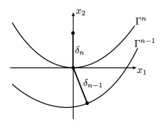
Figure 1: Motion of a single point of the interface in the normal direction．The point moves a distance $\delta_{n}$ at step $n.$ Without loss of generality, the direction of motion at the $n^{th}$ step is in the $x_{2}$ direction.

Denoting the average velocity within the time interval $[(n-1)\tau,n\tau]$ by $\bar{V}_{n}$, one has

$$\delta_{n}=\bar{V}_{n}\tau,\ \ \ \ \delta_{n-1}=\bar{V}_{n-1}\tau,$$

and hence equation (6) can be written:

$$\bar{V}_{n}\tau=\bar{V}_{n-1}\tau-(2\kappa_{n}-\kappa_{n-1})\tau^{2}+O(\tau^{3}).$$

Formally assuming $|\kappa_{n}-\kappa_{n-1}|<C\tau$ for some non-negative $C$, one obtains

$$\bar{V}_{n}\tau=\bar{V}_{n-1}\tau-\kappa_{n}\tau^{2}+O(\tau^{3}),$$ (7)

and hence

$$\dot{V}_{n}=-\kappa_{n}+O(\tau)\hskip 30.0pt\text{(as $\tau\rightarrow 0$)}.$$ (8)

The damping term in equation (2) can be included by prescribing the initial velocity of the wave equation to be $v_{0}(\bm{x})=d_{n}(\bm{x})$. This can be seen by expanding $d_{n}(\bm{x})$ in a Taylor series about $\bm{x}={\bf{0}}$ (see [2]):

$$d_{n}(x_{1},x_{2})=x_{2}+\dfrac{1}{2}\kappa_{n}x_{1}^{2}+\dfrac{1}{6}(\kappa_{n})_{x_{1}}x_{1}^{3}-\dfrac{1}{2}\kappa_{n}^{2}x_{1}^{2}x_{2}+O(|\bm{x}|^{4}),$$ (9)

and appealing to Poisson’s formula (4):

$$u_{v}(t,\bm{x})=\dfrac{1}{2\pi ct}\int_{B(\bm{x},ct)}\dfrac{-tv_{0}(\bm{y})}{\sqrt{c^{2}t^{2}-|\bm{y}-\bm{x}|^{2}}}d\bm{y}.$$ (10)

Making the change of variables:

$$\bm{y}-\bm{x} =ct\bm{z},$$ (11)

we note that

$$O(|\bm{y}|^{4})=O(t^{4})\hskip 30.0pt\text{(as $t\rightarrow 0$)}.$$ (12)

We thus investigate the contribution of the first four terms in the Taylor expansion, $u_{v}^{1},u_{v}^{2},u_{v}^{3},$ and $u_{v}^{4}$. We begin with the lowest order term:

$$u_{v}^{1}(t,\bm{x}) =\dfrac{1}{2\pi ct}\int_{B(\bm{x},ct)}\dfrac{-ty_{2}}{\sqrt{c^{2}t^{2}-|\bm{y}-\bm{x}|^{2}}}d\bm{y}$$

$$=\dfrac{-t}{2\pi ct}\int_{B(0,1)}\dfrac{ctz_{2}+x_{2}}{ct\sqrt{1-|\bm{z}|^{2}}}(ct)^{2}d\bm{z}.$$

Appealing to function parity we have:

$$\int_{B(0,1)}\dfrac{z_{2}}{\sqrt{1-|\bm{z}|^{2}}}d\bm{z}=0,$$

and it follows that

$$u_{v}^{1}(t,\bm{x}) =\dfrac{-t}{2\pi}\int_{B(0,1)}\dfrac{x_{2}}{\sqrt{1-|\bm{z}|^{2}}}d\bm{z}.$$

By making the change of variables:

$$z_{1}=r\text{cos}\theta,\hskip 15.0ptz_{2}=r\text{sin}\theta,$$ (13)

one arrives at

$$u_{v}^{1}(t,\bm{x}) =\dfrac{-tx_{2}}{2\pi}\int_{0}^{1}\int_{0}^{2\pi}\dfrac{1}{\sqrt{1-r^{2}}}rd\theta dr$$

$$=\dfrac{-tx_{2}}{2\pi}\int_{0}^{1}\dfrac{2\pi r}{\sqrt{1-r^{2}}}dr$$

$$=-tx_{2}\int_{0}^{1}\dfrac{r}{\sqrt{1-r^{2}}}dr.$$

Composite function integration yields

$$u_{v}^{1}(t,\bm{x}) =-tx_{2}\int_{0}^{1}(1-r^{2})^{-\frac{1}{2}}(-2r)\left(-\dfrac{1}{2}\right)dr=-tx_{2}.$$ (14)

We next consider the influence of the second term:

$$u_{v}^{2}(t,\bm{x}) =\dfrac{1}{2\pi ct}\int_{B(\bm{x},ct)}\dfrac{-\dfrac{1}{2}t\kappa_{n}y_{1}^{2}}{\sqrt{c^{2}t^{2}-|\bm{y}-\bm{x}|^{2}}}d\bm{y}$$

$$=\dfrac{-t\kappa_{n}}{4\pi ct}\int_{B(\bm{x},ct)}\dfrac{y_{1}^{2}}{\sqrt{c^{2}t^{2}-|\bm{y}-\bm{x}|^{2}}}d\bm{y}$$

$$=\dfrac{-t\kappa_{n}}{4\pi}\int_{B(0,1)}\dfrac{c^{2}t^{2}z_{1}^{2}+2ctx_{1}z_{1}+x_{1}^{2}}{\sqrt{1-|\bm{z}|^{2}}}d\bm{z}.$$

As before, function parity yields

$$\int_{B(0,1)}\dfrac{z_{1}}{\sqrt{1-|\bm{z}|^{2}}}d\bm{z}=0,$$

and hence

$$u_{v}^{2}(t,\bm{x}) =\dfrac{-t\kappa_{n}}{4\pi}\int_{B(0,1)}\dfrac{c^{2}t^{2}z_{1}^{2}+x_{1}^{2}}{\sqrt{1-|\bm{z}|^{2}}}d\bm{z}.$$

Making the change of variables (13), we have

$$u_{v}^{2}(t,\bm{x}) =\dfrac{-t\kappa_{n}}{4\pi}\int_{0}^{1}\int_{0}^{2\pi}\dfrac{c^{2}t^{2}r^{3}\text{cos}^{2}\theta+x_{1}^{2}r}{\sqrt{1-r^{2}}}d\theta dr$$

$$=\dfrac{-t\kappa_{n}}{4\pi}\int_{0}^{1}\int_{0}^{2\pi}\dfrac{c^{2}t^{2}r^{3}\dfrac{1+\text{cos}2\theta}{2}+x_{1}^{2}r}{\sqrt{1-r^{2}}}d\theta dr$$

$$=\dfrac{-t\kappa_{n}}{4\pi}\int_{0}^{1}\dfrac{\pi\left(c^{2}t^{2}r^{3}+2x_{1}^{2}r\right)}{\sqrt{1-r^{2}}}dr.$$

Using another change of variables:

$$r=\text{cos}\theta,$$ (15)

allows one to obtain:

$$u_{v}^{2}(t,\bm{x}) =\dfrac{-t\kappa_{n}}{4}\int_{0}^{\frac{\pi}{2}}\dfrac{c^{2}t^{2}\text{cos}^{3}\theta+2x_{1}^{2}\text{cos}\theta}{\sqrt{1-\text{cos}^{2}\theta}}\text{sin}\theta d\theta$$

$$=\dfrac{-t\kappa_{n}}{4}\int_{0}^{\frac{\pi}{2}}\left(c^{2}t^{2}\dfrac{\text{cos}3\theta+3\text{cos}\theta}{4}+2x_{1}^{2}\text{cos}\theta\right)d\theta$$

$$=\dfrac{-t\kappa_{n}}{4}\left(c^{2}t^{2}\left(-\dfrac{1}{12}+\dfrac{3}{4}\right)+2x_{1}^{2}\right)$$

$$=-t\kappa_{n}\left(\dfrac{c^{2}t^{2}}{6}+\dfrac{x_{1}^{2}}{2}\right).$$ (16)

The third term is similar:

$$u_{v}^{3}(t,\bm{x}) =\dfrac{1}{2\pi ct}\int_{B(\bm{x},ct)}\dfrac{-\dfrac{1}{6}t(\kappa_{n})_{x_{1}}y_{1}^{3}}{\sqrt{c^{2}t^{2}-|\bm{y}-\bm{x}|^{2}}}d\bm{y}$$

$$=\dfrac{-t(\kappa_{n})_{x_{1}}}{12\pi ct}\int_{B(\bm{x},ct)}\dfrac{y_{1}^{3}}{\sqrt{c^{2}t^{2}-|\bm{y}-\bm{x}|^{2}}}d\bm{y}$$

$$=\dfrac{-t(\kappa_{n})_{x_{1}}}{12\pi}\int_{B(0,1)}\dfrac{z_{1}^{3}+3c^{2}t^{2}x_{1}z_{1}^{2}+3ctx_{1}^{2}z_{1}+x_{1}^{3}}{\sqrt{1-|\bm{z}|^{2}}}d\bm{z}.$$

Again appealing to function parity:

$$\int_{B(0,1)}\dfrac{z_{1}^{3}}{\sqrt{1-|\bm{z}|^{2}}}d\bm{z}=0,$$

and therefore

$$u_{v}^{3}(t,\bm{x}) =\dfrac{-t(\kappa_{n})_{x_{1}}}{12\pi}\int_{B(0,1)}\dfrac{3c^{2}t^{2}x_{1}z_{1}^{2}+x_{1}^{3}}{\sqrt{1-|\bm{z}|^{2}}}d\bm{z}.$$

The change of variables  (13) gives

$$u_{v}^{3}(t,\bm{x}) =\dfrac{-t(\kappa_{n})_{x_{1}}}{12\pi}\int_{0}^{1}\int_{0}^{2\pi}\dfrac{3c^{2}t^{2}x_{1}r^{3}\text{cos}^{2}\theta+x_{1}^{3}r}{\sqrt{1-r^{2}}}d\theta dr$$

$$=\dfrac{-t(\kappa_{n})_{x_{1}}}{12\pi}\int_{0}^{1}\int_{0}^{2\pi}\dfrac{3c^{2}t^{2}x_{1}r^{3}\dfrac{1+\text{cos}2\theta}{2}+x_{1}^{3}r}{\sqrt{1-r^{2}}}d\theta dr$$

$$=\dfrac{-t(\kappa_{n})_{x_{1}}}{12\pi}\int_{0}^{1}\dfrac{\pi\left(3c^{2}t^{2}x_{1}r^{3}+2x_{1}^{3}r\right)}{\sqrt{1-r^{2}}}dr,$$

while (15) allows one to express:

$$u_{v}^{3}(t,\bm{x}) =\dfrac{-t(\kappa_{n})_{x_{1}}}{12}\int_{0}^{\frac{\pi}{2}}\dfrac{3c^{2}t^{2}x_{1}\text{cos}^{3}\theta+2x_{1}^{3}\text{cos}\theta}{\sqrt{1-\text{cos}^{2}\theta}}\text{sin}\theta d\theta$$

$$=\dfrac{-t(\kappa_{n})_{x_{1}}}{12}\int_{0}^{\frac{\pi}{2}}\left(3c^{2}t^{2}x_{1}\dfrac{\text{cos}3\theta+3\text{cos}\theta}{4}+2x_{1}^{3}\text{cos}\theta\right)d\theta$$

$$=\dfrac{-t(\kappa_{n})_{x_{1}}}{12}\left(3c^{2}t^{2}x_{1}\left(-\dfrac{1}{12}+\dfrac{3}{4}\right)+2x_{1}^{3}\right)$$

$$=\dfrac{-t(\kappa_{n})_{x_{1}}}{6}\left(c^{2}t^{2}x_{1}+x_{1}^{3}\right).$$ (17)

The final term follows the same approach:

$$u_{v}^{4}(t,\bm{x}) =\dfrac{1}{2\pi ct}\int_{B(\bm{x},ct)}\dfrac{\dfrac{1}{2}t\kappa_{n}^{2}y_{1}^{2}y_{2}}{\sqrt{c^{2}t^{2}-|\bm{y}-\bm{x}|^{2}}}d\bm{y}$$

$$=\dfrac{t\kappa_{n}^{2}}{4\pi ct}\int_{B(\bm{x},ct)}\dfrac{y_{1}^{2}y_{2}}{\sqrt{c^{2}t^{2}-|\bm{y}-\bm{x}|^{2}}}d\bm{y}$$

$$=\dfrac{t\kappa_{n}^{2}}{4\pi}\int_{B(0,1)}\dfrac{c^{3}t^{3}z_{1}^{2}z_{2}+c^{2}t^{2}x_{2}z_{1}^{2}+2c^{2}t^{2}x_{1}z_{1}z_{2}}{\sqrt{1-|\bm{z}|^{2}}}$$

$$+\dfrac{2ctx_{1}x_{2}z_{1}+ctx_{1}^{2}z_{2}+x_{1}^{2}x_{2}}{\sqrt{1-|\bm{z}|^{2}}}d\bm{z}.$$

Function parity tells us that

$$\int_{B(0,1)}\dfrac{z_{1}^{2}z_{2}}{\sqrt{1-|\bm{z}|^{2}}}d\bm{z}=0,$$

and hence

$$u_{v}^{4}(t,\bm{x}) =\dfrac{t\kappa_{n}^{2}}{4\pi}\int_{B(0,1)}\dfrac{c^{2}t^{2}x_{2}z_{1}^{2}+2c^{2}t^{2}x_{1}z_{1}z_{2}+x_{1}^{2}x_{2}}{\sqrt{1-|\bm{z}|^{2}}}d\bm{z}.$$

Applying the change of variables (13) and computing gives

$$u_{v}^{4}(t,\bm{x}) =\dfrac{t\kappa_{n}^{2}}{4\pi}\int_{0}^{1}\int_{0}^{2\pi}\dfrac{c^{2}t^{2}x_{2}r^{3}\text{cos}^{2}\theta+2c^{2}t^{2}x_{1}r^{3}\text{cos}\theta\text{sin}\theta+x_{1}^{2}x_{2}r}{\sqrt{1-r^{2}}}d\theta dr$$

$$=\dfrac{t\kappa_{n}^{2}}{4\pi}\int_{0}^{1}\int_{0}^{2\pi}\dfrac{c^{2}t^{2}x_{2}r^{3}\dfrac{1+\text{cos}2\theta}{2}+c^{2}t^{2}x_{1}r^{3}\text{sin}2\theta+x_{1}^{2}x_{2}r}{\sqrt{1-r^{2}}}d\theta dr$$

$$=\dfrac{t\kappa_{n}^{2}}{4\pi}\int_{0}^{1}\dfrac{\pi\left(c^{2}t^{2}x_{2}r^{3}+2x_{1}^{2}x_{2}r\right)}{\sqrt{1-r^{2}}}dr.$$

Using the change of variables (15) leads us to the expession:

$$=\dfrac{t\kappa_{n}^{2}}{4}\int_{0}^{\frac{\pi}{2}}\dfrac{c^{2}t^{2}x_{2}\text{cos}^{3}\theta+2x_{1}^{2}x_{2}\text{cos}\theta}{\sqrt{1-\text{cos}^{2}\theta}}\text{sin}\theta d\theta$$

$$=\dfrac{t\kappa_{n}^{2}}{4}\int_{0}^{\frac{\pi}{2}}\left(c^{2}t^{2}x_{2}\dfrac{\text{cos}3\theta+3\text{cos}\theta}{4}+2x_{1}^{2}x_{2}\text{cos}\theta\right)d\theta$$

$$=\dfrac{t\kappa_{n}^{2}}{4}\left(c^{2}t^{2}x_{2}\left(-\dfrac{1}{12}+\dfrac{3}{4}\right)+2x_{1}^{2}x_{2}\right)$$

$$=t\kappa_{n}^{2}\left(\dfrac{c^{2}t^{2}x_{2}}{6}+\dfrac{x_{1}^{2}x_{2}}{2}\right).$$ (18)

Equations (14)，(16)，(17)，and (18) together express

$$u_{v}(t,\bm{x})= -t\left(x_{2}+\kappa_{n}\left(\dfrac{c^{2}t^{2}}{6}+\dfrac{x_{1}^{2}}{2}\right)+\dfrac{(\kappa_{n})_{x_{1}}}{6}\left(c^{2}t^{2}x_{1}+x_{1}^{3}\right)\right)$$ (19)

$$+t\kappa_{n}^{2}\left(\dfrac{c^{2}t^{2}x_{2}}{6}+\dfrac{x_{1}^{2}x_{2}}{2}\right).$$

Upon taking $t=\tau$ and $\bm{x}=(0,\delta_{n})$, we arrive at

$$0 =-\tau\left(\delta_{n}+\kappa_{n}\dfrac{c^{2}\tau^{2}}{6}-\kappa_{n}^{2}\dfrac{c^{2}\tau^{2}\delta_{n}}{6}\right)=-\delta_{n}\tau+O(\tau^{3}).$$ (20)

Combining this equation with our previous results yields:

$$\delta_{n}-\delta_{n-1}-\delta_{n}\tau=-(2\kappa_{n}-\kappa_{n-1})\tau^{2}+O(\tau^{3}).$$ (21)

Writing $\delta_{n}=\bar{V}_{n}\tau$ and $\delta_{n-1}=\bar{V}_{n-1}\tau$ in equation (21) expresses

$$\bar{V}_{n}\tau-\bar{V}_{n-1}\tau-\bar{V}_{n}\tau^{2}=-(2\kappa_{n}-\kappa_{n-1})\tau^{2}+O(\tau^{3}).$$

Formally assuming $|\kappa_{n}-\kappa_{n-1}|<C\tau$, for some constant $C$, and dividing both sides by $\tau^{2}$ gives

$$\dfrac{\bar{V}_{n}-\bar{V}_{n-1}}{\tau}-\bar{V}_{n}=-\kappa_{n}+O(\tau).$$

It follows that the damping term enters the equation of motion:

$$\dot{V}_{n}-V_{n}=-\kappa_{n}+O(\tau).$$ (22)

By linearity, taking $u_{0}(\bm{x})=a(2d_{n}(\bm{x})-d_{n-1}(\bm{x}))$ and $v_{0}(\bm{x})=bd_{n}(\bm{x})$ one can obtain the interfacial motion:

$$a\dot{V}_{n}-bV_{n}=-\dfrac{ac^{2}}{2}\kappa_{n}+O(\tau),$$ (23)

where $a$ and $b$ are real parameters. Therefore, one can rewrite the parameters:

$$\alpha=a,\hskip 15.0pt\beta=-b,\hskip 15.0pt\gamma=\dfrac{ac^{2}}{2},$$ (24)

to approximate a prescribed interfacial motion:

$$\alpha\dot{V}+\beta V=-\gamma\kappa+O(\tau).$$ (25)

The previous results show that the wave equation’s initial velocity can be used in the HMBO algorithm to impart damping terms. In the next section, by choosing parameters, we will make a numerical investigation into using the HMBO to approximate interfacial motion by the standard mean curvature flow.

3 The HMBO approximation of mean curvature flow

An approximation method for mean curvature flow can be obtained by returning to equation (4) and choosing appropriate initial conditions. For a predetermined time step $\tau>0$, we take $u_{0}(\bm{x})=0$, $v_{0}(\bm{x})=d_{n}(\bm{x})$, and $c^{2}=\lambda/\tau$. Then equation (20) gives

$$0 =-\tau\left(\delta_{n}+\kappa_{n}\dfrac{\lambda\tau}{6}-\kappa_{n}^{2}\dfrac{\lambda\delta_{n}\tau}{6}\right)+O(\tau^{3}),$$

$$=\delta_{n}+\kappa_{n}\dfrac{\lambda\tau}{6}-\kappa_{n}^{2}\dfrac{\lambda\delta_{n}\tau}{6}+O(\tau^{2}).$$

Preceeding as in the previous section, we obtain

$$\bar{V}_{n}=-\dfrac{\lambda}{6}\kappa_{n}+O(\tau).$$

Since $\lambda$ is a free parameter, we find that the corresponding threshold dynamics can approximate curvature flow with a parameter $\gamma$:

$$V_{n}=-\gamma\kappa_{n}+O(\tau)\hskip 30.0pt(\text{as $\tau\rightarrow 0$}).$$ (26)

4 Numerical investigation

We will now perform a numerical error analysis of the HMBO approximation of MCF. The numerical method’s performance will be compared to the case of a circle evolving by MCF. In such a setting, the evolution of the circle’s radius is governed by the solution of the following ordinary differential equation:

$$\begin{cases}\dot{r}(t)=-\dfrac{1}{r(t)}\ \ \ \ t>0,\\ r(0)=r_{0},\end{cases}$$ (27)

where $r_{0}$ is the initial radius of the circle. We remark that the radius decreases until its extinction time $t_{e}=r_{0}^{2}/2$, and that $r(t)=\sqrt{r_{0}^{2}-2t}$.

The HMBO approximation method solves the following wave equation for a small time $\tau>0$:

$$\begin{cases}u_{tt}=c^{2}\Delta u\ &\text{in}\ (0,\tau)\times\Omega\\ u(0,\bm{x})=0\ &\text{in}\ \Omega\\ u_{t}(0,\bm{x})=d_{k}(\bm{x})\ &\text{in}\ \Omega\\ \partial_{\bm{n}}u=0\ &\text{on}\ \partial\Omega,\end{cases}$$ (28)

where $\Omega=(-2,2)\times(-2,2)$ and $k$ denotes the $k^{th}$ step of the HMBO algorithm. We choose the initial interface to be a circle with radius one, so that

$$d_{0}(\bm{x})=||\bm{x}||-1.$$

The initial velocity at the $k^{th}$ step is then defined as the signed distance function to the zero level set of the solution to the wave equation:

$$d_{k}(\bm{x})=\begin{cases}\inf_{\bm{y}\in\partial\{u(\bm{x},\tau)>0\}}||\bm{x}-\bm{y}||\hskip 30.0pt\bm{x}\in\{u(\bm{x},\tau)>0\}\\ -\inf_{\bm{y}\in\partial\{u(\bm{x},\tau)>0\}}||\bm{x}-\bm{y}||\hskip 21.0pt\text{otherwise.}\end{cases}$$ (29)

Since the extinction time $t_{e}$ depends on $r_{0}$, we set $\tau=t_{e}/N_{\tau}$. Here $r_{0}=1$ (hence $t_{e}=0.5$), and we set $N_{\tau}=150$ to ensure a level of precision. The time step is then $\tau=3.33\times 10^{-3}$. The target problem (27) corresponds to $\gamma=1$ in equation (26), and we thus set $c^{2}=6/\tau$.

Finite differences are used to numerically solve the wave equation with a time step $\Delta t=2.22\times 10^{-6}$. The grid spacing in the $x$ and $y$ directions are equal to $\Delta x=2/(N-1)$, where $N$ is a natural number. We examine the numerical error when $N=2^{j},$ for $j=4,5,6,7,8$. The numerical results are shown in figure 2, where the radius of the numerical solution is defined to be the average distance $\tilde{r}(t)$ of the level set’s point cloud to the origin.

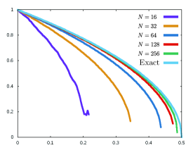
Figure 2: Convergence of the approximation method as $N$ is increased.

The error is measured using the quantity:

$$Err(t)=\int_{0}^{T}|r(t)-\tilde{r}(t)|dt.$$ (30)

Since the extinction time of the numerical solution differs from the exact solution, the actual error is computed as follows:

$$Err(t)\approx\displaystyle\sum_{i=0}^{N_{s}}|r(i\tau)-\tilde{r}(i\tau)|\tau,$$ (31)

where $N_{s}$ denotes the number of time steps until the numerical solution’s radius disappears (the corresponding time is $N_{s}\tau$). Our results are summarized in table (31), where we observe the convergence of our method to the exact solution.

Table 1: Error Table with respect to $\Delta x.$

$N$	$N_{s}\tau$	$Err$
16	0.223333	0.044613
32	0.343333	0.039463
64	0.436667	0.022746
128	0.473333	0.008509
256	0.486667	0.003907

5 Acknowledgments

E. Ginder would like to acknowledge the support of JSPS Kakenhi Grant Number 17K14229, as well as that from the Presto Research Program of the Japan Science and Technology Agency.

References

[1] Y. G. Chen, Y. Giga, and S. Goto. “Uniqueness and existence of viscosity solutions of generalized mean curvature flow equations” Journal of Differential Geometry, Vol. 33, Number 3 (1991), 749-786.
[2] S. Essedoglu, S. Ruuth, R. Tsai. “Diffusion generated motion using signed distance functions” J. Comp. Phys., 229, 4 (2010), 1017-1042.
[3] E. Ginder, K. Svadlenka. “Wave-type threshold dynamics and the hyperbolic mean curvature flow” Japan Journal of Industrial Applied Mathematics, doi 10.1007/s13160-016-0221-0, (2016).
[4] P. G. LeFloch, K. Smoczyk. “The hyperbolic mean curvature flow” Journal de Mathmatiques Pures et Appliques, Vol. 90, Issue 6 (2008), 591-614.
[5] B. Merriman, J. Bence, S. Osher. “Diffusion Generated Motion by Mean Curvature” UCLA CAM, (1992), 1-11.
[6] S. Osher, R. Fedkiw. “Level Set Methods and Dynamic Implicit Surfaces” Applied Mathematical Science, (2003).
[7] R. C. Reilly. “Mean Curvature, The Laplacian, and Soap Bubbles” The American Mathematical Monthly, Vol. 89, No. 3 (1982), 180-188.
[8] S. Shin, D. Juric. “High Order Level Contour Reconstruction Method” Journal of Mechanical Science and Technology, Vol. 21, (2007), 311-326.