A Geometrical Branch-and-Price (GEOM-BP) Algorithm for Big Bin Packing Problems

Abstract

Bin packing problem examines the minimum number of identical bins needed to pack a set of items of various weights. This problem arises in various areas of the artificial intelligence demanding derivation of the exact solutions in the shortest amount of time. Employing branch-and-bound and column generation techniques to derive the exact solutions to this problem, usually requires designation of problem-specific branching rules compatible with the nature of the polluted pricing sub-problem of column generation. In this work, we present a new approach to deal with the forbidden bins which handles two-dimensional knapsack problems. Furthermore, a set of diving criteria are introduced which emphasize the importance of the geometrical features of the bins. It is further shown that efficiency of the column generation technique could significantly get improved using an implicit sectional pricing scheme. The proposed algorithm outperforms the current state-of-the-art algorithms in number of the benchmark instances solved in less than one minute.

1 Introduction

In a bin packing problem (BPP), we are given an unlimited number of bins of identical capacity $c>0$ and a set of items $I=\{i_{1},\dots,i_{n}\}$ each of which having a weight $w_{i}$ $(0<w_{i}\leq c)$, and the goal is to pack all the items in a minimum number of bins without exceeding bins’ capacities. For practical problems, we can assume that the weights and capacities are integers.

The BPP arises in various areas of the artificial intelligence including cloud resource allocation and management [1, 2, 3, 4, 5], automatic power plant assignments [6, 7] and multimedia processing [7, 8]. In many of these applications, the exact solutions to the problem are often required to be obtained.

To the best of our knowledge, the most recent review on exact algorithms used for solving BPP is presented by Delorme et al. [9, 10] where the authors have reviewed various formulations of BPP and conducted extensive experiments on benchmark instances. Broadly speaking, the develped exact algorithms fall into one of the following categories: branch-and-bound [11, 12, 13], branch-and-price [14, 15, 16, 17, 18, 19] and pseudo-polynomial algorithms [20, 21, 22, 23, 24, 25].

In this paper, we present an exact algorithm for solving the BPP and that relies on branch-and-bound and column generation techniques. Employing column generation in a branch-and-bound tree (also known as branch-and-price algorithm), requires the development of rigorous methods to solve the pricing sub-problem of the column generation. Specifically, when branching occurs on variables of the Gilmore-Gomory model [26, 27], bins known as the forbidden bins (patterns) are dealt with while proceeding into the depth of the branch-and-bound tree. The forbidden bins should then be systematically excluded from the search domain of the one-dimensional knapsack problem (1D-KSP).

To address the issue of having a polluted pricing sub-problem in column generation, two main approaches have been introduced in the literature. The first approach determines the $K$-best solutions of the 1D-KSP at the $(k-1)$-th level of the tree. This guarantees that enough number of bins is available to be added to the restricted master problem in case all bins appear to be forbidden ones during column generation. Although some attempts (see [28, 29]) have been made to determine the $K$-best solutions of the 1D- KSP, there still persists a lack of methods featuring universal applicability. In the second approach, a set of branching rules is designed that avoids emergence of forbidden bins in the pricing sub-problem of column generation [15, 16, 17, 19]. The drawbacks of such branching schemes have been discussed in details by Vanderbeck [30].

As an alternative, a new approach to deal with forbidden bins is proposed in this work. A constraint referred to as a decrement constraint is added to the 1D-KSP whenever one of the forbidden bins is met during column generation. This extra constraint compels the pricing sub-problem to generate the next feasible solution of the 1D-KSP. Subsequently, the generated solution (bin) is passed to the restricted master problem. Premature termination of column generation might occur when employing our proposed method. The consequences of such an undesired termination on the branch-and-price algorithm are investigated and resolved in this paper.

Another important aspect of efficient branch-and-price algorithms has to do with primal heuristics. A thorough study of different primal heuristics like diving, relaxation induced neighborhood search and local branching has been reported earlier [31]. Yet, the importance of the geometrical features of bins (such as Pythagorean means of weights of the items packed into bins) in diving methods has not received any attention in the literature. In this work, we further exploit the geometrical features of bins in enhancing performance of the diving methods and propose an effective primal heuristic that is called batch diving. Our concern, like in other primal heuristics, is to take full advantage of LP relaxation solutions for constructing the integer solutions. Batch diving is in fact a multi-dimensional knapsack problem that plays a key role in accelerating the proposed geometrical branch-and-price (GEOM-BP) algorithm.

In Sect. 2, the set partitioning formulation of the BPP, column generation and implicit sectional pricing scheme are presented. In this section, a simple method named subset-sum-$\tilde{n}$ heuristic used to initialize column generation is also proposed. Geometrical interpretations of packing problems and their use in enhancing the diving methods is addressed in Sect. 3. The mathematical model that considers batch diving as a generalization of geometrical diving methods is described in Sect. 4. In Sect. 5, we present a branching scheme that divides the search region of a problem in a way that exploration of the nodes with forbidden bins becomes an indispensable aspect of the Geom-BP algorithm. Finally, computational results and discussions are presented in Sect. 7.

2 Mathematical Formulation

A BPP as defined earlier could be considered as a special case of one-dimensional cutting stock problem (1D-CSP). In 1D-CSP, each item is further associated with a demand $d_{i}$ $(d_{i}\in Z^{+})$. The set of items $I=\{i_{1},\dots,i_{n}\}$ will then contain items with unique weights only, and the items accommodated into bins of the solutions should further satisfy their corresponding demands.

It is noteworthy that in the context of the CSP, bins are usually referred to as cutting rolls, cutting patterns or simply patterns with the latter appellation being the most frequent in the literature. Also, when column generation technique is involved, the terms column, bin and pattern are used synonymously.

Even though modeling and solving either of the BPP or 1D-CSP yields optimal number of bins, 1D-CSP formulation is preferred when iterative matrix-based algorithms like column generation are used in the solving procedure. This is due to the dimensions of the matrices that are lower when the cutting stock approach is adopted, considering the fact that the majority of BPP instances from industry as well as the ones found in the literature involve items with same weights. For the purpose of this work, the classical definition of BPP given in Sect. 1 is altered to include demands as extra attributes of items in addition to their weights.

2.1 Set Partitioning Formulation and Column Generation

Set partitioning formulation for BPP is introduced as

$$\min \ \sum_{k=1}^{K}\lambda_{k}$$ (1a)

$$\mathrm{s.t.} \ \sum_{k=1}^{K}x_{ik}\lambda_{k}=d_{i} \quad i=1,\dots,n$$ (1b)

$$\ \lambda_{k}\geq{0}\ \mathrm{and\ integer} \quad k=1,\dots,K\ ,$$ (1c)

where $\lambda_{k}$ is the load of bin $k$ (number of times bin $k$ is used), and $K$ denotes an upper bound on the number of possible bins. The variable $x_{ik}$ in (1b) is the number of replications of item $i$ in bin $k$, and this set of constraints ensures that all the items satisfy their demands. Also, feasibility of the bins are ensured by the constraint

$$\left\{\sum_{i=1}^{n}w_{i}x_{ik}\leq c\ ,\ k=1,\dots,K\ ,\ x_{ik}\in\{0,\dots,d_{i}\}\ ,\ i=1,\dots,n\right\}\ .$$ (2)

To solve the LP relaxation of model (1), it is impractical to enumerate all the possible bins, a fact that calls for column generation technique. By dropping the integrality constraint in (1b), the master problem for the BPP is derived as

$$\min \ \sum_{k=1}^{K}\lambda_{k}$$ (3a)

$$\mathrm{s.t.} \ \sum_{k=1}^{K}x_{ik}\lambda_{k}=d_{i} \quad i=1,\dots,n$$ (3b)

$$\ \lambda_{k}\geq{0} \quad k=1,\dots,K\ .$$ (3c)

Solving model (3) using column generation starts by first defining the restricted master problem (RMP) initialized by a basic feasible solution. The RMP is then solved to optimality by the revised simplex method and its dual prices denoted by $\boldsymbol{\pi}$, are assumed to be the cost coefficients of the pricing sub-problem

$$\nu_{\mathrm{exact}}(\boldsymbol{\pi})=\max\left\{\sum_{i=1}^{n}\pi_{i}x_{i}-1:\sum_{i=1}^{n}w_{i}x_{i}\leq c\ ,\ x_{i}\in\{0,\dots,d_{i}\}\ ,\ i=1,\dots,n\right\}\ ,$$ (4)

and the generated bin by solving the 1D-KSP (4) is subsequently added to the RMP. A given bin terminates the column generation process in case its reduced cost $\nu_{\mathrm{exact}}(\boldsymbol{\pi})\leq 0$. Were it to be the case, termination of column generation indicates that all of the bins with positive reduced costs have been priced out.

It is pointed out that the method used for solving the pricing sub-problem (4) should be capable of finding the exact solution of the 1D-KSP problem upon termination of column generation. Otherwise, column generation could be terminated prematurely. In this case, the objective value of the master problem solved at the root node of the tree would not represent a lower bound on the BPP.

2.2 Implicit Sectional Pricing Scheme

There are two major factors contributing to the amount of computational time when master problem is solved by column generation: i) the dimensions of the basis of the master problem, ii) the dimensions of the pricing sub-problem. The dimensions of the basis determine the performance of basis- updating techniques. This is due to the fact that most of the computational time needed for column generation technique elapses while updating the basis. On the other hand, dimensions of the pricing sub-problem determine how fast the new columns (bins) are generated during column generation.

Dimensions of the pricing sub-problem could be reduced through solving a binary 1D-KSP

$$\nu_{\mathrm{sec}}(\boldsymbol{\pi})=\max\left\{\sum_{i=1}^{n}\pi_{i}x_{i}-1:\sum_{i=1}^{n}w_{i}x_{i}\leq c\ ,\ x_{i}\in\{0,1\}\ ,\ i=1,\dots,n\right\}\ ,$$ (5)

where the generated columns contain unique items (no items with same weights). This set of columns form a section implicitly and our computational experiments show that picking the entering column from the defined implicit section (5) is efficient. However, there are other columns not defined by (5). For this reason, whenever a column generated by solving model (5) is priced out with negative reduced cost, the original pricing sub-problem (4) is called to prove optimality of the column generation.

2.3 Subset-sum-$\tilde{n}$ Heuristic

Quiroz-Castellanos et al. [32] propose a first fit algorithm with $\tilde{n}$ pre-allocated-items (FF-$\tilde{n}$) to be used as an upper bounding technique for BPP. In FF-$\tilde{n}$, the items $\tilde{N}=\left\{i\in I:w_{i}\geq\lceil{\frac{c}{2}}\rceil\right\}$ are placed into separate bins, then the first fit algorithm is ran to place the remaining items into the bins.

In our proposed subset-sum-$\tilde{n}$ heuristic, the $\tilde{n}$ large items $(\tilde{n}=|\tilde{N}|)$, similarly to FF-$\tilde{n}$, are accommodated into separate bins. Subsequently, instead of using the first fit algorithm, the 1D-KSP

$$\max\left\{\sum_{i=1}^{n}w_{i}x_{i}:\sum_{i=1}^{n}w_{i}x_{i}\leq c\ ,\ x_{i}\in\{0,\dots,d_{i}\}\ ,\ i=1,\dots,n\right\}\ ,$$ (6)

also known as the subset-sum problem is employed and solved iteratively until all the remaining items are assigned to bins. The objective of model (6) is to maximize the fill of the bins. Such well-filled bins could effectively be used as good candidates to initialize column generation.

3 Geometrical Diving

In diving methods, branching usually occurs on a bin with the highest value in the solution of master problem and is followed by re-optimization of the residual problem [30, 33]. This process is continued at each node until an integer solution referred to as primal heuristic solution is achieved.

In this work, the diving criteria are formulated using the Lehmer mean of the weights of items packed into the bins. Recall that, for a given set of weights $W=\{w_{j}:w_{j}\in\mathbb{R}\ ,\ j=1,2,\dots,J\}$, the Lehmer mean function $L_{p}(W)$ is defined as

$$L_{p}(W)=\dfrac{\sum\limits_{j=1}^{J}w_{j}^{p}}{\sum\limits_{j=1}^{J}w_{j}^{p-1}}\ ,$$ (7)

for every $p\in\mathbb{R}$ [34]. Special Lehmer means are obtained when values of $p$ are set to $0$ and $2$, where the terms $L_{0}(W)$ and $L_{2}(W$) are known as the harmonic and contra-harmonic means of the set $W$, respectively.

Obtaining a solution to BPP by packing the larger items first, could then be modeled by considering the contra-harmonic mean of the bins as diving criterion. This is due to the fact that small items make small contributions to the contra-harmonic mean of their containing bins. Among all the bins obtained by solving the master problem at each node, the bin having the maximum contra-harmonic mean could potentially be selected for diving. Similarly, when shifting priority to the small items, harmonic means of the bins could potentially be considered as the diving criterion.

An alternative diving criterion could further be obtained by considering different Lehmer means simultaneously. The criterion

$$L_{s}=\int_{0}^{2}pL_{p}(W)dp\ ,$$ (8)

assumes different Lehmer means ranging from harmonic to contra-harmonic means where the impacts of the smaller items are relaxed by applying the multiplier $p$. The following example illustrates an application of the geometrical diving criteria.

Example 1

Let $n=6$, $c=100$, $I=\{1,2,3,4,5,6\}$, $W_{I}=\{72,54,34,33,19,18\}$ and $D_{I}=\{1,1,1,1,1,1\}$. Solving the master problem at the root node, yields the following set of bins

$$B_{\mathrm{rel}}=\left\{\{i_{1},i_{5}\},\{i_{2},i_{3}\},\{i_{3},i_{4},i_{6}\},\{i_{2},i_{4}\},\{i_{2},i_{5},i_{6}\},\{i_{1},i_{6}\}\right\}\ ,$$

where the relaxed values bins are obtained as being $0.8,0.4,0.6,0.4,0.2$ and $0.2$, respectively. By setting the diving criterion to be the highest-value, diving at the root node occurs on $B_{1}=\{i_{1},i_{5}\}$. However, by setting the criterion to be $L_{0}$ , $B_{2}=\{i_{2},i_{3}\}$ gets selected whose small item is larger than the small items contained in the other bins. On the other hand, the criterion $L_{2}$ selects $B_{6}=\{i_{1},i_{6}\}$ where the larger item $i_{1}$ is prioritized. Furthermore, by evaluating the integral (8) for each bin, $B_{1}$ gets selected as the candidate for diving.

For this simple example, employing any of the geometrical diving criteria leads to the primal heuristic solution having the optimal number of bins. Composition of the items into bins in $B_{\mathrm{rel}}$ and the corresponding harmonic and contra-harmonic means for each bin are depicted in Fig. 1.

4 Batch Diving

Practically speaking, the diving methods described in Sect. 3 could not be implemented efficiently since the computational time for re-optimization of the child nodes remain close to the computational time of their parent nodes. For this reason, a batch diving procedure is proposed where diving occurs on a batch of bins concurrently.

Let us assume that $\bar{n}$ items are present in a certain node ($\bar{n}=n$ at the root node) and let $\bar{d}_{i}$ denote the corresponding residual demand of each item, where $i=1,\dots,\bar{n}$. The model for batch diving is introduced as

$$\min \ \sum_{k=1}^{K^{\star}}\gamma_{k}\mu_{k}$$ (9a)

$$\mathrm{s.t.} \ \sum_{k=1}^{K^{\star}}x_{ik}\mu_{k}=\bar{d}_{i} \quad i=1,\dots,\bar{n}$$ (9b)

$$\ \mu_{k}\in\{0,1\} \quad k=1,\dots,K^{\star}\ ,$$ (9c)

where $K^{\star}$ is the number of bins obtained when master problem is solved at the considered node. Solving (9) returns a set of high quality bins, with respect to the diving criterion. In (9a), $\gamma_{k}$ is the value of the diving criterion for bin $k$ and $\mu_{k}$ is the load of bin $k$, where $\mu_{k}=1$ if the $k$-th bin is present in the set of bins candidate for batch diving, $0$ otherwise. Also, the set of constraints (9b) ensure that diving on a batch of some selected bins would not lead to an infeasible node.

After batch diving is performed at each node, dimensions of the residual problem decrease significantly, which in turn would speed up the re-optimization process. It is also possible to perform the batch diving on smaller subsets of bins at each node in order to increases the chances of constructing the optimal solution to BPP.

5 Polluted Pricing Sub-problem

The branching rule in the GEOM-BP algorithm is the very same criterion used in diving, and more attention is put on forbidden bins by exploring the tree in a binary manner. As a consequence, a single bin is added either to the partial upper bound solution or to the list of the forbidden bins. In the binary, compared to the integer branching strategy, more nodes containing forbidden bins are explored. It is worth mentioning that the paths to optimal solutions of some of the most difficult instances of BPP are likely to be the ones that visit the polluted nodes.

As mentioned earlier, the main concern in developing branch-and-price algorithms pertains to overcoming the issue of the presence of forbidden bins polluting the search space of the pricing sub-problem. Our approach when dealing with the polluted pricing sub-problem of column generation is straightforward. In practice, whenever one of the forbidden bins is met, a two-dimensional knapsack problem (2D-KSP) is solved in order to derive the next feasible solution to the pricing sub-problem. Assume that a forbidden bin is generated at the $k$-th iteration of column generation with an objective value $\nu_{k}$ where

$$\nu_{k}=\sum\limits_{i=1}^{n}\pi_{i}x_{i}-1\ ,$$ (10)

then the next feasible solution to the pricing sub-problem could be obtained by solving

$$\nu_{\mathrm{2D-KSP}}(\boldsymbol{\pi})=\max \ \sum_{i=1}^{n}\pi_{i}x_{i}-1$$ (11a)

$$\mathrm{s.t.} \ \sum_{i=1}^{n}\pi_{i}x_{i}\leq c$$ (11b)

$$\ \sum_{i=1}^{n}\pi_{i}x_{i}-1\leq\nu_{k}-\delta$$ (11c)

$$\ x_{i}\in\{0,1,\dots,\bar{d}_{i}\} \quad i=1,\dots,\bar{n}\ ,$$ (11d)

where $\delta$ denotes the value of a decrement. In this model, (11c) is referred to as the decrement constraint, and it ensures that the generated bin will have an objective value lower than $\nu_{k}$. In other words, (11) guarantees that an arbitrary generated bin contains a composition of items different from that of the forbidden one. The process is repeated in case the generated bin after solving (11) appears to be one of the other forbidden bins again.

An important aspect of (11) is the value assigned to the decrement. For large values of $\delta$, there could emerge possibilities to skip some high quality solutions of the sub-problem. More importantly, the bin generated by this model could cause termination of column generation. In such a case, since solving (11) does not guarantee the achievement of the second best solution of the sub-problem, column generation might terminate prematurely.

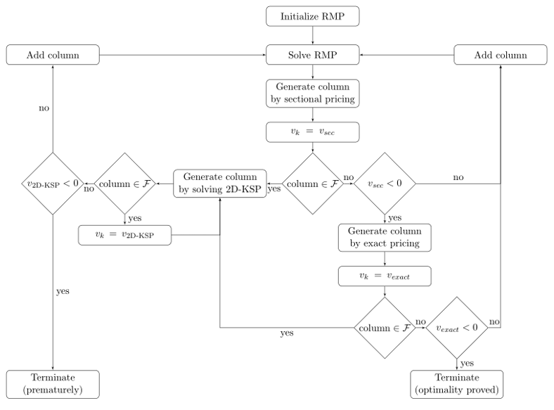
Figure 2: Schematic of steps for solving master problems in GEOM-BP.

It is noted that even when considering a minimal decrement, achievement of the second best solution is not guaranteed. For these nodes, pruning by bound is not allowed and branching is resumed. Usually, by considering sufficiently small values for the decrement $\delta$, optimality of the column generation gets successfully proved for the majority of the nodes. Figure 2 depicts an schematic of the steps described above where $\mathcal{F}$ denotes the set of forbidden bins.

6 Computational Results

In this section, we present computational results for running the GEOM-BP algorithm on the benchmark instances. Armadillo C++ [35] library was used as the main hub for programming, and the C codes for COMBO [36] and BOUKNAP [37] were compiled in GCC 7.2.0 to solve the binary and bounded 1D-KSP, respectively. Furthermore, the 2D-KSP were solved calling the Fortran sub-routine provided by Martello et al. [38], and the multi-dimensional knapsack problems arising in the batch diving models were solved employing CPLEX 12.7.0 . All experiments were carried out on an Intel core i-7 6700 HQ 2.6 GHz with 16 GB RAM, but only a single core was allowed when executing the algorithms to have a reasonable comparison with other methods.

The classes of benchmark instances considered in this work include:

• A set of 80 instances ‘Falkenauer U’ and a set of 80 triplets ‘Falkenauer T’ presented by Falkenauer in [39].

• Sets of 720 instances ‘Scholl 1’, 480 instances ‘Scholl 2’ and 10 instances ‘Scholl 3’ presented by Scholl et al. in [12].

• A set of 17 instances ‘Wäscher’ presented by Wäscher and Gau in [40].

• Sets of 100 instances ‘Schwerin 1’ and 100 instances ‘Schwerin 2’ presented by Schwerin and Wäscher in [41].

• A set of 28 instances ‘Hard28’ presented by Schoenfield in [42].

• A set of 3840 instances ‘Delorme R’ presented by Delorme et al. in [9].

However, the trivial instances from the literature whose computed combinatorial lower bounds coincide with the number of bins resulting from the Best Fit Decreasing algorithm were excluded from experiments. The combinatorial lower bound for each instance could be computed by a method presented by Martello and Toth [11].

Table 1 compares the results obtained using GEOM-BP to the exact algorithms from the literature, namely MTP[11], BISON [12], ONECUT [21], ARCFLOW [23], VPSOLVER [25], VANCE [15] and BELOV [14]. We adapt the computational results reported by Delorme et al. [9] as the bechmark. It is observed that Geom-BP algorithm, using any of the introduced geometrical criteria $L_{0}$, $L_{2}$ or $L_{s}$ outperforms the previously developed exact algorithms in the tested number of instances solved in less than one minute.

It is noteworthy to mention that GEOM-BP shows a significant improvement over BELOV algorithm when solving the instances of class ‘Falkenauer T’. This is mainly due to the fact that these instances hold Round-Up Property (RUP) where the objective value of the master problem solved at the root node is equal to the optimal number of bins, and the use of our proposed heuristic together with the batch diving procedure prove useful in constructing the optimal bins as fast as possible.

For the more challenging instances of class ‘Hard28’, BELOV algorithm remains superior both in the number of instances solved in less than one minute and the average computational time. This class contains $5$ instances with Non-Integer Round-Up Property (Non-IRUP) where the gap between the integer solution and the LP relaxation at the root node is greater than or equal to $1$. For these Non-IRUP instances, the gaps are not closed and GEOM-BP proves the optimality of the solutions by exploring and exhausting all the possible nodes. It is pointed out that an appropriate choice for the decrement value $\delta$ in (11) leads to termination of branch-and-price algorithm in less than one minute. In this work, we use an adaptive scheme to determine the decrement value whose initial point is considered to be the relatively small value $\delta_{0}=10^{-5}$. For 2 instances from the ‘Hard28’ class, namely ‘BPP60’ and ‘BPP181’, optimality of the solutions were proved only by increasing the time limit to $10$ minutes. However, GEOM-BP could not close the gap for the instance ‘BPP40’ in less than $10$ minutes, and this instance remained unsolved.

For the ‘Scholl 3’ instances, the bottleneck for solving the master problem at the root node pertains to the large dimenstions of the sub-problems, preventing the competitive algorithms like VPSOLVER and BELOV from solving the instances efficiently. The sectional pricing scheme proposed in this work, leads GEOM-BP to solve these instances in shorter amounts of time by reducing the dimensions of the pricing sub-problems.

Further details for GEOM-BP are presented in Table (2). For each class of instances, the average total number of nodes explored ($n_{\mathrm{total}}^{\mathrm{node}}$) and the average total number of polluted nodes explored ($n_{\mathrm{poll}}^{\mathrm{node}}$) are reported. It is seen that for majority of the instances, the optimal solution is obtained without exploring the polluted nodes. However, for more difficult classes of ‘Falkenauer T’, ‘Wäscher’ and ‘Hard28’, optimal solutions are achieved only when the polluted nodes are explored. Furthermore, $n_{\mathrm{col}}^{\mathrm{root}}$ denotes the average number of the columns generated at the root node and $n_{\mathrm{exact}}^{\mathrm{root}}$ represents average number of times the exact pricing scheme is called to prove the optimality of column generation. Even though this number increases when solving some instances, especially the ones from the class of ‘Wäscher’, still the overall computational time when using the implicit sectional pricing scheme is less than that of the only exact pricing scheme.

Figure 1: Composition of items into bins of Example 1.

Table 1: Number of tested instances (average time in seconds) solved in less than one minute

Class	Inst.	MTP	BISON	ONECUT	ARCFLOW	VPSOLVER	VANCE	BELOV	GEOM-BP
Falkenauer U	74	22 (42.8)	44 (24.5)	74 (0.2)	74 (0.2)	74 (0.1)	53 (24.1)	74 (0.0)	74 (0.0)
Falkenauer T	80	6 (55.5)	42 (30.6)	80 (8.7)	80 (3.5)	80 (0.4)	76 (14.8)	57 (24.7)	80 (0.2)
Scholl 1	323	242 (15.1)	288 (7.0)	323 (0.1)	323 (0.1)	323 (0.1)	323 (3.6)	323 (0.0)	323 (0.0)
Scholl 2	244	130 (28.2)	233 (3.0)	118 (38.7)	202 (18.9)	208 (14.0)	204 (18.6)	244 (0.3)	244 (0.1)
Scholl 3	10	0 (60.0)	3 (42.0)	0 (63.9)	0 (61.1)	10 (6.3)	10 (1.9)	10 (14.1)	10 (5.3)
Wäscher	17	0 (60.0)	10 (24.7)	0 (60.7)	0 (60.5)	6 (49.4)	6 (52.0)	17 (0.1)	17 (0.2)
Schwerin 1	100	15 (51.1)	100 (0.0)	100 (13.1)	100 (1.5)	100 (0.3)	100 (0.3)	100 (1.0)	100 (0.0)
Schwerin 2	100	4 (57.6)	63 (22.2)	100 (11.7)	100 (1.5)	100 (0.3)	100 (0.3)	100 (1.4)	100 (0.0)
Hard28	28	0 (60.0)	0 (60.0)	6 (54.6)	16 (40.6)	27 (14.2)	11 (48.9)	28 (7.3)	25 (11.2)
Delorme R	2901	1252 (34.7)	1839 (22.6)	2789 (5.0)	2840 (3.3)	2891 (1.4)	2152 (20.3)	2901 (0.2)	2898 (0.7)
Overall	3877	1671 (34.6)	2652 (20.0)	3590 (7.8)	3735 (4.5)	3819 (2.3)	3035 (18.0)	3854 (0.8)	3871 (0.6)

Table 2: Computational details for GEOM-BP

Class	Inst.	$n_{\mathrm{col}}^{\mathrm{root}}$	$n_{\mathrm{exact}}^{\mathrm{root}}$	$n_{\mathrm{total}}^{\mathrm{node}}$	$n_{\mathrm{poll}}^{\mathrm{node}}$
Falkenauer U	74	353.9	1.5	5.7	0.0
Falkenauer T	80	899.8	1.4	14.7	0.2
Scholl 1	323	254.6	1.6	4.4	0.0
Scholl 2	244	3041.6	1.2	4.8	0.0
Scholl 3	10	1587.1	1.0	4.4	0.0
Wäscher	17	740.4	6.8	9.2	3.4
Schwerin 1	100	198.4	1.1	3.6	0.0
Schwerin 2	100	269.8	1.1	5.2	0.0
Hard28	28	7419.8	1.4	82.0	15.3
Delorme R	2901	1258.1	1.2	6.3	0.0
Overall	3877	1352.7	1.4	6.3	0.1

References

- [1] Ren, R., Tang, X., Li, Y., Cai, W.: Competitiveness of dynamic bin packing for online cloud server allocation. IEEE/ACM Transactions on Networking 25(3) (2017) 1324–1331
- [2] Hallawi, H., Mehnen, J., He, H.: Multi-capacity combinatorial ordering ga in application to cloud resources allocation and efficient virtual machines consolidation. Future Generation Computer Systems 69 (2017) 1–10
- [3] Liao, W.H., Chen, P.W., Kuai, S.C.: A resource provision strategy for software-as-a-service in cloud computing. Procedia Computer Science 110 (2017) 94–101
- [4] Kaseb, A.S., Mohan, A., Koh, Y., Lu, Y.H.: Cloud resource management for analyzing big real-time visual data from network cameras. IEEE Transactions on Cloud Computing (2017)
- [5] Wang, K., Zhou, W., Mao, S.: On joint bbu/rrh resource allocation in heterogeneous cloud-rans. IEEE Internet of Things Journal (2017)
- [6] Benazouz, M., Faure, J.M.: Safety-level aware bin-packing heuristic for automatic assignment of power plants control functions. IEEE Transactions on Automation Science and Engineering (2017)
- [7] Yao, C.H., Chen, Y.Y., Sahoo, B., Wei, H.Y.: Outage reduction with joint scheduling and power allocation in 5g mmwave cellular networks. In: IEEE 28th Annual International Symposium on Personal, Indoor, and Mobile Radio Communications (PIMRC). (2017)
- [8] Gulati, M.S., Rathore, H.: Multimedia data security in cloud computing. Management 2(4) (2017) 13–18
- [9] Delorme, M., Iori, M., Martello, S.: Bin packing and cutting stock problems: Mathematical models and exact algorithms. European Journal of Operational Research 255(1) (2016) 1–20
- [10] Delorme, M., Iori, M., Martello, S.: Bpplib: a library for bin packing and cutting stock problems. Optimization Letters (2017) 1–16
- [11] Martello, S., Toth, P.: Lower bounds and reduction procedures for the bin packing problem. Discrete applied mathematics 28(1) (1990) 59–70
- [12] Scholl, A., Klein, R., Jürgens, C.: Bison: A fast hybrid procedure for exactly solving the one-dimensional bin packing problem. Computers & Operations Research 24(7) (1997) 627–645
- [13] Lysgaard, J., Letchford, A.N., Eglese, R.W.: A new branch-and-cut algorithm for the capacitated vehicle routing problem. Mathematical Programming 100(2) (2004) 423–445
- [14] Belov, G., Scheithauer, G.: A branch-and-cut-and-price algorithm for one-dimensional stock cutting and two-dimensional two-stage cutting. European journal of operational research 171(1) (2006) 85–106
- [15] Vance, P.H., Barnhart, C., Johnson, E.L., Nemhauser, G.L.: Solving binary cutting stock problems by column generation and branch-and-bound. Computational optimization and applications 3(2) (1994) 111–130
- [16] Vance, P.H.: Branch-and-price algorithms for the one-dimensional cutting stock problem. Computational optimization and applications 9(3) (1998) 211–228
- [17] Ryan, D.M., Foster, B.A.: An integer programming approach to scheduling. Computer scheduling of public transport urban passenger vehicle and crew scheduling (1981) 269–280
- [18] Vanderbeck, F.: Computational study of a column generation algorithm for bin packing and cutting stock problems. Mathematical Programming 86(3) (1999) 565–594
- [19] Vanderbeck, F.: On dantzig-wolfe decomposition in integer programming and ways to perform branching in a branch-and-price algorithm. Operations Research 48(1) (2000) 111–128
- [20] Rao, M.: On the cutting stock problem. (1976)
- [21] Dyckhoff, H.: A new linear programming approach to the cutting stock problem. Operations Research 29(6) (1981) 1092–1104
- [22] Stadtler, H.: A comparison of two optimization procedures for 1-and 1 1/2-dimensional cutting stock problems. OR Spectrum 10(2) (1988) 97–111
- [23] De Carvalho, J.V.: Exact solution of bin-packing problems using column generation and branch-and-bound. Annals of Operations Research 86 (1999) 629–659
- [24] Cambazard, H., O’Sullivan, B.: Propagating the bin packing constraint using linear programming. Principles and Practice of Constraint Programming–CP 2010 (2010) 129–136
- [25] Brandao, F., Pedroso, J.P.: Bin packing and related problems: general arc-flow formulation with graph compression. Computers & Operations Research 69 (2016) 56–67
- [26] Gilmore, P.C., Gomory, R.E.: A linear programming approach to the cutting-stock problem. Operations research 9(6) (1961) 849–859
- [27] Gilmore, P.C., Gomory, R.E.: A linear programming approach to the cutting stock problem—part ii. Operations research 11(6) (1963) 863–888
- [28] Leão, A.A., Cherri, L.H., Arenales, M.N.: Determining the k-best solutions of knapsack problems. Computers & Operations Research 49 (2014) 71–82
- [29] Sarin, S.C., Wang, Y., Chang, D.B.: A schedule algebra based approach to determine the k-best solutions of a knapsack problem with a single constraint. Lecture notes in computer science 3521 (2005) 440–449
- [30] Vanderbeck, F.: Branching in branch-and-price: a generic scheme. Mathematical Programming 130(2) (2011) 249–294
- [31] Sadykov, R., Vanderbeck, F., Pessoa, A., Tahiri, I., Uchoa, E.: Primal heuristics for branch-and-price. (2015)
- [32] Quiroz-Castellanos, M., Cruz-Reyes, L., Torres-Jimenez, J., Gómez, C., Huacuja, H.J.F., Alvim, A.C.: A grouping genetic algorithm with controlled gene transmission for the bin packing problem. Computers & Operations Research 55 (2015) 52–64
- [33] Atamtürk, A., Savelsbergh, M.W.: Integer-programming software systems. Annals of operations research 140(1) (2005) 67–124
- [34] Bullen, P.S.: Handbook of means and their inequalities. Volume 560. Springer Science & Business Media (2013)
- [35] Sanderson, C., Curtin, R.: Armadillo: a template-based c++ library for linear algebra. Journal of Open Source Software (2016)
- [36] Martello, S., Pisinger, D., Toth, P.: Dynamic programming and strong bounds for the 0-1 knapsack problem. Management Science 45(3) (1999) 414–424
- [37] Pisinger, D.: A minimal algorithm for the bounded knapsack problem. INFORMS Journal on Computing 12(1) (2000) 75–82
- [38] Martello, S., Toth, P.: An exact algorithm for the two-constraint 0–1 knapsack problem. Operations Research 51(5) (2003) 826–835
- [39] Falkenauer, E.: A hybrid grouping genetic algorithm for bin packing. Journal of heuristics 2(1) (1996) 5–30
- [40] Wäscher, G., Gau, T.: Heuristics for the integer one-dimensional cutting stock problem: A computational study. OR Spectrum 18(3) (1996) 131–144
- [41] Schwerin, P., Wäscher, G.: The bin-packing problem: A problem generator and some numerical experiments with ffd packing and mtp. International Transactions in Operational Research 4(5-6) (1997) 377–389
- [42] Schoenfield, J.E.: Fast, exact solution of open bin packing problems without linear programming. Draft, US Army Space and Missile Defense Command, Huntsville, Alabama, USA (2002)