Suzaku Observation of Diffuse X-Ray Emission from a Southwest Region of the Carina Nebula

Abstract

A southwest region of the Carina nebula was observed with the Suzaku observatory for 47 ks in 2010 December. This region shows distinctively soft X-ray emission in the Chandra campaign observations. Suzaku clearly detects the diffuse emission above known foreground and background components between 0.4$-$5 keV at the surface brightness of 3.3$\times 10^{-14}$ erg s^-1 arcmin^-2. The spectrum requires two plasma emission components with kT $\sim$0.2 and 0.5 keV, which suffer interstellar absorption of $N_{\rm H}$ $\sim$1.9$\times 10^{21}$ cm^-2. Multiple absorption models assuming two temperature plasmas at ionization equilibrium or non-equilibrium are tested but there is no significant difference in terms of $\chi^{2}$/d.o.f.. These plasma temperatures are similar to those of the central and eastern parts of the Carina nebula measured in earlier Suzaku observations, but the surface brightness of the hot component is significantly lower than those of the other regions. This means that these two plasma components are physically separated and have different origins. The elemental abundances of O, Ne and Mg with respect to Fe favor that the diffuse plasma originates from core-collapsed supernovae or massive stellar winds.

1 Introduction

With significant advances in X-ray observing techniques, diffuse X-ray emission has been detected from many massive star forming regions. Nearby ($\lesssim$2 kpc) samples include RCW 38 (Wolk et al., 2002), the Rosette nebula (Townsely et al., 2003), M17 (Townsely et al., 2003; Hyodo et al., 2008), NGC 6334 (Ezoe et al., 2006a), NGC 2024 (Ezoe et al., 2006b), the Carina nebula (Hamaguchi et al., 2007; Ezoe et al., 2009; Townsely et al., 2011a), the Orion nebula (Güdel et al., 2008) and the Cyg OB2 association (Albacete Colombo et al., 2018). Their spectra are characterized by multiple-temperature thermal plasma emission with typical plasma temperatures below 1 keV and luminosities of $10^{32-35}$ erg s^-1 and some of them (e.g., RCW38, NGC 6334, NGC 2024) also show a hint of a power-law spectrum. Among these nearby star forming regions, the Carina nebula has the largest diffuse X-ray luminosity at $\sim$10³⁵ erg s^-1.

Two mechanisms are considered for the origin of these diffuse plasmas, which drive fast powerful winds and produce X-ray emitting hot plasma bubbles (Castor et al., 1975; Weaver et al., 1977). Alternatively, some massive stars born in those nebulae could have exploded as supernovae (SNe), whose remnants may be deformed heavily by dense circumstellar medium and and/or merged with the other SN remnants.

Key diagnostics to understand the origin would be properties of the thermal plasma including temperatures, spatial distributions and elemental abundances. For example, the plasma abundance should be as abundant as solar value if it is heated up by the stellar wind (Cunha & Lambert, 1994; Daflon, Cunha & Butler, 2004), while the plasma should be overabundant in iron if it originates from a Type Ia SN (Tsujimoto et al., 1995). This plasma diagnostics is especially effective for cool plasmas ($\sim$1 MK) suffering little absorption ($N_{\rm H}\lesssim$10²¹ cm²), which emit X-ray emission from highly striped ions such as carbon, oxygen, iron, magnesium, silicon and sulfur.

The Carina nebula is one of the most active massive star forming regions in our Galaxy. It comprises 8 open clusters with at least 66 O stars, 3 Wolf-Rayet stars, and the luminous blue variable $\eta$ Car (Smith & Brooks, 2008). It is located at $\sim$2.3 kpc, closer than its rivals such as NGC 3603 and W49 ($\gtrsim 7$ kpc). Seward et al. (1979) first suggested extended X-ray emission from the nebula using the Einstein observatory. The Carina Complex Project (CCCP) conducted a wide field ($\sim$1.4 deg²) survey of the Carina nebula with Chandra ACIS-I (Townsely et al., 2011a) and detected soft extended X-ray emission as well as $>$14000 X-ray point sources (figure 1). (Townsely et al., 2011a, b, c). From a study of the X-ray point sources, they concluded that the majority of the extended X-ray emission does not originate from unresolved faint point sources but from truly diffuse plasma extended over the interstellar space. Townsely et al. (2011b) also suggested that a spectrum stacked from regions with enhanced iron lines may show emission lines at 0.56, 0.76, and 1.85 keV, possibly from charge exchanges of highly ionized oxygen atoms (OVII and OVIII) in hot plasmas that interact with surrounding cold interstellar materials.

The Suzaku observatory has provided important clues on the property of the diffuse emission thanks to the good sensitivity and energy resolution in the soft band. Hamaguchi et al. (2007) studied diffuse X-ray emission from north and south regions of $\eta$ Car. Both spectra can be reproduced by emission models of two temperature plasma at $kT\sim 0.2$ and $\sim$0.6 keV, but they show a distinct difference at $\sim$1 keV, which requires spatial variation by a factor of 4.

Ezoe et al. (2009) studied diffuse X-ray emission from the eastern tip region of the nebula using both Suzaku and XMM-Newton data. The spectrum was similar to that of the $\eta$ Carinae south region. Since this region does not contain any OB stars nor known compact objects, the diffuse plasma was originally thermalized inside the cluster and escaped out to this region and/or it was thermalized by collision of the ambient cold medium with high speed winds flown from the cluster center with OB stars. These results suggest that the diffuse X-ray plasmas originate from either stellar wind bubbles or SNe. The supernova hypothesis is supported by a discovery of a middle age neutron star located at $\sim 8^{\prime}$ southeast of $\eta$ Car (Hamaguchi et al., 2009).

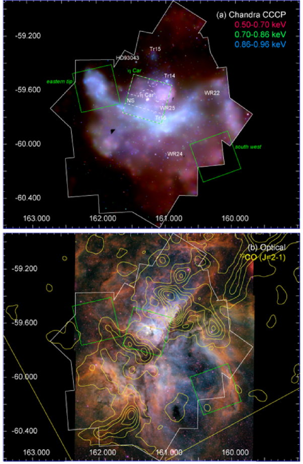
Figure 1: (a) Color-coded Chandra X-ray (red: 0.5–0.7 keV, green: 0.7–0.86 keV, blue: 0.86–0.96 keV) image of the Carina nebula provided from the CCCP (Townsely et al., 2011a). The white labels indicate major massive stellar clusters, massive O main-sequence/Wolf-Rayet stars and the middle-age neutron star (NS) (Hamaguchi et al., 2009). (b) Optical emission line (blue: oxygen, green: hydrogen, red: sulfur) image of the Carina nebula (Nathan Smith, University of Minnesota/NOAO/AURA/NSF, See https://www.noao.edu/image_gallery/html/im0667.html). The blue/red structures tend to be emitted from hotter/cooler ionized gases. The yellow lines show a ¹²CO (J$=$2-1) contour map and the mapping boundary (Yonekura et al., 2005). (a&b) The three green boxes show the FOV of the Suzaku XIS observations used for the diffuse emission — the eastern-tip, $\eta$ Car, and southwest regions from left. The white dash lines in the $\eta$ Car region show subdivided areas (north, south) for analysis in Hamaguchi et al. (2007). The solid white line shows the CCCP survey area. Coordinates are J2000. A 5^′ angular scale corresponds to 3.4 pc at $d$ = 2.3 kpc.

This paper studies diffuse X-ray emission from a southwest region of the Carina nebula using the X-ray data obtained with the Suzaku observatory in 2010. This is the third and final observation of the Carina nebula with Suzaku, whose mission ended in 2015 August. This observing field is distinctively red in the Chandra CCCP X-ray true color image, i.e., very soft X-ray emission. This study aims to understand the cause of this redness with the Suzaku’s good sensitivity and energy resolution in the soft X-ray band.

2 Observation

The X-ray astronomy satellite Suzaku (Mitsuda et al., 2007) observed a southwest region of the Carina nebula on 2010 December 12 (observation ID : 505075010). At the time of this observation, Suzaku operated two types of detectors, the X-ray Imaging Spectrometer (XIS: Koyama et al. (2007)) and the Hard X-ray Detector (HXD: Takahashi et al. (2007)). We use only the XIS, which are sensitive to the soft X-ray emission from the diffuse plasma. Three XIS cameras were available during the observation; two of them (XIS0, 3) have front-illuminated (FI) CCDs and one (XIS1) has a back-illuminated (BI) CCD. The XIS2 camera was lost in 2006 due to a micrometeoroid impact. The Suzaku XISs have lower particle background, higher effective area and better energy resolution for soft extended sources than instruments onboard earlier or ongoing X-ray observatories. They are, therefore, suited best for observing diffuse X-ray emission from the Carina nebula.

We download the final processing data from the HEASARC archive (processing version 3.0.22.43) and analyze the standard cleaned event data using the HEAsoft analysis package version 6.21. We exclude events detected at the flickering pixels that are identified by the instrument team from non X-ray background (NXB) data throughout the Suzaku mission. This procedure completely excludes noise events in the low energy band, which are significant in the later Suzaku observing cycle. We produce background images and spectra with these NXB data using xisnxbgen. The total exposure time is 47.0 ks.

3 Spatial distribution

Figure 1 shows a true color Chandra X-ray image of the Carina nebula provided by the CCCP project (Townsely et al., 2011a) and an optical emission line image with ¹²CO contours. In figure 1 (a), the surface brightness is the highest near the image center, offset from the active star forming clusters, Trumpler 14 and 16 to the south. In this X-ray image, the two blue streaks emanate from this brightest region to the east-northeast and northwest directions. The area between eta Carinae and Trumpler 14 also has high surface X-ray brightness, but the X-ray color is redder than those of the two streaks. The surface brightness is lower and the color is redder toward the southern outskirts.

The first Suzaku study of the diffuse X-ray emission (Hamaguchi et al., 2007) covered the high surface brightness regions. The north and south regions were analyzed separately as their spectra show distinct differences at $\sim$1 keV. The second study (Ezoe et al., 2009) covered the crescent-like plasma structure at the tip of the east-northeast blue streak. The third Suzaku study described in this paper focuses on a red blob near a southwest edge of the CCCP survey field. The rightmost green box in Figure 1 (a) shows the XIS FOV of this observation, a half of which is outside of the CCCP survey field.

Figure 2 shows soft (0.2$-$2 keV) and hard (2$-$5 keV) band images of the Suzaku XIS observation of the southwest region. For each image, the NXB contribution is estimated from night Earth observations with xisnxbgen and subtracted from the raw image. Then, the vignetting effect is corrected with a flat field map at 1.49 keV, which is generated with xissim. The soft band image shows a small flux enhancement around the center, which is seen as a blob in the CCCP image (Figure 1a). The hard band image shows an enhancement in the upper left where the CCCP project detected multiple point sources (Townsely et al., 2011a).

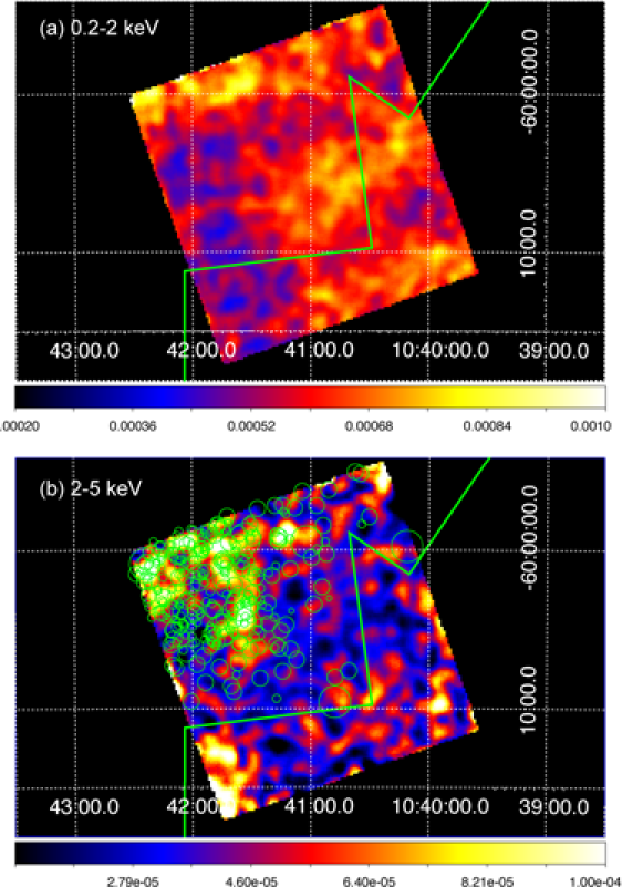
Figure 2: (a) Suzaku XIS1 images of the southwest region of the Carina nebula in the (a) 0.2–2 keV and (b) 2–5 keV bands. These images are smoothed by a 2-dimensional Gaussian function with $\sigma=$5 pixel. The green solid lines indicate the boundary of the CCCP image (the upper left side was imaged.). The green circles in the lower panel show positions of the Chandra point sources (Townsely et al., 2011a). The radius of each circle expresses the 0.5–8 keV flux of the corresponding source in Broos et al. (2011); $r=$10¨for $<$F_X 10^-16, 15¨for 10${}^{-16}\sim$10^-15, 30¨for 10${}^{-15}\sim$10^-14, and 60¨for $>$10^-14 erg s^-1 cm^-2. The coordinates system is J2000.

4 Spectral Analysis

We extract XIS FI (XIS0$+$3) and BI (XIS1) spectra of the whole FOV (figure 3) and generate the corresponding NXB spectra from the night Earth data using xisnxbgen. The source and background spectra of each sensor match well above $\sim$10 keV where the XIS have no sensitivity in X-rays, confirming that the NXB spectra are reproduced correctly. The 0.2–5 keV count rates before and after subtracting the NXB are 0.793$\pm$0.004 and 0.723$\pm$0.004 counts s^-1 for BI and 0.333$\pm$0.002 and 0.305$\pm$0.002 counts s^-1 for one FI where the errors are 1$\sigma$.

The NXB subtracted spectra (figure 4 for BI) show emission lines from highly ionized ions of various elements. such as Ovii, Oviii, Neiv, Nex, Mgxi, and Sxv. Townsely et al. (2011b) reported a marginal emission line at 1.3 keV from the Carina SW region, but the Suzaku spectra show no emission line at this energy.

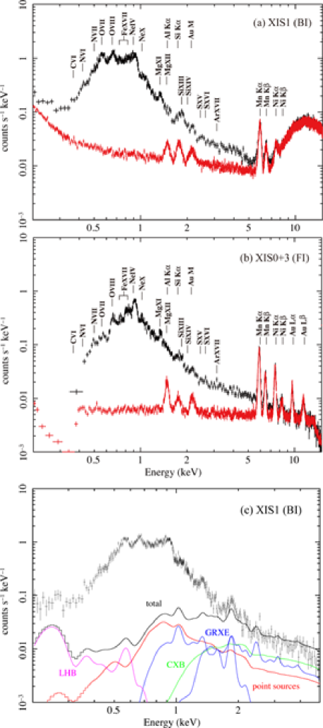
Figure 3: Suzaku BI (a) and FI (b) spectra of the whole XIS FOV (black). The red spectra show show NXB contribution, estimated from the night Earth observations. The labels denote emission lines detected in the source and/or background spectra. (c) Background-subtracted BI spectrum of the whole XIS FOV. The solid lines indicate estimated contamination contributions.

4.1 Contamination from astrophysical backgrounds and point sources

The extracted spectra still include background or foreground sources — local hot bubble (LHB), galactic ridge X-ray emission (GRXE), cosmic X-ray background (CXB), and point sources mostly unresolved with Suzaku. We estimate contributions of LHB, GRXE, and CXB by following the method in Ezoe et al. (2009) and Hamaguchi et al. (2007).

We then estimate contribution of X-ray point sources inside the Suzaku FOV using the CCCP product. Chandra observed this field, labelled as Supperbubble3 (SB3), twice in 2008 May 24 and 31 (ObsID 9498 and 9859) for 31.9 ks and 26.8 ks, respectively. The CCCP catalogue (Broos et al., 2011) lists 400 point sources inside the Suzaku FOV, whose average flux was 2.7$\times 10^{-15}$ erg s^-1 cm^-2 between 0.2–5 keV. A combined Chandra spectrum of these point sources provided by the CCCP team (Private Comm.: Broos, P.) extends up to $\sim$8 keV (figure 4), suggesting a very hot plasma or flat power-law emission. The spectrum also shows line-like structures below $\sim$1 keV, suggesting significant contribution of cool thermal plasma emission from low-mass young stars in the field. We fit the spectrum by a model with a single-temperature plasma emission component (apec) plus a power-law component, both of which suffer interstellar absorption to the Carina nebula. The elemental abundance of the thermal component is fixed at 0.3 solar, the typical abundance of stellar X-ray plasma (e.g., Getman et al. (2005)). We use the corresponding response (rmf) and ancillary response (arf), weighted for the source fluxes.

The best-fit of the apec $+$ power-law model has a residual at $\sim$1 keV, not acceptable with $\chi^{2}$/d.o.f. at 1.75. Adding a narrow Gaussian line significantly improves the fit in an F-test ($\sim$98 %) with $\chi^{2}$/d.o.f. at 1.28. The best-fit centroid energy is consistent with a Ne X Ly_α line (1022 eV). Assuming non-equilibrium plasma emission model (nei) also improves a fit with similar $N_{\rm H}$ and $kT$ and an ionization parameter at $\tau=1.3^{+3.3}_{-1.0}$ s cm^-3. However, the $\chi^{2}$/d.o.f. is 1.41, worse than the model with a Gaussian line. Therefore, we employ the second apec $+$ Gaussian $+$ power-law model to reproduce the point source flux. The best-fit model is shown in table 1. The total X-ray fluxes in the 0.2–2 keV and 2–5 keV bands are 7.1$\times 10^{-13}$ erg s^-1 cm^-2 and 3.7$\times 10^{-13}$ erg s^-1 cm^-2, respectively.

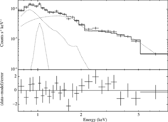
Figure 4: Average Chandra ACIS-I spectrum of the CCCP point sources. The dotted lines show the individual components of the best-fit model.

Table 1: The best-fit result of the average Chandra point source spectrum. The model assumes tbabs (apec + Gaussian + power-law).

Interstellar absorption
$N_{\rm H}$ (1022 cm2)	0.053 ($<$0.252)
Plasma component∗
$kT$ (keV)	0.74$\pm 0.10$
$Z$ (solar)	0.3 (fixed)
Normalization	3.5${}^{+4.6}_{-1.2}\times 10^{-7}$
Gaussian component
$E_{\rm center}$	1.04${}^{+0.03}_{-0.02}$
$\sigma$	0 (fixed)
Normalization (photons s-1 cm-2)	1.5${}^{+0.3}_{-0.1}\times 10^{-8}$
Power law component†
$\Gamma$	1.0$\pm 0.1$
Normalization (keV-1 s-1 cm-2 at 1 keV)	2.1${}^{+0.3}_{-0.2}\times 10^{-7}$
X-ray flux, luminosity§
$F_{\rm X}$ in 0.3–7 keV (erg s-1 cm-2)	2.3$\times 10^{-15}$
$L_{\rm X}$ in 0.3–7 keV (erg s-1)	3.6$\times 10^{29}$
$\chi^{2}$/d.o.f	1.28
d.o.f	19

^∗ The normalization is defined as $10^{-14}/(4\pi D^{2})EM$, where $D$ is the distance to the Carina nebula in cm and $EM$ is the plasma emission measure in cm^-3. The elemental abundances are given relative to the solar photospheric values measured by Anders & Grevesse (1989).
^§ A distance of 2.3 kpc is assumed. The total flux and luminosity of all point sources are $\times$400 of these values.

Figure 3 (c) plots these contamination components on the XIS1 spectrum. The X-ray collecting area changes with the position and spatial distribution of the source on the detector. The collecting area for each emission component is calculated with xissimarfgen and the result is stored in an arf file. For the Chandra point sources, we assume a Chandra ACIS image between 0.5–7 keV taken on 2008 May 24 (ObsID 9498), which has a longer exposure of the two Supperbubble3 observations, as the point source distribution. For the other components, we do not expect strong spatial variation in arcmin scales, and thus we assume uniform surface brightness within 20^′ from the detector center. We reproduce the XIS1 spectra of the contamination components using these arfs.

The total of the contamination spectra matches moderately well with the observed spectrum above 2 keV. This means that the high energy spectrum mostly originates from GRXE and CXB. The small discrepancy can be explained by i) some point sources are active galactic nuclei, whose contribution is also counted in the CXB, ii) Chandra detected point sources only from a half of the XIS FOV, and iii) the CXB fluctuates $\sim$5% (1 $\sigma$) in the sky (Kushino et al., 2002).

Below $\sim$0.4 keV, the observed spectrum is a factor of $\sim$3 higher than the total spectrum of the known source, mostly the LHB. This excess emission should originate from a foreground source as soft X-ray emission below 0.4 keV from sources more distant than the Carina nebula is totally obscured by interstellar absorption. An obvious candidate is the solar wind charge exchange (SWCX) — an interaction of solar winds with material around the Earth (e.g., Snowden et al. (2004); Fujimoto et al. (2009); Ezoe et al. (2010, 2011); Ishikawa et al. (2013)) — which produces multiple emission lines below 1 keV. However, this component correlates with the solar wind intensity and varies on typical timescales of 1$-$10 ksec, but the XIS1 light curve between 0.2–0.6 keV does not show any significant variation. In addition, average proton and ion (C⁶⁺ and O⁷⁺) fluxes of the solar wind, measured with the solar wind monitoring satellites WIND and ACE, are $\sim$5 times smaller around this observation than those during earlier SWCX events observed with Suzaku. These results do not suggest the contamination of significant SWCX emission during this observation. This soft excess may originate from a local enhancement of the LHB emission.

4.2 Spectral fitting

The observed spectrum between 0.4$-$1.5 keV is 2$-$30 times higher than the sum of these contamination components in count rates and therefore should originate mostly from truly diffuse X-ray plasma in the Carina nebula. We simultaneously fit the XIS BI and FI spectra to constrain the spectral parameters. For the truly diffuse component, we assume an absorbed (phabs) two temperature collisional equilibrium plasma (apec) model, which is also used for earlier Suzaku studies of the Carina nebula. For the cosmic background and foreground emission, we add a power-law model to reproduce the hard spectrum above 2 keV and a thermal (apec) model to reproduce the soft spectrum below 0.4 keV. For the instrumental response, we use arf files that assume uniformly extended emission.

Elemental abundances of O, Ne, Mg, Si, S, and Fe, whose emission lines are seen clearly in the spectra (figure 3), are allowed to vary independently, while those of the other elements are fixed at 0.3 solar values. Figure 5 and Table 2 show the best-fit result. We calculate the X-ray fluxes and luminosities in 0.4–5 keV where the diffuse X-ray emission dominates. Also as a reference, we also show the X-ray fluxes between 0.5–7 keV, which is often used for Chandra studies of diffuse X-ray emission from star forming regions.

The hydrogen column density, $N_{\rm H}\sim$1.9$\times 10^{21}$ cm^-2, is similar to those of the other Carina regions (1.2$-$2.4$\times 10^{21}$ cm^-2, Hamaguchi et al. (2007); Ezoe et al. (2009)). The plasma temperatures, $\sim$0.17 and 0.50 keV, are only slightly lower than those of diffuse X-ray plasmas in the other Carina regions studied with Suzaku (0.20–0.25 keV and 0.54–0.60 keV, Hamaguchi et al. (2007); Ezoe et al. (2009)). This result suggests that the plasma are heated in a similar mechanism to those in the other Carina nebula regions.

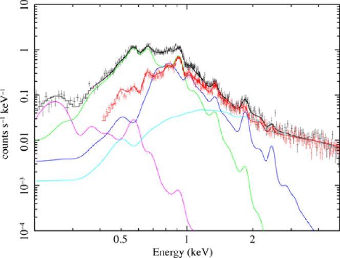
Figure 5: The NXB subtracted spectra of the whole XIS FOV. The black and red solid lines show the best-fit model for the BI and FI spectra. The solid lines in the other colors show the best-fit of the individual components for the XIS1 spectrum.

Table 2: The best-fit two-temperature plasma model for spectra of the whole region and subdivided regions.

Modela	whole region	inner	outer
Two-temperature plasma componentb
$N_{\rm H}$ (1022 cm-2)	0.189$\pm{0.002}$	0.169${}^{+0.026}_{-0.021}$	0.168$\pm{0.032}$
$kT_{1}$ (keV)	0.166$\pm{0.002}$	0.165$\pm{0.008}$	0.174${}^{+0.006}_{-0.008}$
$kT_{2}$ (keV)	0.494${}^{+0.022}_{-0.015}$	0.496${}^{+0.052}_{-0.050}$	0.507${}^{+0.060}_{-0.044}$
O (solar)	0.26$\pm{0.01}$	0.24${}^{+0.05}_{-0.03}$	0.23${}^{+0.03}_{-0.02}$
Ne (solar)	0.55${}^{+0.02}_{-0.03}$	0.49${}^{+0.09}_{-0.07}$	0.48$\pm{0.06}$
Mg (solar)	0.38${}^{+0.03}_{-0.04}$	0.36${}^{+0.11}_{-0.08}$	0.30${}^{+0.08}_{-0.07}$
Si (solar)	0.60${}^{+0.08}_{-0.11}$	0.61${}^{+0.29}_{-0.20}$	0.50${}^{+0.18}_{-0.15}$
S (solar)	1.13$\pm{0.26}$	$1.51^{+1.16}_{-0.73}$	0.80${}^{+0.70}_{-0.58}$
Fe (solar)	0.32${}^{+0.01}_{-0.02}$	0.30${}^{+0.08}_{-0.05}$	0.25${}^{+0.11}_{-0.08}$
log$EM_{1}$ (cm-3 arcmin-2)	55.28$\pm{0.02}$	55.37${}^{+0.11}_{-0.10}$	55.22${}^{+0.12}_{-0.11}$
log$EM_{2}$ (cm-3 arcmin-2)	54.02$\pm{0.02}$	54.03${}^{+0.09}_{-0.08}$	54.01${}^{+0.07}_{-0.08}$
Flux1 in 0.4–5 keV (10-14 erg s-1 cm-2 arcmin-2)	2.5$\pm 0.1$	3.3${}^{+1.0}_{-0.6}$	2.6${}^{+0.8}_{-0.7}$
in 0.5–7 keV (10-14 erg s-1 cm-2 arcmin-2)	2.2$\pm 0.1$	2.9${}^{+0.9}_{-0.5}$	2.3${}^{+0.7}_{-0.6}$
Flux2 in 0.4–5 keV (10-14 erg s-1 cm-2 arcmin-2)	0.80$\pm 0.05$	0.90${}^{+0.10}_{-0.17}$	0.76${}^{+0.14}_{-0.13}$
in 0.5–7 keV (10-14 erg s-1 cm-2 arcmin-2)	0.79$\pm 0.05$	0.88${}^{+0.10}_{-0.16}$	0.75${}^{+0.14}_{-0.13}$
Luminosity1 in 0.4–5 keV (1034 erg s-1)	2.03$\pm$0.08	0.43${}^{+0.17}_{-0.08}$	0.72${}^{+0.23}_{-0.18}$
in 0.5–7 keV (1034 erg s-1)	1.69$\pm$0.07	0.35${}^{+0.10}_{-0.07}$	0.60${}^{+0.19}_{-0.15}$
Luminosity2 in 0.4–5 keV (1034 erg s-1)	0.34$\pm$0.02	0.064${}^{+0.006}_{-0.011}$	0.12$\pm{0.02}$
in 0.5–7 keV (1034 erg s-1)	0.32$\pm$0.02	0.060${}^{+0.006}_{-0.011}$	0.11 $\pm{0.02}$
Power-law componentc
Flux in 0.4–5 keV (10-14 erg s-1 cm-2 arcmin-2)	0.54${}^{+0.02}_{-0.01}$	0.49${}^{+0.04}_{-0.03}$	0.55$\pm{0.03}$
LHB componentd
Flux in 0.4–5 keV (10-14 erg s-1 cm-2 arcmin-2)	0.05$\pm 0.01$	0.05 (fixed)	0.04$\pm{0.02}$
$\chi^{2}$/d.o.f.	1.23	1.09	1.17
d.o.f.	723	255	427

^a Fitting models. Fitting errors at the 90% confidence level are shown. The luminosity is corrected for absorption.
^b phabs * (apec $+$ apec $+$ power-law) $+$ apec (LHB). Abundances of elements that are not shown in this table are fixed at 0.3 solar values. The absolute solar abundance tables are referred to Anders & Grevesse (1989). ^c The photon index is fixed at 1.5. The same absorption for the two-temperature plasma is assumed.
^d The single-temperature plasma model representing LHB. A plasma temperature is fixed at 0.1 keV. No absorption is assumed for this foreground component.

4.3 Multiple absorption models

Townsely et al. (2011b) adopted a multi-temperature non-equilibrium (NEI) plasma model components, each of which suffer individual absorption. With the high photon statistics of the Suzaku XIS spectra, we test these possibilities. We try a two-temperature collisional ionization (CIE) plasma model assuming different absorption for the individual temperature component. The result is shown in figure 6 (a) and table 3. The reduced chi-square value is not significantly better than that of the common absorption model. The absorption column of the hot component is not well constrained while the other parameters are similar to those of the common absorption model.

We also try a two-temperature NEI plasma components suffering different absorptions. We adopt vpshock, following to Townsely et al. (2011b). The result is shown in figure 6 (b) and table 3. The reduced chi-square value is is slightly worse than that of the previous models. The upper limit of $\tau_{\rm u}$ is near the CIE timescale of $\sim 3\times 10^{12}$ s cm^-3, as expected from the acceptable fittings of the CIE models.

These multiple absorption models therefore do not significantly improve the spectral fits. Below we employ the two-temperature CIE plasma model with common absorption for further analysis and discussion.

Table 3: Multiple absorption model fitting results for spectra of the whole region.

Model	CIEa	NEIb
$N_{\rm H1}$ (1022 cm-2)	0.181${}^{+0.005}_{-0.008}$	0.125$\pm{0.017}$
$kT_{1}$ (keV)	0.169$\pm{0.003}$	0.213${}^{+0.007}_{-0.014}$
$N_{\rm H2}$ (1022 cm-2)	0.253${}^{+0.018}_{-0.022}$	0.275${}^{+0.110}_{-0.105}$
$kT_{2}$ (keV)	0.486${}^{+0.082}_{-0.013}$	0.681${}^{+0.065}_{-0.059}$
O (solar)	0.25${}^{+0.02}_{-0.01}$	0.22$\pm{0.01}$
Ne (solar)	0.53${}^{+0.03}_{-0.02}$	0.41$\pm{0.03}$
Mg (solar)	0.37${}^{+0.04}_{-0.03}$	0.26$\pm{+0.03}$
Si (solar)	0.54${}^{+0.07}_{-0.09}$	0.28$\pm{0.06}$
S (solar)	0.95$\pm{0.23}$	0.26${}^{+0.18}_{-0.17}$
Fe (solar)	0.38${}^{+0.02}_{-0.05}$	0.24${}^{+0.04}_{-0.03}$
$\tau_{\rm l}$ (1010 s cm-3)	–	1.0 (fixed)
$\tau_{\rm u}$ (1011 s cm-3)	–	8.0${}^{+3.2}_{-2.8}$
log$EM_{1}$ (cm-3 arcmin-2)	55.25${}^{+0.02}_{-0.01}$	54.87$\pm{0.08}$
log$EM_{2}$ (cm-3 arcmin-2)	54.06$\pm{0.03}$	54.05${}^{+0.09}_{-0.15}$
Flux1 in 0.4–5.0 keV (10-14 erg s-1 cm-2 arcmin-2)	2.6$\pm 0.1$	2.6$\pm{0.5}$
in 0.5–7.0 keV (10-14 erg s-1 cm-2 arcmin-2)	2.3$\pm 0.1$	2.4${}^{+0.5}_{-0.4}$
Flux2 in 0.4–5.0 keV (10-14 erg s-1 cm-2 arcmin-2)	0.77${}^{+0.06}_{-0.05}$	0.74${}^{+0.16}_{-0.22}$
in 0.5–7.0 keV (10-14 erg s-1 cm-2 arcmin-2)	0.76${}^{+0.06}_{-0.05}$	0.74${}^{+0.16}_{-0.22}$
Luminosity1 in 0.4–5.0 keV (1034 erg s-1)	1.94$\pm{0.07}$	1.38${}^{+0.29}_{-0.25}$
in 0.5–7.0 keV (1034 erg s-1)	1.61$\pm{0.06}$	1.10${}^{+0.23}_{-0.19}$
Luminosity2 in 0.4–5.0 keV (1034 erg s-1)	0.40${}^{+0.03}_{-0.02}$	0.41${}^{+0.09}_{-0.10}$
in 0.5–7.0 keV (1034 erg s-1)	0.38${}^{+0.03}_{-0.02}$	0.39${}^{+0.08}_{-0.10}$
Power-law componentc
Flux in 0.4–5.0 keV (10-14 erg s-1 cm-2 arcmin-2)	0.52${}^{+0.02}_{-0.01}$	0.49${}^{+0.01}_{-0.03}$
LHB componentd
Flux in 0.4–5.0 keV (10-14 erg s-1 cm-2 arcmin-2)	0.04$\pm 0.01$	0.04$\pm{0.01}$
$\chi^{2}$/d.o.f.	1.23	1.25
d.o.f.	722	721

^a Two-temperature CIE plasma model with a multiple absorption model: phabs * apec $+$ phabs * apec $+$ phabs * power-law $+$ raymond. ^b Two-temperature NEI plasma model with a multiple absorption model: phabs * vpshock $+$ phabs * vpshock $+$ phabs * power-law $+$ raymond. $\tau_{\rm l}$ and $\tau_{\rm u}$ are lower and upper limits on ionization timescale, respectively. ^c The photon index is fixed at 1.5. In the multi absorption model, the larger absorption for the two-temperature plasma, i.e., $N_{\rm H2}$, is assumed for this background component. ^d The single-temperature plasma model representing LHB. A plasma temperature is fixed at 0.1 keV. No absorption is assumed for this foreground component.

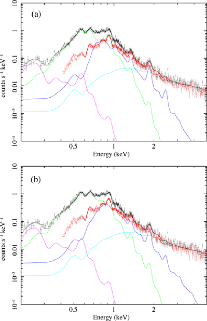
Figure 6: The same as figure 5 but for two-temperature (a) CIE and (b) NEI plasma model with different absorptions. See table 3 for the obtained parameters.

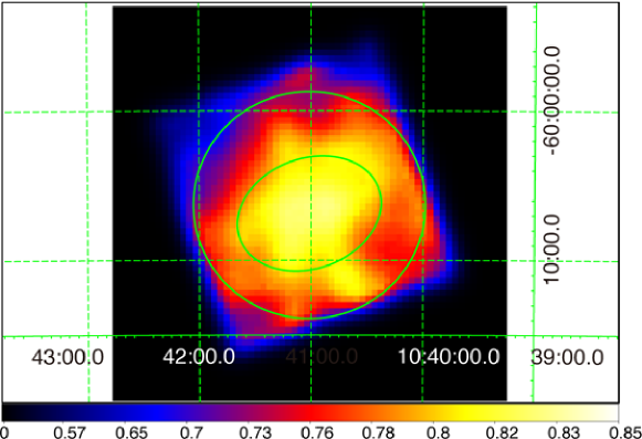
Figure 7: Hardness ratio map by calculating $(S-H)/(S+H)$ where $H$ and $S$ are 0.8–2.0 keV and 0.4–0.8 keV XIS1 images. Before division, the NXB is subtracted from each image binned by 3 pixels for limited photon statistics. For clarity, the hardness ratio map is smoothed by a 2-dimensional Gaussian function with $\sigma=5$ pixels. Solid lines indicate two subdivided regions.

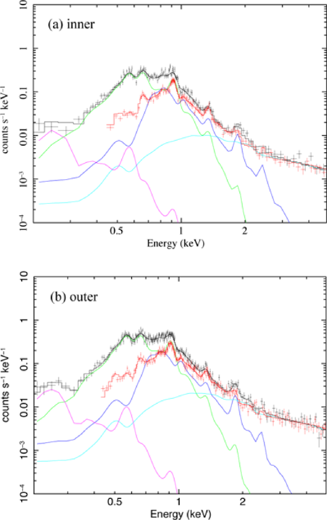
Figure 8: The same as figure 5 but for (a) the inner and outer regions. See table 2 for the obtained parameters.

4.4 Subdivided regions

We then investigate spatial variation of the diffuse spectrum. We create a map of of the hardness ratio defined from images that correct the spatial effective area variation due to the mirror vignetting and OBF contamination The map in figure 7 shows significant softness toward the FOV center where the red blob is. In fact, the blob is clearly seen in the 0.4–0.8 keV image but not in the 0.8–2 keV image. This result suggests that the blob originates from the spatial structure of the cool component.

We therefore define two regions in the XIS FOV based on this hardness ratio map; the inner region with the softest color and the outer region that is the outskirt. We extract their spectra and fit them using the two-temperature CIE plasma model with common absorption. The sizes of the inner and outer regions are 57 and 127 arcmin² for each, which correspond to 25 and 57 pc² at a distance of 2.3 kpc, respectively.

The applied model reproduces the two spectra well (figure 8 and table 2). Their best-fit parameters are very similar to those of the whole region within 90 % statistical uncertainties. We fix the flux of the LHB component for the inner region at the best fit value of the whole region because it became unreasonably low (0.6$\times 10^{-14}$ erg s^-1 cm^-2 arcmin^-2) if it is a free parameter probably due to the limited statistics below 0.4 keV. Since the spatial variation of the LHB component on arcmin scales is not likely, we fix this parameter. The obtained reduced chi-square is acceptable.

The total flux of the point sources detected with Chandra in the inner and outer regions is $\sim$5$\times 10^{-14}$ and $\sim$3$\times 10^{-13}$ erg s^-1 cm² at 0.4–5 keV, whose contribution is $\sim$2 % and $\sim$6 % for the diffuse X-ray emission in the inner and outer regions, respectively. Therefore, similar to the whole region, the diffuse X-ray emission is dominant.

The inner region has a $\sim$30% larger flux of the cool component than the outer region, while there was $\sim$20 % difference in the flux of the hot component. This result may confirms that the cool component produces the blob-like structure.

To check possible variation of absorption column density, we apply the best fit model of the inner region to the outer region spectra while a scaling factor and an additional absorption for the two temperature plasma component are free. The fitting is acceptable with $\chi^{2}$/d.o.f. of 1.20, the scaling factor of 1.01$\pm 0.02$ and the additional $N_{\rm H}$ of $(0.037\pm 0.004)\times 10^{22}$ cm^-2. This correspond to optical extinction $A_{V}$ of $\sim$0.2 (Güver et al., 2009), which is small and not suggested in the past CO and optical observations. Therefore, if there is a variation of the absorption column density, the variation is small. We thus simply employ the commonly absorbed two-temperature plasma model for further discussion below.

5 Discussion

We here compare this result with the previous Suzaku studies. The three Suzaku observations were performed at different periods — the $\eta$ Car region was observed in 2005 August, the eastern-tip region 2006 June, and the Carina SW region 2010 December. An important caveat is that their soft band spectra cannot be directly compared as the XIS’s soft band sensitivity significantly declined between these observations due to contamination on the XIS blocking filter. This sensitivity degradation is considered in arf for spectral fitting (Ishisaki et al., 2007), so we compare the results of their spectral fits, while we cannot directly compare their spectra in count rates due to this difference in sensitivity.

5.1 Spatial Distribution of the Diffuse Plasma

In all studies, the diffuse spectra were reproduced by models with the same components: two temperature thermal plasma emission suffering weak absorption. The only difference in the fitting conditions is that the diffuse spectra around $\eta$ Carina were fitted with a free parameter for the carbon elemental abundance (Hamaguchi et al., 2007). Without any clear carbon emission lines between 0.3$-$0.4 keV, the fit deduced small carbon abundance. A carbon does not provide enough free electrons to the plasma. The hydrogen (and helium) elemental abundance are increased to supply electrons for Bremsstrahlung continuum emission. This resulted in moderately low elemental abundance values to the other heavy elements. However, X-ray emission from the Carina nebula suffers strong cut-off below 0.4 keV, and the spectra below 0.4 keV should be strongly contaminated by foreground emission and/or affected by structures in the instrumental response. Fortunately, this conditional difference does not significantly affect measurements of the key spectral parameters ($N_{\rm H}$, $kT$, $EM$) nor abundance ratios between heavily elements. We thus use the best-fit parameters in table 1 individual models of Hamaguchi et al. (2007) for the $\eta$ Car north and south regions, and table 3 model 1 of Ezoe et al. (2009) for the eastern tip region for comparison.

Figure 9 plots $N_{\rm H}$, $kT$, $EM$ and surface brightness of the hot and cool plasma components. The $N_{\rm H}$ values are similar between the regions. This means that diffuse emission from these regions does not suffer significant local absorption. Even if we adopt the multiple absorption CIE or NEI plasma models, the larger $N_{\rm H}$ value is still small ($\sim$0.3$\times 10^{22}$ cm^-2). This is not surprising for the Carina SW and the eastern tip regions with little molecular gas in their lines of sight (Yonekura et al., 2005). However, both the north and south $\eta$ Car regions have moderate amount of molecular gas columns. This result suggests that i) the molecular gases are not thick enough for the X-ray emission, ii) the molecular gases are much smaller than the spatial resolution of the radio telescope (2.7^′) so that molecular gas does not obscure most X-ray emission, or iii) the molecular gases are behind the X-ray plasma. In either case, absorption does not cause the redness of the Carina SW region.

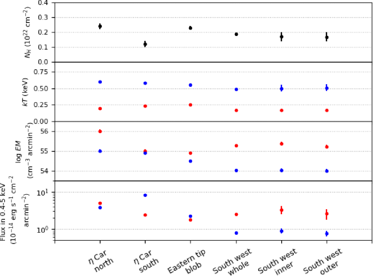
Figure 9: Comparison of the two-temperature plasma model fits ($\eta$Car north/south: table 1 individual models in Hamaguchi et al. (2007), the eastern tip blob region: table 3 model 1 of Ezoe et al. (2009), South west: this work). Blue and red colors represent the hot and cool components.

Both cool and hot plasmas have similar temperatures between the regions; only the Carina SW region has a slightly lower temperature by 0.05$-$0.1 keV in each component than the other regions. The surface brightness of the cool plasma emission lies within a factor of $\sim$2$-$3 between the regions, while that of the hot plasma emission varies by an order of magnitude. The Carina SW region has the lowest surface flux of the hot plasma component, and the lowest relative flux over the cool plasma emission. This is the reason why the Carina SW region is colored in red.

These results suggest that there are physically two distinctive plasma components in the Carina nebula. The plasma temperatures of the Carina SW region are slightly cooler, possibly due to weaker heating and/or stronger cooling near a nebula edge.

5.2 Plasma Elemental Abundances

The spectral fits constrain elemental abundances of O, Ne, Mg, Si, S and Fe from their K or L-shell emission lines seen between 0.4$-$3 keV. The Si and S abundance measurements rely mostly on their K-shell emission lines at $\sim$2 and 2.6 keV, but background emission is comparable to the diffuse emission in this energy range, and some contamination sources such as GRXE and low mass young stars emit those lines as well. We therefore calculate abundance ratios of O, Ne and Mg relative to Fe and compare them with those expected from SNe and stellar wind bubbles.

Figures 10 and 11 plot abundance ratios of all Carina regions. Because the fitting errors of the elemental abundances of the inner and outer regions are relatively large and their values are consistent with those of the whole regions within errors, we plot only the whole region for the Carina SW. Figure 10 also displays abundance ratios of Type Ia and core-collapsed SN remnants derived from theoretical models (e.g., Hughes et al. (1995); Hendrick et al. (2003); Williams & Chu (2005)). The measured abundance ratios of the Carina diffuse nebula fall within 7.3$-$14.8 for O/Fe, 1.2$-$4.5 for Ne/Fe, and 0.5$-$1.1 for Mg/Fe. These values are consistent with those of core collapsed SNe models but significantly higher than the Type Ia SNe model, which are rich in iron.

On the other hand, figure 11 also displays the abundance ratio of wind driven X-ray emission from OB stars; $\delta$Ori (Raassen et al., 2013) and $\tau$Sco (Mew et al., 2003). A caveat is that the $\tau$Sco measurements are apparently worse than the $\delta$Ori measurements, but this is because the Fe abundance was measured independently for $\tau$Sco (0.9$\pm$0.5 solar photospheric value, see table 2 in Mew et al. (2003)). All ratios are similar to those of OB stars.

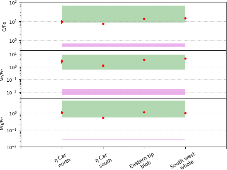
Figure 10: Comparison of the elemental abundance ratios. The filled green box indicates a range of the element abundance ratio based on nucleosynthesis models for Type II SNe with 15–20 $M_{\odot}$ progenitor masses (Nomoto et al., 1997), while the filled magenta box is that for two Type Ia SNe models (W7$=$fast deflagration model and WDD1$=$slow deflagration, delayed detonation model) (Iwamoto et al., 1999).

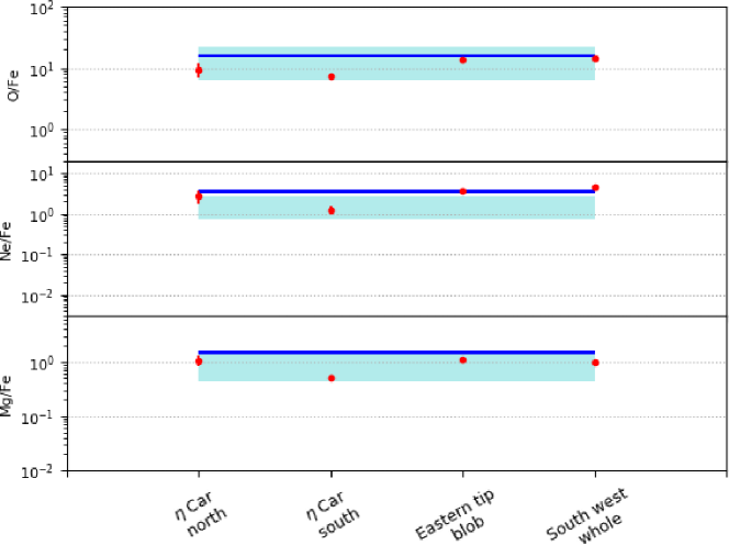
Figure 11: The same as figure 9 but with the ranges of $\delta$Ori (O9.5II, Raassen et al. (2013)) and $\tau$Sco (B0.2V, Mew et al. (2003)). The filled blue and cyan boxes indicate 1$\sigma$ confidence regions for $\delta$Ori and $\tau$Sco, respectively.

5.3 Physical properties of the diffuse plasma

We estimate physical properties of the diffuse plasma in the Carina SW region using the same method as Ezoe et al. (2009). Here we need to assume a shape of the diffuse plasma to estimate its volume. Even though the size of the diffuse plasma in the line of sight direction is unclear, we here simply assume 10 pc from the size of the nebula. A side length of the XIS FOV of 17.8 arcmin corresponds to 11.9 pc at the distance of 2.3 kpc. For each plasma component, we deduce the electron density from the emission measure and the assumed plasma volume and the pressure from the plasma temperature and the electron density. We then calculate the total plasma energy, its cooling time, and the mass using these physical values as follows.

$$L_{\rm X} = \Lambda(T)EM=\Lambda(T)n_{\rm e}^{2}V\eta,$$ (1)

$$U = 3~{}n_{\rm e}kTV,$$ (2)

$$p = 2~{}n_{\rm e}kT,$$ (3)

$$t_{\rm cool} = U/L_{\rm X},$$ (4)

$$M_{\rm plasma} = \mu_{\rm X}~{}m_{\rm p}n_{\rm e}V,$$ (5)

where $\Lambda$, $EM$, $\eta$, and $\mu_{\rm X}$ denote the cooling function, the volume emissivity, a scale factor of the volume of the plasma, and the mean molecular weight per electron. We assumed $\Lambda=$15$\times 10^{-23}$ and 5$\times 10^{-23}$ erg s^-1 cm³ s^-1 for the low and high temperature plasma components and $\mu_{\rm X}=$0.62 as used in Townsely et al. (2003) and Ezoe et al. (2009).

Table 4 shows the result. The estimated plasma density and the pressure of the high and low temperature components are about $\times$5-10 and $\times$10-25 times lower than those in the blob of the easter tip region (table 6 in Ezoe et al. (2009)). Although these pressures can be lower than those of the plasma near $\eta$Car and the eastern-tip region, they are still comparable to those of molecular clouds. Since no strong CO emission is observed in this region (Yonekura et al., 2005) (see figure 1), the plasma pressures of the two temperature components are still larger than ambient materials and can continue to expand.

Another important point is that the cooling times are longer than a typical life time of OB stars (0.1-1 Myr) and also a propagation time of the plasma at sound velocity from the center of this nebula (i.e., near $\eta$Car) to this area (on the order of 0.1 Myr). Therefore, this may support the scenario that plasma generated around the center of the Carina nebula via stellar winds of OB stars or SNe propagates toward the surrounding region but the plasma pressure slightly drops due to expansion.

Table 4: Physical properties of the diffuse plasma in the whole region^a.

Parameter	Scale Factor	$T_{1}$	$T_{2}$
Observed X-ray Properties
$kT$ (keV)	$-$	0.2	0.5
$L_{\rm X}$ (ergs s-1)	$-$	2$\times 10^{34}$	3$\times 10^{33}$
$V$ (cm3)	$\eta$	4$\times 10^{58}$	4$\times 10^{58}$
Estimated X-ray Plasma Properties
$n_{\rm e}$ (cm-3)	$\eta^{-1/2}$	0.06	0.04
$P/k$ (K cm-3)	$\eta^{-1/2}$	2$\times 10^{5}$	2$\times 10^{5}$
$U$ (ergs)	$\eta^{1/2}$	2$\times 10^{48}$	2$\times 10^{48}$
$t_{\rm cool}$ (yr)	$\eta^{1/2}$	3$\times 10^{6}$	2$\times 10^{7}$
$M_{\rm plasma}$ ($M_{\odot}$)	$\eta^{1/2}$	1.2	0.5

^a $\eta$ is a scale factor for the volume of the plasma. $T_{1}$ and $T_{2}$ indicate the two temperature plasma component in table 2.

5.4 Implications on the SNe and stellar wind bubble scenario

These arguments suggest that there are two diffuse plasma components in the Carina nebula: hot (kT $\sim$0.5-0.6 keV) plasma concentrated in the center of the nebula and the cool (kT $\sim$0.2-0.3 keV) plasma extended throughout the nebula. Their plasma temperatures fit with both the core-collapsed SNe and stellar wind bubble scenario. Relatively young ($\lesssim 10^{4}$ yr) core-collapsed SNe have $kT$ of 0.1–1 keV plasma in ionization equilibrium (e.g., Williams & Chu (2005)). Stellar wind bubbles from OB stars can also produce a shock temperature of $\sim$1 keV with 1000 km s^-1 velocity winds (Ezoe et al., 2009).

Townsely et al. (2011c) estimated the total energy of the diffuse plasma in the Carina nebula at $\sim 10^{50}$ ergs. The Carina nebula currently possesses $\sim$66 massive stars, and it is likely that the nebula would have produced more massive stars in the past that exploded as SNe. Indeed, Hamaguchi et al. (2009) discovered a middle-aged neutron star in the Carina nebula, whose progenitor may have erupted as a Type II SN in the nebula.

On the other hand, a single massive star can supply $\sim 3\times 10^{48}$ ergs throughout its lifetime to the interstellar space through wind kinematic energy (e.g., Ezoe et al. (2009)). Even if we assume that this energy is converted to the plasma energy with a certain efficiency (e.g., 0.1 %), the total energy is only $\sim 3\times 10^{45}$ ergs. Therefore, we need $\sim 3\times 10^{4}$ OB stars, which is far larger than the number of the known OB stars in the Carina nebula ($\sim$70). Therefore, the stellar winds only may not explain all thermal energy of the diffuse plasma.

From these points of view, we suggest that the origin of the diffuse plasma in the Carina nebula maybe a combination of Type II SNe and stellar winds or Type II SNe only. Considering the different spatial distribution over the Carina nebula, the two temperature components may have different events/origins.

6 Summary

We investigate diffuse X-ray emission near a south-west edge of the Carina nebula using the Suzaku observatory. We carefully estimate contribution of plausible emission components in the field and conclude that most emission originates from truly diffuse plasma.

The diffuse X-ray spectrum is reproduced by an absorbed two-temperature CIE plasma emission model. Two-temperature CIE and NEI plasma models with multiple absorption columns can also reproduce the data but $\chi^{2}$/d.o.f. values are similar. Therefore, the simple two-temperature CIE plasma emission with single absorption is adopted. The obtained spectral parameters in the absorbed two-temperature CIE plasma emission model are compared to those of the other regions in the Carina nebula. The surface brightness of the hot component is relatively lower than those of the other regions of the Carina nebula and thus the cool plasma is evident. Therefore, the two temperature plasma components may have different origins.

The plasma temperatures and elemental abundances are consistent with the origin of Type II SNe or stellar wind bubbles, while the total energy of the diffuse plasma in the Carina nebula may not be explained by stellar winds from existing OB stars only. The plasmas thus may originate from both the ancient Type II SNe and OB stellar winds or Type II SNe only.

Future high resolution spectroscopy with X-ray microcalorimeters will provide more detailed information of plasma properties such as plasma motions and ionization states which should help understand the origin of diffuse X-ray emission from the Carina nebula.

We thank Leisa Townsley and Patrick Broos for providing us with the CCCP images and the summed spectrum of the point sources. We also would like to acknowledge the Suzaku XIS team for beautiful calibration.

References

- Albacete Colombo et al. (2018) Albacete Colombo, J.F., et al., astro-ph 1806.0123
- Anders & Grevesse (1989) Anders, E., & Grevesse, N. 1989, Geochimica et Cosmochimica Acta, 53, 197
- Broos et al. (2011) Brooks, P.S., Townsley, L.K., Feigelson, E.D., Getman, K.V., Garmire, G.P., Preibisch, T., Smith, N., Babler, B.L., Hodgkin, & S., Indebetouw, R. 2011, ApJS, 194, 2
- Castor et al. (1975) Castor, J., McCray, R., Weaver, R. 1975, ApJ, 200, L107
- Cunha & Lambert (1994) Cunha, K., & Lambert, D. L. 1994, ApJ, 426, 170
- Daflon, Cunha & Butler (2004) Daflon, S., CunHa, A, & Butler, K. 2004, ApJ, 604, 326
- Dicky & Lockman (1990) Dickey, J. M., & Lockman, F. J. 1990, ARA&A, 28, 215
- Ezoe et al. (2006a) Ezoe, Y., Kokubun, M., Makishima, K., Sekimoto, Y., Matsuzaki, K. 2006a, ApJ, 638, 860
- Ezoe et al. (2006b) Ezoe, Y., Kokubun, M., Makishima, K., Sekimoto, Y., Matsuzaki, K. 2006b, ApJ, 649, L123
- Ezoe et al. (2009) Ezoe, Y., Hamaguchi, K., Güdel, Chu, Y.-H, Petre, R., Corcoran, M.F. 2009, PASJ, 61, S123
- Ezoe et al. (2010) Ezoe, Y., Ebisawa, K., Yamasaki, N. Y., Mitsuda, K., Yoshitake, H.,Terada, N., Miyoshi, M., Fujimoto, R. 2010, PASJ, 62, 981
- Ezoe et al. (2011) Ezoe, Y., Miyoshi, Y., Yoshitake, H., Mitsuda, K., Terada, N., Oishi, S., Ohashi, T. 2011, PASJ, 63, S691
- Feigelson et al. (1997) Feigelson, A., Puls, J., Pauldrach, A.W.A. 1997, ApJ, 322, 878
- Fujimoto et al. (2009) Fujimoto, R., et al. 2007, PASJ, 59, S133
- Getman et al. (2005) Getman, K. V., et al. 2005, ApJS, 160, 319
- Güdel et al. (2008) Güdel, M., Briggs, K. R., Montmerle, T., Audard, M., Rebull, L., Skinner, S. L. 2008, Science, 319, 309
- Güver et al. (2009) Güver, T., Özel, F. 2009, MNRAS, 400, 2050
- Hamaguchi et al. (2007) Hamaguchi, K., et al. 2007, PASJ, 59, S151
- Hamaguchi et al. (2009) Hamaguchi, K., et al. 2009, ApJL, 695, L4
- Hendrick et al. (2003) Hendrick, S. P., Borkowski, K. J., Reynolds, S. P. 2003, ApJ, 593, 370
- Hyodo et al. (2008) Hyodo, Y., Tsujimoto, M., Hamaguchi, K., Koyama, K., Kitamoto, S., Maeda, Y., Tsuboi, Y., Ezoe, Y. 2008, PASJ, 60, 85
- Hughes et al. (1995) Hughes, J.P., Hayashi, I., Helfand, D., Hwang, U., Itoh, M., Kirshner, R., Koyama, K., Markert, T., Tsunemi, H., Woo, J., ApJL, 444, 81
- Ishikawa et al. (2013) Ishikawa, K., Ezoe, Y., Miyoshi, Y., Terada, N., Mitsuda, K., & Ohashi, T. 2013, PASJ, 65, 63
- Ishisaki et al. (2007) Ishisaki, Y., et al. 2007, PASJ, 59, S113
- Iwamoto et al. (1999) Iwamoto, K., Brachwitz, F., Nomoto, K., Kishimoto, N., Umeda, H., Hix, W. R., & Thielemann, F. 1999, ApJS, 125, 439
- Koyama et al. (2007) Koyama, K., et al. 2007, PASJ, 59, S23
- Kushino et al. (2002) Kushino, A., et al. 2002, PASJ, 54, 327
- Mew et al. (2003) Mewe R., Raassen, A.J.J., Cassinelli, J.P., van der Hucht, K.A., Miller, N.A., Güdel, M. 2003, A&A 398, 203
- Mitsuda et al. (2007) Mitsuda, K., et al. 2007, PASJ, 59, S1
- Nomoto et al. (1997) Nomoto, K., Hashimoto, M., Tsujimoto, T., Thielemann, F.-K., Kishimoto, N., Kubo, Y., & Nakasato, N. 1997, Nuclear Physics A, 616, 79c
- Raassen et al. (2013) Raassen, A.J.J., & Pollock, A.M.T. 2013, A&A, 550, A55
- Seward et al. (1979) Seward, F. D., Forman, W. R., Giacconi, R., Griffith, R. E., Harnden, F. R., Jr., Jones, C., & Pye, J. P. 1979, ApJ, 234, L55
- Smith & Brooks (2008) Smith, N., & Brooks, K. J. 2008, in Handbook of Star Forming Regions, Vol. II, ed. B. Reipurth (San Francisco, CA: ASP), 138
- Snowden et al. (2004) Snowden, S. L., Collier, M. R., & Kuntz, K. D. 2004, ApJ, 610, 1182
- Takahashi et al. (2007) Takahashi, T., et al. 2007, PASJ, 59, S35
- Townsely et al. (2003) Townsley, L.K., Feigelson, E.D., Montmerle, T., Broos, P.S., Chu, Y.-H., Garmire, G.P. 2003, ApJ 593, 87
- Townsely et al. (2011a) Townsley, L.K., Broos, P.S., Chu, Y.-H., et al. 2011a, ApJS 194, 16
- Townsely et al. (2011b) Townsley, L.K., Broos, P.S., Chu, Y.-H., et al. 2011b, ApJS 194, 15
- Townsely et al. (2011c) Townsley, L.K., Broos, P.S., Chu, Y.-H., et al. 2011c, ApJS 194, 1
- Tsujimoto et al. (1995) Tsujimoto, T., Nomoto, K., Yoshii, Y., Hashimoto. M., Yanagida. S., & Thielemann, F.-K. 1995, MNRAS, 277, 945
- Weaver et al. (1977) Weaver, R., McCray, R., Castor, J., Shapiro, P., Moore, R. 1977, ApJ 218, 377
- Williams & Chu (2005) Williams, R.M., Chu, Y-H, ApJ, 635, 1077
- Wolk et al. (2002) Wolk, S. J., Bourke, T. L., Smith, R. K., Spitzbart, B., Alves, J. 2002, ApJ, 850, L161
- Yonekura et al. (2005) Yonekura, Y., et al. 2005, ApJ, 634, 476