A least-squares Galerkin approach to gradient and Hessian recovery for nondivergence-form elliptic equations

Abstract.

We propose a least-squares method involving the recovery of the gradient and possibly the Hessian for elliptic equation in nondivergence form. As our approach is based on the Lax–Milgram theorem with the curl-free constraint built into the target (or cost) functional, the discrete spaces require no inf-sup stabilization. We show that standard conforming finite elements can be used yielding a priori and a posteriori convergence results. We illustrate our findings with numerical experiments with uniform or adaptive mesh refinement.

1. Introduction

Elliptic equations in nondivergence form play an important role in many domains of pure and applied mathematics ranging from nonlinear PDEs (Caffarelli and Cabré, 1995; Armstrong and Smart, 2010) to Probability Theory (Evans, 1985; Fabes and Stroock, 1983), continuum Game Theory, homogenization (Capdeboscq et al., 2020) and wave propagation (Arjmand and Kreiss, 2017). The numerical approximation of such equations (references to be given below) plays thus an important role. Here we propose a least-squares based gradient- or Hessian-recovery Galerkin finite element method for the numerical approximating of a function $u:\varOmega\to\mathbb{R}$, $\varOmega$ convex, solving the following linear elliptic Dirichlet boundary value problem in nondivergence form

(1.1) $$\mathcal{{L}}u:=\boldsymbol{{A}}\!:\!\operatorname{D}\!^{2}u+\boldsymbol{b}\cdot\nabla u-cu=f\text{ and }\left.u\right|_{\partial\varOmega}=r$$

where $f\in\operatorname{L}_{2}(\varOmega)$, $r\in\operatorname{H}^{3/2}(\partial\varOmega)$, all coefficients are measurable, $\boldsymbol{{A}}$ is a uniformly elliptic tensor-valued,

(1.2) $$\lambda_{\flat}\boldsymbol{\mathrm{I}}{}\leqslant\boldsymbol{{A}}\leqslant\lambda_{\sharp}\boldsymbol{\mathrm{I}}{},\text{${\ }\text{almost everywhere }$ in }\varOmega,\text{ for some }\lambda_{\sharp}\geqslant\lambda_{\flat}>0,$$

$c$ is non-negative on $\varOmega$ and $\boldsymbol{{A}}$, $\boldsymbol{b}$, $c$ satisfy either of the Cordes condition (2.8) or (2.9) (to be discussed in § 2.2). Roughly speaking, the Cordes condition allows us to reformulate the operator $\mathcal{{L}}$ so that it is close enough to an invertible operator in divergence form thereby ensuring the elliptic problem with discontinuous coefficients is well-posed (see §2.2 for more details).

A main difficulty in the study of elliptic PDEs in nondivergence form is the lack of a natural variational structure which precludes a straightforward use of weak solutions in $\operatorname{H}^{1}(\varOmega)$, say, and their numerical approximation using the bilinear form given by the exact problem. One is thus forced to find some suitable approximation of the Hessian more or less directly. The appropriate concept of generalized solution for nondivergence form equations is that of viscosity solution, which relies on the maximum principle. In this respect, finite difference methods have the advantage over Galerkin methods, in that they replicate more easily the maximum principle, which is very useful when aiming at the approximation of viscosity solutions. On the other hand finite difference methods, besides lacking the geometric flexibility and the higher order approximation power of Galerkin methods, must be modified to take into account coefficients that are more singular than Lipschitz (Froese and Oberman, 2009). Dealing with the boundary is also not that straightforward as with Galerkin methods Which we deal with in this article.

Galerkin methods for general elliptic PDEs in nondivergence form were studied by Böhmer (2010), but $\operatorname{C}^{1}(\varOmega)$ finite elements are required for their practical implementations (Davydov and Saeed, 2013). A recovered Hessian finite element method for approximating the solution of nondivergence form elliptic equation was introduced by Lakkis and Pryer (2011); this method was later generalized and fully analyzed by Neilan (2017). Discontinuous Galerkin approaches have been proposed by Smears and Süli (2013), Feng et al. (2017) and Feng et al. (2018). Further Galerkin approaches for nondivergence form equation do exist such as the two-scale Galerkin method which is based on an integro-differential scheme by Nochetto and Zhang (2018) and the somewhat related method of Feng and Jensen (2017), which draws on the semi-Lagrangian methods and the celebrated convergence theorem of Barles and Souganidis (1991), the primal-dual weak Galerkin method Wang and Wang (2018) and the variational formulation of elliptic problems in nondivergence form of Gallistl (2017).

In this paper, we propose a least-squares approach combined with a gradient and Hessian recovery. Our approach is related to the method of Smears and Süli (2013) in that the test function is the elliptic operator (or an approximation thereof) applied to the “variable function”, but, unlike them, we use conforming finite elements. Our work is also connected to that of Gallistl (2017) with the key departure that our least-squares approach allows a cost-functional enforcement of the curl-free requirement rather than imposing this on the function space and having to enforce it discretely via inf-sup stable discretizations. Indeed, a feature of the method we will propose is that it is coercive and based on the idea of gradient- or Hessian-recovery combined with Lax–Milgram theorem, which as noted by Bramble et al. (1997) it is one of the two main approaches of least squares Galerkin methods (the other is a weighted-residual approach based on the Agmon–Douglis–Nirenberg theory). An obviously non-exhaustive list of references to the least-squares based Galerkin methods for linear and nonlinear we came across is further complemented by Aziz et al. (1985) (based on the ADN theory) Bochev and Gunzburger (2006) (which gives a thorough survey at writing time) Dean and Glowinski (2006) (which uses least-squares to solve the Monge–Ampère equation, related to nondivergence PDEs) and its further refinement Caboussat et al. (2013). We deem it worth noting that an early attempt at least-squares FEMs for elliptic equation in nondivergence form by Bramble and Schatz (1970) is quite inspiring, despite the difficulties in practical implementations of methods there proposed (they require the same $\operatorname{H}^{2}$-conformity as Böhmer (2010)).

The rest of this article is structured as follows: in § 2 we introduce the main background material, the cost (or energy) functional $E_{\theta}$ (where $\theta$ is a parameter) to be minimized and the associated bilinear forms; we give some technical remarks. In § 3 we show that the bilinear forms associated with $E_{\theta}$ satisfy the Lax–Milgram theorem’s assumptions thereby guaranteeing the least-squares problem and the equivalent exact PDE are well-posed. In § 4 we introduce the Galerkin discretization, which, thanks to § 3, enjoys quasi-optimality and convergence properties on general finite element spaces without the need to enforce inf-sup; we also derive via a residual–error a posteriori estimate, indicators and an adaptive algorithm. Finally in § 5 we illustrate the theoretical findings with numerical experiments in both uniform and adaptive mesh refinement frameworks, before giving some conclusions and outlook in § 6.

2. Least-squares approach to elliptic problems in nondivergence form

We now provide the main technical ideas for our approach. After some preliminaries, function spaces in § 2.1, we discuss the Cordes conditions in § 2.2 and the nonhomogenous Dirichlet problem in 2.3. We introduce in 2.4 the least-squares formulation with cost (or energy) functional $E_{\theta}$ of problem (1.1) with $r=0$ and show the equivalence between solving this and the Euler–Lagrange equations in § 2.6 and briefly discussing a Hessian-less variant of our method in Remark 2.7. We close this section by introducing further the bilinear forms in § 2.8 and recalling a useful Maxwell-type estimate of Costabel and Dauge (1999) in Lemma 2.9.

2.1. Basic notation and function spaces

For two vectors $\boldsymbol{x}=\left({x_{1},\dotsc,x_{m}}\right),\boldsymbol{y}=\left({y_{1},\dotsc,y_{m}}\right)$ (displayed as columns with row transposes) in $\mathbb{R}^{m}$ we write $\boldsymbol{x}\cdot\boldsymbol{y}:=\boldsymbol{x}{}^{\intercal}\boldsymbol{y}:=\sum_{i=1}^{m}{x}_{i}y_{i}$. For a matrix, $\boldsymbol{{M}}\in\mathbb{R}^{m\times m}$, $\operatorname{tra}\boldsymbol{{M}}$ denotes the trace of the matrix $\boldsymbol{{M}}$, defined as the sum of its eigenvalues (or, equivalently, its diagonal entries) and $\det\boldsymbol{{M}}$ denotes the determinant of $\boldsymbol{{M}}$ defined as the product of its eigenvalues. For two matrices $\boldsymbol{{M}},\boldsymbol{{N}}\in\mathbb{R}^{m\times l}$, their Frobenius inner product is defined by $\boldsymbol{{M}}\!:\!\boldsymbol{{N}}:=\operatorname{tra}\left({\boldsymbol{{M}}{}^{\intercal}\boldsymbol{{N}}}\right)$ and by $\left|\boldsymbol{{M}}\right|$ we mean the Frobenius norm of the matrix $\boldsymbol{{M}}$, defined as $\left|\boldsymbol{{M}}\right|:={\left({\boldsymbol{{M}}\!:\!\boldsymbol{{M}}}\right)}^{\nicefrac{{1}}{{2}}}$, which coincides with the Euclidean norm of $\boldsymbol{{M}}$’s spectrum.

Throughout the paper, including the above we denote, for a function (or distribution) $\boldsymbol{\phi}:\varOmega\to\mathbb{R}^{m}$, $m\in\mathbb{N}$, by $\operatorname{D}\!\boldsymbol{\phi}$ its first derivative, $\nabla\boldsymbol{\phi}:=\left({\operatorname{D}\!\boldsymbol{\phi}}\right)^{\intercal}$ its gradient and, when $m=1$ (with a slight abuse of notation) by $\operatorname{D}\!^{2}\boldsymbol{\phi}$ its Hessian (matrix or tensor). We shall also denote the divergence by $\nabla{}\kern-2.0pt\cdot$, the curl (also known as rotation) by $\nabla\!\times\!$ and the Laplace operator by $\Delta:=\nabla{}\kern-2.0pt\cdot\!\nabla$. The smallest and largest of two numbers $a,b$ are respectively denoted $a\wedge b$ and $a\vee b$.

We help the reader interested in tracking constants by labeling them in accordance to the display where they are defined or first appear; to lighten notation their dependence on other constants or parameters is silent outside the definition, except when strictly necessary, e.g., the parameters are variables in the given context. For example, defining

(2.1) $$C_{\textup{\ref{const:example}{{,$\alpha,\beta$}}}}:=\frac{\alpha\vee\beta}{\beta},$$

would be used as follows: $X\leqslant C_{\textup{\ref{const:example}{{}}}}Y$ for each fixed $\alpha,\beta$, or $B(\beta)\leqslant\sum_{\alpha}C_{\textup{\ref{const:example}{{,$\alpha$}}}}A(\alpha,\beta)$ for each fixed $\beta$ (but variable $\alpha$).

Consider a real number $p\geqslant 1$ and a non-negative integer $s\in\mathbb{N}_{0}{}$, given a normed vector space $\left({X,\left|\cdot\right|}\right)$, denote by ${\smash{\operatorname{W}}}^{s}_{p}(\varOmega;X)$ the Sobolev space of $X$-valued functions $f$ in $\operatorname{L}_{p}(\varOmega;X)$ whose (generalized/distributional/weak) derivatives up to order $s$ are in $\operatorname{L}_{p}(\varOmega;Y)$ (for the appropriate $Y$); $\operatorname{L}_{p}(\varOmega;X)$ is the space of $X$-valued functions whose norm has $p$-integrable/summable power. Similar definitions hold with $p=\infty$ where the integrability requirement is replaced by essential boundedness. When $p=2$ we denote this space by $\operatorname{H}^{s}(\varOmega;X)$. The $\operatorname{L}_{2}(\varOmega)$ and $\operatorname{L}_{2}(\partial\varOmega)$ inner products of two scalar, vector, or tensor-valued functions $\varphi$ and $\psi$ is indicated with the brackets

(2.2) $$\left\langle{\varphi,\psi}\right\rangle:=\int_{\varOmega}\varphi(\boldsymbol{x})\star\psi(\boldsymbol{x})\operatorname{d}\!\boldsymbol{x},\qquad\left\langle{\varphi,\psi}\right\rangle_{\partial\varOmega}:=\int_{\partial\varOmega}\varphi(\boldsymbol{x})\star\psi(\boldsymbol{x}){\operatorname{d}\!{\mathcal{{S}}}(\boldsymbol{x})}$$

where $\star$ stands for one of the arithmetic, Euclidean-scalar, or Frobenius inner product in $\mathbb{R}$, $\mathbb{R}^{d}$, or $\mathbb{R}^{d\times d}$ respectively and $\operatorname{d}\!{\mathcal{{S}}}$ is the $(d-1)$-dimensional measure element.

We refer to standard texts, e.g., Evans (2010), for details about Sobolev spaces.

The boundary trace of a function $f\in{\smash{\operatorname{W}}}^{s}_{p}(\varOmega;X)$ whenever it exists, is denoted by $\left.f\right|_{\partial\varOmega}$ or just $f$ when the trace is understood by the context. Since the domain $\varOmega$ is assumed of class $\operatorname{C}^{0,1}$, traces of functions in $\operatorname{H}^{1}(\varOmega;X)$ exist on $\partial\varOmega$ and the outward unit normal vector to $\varOmega$ is denoted by $\operatorname{n}_{\varOmega}(\boldsymbol{x})$ for $\mathcal{{S}}$-almost every $\boldsymbol{x}$ on $\partial\varOmega$. If $\boldsymbol{\psi}\in\operatorname{H}^{1}(\varOmega;\mathbb{R}^{d})$, denoting by $\left.\boldsymbol{\psi}\right|_{\partial{\varOmega}}$ the trace we respectively define $\boldsymbol{\psi}$’s normal trace, and tangential trace as

(2.3) $$\operatorname{n}_{\varOmega}\operatorname{n}_{\varOmega}\cdot\left.\boldsymbol{\psi}\right|_{\partial\varOmega},\text{ and }\left[{\boldsymbol{\psi}-\operatorname{n}_{\varOmega}\operatorname{n}_{\varOmega}\cdot{\boldsymbol{\psi}}}\right]_{\partial{\varOmega}}.$$

Our notation for some of the function spaces

(2.4) $$\mathscr{{V}}:=\left\{\boldsymbol{\psi}\in\operatorname{H}^{1}(\varOmega;\mathbb{R}^{d}):\;\left[{\boldsymbol{\psi}-\operatorname{n}_{\varOmega}\operatorname{n}_{\varOmega}\cdot{\boldsymbol{\psi}}}\right]_{\partial{\varOmega}}=0\right\},$$

(2.5) $$\mathcal{{Y}}:=\operatorname{H}^{1}(\varOmega)\times\operatorname{H}^{1}\left({\varOmega;\mathbb{R}^{d}}\right)\times\operatorname{L}_{2}\left({\varOmega;\operatorname{Sym}{(\mathbb{R}^{d})}}\right),$$

(2.6) $$\mathcal{{W}}:=\operatorname{H}^{1}_{0}(\varOmega)\times\mathscr{{V}}\times\operatorname{L}_{2}(\varOmega,\operatorname{Sym}{(\mathbb{R}^{d})})\subseteq\mathcal{{Y}},$$

endowed with the $\operatorname{H}^{1}(\varOmega;\mathbb{R}^{d})$-norm for $\mathscr{{V}}$ and

(2.7) $$\left\|{(\varphi,\boldsymbol{\psi},\boldsymbol{{\Xi}})}\right\|_{\mathcal{{Y}}}^{2}:=\left\|{\varphi}\right\|_{\operatorname{H}^{1}(\varOmega)}^{2}+\left\|{\boldsymbol{\psi}}\right\|_{\operatorname{H}^{1}(\varOmega)}^{2}+\left\|{\boldsymbol{{\Xi}}}\right\|_{\operatorname{L}_{2}(\varOmega)}^{2}\text{ for each }(\varphi,\boldsymbol{\psi},\boldsymbol{{\Xi}})\in\mathcal{{Y}}\supseteq\mathcal{{W}}.$$

2.2. Cordes conditions

Let $d\in\mathbb{N}$ (typically $d=2,3$), $\varOmega$ be a bounded convex domain in $\mathbb{R}^{d}$ of class $\operatorname{C}^{0,1}$ $\boldsymbol{{A}}\in\operatorname{L}_{\infty}(\varOmega;\operatorname{Sym}{(\mathbb{R}^{d})})$ a symmetric-matrix-valued function, $\boldsymbol{b}\in\operatorname{L}_{\infty}(\varOmega;\mathbb{R}^{d})$ a vector field and $c\in\operatorname{L}_{\infty}(\varOmega)$ a scalar function which satisfy the following Cordes condition

(2.8) $$\frac{\left|\boldsymbol{{A}}\right|^{2}+\nicefrac{{\left|\boldsymbol{b}\right|^{2}}}{{2\lambda}}+(\nicefrac{{c}}{{\lambda}})^{2}}{(\operatorname{tra}\boldsymbol{{A}}+\nicefrac{{c}}{{\lambda}})^{2}}\leqslant\frac{1}{d+\varepsilon}\text{${\ }\text{almost everywhere }$ in }\varOmega$$

for some $\lambda>0$ and $\varepsilon\in(0,1)$.

In the special case $\boldsymbol{b}=0$ and $c=0$, we may take $\lambda=0$ and the Cordes condition (2.8) is then replaced by

(2.9) $$\frac{\left|\boldsymbol{{A}}\right|^{2}}{(\operatorname{tra}\boldsymbol{{A}})^{2}}\leqslant\frac{1}{d-1+\varepsilon}\text{${\ }\text{almost everywhere }$ in }\varOmega$$

for some $\varepsilon\in(0,1)$. Since the right hand side of (2.8) and (2.9) are decreasing with respect to $\varepsilon$, it suffices to find some $\bar{\varepsilon}>0$ which satisfies them and then considering $\varepsilon\in(0,\bar{\varepsilon}]$ small enough. By the same argument, as the dimension increases, (2.8) and (2.9) become more stringent. It is easy to show that in two dimensions, all symmetric positive definite matrices satisfy (2.9), whereas this is not true in three (and higher) dimensions. For instance, taking

(2.10) $$\boldsymbol{{A}}:=\begin{bmatrix}1&0&0\\ 0&1&0\\ 0&0&5\end{bmatrix}$$

in (2.9) violates it. Nonetheless the Cordes conditions (2.8) or (2.9) cover a wide range of applications including some nonlinear Hamilton–Jacobi–Bellman equations (Talenti, 1965; Smears and Süli, 2014; Gallistl and Süli, 2019, e.g.).

If the boundary value of (1.1) be zero ($r=0$) and the coefficients satisfy $\boldsymbol{b}=0$, $c=0$ and (2.9), existence, uniqueness and stability of the strong solution in $\operatorname{H}^{2}(\varOmega)\cap\operatorname{H}^{1}_{0}(\varOmega)$ is proved by Talenti (1965, Thm. 1) for $\operatorname{C}^{3}$ smooth domains, while a more general version for convex domains based on the Miranda-Talenti regularity estimate, is proved by Smears and Süli (2013, Thm. 3) while Smears and Süli (2014, Thm. 3) extend this result to the case of a general nonlinear Hamilton–Jacobi–Bellman equations, including that of (1.1) with nonzero $c$ and $\boldsymbol{b}$ under condition (2.8).

2.3. Dirichlet boundary conditions

We assume $r\in\operatorname{H}^{3/2}(\partial\varOmega)$, i.e., $r$ is the restriction (boundary trace) of a function, also denoted $r$, in $\operatorname{H}^{2}{(\varOmega)}$ satisfying

(2.11) $$\inf\left\{\left\|{\phi}\right\|_{\operatorname{H}^{2}(\varOmega)}:\;\phi\in\operatorname{H}^{2}(\varOmega)\text{ and }\phi-r\in\operatorname{H}^{1}_{0}(\varOmega)\right\}=:\left\|{r}\right\|_{\operatorname{H}^{3/2}(\partial\varOmega)}\leqslant C_{\textup{\ref{eqn:trace-inequality}{{}}}}\left\|{r}\right\|_{\operatorname{H}^{2}(\varOmega)},$$

for some $C_{\textup{\ref{eqn:trace-inequality}{{}}}}>0$ depending only on $\varOmega$. The function $v=u-r$ satisfies the problem

(2.12) $$\mathcal{{L}}v=f-\mathcal{{L}}r\text{ and }\left.v\right|_{\partial{\varOmega}}=0.$$

We will assume, except in the numerical experiments, that $r=0$ in order to focus on the homogeneous boundary value problem

(2.13) $$\mathcal{{L}}u=f\text{ and }\left.u\right|_{\partial\varOmega}=0.$$

2.4. A least-squares problem

We propose to formulate a least-squares alternative to (2.13) which allows for weaker solutions. Consider $0\leqslant\theta\leqslant 1$ and start by introducing the linear operator

(2.14) $$\begin{gathered}\begin{array}[]{rrcl}{\mathcal{{M}}_{\theta}}:&{\mathcal{{Y}}}&\to&{\operatorname{L}_{2}(\varOmega)}\\ &{(\varphi,\boldsymbol{\psi},\boldsymbol{{\Xi}})}&\mapsto&{\boldsymbol{{A}}\!:\!\boldsymbol{{\Xi}}+\boldsymbol{b}\cdot(\theta\boldsymbol{\psi}+(1-\theta)\nabla\varphi)-c\varphi=:{\mathcal{{M}}_{\theta}}(\varphi,\boldsymbol{\psi},\boldsymbol{{\Xi}})\text{\ .}}\end{array}\quad\end{gathered}$$

The role of $\mathcal{{M}}_{\theta}$ is to approach the operator $\mathcal{{L}}$ from a mixed view point via

(2.15) $$\mathcal{{L}}\varphi=\mathcal{{M}}_{\theta}\left({\varphi,\nabla\varphi,\operatorname{D}\!^{2}\varphi}\right)\text{ for }\varphi\text{ twice differentiable}.$$

Although the aforementioned problem of finding a strong solution $u$ of (2.13) in $\operatorname{H}^{2}(\varOmega)\cap\operatorname{H}^{1}_{0}(\varOmega)$ is well-posed, working with such a high regularity assumption has undesirable effects such as additional computational difficulties. As we aim to a numerical scheme, to circumvent too stringent regularity assumptions on $u$, we reformulate (2.13) to an appropriate alternative in $\operatorname{H}^{1}(\varOmega)$. The idea behind the reformulation and the theory that follows is, similar to mixed formulation, considering $u\in\operatorname{H}^{2}(\varOmega)\cap\operatorname{H}^{1}_{0}(\varOmega)$ as $u\in\operatorname{H}^{1}_{0}(\varOmega)$ which also $\nabla u\in\operatorname{H}^{1}(\varOmega;\mathbb{R}^{d})$. Motivated by this reasoning, we introduce the following quadratic functional on $\mathcal{{W}}$

(2.16) $$\begin{split}E_{\theta}(\varphi,\boldsymbol{\psi},\boldsymbol{{\Xi}}):=&\left\|{\nabla\varphi-\boldsymbol{\psi}}\right\|_{\operatorname{L}_{2}(\varOmega)}^{2}+\left\|{\operatorname{D}\!\boldsymbol{\psi}-\boldsymbol{{\Xi}}}\right\|_{\operatorname{L}_{2}(\varOmega)}^{2}\\ &+\left\|{\nabla\!\times\!\boldsymbol{\psi}}\right\|_{\operatorname{L}_{2}(\varOmega)}^{2}+\left\|{\mathcal{{M}}_{\theta}(\varphi,\boldsymbol{\psi},\boldsymbol{{\Xi}})-f}\right\|_{\operatorname{L}_{2}(\varOmega)}^{2}\end{split}$$

and consider the convex minimization problem of finding

(2.17) $$(u,\boldsymbol{g},\boldsymbol{{H}})=\underset{\begin{subarray}{c}\left({\varphi,\boldsymbol{\psi},\boldsymbol{{\Xi}}}\right)\in\mathcal{{W}}\end{subarray}}{\operatorname{argmin}}E_{\theta}(\varphi,\boldsymbol{\psi},\boldsymbol{{\Xi}}).$$

We recall that the rotational or curl operator

(2.18) $$\begin{array}[]{rrcl}{\nabla\!\times\!{}}:&{\operatorname{H}^{1}(\varOmega;\mathbb{R}^{d})}&\to&{\operatorname{L}_{2}(\varOmega)^{\hat{d}}}\\ &{\boldsymbol{\psi}}&\mapsto&{\nabla\!\times\!\boldsymbol{\psi}\text{\ }}\end{array}\quad\text{ for }\hat{d}:=\binom{d}{2}=\begin{cases}1&\text{ if }d=2,\\ 3&\text{ if }d=3\end{cases}$$

is such that in Cartesian coordinates one has

(2.19) $$\nabla\!\times\!\begin{bmatrix}\psi_{1}\\ \psi_{2}\end{bmatrix}=\partial_{1}{\psi_{2}}-\partial_{2}{\psi_{1}},\qquad\nabla\!\times\!\begin{bmatrix}\psi_{1}\\ \psi_{2}\\ \psi_{3}\end{bmatrix}=\begin{bmatrix}\partial_{2}{\psi_{3}}-\partial_{3}{\psi_{2}}\\ \partial_{3}{\psi_{1}}-\partial_{1}{\psi_{3}}\\ \partial_{1}{\psi_{2}}-\partial_{2}{\psi_{1}}\end{bmatrix}.$$

More generally, a coordinate and dimension $d$-independent definition of curl is the doubled skew-symmetric part of the Jacobian,

(2.20) $$\operatorname{D}\!\times\boldsymbol{\psi}:=\operatorname{D}\!\boldsymbol{\psi}-\operatorname{D}\!\boldsymbol{\psi}{}^{\intercal},\text{ for }\boldsymbol{\psi}\in\operatorname{H}^{1}(\varOmega;\mathbb{R}^{d})$$

whereby when $d=2$ or $3$ the usual curl is characterized by

(2.21) $$\left({\nabla\!\times\!\boldsymbol{\psi}}\right)\times\boldsymbol{x}=\left({\operatorname{D}\!\times\boldsymbol{\psi}}\right)\boldsymbol{x}\text{ for each }\boldsymbol{x}\in\mathbb{R}^{d},$$

where, for (columns) $\boldsymbol{x},\boldsymbol{y}\in\mathbb{R}^{d}$, $\boldsymbol{x}\times\boldsymbol{y}$ is the usual vector (external) product in $d=3$, and is $\det\left[{\begin{matrix}[r]\boldsymbol{x}&\boldsymbol{y}\end{matrix}}\right]$ in $d=2$. In terms of exterior algebra (and calculus) we are simply identifying elements of $\Lambda^{2}(\mathbb{R}^{d})$ (the alternating $2$-forms) (or skew-symmetric $d\times d$ matrices if preferred) with elements of $\mathbb{R}^{\hat{d}}$, through the map $\boldsymbol{{J}}$

(2.22) $$a\mapsto\begin{bmatrix}[r]0&-a\\ a&0\end{bmatrix}=:\boldsymbol{{J}}a,\text{ and }\boldsymbol{v}=\begin{bmatrix}[r]v_{1}\\ v_{2}\\ v_{3}\end{bmatrix}\mapsto\begin{bmatrix}[r]0&-v_{3}&v_{2}\\ v_{3}&0&-v_{1}\\ -v_{2}&v_{1}&0\end{bmatrix}=:\boldsymbol{{J}}\boldsymbol{v},$$

for $d=2$ and $d=3$ respectively. A useful consequence of this is that

(2.23) $$\boldsymbol{v}\cdot\boldsymbol{w}=\frac{1}{2}\boldsymbol{{J}}\boldsymbol{v}\!:\!\boldsymbol{{J}}\boldsymbol{w}.$$

2.5. Remark (equivalence of (2.13) and (2.17))

If $u$ is a strong solution to (2.13), then $(u,\nabla u,\operatorname{D}\!^{2}u)$ minimizes the non-negative convex functional $E_{\theta}$. Since (2.13) has a strong solution, the minimum value of $E_{\theta}$ is zero. Conversely, if $E_{\theta}$ takes a minimum value at $(u,\boldsymbol{g},\boldsymbol{{H}})$, then $u$ is also a strong solution to (2.13) and $\nabla u=\boldsymbol{g}$, $\operatorname{D}\!^{2}u=\boldsymbol{{H}}$ in $\operatorname{L}_{2}(\varOmega)$. Therefore the problem of finding strong solution to (2.13) and problem (2.17) are equivalent. In the rest of the paper $\boldsymbol{g}$ and $\boldsymbol{{H}}$ will be synonymous with $\nabla u$ and $\operatorname{D}\!^{2}u$.

2.6. Euler–Lagrange equations

The Euler–Lagrange equation of the minimization problem (2.17) consist in finding ${(u,\boldsymbol{g},\boldsymbol{{H}})\in\mathcal{{W}}}$ such that

(2.24) $$\left\langle{\nabla u-\boldsymbol{g},\nabla\varphi-\boldsymbol{\psi}}\right\rangle+\left\langle{\operatorname{D}\!\boldsymbol{g}-\boldsymbol{{H}},\operatorname{D}\!\boldsymbol{\psi}-\boldsymbol{{\Xi}}}\right\rangle\\ +\left\langle{\nabla\!\times\!\boldsymbol{g},\nabla\!\times\!\boldsymbol{\psi}}\right\rangle+\left\langle{\mathcal{{M}}_{\theta}(u,\boldsymbol{g},\boldsymbol{{H}}),\mathcal{{M}}_{\theta}(\varphi,\boldsymbol{\psi},\boldsymbol{{\Xi}})}\right\rangle\\ =\left\langle{f,\mathcal{{M}}_{\theta}(\varphi,\boldsymbol{\psi},\boldsymbol{{\Xi}})}\right\rangle\leavevmode\nobreak\ \text{ for each }(\varphi,\boldsymbol{\psi},\boldsymbol{{\Xi}})\in\mathcal{{W}}.$$

For numerical purposes it will be useful to rewrite the Euler–Lagrange equation (2.24) in the following equivalent system-form

(2.25) $$\langle\nabla u-\boldsymbol{g} +(1-\theta)\mathcal{{M}}_{\theta}(u,\boldsymbol{g},\boldsymbol{{H}})\boldsymbol{b},{\nabla\varphi}\rangle-\left\langle{\mathcal{{M}}_{\theta}(u,\boldsymbol{g},\boldsymbol{{H}})c,\varphi}\right\rangle$$

$$=(1-\theta)\left\langle{f\boldsymbol{b},\nabla\varphi}\right\rangle-\left\langle{fc,\varphi}\right\rangle\qquad\text{ for each }\phi\in\operatorname{H}^{1}_{0}(\varOmega),$$

$$\left\langle{\nabla u-\boldsymbol{g},-\boldsymbol{\psi}}\right\rangle +\left\langle{\operatorname{D}\!\boldsymbol{g}-\boldsymbol{{H}},\operatorname{D}\!\boldsymbol{\psi}}\right\rangle+\left\langle{\nabla\!\times\!\boldsymbol{g},\nabla\!\times\!\boldsymbol{\psi}}\right\rangle+\left\langle{\theta\mathcal{{M}}_{\theta}(u,\boldsymbol{g},\boldsymbol{{H}})\boldsymbol{b},\boldsymbol{\psi}}\right\rangle$$

$$=\theta\left\langle{f\boldsymbol{b},\boldsymbol{\psi}}\right\rangle\qquad\text{ for each }\boldsymbol{\psi}\in\mathscr{{V}},$$

$$\big{\langle}\mathcal{{M}}_{\theta}(u,\boldsymbol{g},\boldsymbol{{H}})\boldsymbol{{A}} -\left({\operatorname{D}\!\boldsymbol{g}-\boldsymbol{{H}}}\right),{\boldsymbol{{\Xi}}}\big{\rangle}$$

$$=\left\langle{f\boldsymbol{{A}},\boldsymbol{{\Xi}}}\right\rangle\qquad\text{ for each }\boldsymbol{{\Xi}}\in\operatorname{L}_{2}(\varOmega;\operatorname{Sym}{(\mathbb{R}^{d})}).$$

2.7. Remark (a Hessian-less approach)

We may consider the Hessian-less objective functional

(2.26) $$(\varphi,\boldsymbol{\psi})\mapsto E_{\theta}(\varphi,\boldsymbol{\psi},\operatorname{D}\!\boldsymbol{\psi}),$$

the corresponding Euler-Lagrange equation be turned to finding $(u,\boldsymbol{g})\in\operatorname{H}^{1}_{0}(\varOmega)\times\mathscr{{V}}$ such that

(2.27) $$\left\langle{\nabla u-\boldsymbol{g},\nabla\varphi-\boldsymbol{\psi}}\right\rangle+\left\langle{\nabla\!\times\!\boldsymbol{g},\nabla\!\times\!\boldsymbol{\psi}}\right\rangle+\left\langle{\mathcal{{M}}_{\theta}(u,\boldsymbol{g},\operatorname{D}\!\boldsymbol{g}),\mathcal{{M}}_{\theta}(\varphi,\boldsymbol{\psi},\operatorname{D}\!\boldsymbol{\psi})}\right\rangle\\ =\left\langle{f,\mathcal{{M}}_{\theta}(\varphi,\boldsymbol{\psi},\operatorname{D}\!\boldsymbol{\psi})}\right\rangle\text{ for each }(\varphi,\boldsymbol{\psi})\in\operatorname{H}^{1}_{0}(\varOmega)\times\mathscr{{V}},$$

or in equivalent system-form

(2.28) $$\left\langle{\nabla u-\boldsymbol{g}+(1-\theta)\mathcal{{M}}_{\theta}(u,\boldsymbol{g},\operatorname{D}\!\boldsymbol{g})\boldsymbol{b},\nabla\varphi}\right\rangle-\left\langle{\mathcal{{M}}_{\theta}(u,\boldsymbol{g},\operatorname{D}\!\boldsymbol{g})c,\varphi}\right\rangle$$

$$=(1-\theta)\left\langle{f\boldsymbol{b},\nabla\varphi}\right\rangle-\left\langle{fc,\varphi}\right\rangle\qquad\text{ for each }\varphi\in\operatorname{H}^{1}_{0}(\varOmega),$$

$$\left\langle{\nabla u-\boldsymbol{g},-\boldsymbol{\psi}}\right\rangle+\left\langle{\nabla\!\times\!\boldsymbol{g},\nabla\!\times\!\boldsymbol{\psi}}\right\rangle+\left\langle{\theta\mathcal{{M}}_{\theta}(u,\boldsymbol{g},\operatorname{D}\!\boldsymbol{g})\boldsymbol{b},\boldsymbol{\psi}}\right\rangle+\left\langle{\mathcal{{M}}_{\theta}(u,\boldsymbol{g},\operatorname{D}\!\boldsymbol{g})\boldsymbol{{A}},\operatorname{D}\!\boldsymbol{\psi}}\right\rangle$$

$$=\theta\left\langle{f\boldsymbol{b},\boldsymbol{\psi}}\right\rangle+\left\langle{f\boldsymbol{{A}},\operatorname{D}\!\boldsymbol{\psi}}\right\rangle\qquad\text{ for each }\boldsymbol{\psi}\in\mathscr{{V}}.$$

2.8. Bilinear forms

In keeping with (2.24) and (2.27), we define the symmetric bilinear forms

(2.29) $$a_{\theta}:{\mathcal{{Y}}}^{2}\to\mathbb{R}\text{ and }\hat{a}_{\theta}:{\left({\operatorname{H}^{1}(\varOmega)\times\operatorname{H}^{1}\left({\varOmega;\mathbb{R}^{d}}\right)}\right)}^{2}\to\mathbb{R}$$

by the expressions

(2.30) $$\begin{split}a_{\theta}\left({\varphi,\boldsymbol{\psi},\boldsymbol{{\Xi}}\,;\,\varphi^{\prime},\boldsymbol{\psi}^{\prime},\boldsymbol{{\Xi}}^{\prime}}\right)&:=\left\langle{\nabla\varphi-\boldsymbol{\psi},\nabla\varphi^{\prime}-\boldsymbol{\psi}^{\prime}}\right\rangle+\left\langle{\operatorname{D}\!\boldsymbol{\psi}-\boldsymbol{{\Xi}},\operatorname{D}\!\boldsymbol{\psi}^{\prime}-\boldsymbol{{\Xi}}^{\prime}}\right\rangle\\ &\phantom{:=}+\left\langle{\nabla\!\times\!\boldsymbol{\psi},\nabla\!\times\!\boldsymbol{\psi}^{\prime}}\right\rangle+\left\langle{\mathcal{{M}}_{\theta}(\varphi,\boldsymbol{\psi},\boldsymbol{{\Xi}}),\mathcal{{M}}_{\theta}(\varphi^{\prime},\boldsymbol{\psi}^{\prime},\boldsymbol{{\Xi}}^{\prime})}\right\rangle\end{split}$$

and

(2.31) $$\hat{a}_{\theta}\left({\varphi,\boldsymbol{\psi}\,;\,\varphi^{\prime},\boldsymbol{\psi}^{\prime}}\right):=a_{\theta}\left({\varphi,\boldsymbol{\psi},\operatorname{D}\!\boldsymbol{\psi}\,;\,\varphi^{\prime},\boldsymbol{\psi}^{\prime},\operatorname{D}\!\boldsymbol{\psi}^{\prime}}\right)$$

respectively for all $\left({\varphi,\boldsymbol{\psi},\boldsymbol{\Xi}}\right)$ and $\left({\varphi^{\prime},\boldsymbol{\psi}^{\prime},\boldsymbol{\Xi}^{\prime}}\right)$ in the appropriate spaces.

Note that for any $v\in\operatorname{H}^{2}(\varOmega)\cap\operatorname{H}^{1}_{0}(\varOmega)$ we have $\nabla v\in\mathscr{{V}}$. In the analysis of the problem (2.17) we need an estimate that is more general than the classical Miranda–Talenti estimate,

(2.32) $$\left\|{\operatorname{D}\!^{2}v}\right\|_{\operatorname{L}_{2}(\varOmega)}\leqslant\left\|{\Delta v}\right\|_{\operatorname{L}_{2}(\varOmega)}\text{ for each }v\in\operatorname{H}^{2}(\varOmega)\cap\operatorname{H}^{1}_{0}(\varOmega).$$

Indeed we need to bound $\left\|{\nabla{}\kern-2.0pt\cdot\boldsymbol{\psi}}\right\|_{\operatorname{L}_{2}(\varOmega)}^{2}+\left\|{\nabla\!\times\!\boldsymbol{\psi}}\right\|_{\operatorname{L}_{2}(\varOmega)}^{2}$ from below by $\left\|{\operatorname{D}\!\boldsymbol{\psi}}\right\|_{\operatorname{L}_{2}(\varOmega)}^{2}$.

2.9. The role of the curl and Maxwell’s estimate

A motivation for considering the $\left\|{\nabla\!\times\!\boldsymbol{\psi}}\right\|_{\operatorname{L}_{2}(\varOmega)}^{2}$ in the functional $E_{\theta}$ lies in the fact, known as Maxwell estimate, that since $\varOmega$ is a convex domain, for any $\boldsymbol{\psi}\in\mathscr{{V}}$, we have

(2.33) $$\left\|{\operatorname{D}\!\boldsymbol{\psi}}\right\|_{\operatorname{L}_{2}(\varOmega)}^{2}\leqslant\left\|{\nabla{}\kern-2.0pt\cdot\boldsymbol{\psi}}\right\|_{\operatorname{L}_{2}(\varOmega)}^{2}+\left\|{\nabla\!\times\!\boldsymbol{\psi}}\right\|_{\operatorname{L}_{2}(\varOmega)}^{2}.$$

We refer to Costabel and Dauge (1999) for more details.

3. Coercivity and continuity of the cost functional

We now show that problem (2.24) is well-posed via a Lax–Milgram approach. To effect this it is sufficient to show that the bilinear form $a_{\theta}$, defined in § 2.8), is coercive and continuous. After discussing our main strategy in § 3.1, and giving some preliminaries, including a Miranda–Talenti type consequence of the Cordes condition in Lemma 3.2. This is further developed into Theorem 3.6, which for $\theta=0$ is proved by Gallistl and Süli (2019, Lem. 2.1) and we extend it for any $0\leqslant\theta\leqslant 1$.

Based on these results we then prove the main results of this section, namely, that $\hat{a}_{\theta}$ and $a_{\theta}$ are coercive in theorems 3.7 and 3.8, respectively and continuity is shown in § 3.9. Finally, in § 3.10 and § 3.11 we show the necessity of the zero tangential-trace condition and adapt the minimization problem to the case of nonzero boundary values problem.

3.1. Key ideas of our least-squares approach

We develop the proof of $a_{\theta}$’s coercivity in two steps. First, we prove that $\hat{a}_{\theta}$ is coercive on $\operatorname{H}^{1}_{0}(\varOmega)\times\mathscr{{V}}$; the key of the proof is considering an appropriate operator on $\operatorname{H}^{1}_{0}(\varOmega)\times\operatorname{H}^{1}\left({\varOmega;\mathbb{R}^{d}}\right)$ say $\mathcal{{D}}$ which for any $(\varphi,\boldsymbol{\psi})\in\operatorname{H}^{1}_{0}(\varOmega)\times\mathscr{{V}}$ is close to $\mathcal{{M}}_{\theta}(\varphi,\boldsymbol{\psi},\operatorname{D}\!\boldsymbol{\psi})$ and for some constant $C>0$

(3.1) $$\left\|{\nabla\varphi-\boldsymbol{\psi}}\right\|_{\operatorname{L}_{2}(\varOmega)}^{2}+\left\|{\nabla\!\times\!\boldsymbol{\psi}}\right\|_{\operatorname{L}_{2}(\varOmega)}^{2}+\left\|{\mathcal{{D}}(\varphi,\boldsymbol{\psi})}\right\|_{\operatorname{L}_{2}(\varOmega)}^{2}\geqslant C\left({\left\|{\varphi}\right\|_{\operatorname{H}^{1}(\varOmega)}^{2}+\left\|{\boldsymbol{\psi}}\right\|_{\operatorname{H}^{1}(\varOmega)}^{2}}\right).$$

Then, by comparing $\operatorname{D}\!\boldsymbol{\psi}$ with $\boldsymbol{{\Xi}}$ we get the coercivity of $a_{\theta}$ on $\mathcal{{W}}$.

Recalling the notation from (2.8) and (2.9) introduce the scaling function

(3.2) $$\gamma:=\begin{cases}\frac{\operatorname{tra}\boldsymbol{{A}}}{\left|\boldsymbol{{A}}\right|^{2}}&\text{ if }\lambda=0,\\ \frac{\operatorname{tra}\boldsymbol{{A}}+c/\lambda}{\left|\boldsymbol{{A}}\right|^{2}+\left|\boldsymbol{b}\right|^{2}/2\lambda+(c/\lambda)^{2}}&\text{ if }\lambda>0,\end{cases}$$

which was used in Smears and Süli (2013). Uniform ellipticity (1.2), non-negativity of $c$ and uniform boundedness of the coefficients of $\mathcal{{L}}$ imply that $\inf_{\varOmega}\gamma>0$ and

(3.3) $$\infty>\left\|{\gamma}\right\|_{\operatorname{L}_{\infty}(\varOmega)}=:C_{\textup{\ref{const:sup-gamma}{{,$\mathcal{{L}}$}}}}.$$

3.2. Lemma (a Miranda–Talenti estimate)

If $\boldsymbol{{A}}$ satisfies the Cordes condition with $\lambda=0$ (2.9), then for any $\boldsymbol{\psi}\in\mathscr{{V}}$

(3.4) $$\left\|{\nabla\!\times\!\boldsymbol{\psi}}\right\|_{\operatorname{L}_{2}(\varOmega)}^{2}+\left\|{\boldsymbol{{A}}\!:\!\operatorname{D}\!\boldsymbol{\psi}}\right\|_{\operatorname{L}_{2}(\varOmega)}^{2}\geqslant C_{\textup{\ref{const:special-Cordes}{{}}}}\left\|{\operatorname{D}\!\boldsymbol{\psi}}\right\|_{\operatorname{L}_{2}(\varOmega)}^{2}$$

where

(3.5) $$C_{\textup{\ref{const:special-Cordes}{{,$\mathcal{{L}}$}}}}:=\frac{(1-\sqrt{1-\varepsilon})^{2}}{{C_{\textup{\ref{const:sup-gamma}{{}}}}^{2}\vee 1}}.$$

Proof. The definition of $\gamma$ in (3.2) and the Cordes condition (2.9) imply that

(3.6) $$\left|\gamma\boldsymbol{{A}}-\boldsymbol{\mathrm{I}}{}\right|^{2}=d-\frac{\left|\boldsymbol{{A}}\right|^{2}}{(\operatorname{tra}\boldsymbol{{A}})^{2}}\leqslant 1-\varepsilon.$$

Hence we have

(3.7) $$\left\|{(\gamma\boldsymbol{{A}}-\boldsymbol{\mathrm{I}}{})\!:\!\operatorname{D}\!\boldsymbol{\psi}}\right\|_{\operatorname{L}_{2}(\varOmega)}\leqslant\sqrt{1-\varepsilon}\left\|{\operatorname{D}\!\boldsymbol{\psi}}\right\|_{\operatorname{L}_{2}(\varOmega)}.$$

Adding and subtracting $\boldsymbol{\mathrm{I}}{}\!:\!\operatorname{D}\!\boldsymbol{\psi}$ and then using (2.33) and (3.7) lead to

(3.8) $$\left\|{\nabla\!\times\!\boldsymbol{\psi}}\right\|_{\operatorname{L}_{2}(\varOmega)}^{2}+\left\|{\gamma\boldsymbol{{A}}\!:\!\operatorname{D}\!\boldsymbol{\psi}}\right\|_{\operatorname{L}_{2}(\varOmega)}^{2}=\left\|{\nabla\!\times\!\boldsymbol{\psi}}\right\|_{\operatorname{L}_{2}(\varOmega)}^{2}+\left\|{(\gamma\boldsymbol{{A}}-\boldsymbol{\mathrm{I}}{}+\boldsymbol{\mathrm{I}}{})\!:\!\operatorname{D}\!\boldsymbol{\psi}}\right\|_{\operatorname{L}_{2}(\varOmega)}^{2}\\ \geqslant\left({\sqrt{\left\|{\nabla\!\times\!\boldsymbol{\psi}}\right\|_{\operatorname{L}_{2}(\varOmega)}^{2}+\left\|{\nabla{}\kern-2.0pt\cdot\boldsymbol{\psi}}\right\|_{\operatorname{L}_{2}(\varOmega)}^{2}}-\left\|{(\gamma\boldsymbol{{A}}-\boldsymbol{\mathrm{I}}{})\!:\!\operatorname{D}\!\boldsymbol{\psi}}\right\|_{\operatorname{L}_{2}(\varOmega)}}\right)^{2}\\ \geqslant(1-\sqrt{1-\varepsilon})^{2}\left\|{\operatorname{D}\!\boldsymbol{\psi}}\right\|_{\operatorname{L}_{2}(\varOmega)}^{2},$$

from which we conclude.   ∎

3.3. Definition of an auxiliary perturbed mixed Laplace operator

Recalling the parameter $\lambda$ entering the Cordes condition (2.8) we define the perturbed mixed Laplace operator $\mathcal{{D}}_{\lambda}:\operatorname{H}^{1}_{0}(\varOmega)\times\operatorname{H}^{1}(\varOmega;\mathbb{R}^{d})\to\operatorname{L}_{2}(\varOmega)$ as

(3.9) $$\mathcal{{D}}_{\lambda}(\varphi,\boldsymbol{\psi}):=\nabla{}\kern-2.0pt\cdot\boldsymbol{\psi}-\lambda\varphi.$$

The name of this operator, which we need for our proof, rests on the fact that our intention behind the variable $(\varphi,\boldsymbol{\psi})$ is for it to equate $(u,\nabla u)$ and obtain the characteristic operator

(3.10) $$\mathcal{{D}}_{\lambda}(u,\nabla u)=\Delta u-\lambda u.$$

A similar idea of using this operator can be found in Smears and Süli (2014, eq. (2.12)).

3.4. Definition of an auxiliary parameter-dependent norm

Given two parameters $0\leqslant\theta\leqslant 1$ and $\lambda>0$, as introduced before, define the following norm for $(\varphi,\boldsymbol{\psi})\in\operatorname{H}^{1}_{0}(\varOmega)\times\mathscr{{V}}$

(3.11) $$\left\|{\left({\varphi,\boldsymbol{\psi}}\right)}\right\|_{\lambda,\theta}^{2}:=\left\|{\operatorname{D}\!\boldsymbol{\psi}}\right\|_{\operatorname{L}_{2}(\varOmega)}^{2}+2\lambda\left\|{\theta\boldsymbol{\psi}+(1-\theta)\nabla\varphi}\right\|_{\operatorname{L}_{2}(\varOmega)}^{2}+\lambda^{2}\left\|{\varphi}\right\|_{\operatorname{L}_{2}(\varOmega)}^{2}.$$

3.5. Remark (Poincaré’s inequality)

Let $\varOmega$ be a bounded domain, then for any $(\varphi,\boldsymbol{\psi})\in\operatorname{H}^{1}_{0}(\varOmega)\times\mathscr{{V}}$ there corresponds $C_{\textup{\ref{eqn:Poincare}{{,$\varOmega$}}}}>0$ such that

(3.12) $$\left\|{\operatorname{D}\!\boldsymbol{\psi}}\right\|_{\operatorname{L}_{2}(\varOmega)}^{2}\geqslant C_{\textup{\ref{eqn:Poincare}{{,$\varOmega$}}}}\left\|{\boldsymbol{\psi}}\right\|_{\operatorname{H}^{1}(\varOmega)}^{2},\text{ and }\left\|{\nabla\varphi}\right\|_{\operatorname{L}_{2}(\varOmega)}^{2}\geqslant C_{\textup{\ref{eqn:Poincare}{{,$\varOmega$}}}}\left\|{\varphi}\right\|_{\operatorname{H}^{1}(\varOmega)}^{2}.$$

3.6. Theorem (a modified Miranda–Talenti estimate)

If $\varOmega$ is a bounded open convex subset of $\mathbb{R}^{d}$, $0<\rho<2$ and $0\leqslant\theta\leqslant 1$ then for any $(\varphi,\boldsymbol{\psi})\in\operatorname{H}^{1}_{0}(\varOmega)\times\mathscr{{V}}$ we have

(3.13) $$\left({1-\nicefrac{{\rho}}{{2}}}\right)\left\|{\left({\varphi,\boldsymbol{\psi}}\right)}\right\|_{\lambda,\theta}^{2}\\ \leqslant\left\|{\nabla\!\times\!\boldsymbol{\psi}}\right\|_{\operatorname{L}_{2}(\varOmega)}^{2}+\left\|{\mathcal{{D}}_{\lambda}(\varphi,\boldsymbol{\psi})}\right\|_{\operatorname{L}_{2}(\varOmega)}^{2}+\left({\theta^{2}+(1-\theta)^{2}}\right)\nicefrac{{\lambda}}{{\rho}}\left\|{\nabla\varphi-\boldsymbol{\psi}}\right\|_{\operatorname{L}_{2}(\varOmega)}^{2}.$$

Proof. We start the proof by noting that thanks to $\varphi\in\operatorname{H}^{1}_{0}(\varOmega)$ and $\boldsymbol{\psi}\in\operatorname{H}^{1}(\varOmega)^{d}$ we have

(3.14) $$\left\langle{\nabla{}\kern-2.0pt\cdot\boldsymbol{\psi},\varphi}\right\rangle=-\left\langle{\boldsymbol{\psi},\nabla\varphi}\right\rangle.$$

Using the Maxwell estimate (2.33) and expanding $\left\|{\theta\boldsymbol{\psi}+(1-\theta)\nabla\varphi}\right\|_{\operatorname{L}_{2}(\varOmega)}^{2}$ imply

(3.15) $$\left\|{\left({\varphi,\boldsymbol{\psi}}\right)}\right\|_{\lambda,\theta}^{2}\leqslant\left\|{\nabla\!\times\!\boldsymbol{\psi}}\right\|_{\operatorname{L}_{2}(\varOmega)}^{2}+\left\|{\mathcal{{D}}_{\lambda}(\varphi,\boldsymbol{\psi})}\right\|_{\operatorname{L}_{2}(\varOmega)}^{2}-2\lambda\langle\boldsymbol{\psi},\nabla\varphi\rangle\\ +2\lambda\theta^{2}\left\|{\boldsymbol{\psi}}\right\|_{\operatorname{L}_{2}(\varOmega)}^{2}+2\lambda(1-\theta)^{2}\left\|{\nabla\varphi}\right\|_{\operatorname{L}_{2}(\varOmega)}^{2}+4\lambda\theta(1-\theta)\langle\boldsymbol{\psi},\nabla\varphi\rangle\\ =\left\|{\nabla\!\times\!\boldsymbol{\psi}}\right\|_{\operatorname{L}_{2}(\varOmega)}^{2}+\left\|{\mathcal{{D}}_{\lambda}(\varphi,\boldsymbol{\psi})}\right\|_{\operatorname{L}_{2}(\varOmega)}^{2}+2\lambda\theta^{2}\langle\boldsymbol{\psi},\boldsymbol{\psi}-\nabla\varphi\rangle+2\lambda(1-\theta)^{2}\langle\nabla\varphi,\nabla\varphi-\boldsymbol{\psi}\rangle.$$

Applying a weighted Young’s inequality leads to

(3.16) $$\left\|{\left({\varphi,\boldsymbol{\psi}}\right)}\right\|_{\lambda,\theta}^{2}\leqslant\left\|{\nabla\!\times\!\boldsymbol{\psi}}\right\|_{\operatorname{L}_{2}(\varOmega)}^{2}+\left\|{\mathcal{{D}}_{\lambda}(\varphi,\boldsymbol{\psi})}\right\|_{\operatorname{L}_{2}(\varOmega)}^{2}+\lambda\theta^{2}\rho\left\|{\boldsymbol{\psi}}\right\|_{\operatorname{L}_{2}(\varOmega)}^{2}\\ +\frac{\lambda\theta^{2}}{\rho}\left\|{\nabla\varphi-\boldsymbol{\psi}}\right\|_{\operatorname{L}_{2}(\varOmega)}^{2}+\lambda(1-\theta)^{2}\rho\left\|{\nabla\varphi}\right\|_{\operatorname{L}_{2}(\varOmega)}^{2}+\frac{\lambda(1-\theta)^{2}}{\rho}\left\|{\nabla\varphi-\boldsymbol{\psi}}\right\|_{\operatorname{L}_{2}(\varOmega)}^{2}.$$

By subtracting $\lambda\theta^{2}\rho\left\|{\boldsymbol{\psi}}\right\|_{\operatorname{L}_{2}(\varOmega)}^{2}+\lambda(1-\theta)^{2}\rho\left\|{\nabla\varphi}\right\|_{\operatorname{L}_{2}(\varOmega)}^{2}$ from both sides and reversing the inequality we get

(3.17) $$\begin{split}\left\|{\nabla\!\times\!\boldsymbol{\psi}}\right\|_{\operatorname{L}_{2}(\varOmega)}^{2}&+\left\|{\mathcal{{D}}_{\lambda}(\varphi,\boldsymbol{\psi})}\right\|_{\operatorname{L}_{2}(\varOmega)}^{2}+\frac{\lambda\theta^{2}}{\rho}\left\|{\nabla\varphi-\boldsymbol{\psi}}\right\|_{\operatorname{L}_{2}(\varOmega)}^{2}\\ &+\frac{\lambda(1-\theta)^{2}}{\rho}\left\|{\nabla\varphi-\boldsymbol{\psi}}\right\|_{\operatorname{L}_{2}(\varOmega)}^{2}\\ \geqslant&\left\|{\left({\varphi,\boldsymbol{\psi}}\right)}\right\|_{\lambda,\theta}^{2}-\lambda\theta^{2}\rho\left\|{\boldsymbol{\psi}}\right\|_{\operatorname{L}_{2}(\varOmega)}^{2}-\lambda(1-\theta)^{2}\rho\left\|{\nabla\varphi}\right\|_{\operatorname{L}_{2}(\varOmega)}^{2}\\ =&\left\|{\operatorname{D}\!\boldsymbol{\psi}}\right\|_{\operatorname{L}_{2}(\varOmega)}^{2}+2\lambda(1-\nicefrac{{\rho}}{{2}})\left\|{\theta\boldsymbol{\psi}+(1-\theta)\nabla\varphi}\right\|_{\operatorname{L}_{2}(\varOmega)}^{2}\\ &+\lambda^{2}\left\|{\varphi}\right\|_{\operatorname{L}_{2}(\varOmega)}^{2}-2\lambda\theta(1-\theta)\rho\left\langle{\boldsymbol{\psi},\nabla\varphi}\right\rangle\\ =&\left\|{\operatorname{D}\!\boldsymbol{\psi}}\right\|_{\operatorname{L}_{2}(\varOmega)}^{2}+2\lambda(1-\nicefrac{{\rho}}{{2}})\left\|{\theta\boldsymbol{\psi}+(1-\theta)\nabla\varphi}\right\|_{\operatorname{L}_{2}(\varOmega)}^{2}\\ &+\lambda^{2}\left\|{\varphi}\right\|_{\operatorname{L}_{2}(\varOmega)}^{2}+2\theta(1-\theta)\rho\left\langle{\nabla{}\kern-2.0pt\cdot\boldsymbol{\psi},\lambda\varphi}\right\rangle\\ \geqslant&2\lambda(1-\nicefrac{{\rho}}{{2}})\left\|{\theta\boldsymbol{\psi}+(1-\theta)\nabla\varphi}\right\|_{\operatorname{L}_{2}(\varOmega)}^{2}+\left\|{\operatorname{D}\!\boldsymbol{\psi}}\right\|_{\operatorname{L}_{2}(\varOmega)}^{2}\\ &+\lambda^{2}\left\|{\varphi}\right\|_{\operatorname{L}_{2}(\varOmega)}^{2}-\theta(1-\theta)\rho\left\|{\nabla{}\kern-2.0pt\cdot\boldsymbol{\psi}}\right\|_{\operatorname{L}_{2}(\varOmega)}^{2}-\theta(1-\theta)\rho\lambda^{2}\left\|{\varphi}\right\|_{\operatorname{L}_{2}(\varOmega)}^{2}\\ \geqslant&2\lambda(1-\nicefrac{{\rho}}{{2}})\left\|{\theta\boldsymbol{\psi}+(1-\theta)\nabla\varphi}\right\|_{\operatorname{L}_{2}(\varOmega)}^{2}+(1-\nicefrac{{\rho}}{{4}})\left\|{\operatorname{D}\!\boldsymbol{\psi}}\right\|_{\operatorname{L}_{2}(\varOmega)}^{2}\\ &+(1-\nicefrac{{\rho}}{{4}})\lambda^{2}\left\|{\varphi}\right\|_{\operatorname{L}_{2}(\varOmega)}^{2}\\ \geqslant&(1-\nicefrac{{\rho}}{{2}})\left\|{(\varphi,\boldsymbol{\psi})}\right\|_{\lambda,\theta}^{2},\end{split}$$

as claimed.   ∎

3.7. Theorem (coercivity of $\hat{a}_{\theta}$)

Let $\varOmega$ be a bounded convex open subset of $\mathbb{R}^{d}$ and the coefficients $\boldsymbol{{A}},\boldsymbol{b},c$ satisfy the Cordes condition (either (2.8) with $\lambda>0$ or (2.9) with $\boldsymbol{b}=0,c=0$ and $\lambda=0$). Then the restricted bilinear form $\hat{a}_{\theta}$ defined in (2.31) satisfies

(3.18) $$\begin{split}&\hat{a}_{\theta}\left({\varphi,\boldsymbol{\psi}\,;\,\varphi,\boldsymbol{\psi}}\right)\geqslant C_{\textup{\ref{const:coercivity-theta-ug}{{}}}}\left({\left\|{\varphi}\right\|_{\operatorname{H}^{1}(\varOmega)}^{2}+\left\|{\boldsymbol{\psi}}\right\|_{\operatorname{H}^{1}(\varOmega)}^{2}}\right)\end{split}$$

for all $(\varphi,\boldsymbol{\psi})\in\operatorname{H}^{1}_{0}(\varOmega)\times\mathscr{{V}}$ where

(3.19) $$C_{\textup{\ref{const:coercivity-theta-ug}{{,$\varOmega,\theta,\lambda,\varepsilon,{\mathcal{{L}}}$}}}}:=\left\{\begin{matrix}\frac{C_{\textup{\ref{eqn:Poincare}{{}}}}}{2}\left({1\wedge\frac{\left({1-\sqrt{1-\varepsilon}}\right)^{2}C_{\textup{\ref{eqn:Poincare}{{}}}}}{\left({C_{\textup{\ref{const:sup-gamma}{{}}}}^{2}\vee 1}\right)}}\right)&\text{ if }\lambda=0,\\[12.0pt] \frac{\left({\sqrt[4]{1-\varepsilon}-\sqrt{1-\varepsilon}}\right)^{2}\left({{C_{\textup{\ref{eqn:Poincare}{{}}}}}\wedge{4}\lambda^{2}}\right)}{{2\left({\sqrt[4]{1-\varepsilon}-\sqrt{1-\varepsilon}}\right)^{2}C_{\textup{\ref{eqn:Poincare}{{}}}}}+\frac{2\lambda\left({\theta^{2}+\left({1-\theta}\right)^{2}}\right)}{1-\sqrt{1-\varepsilon}}\vee 1\vee C_{\textup{\ref{const:sup-gamma}{{}}}}^{2}}&\text{ if }\lambda>0.\end{matrix}\right.$$

Proof. We distinguish two cases according to whether $\lambda=0$ or $\lambda>0$.

• Consider $\lambda=0$, then Lemma 3.2 leads to

  (3.20) $$\left\|{\nabla\varphi-\boldsymbol{\psi}}\right\|_{\operatorname{L}_{2}(\varOmega)}^{2}+\left\|{\nabla\!\times\!\boldsymbol{\psi}}\right\|_{\operatorname{L}_{2}(\varOmega)}^{2}+\left\|{\boldsymbol{{A}}\!:\!\operatorname{D}\!\boldsymbol{\psi}}\right\|_{\operatorname{L}_{2}(\varOmega)}^{2}\\ \geqslant\left\|{\nabla\varphi-\boldsymbol{\psi}}\right\|_{\operatorname{L}_{2}(\varOmega)}^{2}+\frac{\left({1-\sqrt{1-\varepsilon}}\right)^{2}}{\left({C_{\textup{\ref{const:sup-gamma}{{}}}}^{2}\vee 1}\right)}\left\|{\operatorname{D}\!\boldsymbol{\psi}}\right\|_{\operatorname{L}_{2}(\varOmega)}^{2}.$$

  Putting

  (3.21) $$C_{\textup{\ref{const:hatC}{{}}}}:=\left({1\wedge\frac{\left({1-\sqrt{1-\varepsilon}}\right)^{2}}{\left({C_{\textup{\ref{const:sup-gamma}{{}}}}^{2}\vee 1}\right)}C_{\textup{\ref{eqn:Poincare}{{}}}}}\right),$$

  and using Young’s and Poincaré’s inequality we arrive at

  (3.22) $$\left\|{\nabla\varphi-\boldsymbol{\psi}}\right\|_{\operatorname{L}_{2}(\varOmega)}^{2} +\left\|{\nabla\!\times\!\boldsymbol{\psi}}\right\|_{\operatorname{L}_{2}(\varOmega)}^{2}+\left\|{\boldsymbol{{A}}\!:\!\operatorname{D}\!\boldsymbol{\psi}}\right\|_{\operatorname{L}_{2}(\varOmega)}^{2}$$

  $$\geqslant\frac{C_{\textup{\ref{const:hatC}{{}}}}}{2}\left\|{\nabla\varphi}\right\|_{\operatorname{L}_{2}(\varOmega)}^{2}-C_{\textup{\ref{const:hatC}{{}}}}\left\|{\boldsymbol{\psi}}\right\|_{\operatorname{L}_{2}(\varOmega)}^{2}$$

  $$\phantom{\geqslant}+\frac{\left({1-\sqrt{1-\varepsilon}}\right)^{2}}{\left({C_{\textup{\ref{const:sup-gamma}{{}}}}^{2}\vee 1}\right)}C_{\textup{\ref{eqn:Poincare}{{}}}}\left({\left\|{\boldsymbol{\psi}}\right\|_{\operatorname{L}_{2}(\varOmega)}^{2}+\left\|{\operatorname{D}\!\boldsymbol{\psi}}\right\|_{\operatorname{L}_{2}(\varOmega)}^{2}}\right)$$

  $$\geqslant\frac{C_{\textup{\ref{const:hatC}{{}}}}C_{\textup{\ref{eqn:Poincare}{{}}}}}{2}\left({\left\|{\varphi}\right\|_{\operatorname{H}^{1}(\varOmega)}^{2}+\left\|{\boldsymbol{\psi}}\right\|_{\operatorname{H}^{1}(\varOmega)}^{2}}\right),$$

  which establishes the result for zero $\lambda$.

• Suppose $\lambda>0$, let $\rho=2-2\sqrt{1-\varepsilon}$ and define

  (3.23) $$C_{\textup{\ref{const:mu}{{,$\lambda,\theta,\varepsilon$}}}}:=\frac{\lambda(\theta^{2}+(1-\theta)^{2})}{2-2\sqrt{1-\varepsilon}},$$

  then from the Miranda–Talenti estimate, Theorem 3.6, we first note that

  (3.24) $$C_{\textup{\ref{const:mu}{{}}}}\left\|{\nabla\varphi-\boldsymbol{\psi}}\right\|_{\operatorname{L}_{2}(\varOmega)}^{2}+\left\|{\mathcal{{D}}_{\lambda}(\varphi,\boldsymbol{\psi})}\right\|_{\operatorname{L}_{2}(\varOmega)}^{2}+\left\|{\nabla\!\times\!\boldsymbol{\psi}}\right\|_{\operatorname{L}_{2}(\varOmega)}^{2}\geqslant\sqrt{1-\varepsilon}\left\|{(\varphi,\boldsymbol{\psi})}\right\|_{\lambda,\theta}^{2}.$$

  On the other hand, the Cauchy–Bunyakovsky–Schwarz inequality implies

  (3.25) $$\left\|{\gamma\mathcal{{M}}_{\theta}(\varphi,\boldsymbol{\psi},\operatorname{D}\!\boldsymbol{\psi})-\mathcal{{D}}_{\lambda}(\varphi,\boldsymbol{\psi})}\right\|_{\operatorname{L}_{2}(\varOmega)}^{2}\\ =\left\|{(\gamma\boldsymbol{{A}}-\boldsymbol{\mathrm{I}}{}):\operatorname{D}\!\boldsymbol{\psi}+\gamma\boldsymbol{b}\cdot\left({\theta\boldsymbol{\psi}+(1-\theta)\nabla\varphi}\right)+\left({\lambda-\gamma c}\right)\varphi}\right\|_{\operatorname{L}_{2}(\varOmega)}^{2}\\ \leqslant\big{\|}\left|\gamma\boldsymbol{{A}}-\boldsymbol{\mathrm{I}}{}\right|^{2}+{|\gamma|^{2}\left|\boldsymbol{b}\right|^{2}}/{2\lambda}+{|\lambda-\gamma c|^{2}}/{\lambda^{2}}\big{\|}_{\operatorname{L}_{\infty}(\varOmega)}\\ \phantom{\leqslant}\left({\left\|{\operatorname{D}\!\boldsymbol{\psi}}\right\|_{\operatorname{L}_{2}(\varOmega)}^{2}+2\lambda\left\|{\theta\boldsymbol{\psi}+(1-\theta)\nabla\varphi}\right\|_{\operatorname{L}_{2}(\varOmega)}^{2}+\lambda^{2}\left\|{\varphi}\right\|_{\operatorname{L}_{2}(\varOmega)}^{2}}\right).$$

  Rearranging the first factor in the right-hand side of (3.25) and recalling the definition of the scaling function $\gamma$ (3.2), as well as the the Cordes condition (2.8) yield

  (3.26) $$\left|\gamma\boldsymbol{{A}}-\boldsymbol{\mathrm{I}}{}\right|^{2}+\frac{\left|\gamma\right|^{2}\left|\boldsymbol{b}\right|^{2}}{2\lambda}+\frac{\left|\lambda-\gamma c\right|^{2}}{\lambda^{2}}\\ =d+1-2\gamma\left({\operatorname{tra}\boldsymbol{{A}}+\frac{c}{\lambda}}\right)+\left|\gamma\right|^{2}(\left|\boldsymbol{{A}}\right|^{2}+\frac{\left|\boldsymbol{b}\right|^{2}}{2\lambda}+\frac{\left|c\right|^{2}}{\lambda^{2}})\leqslant 1-\varepsilon.$$

  Owing to definition (3.11) we have

  (3.27) $$\left\|{\gamma\mathcal{{M}}_{\theta}(\varphi,\boldsymbol{\psi},\operatorname{D}\!\boldsymbol{\psi})-\mathcal{{D}}_{\lambda}(\varphi,\boldsymbol{\psi})}\right\|_{\operatorname{L}_{2}(\varOmega)}^{2}\leqslant(1-\varepsilon)\left\|{(\varphi,\boldsymbol{\psi})}\right\|_{\lambda,\theta}^{2}.$$

  Adding–subtracting $\mathcal{{D}}_{\lambda}(\varphi,\boldsymbol{\psi})$, some manipulations, (3.24) and (3.27) lead us to

  (3.28) $$C_{\textup{\ref{const:mu}{{}}}}\left\|{\nabla\varphi-\boldsymbol{\psi}}\right\|_{\operatorname{L}_{2}(\varOmega)}^{2}+\left\|{\nabla\!\times\!\psi}\right\|_{\operatorname{L}_{2}(\varOmega)}^{2}+\left\|{\gamma\mathcal{{M}}_{\theta}(\varphi,\boldsymbol{\psi},\operatorname{D}\!\boldsymbol{\psi})}\right\|_{\operatorname{L}_{2}(\varOmega)}^{2}$$

  $$=C_{\textup{\ref{const:mu}{{}}}}\left\|{\nabla\varphi-\boldsymbol{\psi}}\right\|_{\operatorname{L}_{2}(\varOmega)}^{2}+\left\|{\nabla\!\times\!\psi}\right\|_{\operatorname{L}_{2}(\varOmega)}^{2}$$

  $$\phantom{=}+\left\|{{\gamma\mathcal{{M}}_{\theta}(\varphi,\boldsymbol{\psi},\operatorname{D}\!\boldsymbol{\psi})-\mathcal{{D}}_{\lambda}(\varphi,\boldsymbol{\psi})+\mathcal{{D}}_{\lambda}(\varphi,\boldsymbol{\psi})}}\right\|_{\operatorname{L}_{2}(\varOmega)}^{2}$$

  $$\geqslant\bigg{(}{\left({C_{\textup{\ref{const:mu}{{}}}}\left\|{\nabla\varphi-\boldsymbol{\psi}}\right\|_{\operatorname{L}_{2}(\varOmega)}^{2}+\left\|{\nabla\!\times\!\psi}\right\|_{\operatorname{L}_{2}(\varOmega)}^{2}+\left\|{\mathcal{{D}}_{\lambda}(\varphi,\boldsymbol{\psi})}\right\|_{\operatorname{L}_{2}(\varOmega)}^{2}}\right)}^{\nicefrac{{1}}{{2}}}$$

  $$\phantom{\geqslant\Big{(}}-\left\|{\gamma(\mathcal{{M}}_{\theta}(\varphi,\boldsymbol{\psi},\operatorname{D}\!\boldsymbol{\psi})-\mathcal{{D}}_{\lambda}(\varphi,\boldsymbol{\psi})}\right\|_{\operatorname{L}_{2}(\varOmega)}\bigg{)}^{2}$$

  $$\geqslant\left({\sqrt[4]{1-\varepsilon}-\sqrt{1-\varepsilon}}\right)^{2}\left\|{(\varphi,\boldsymbol{\psi})}\right\|_{\lambda,\theta}^{2}{{}{\color[rgb]{1,0,1},}}$$

  where in the last step we use the $\lambda,\theta$-norm defined in (3.11).

  Young’s inequality and Poincaré’s inequality (3.12) combined with (3.28) imply that

  (3.29) $$\left({\frac{1}{2}{\left({\sqrt[4]{1-\varepsilon}-\sqrt{1-\varepsilon}}\right)^{2}C_{\textup{\ref{eqn:Poincare}{{}}}}}+C_{\textup{\ref{const:mu}{{}}}}\vee C_{\textup{\ref{const:sup-gamma}{{}}}}^{2}\vee 1}\right)\hat{a}_{\theta}\left({\varphi,\boldsymbol{\psi}\,;\,\varphi,\boldsymbol{\psi}}\right)\\ \begin{split}&\geqslant\frac{\left({\sqrt[4]{1-\varepsilon}-\sqrt{1-\varepsilon}}\right)^{2}C_{\textup{\ref{eqn:Poincare}{{}}}}}{2}\left\|{\nabla\varphi-\boldsymbol{\psi}}\right\|_{\operatorname{L}_{2}(\varOmega)}^{2}\\ &\phantom{\geqslant}+C_{\textup{\ref{const:mu}{{}}}}\left\|{\nabla\varphi-\boldsymbol{\psi}}\right\|_{\operatorname{L}_{2}(\varOmega)}^{2}+\left\|{\nabla\!\times\!\psi}\right\|_{\operatorname{L}_{2}(\varOmega)}^{2}+\left\|{\gamma\mathcal{{M}}_{\theta}(\varphi,\boldsymbol{\psi},\operatorname{D}\!\boldsymbol{\psi})}\right\|_{\operatorname{L}_{2}(\varOmega)}^{2}\\ &\geqslant\frac{\left({\sqrt[4]{1-\varepsilon}-\sqrt{1-\varepsilon}}\right)^{2}C_{\textup{\ref{eqn:Poincare}{{}}}}}{4}\Big{(}\left\|{\nabla\varphi}\right\|_{\operatorname{L}_{2}(\varOmega)}^{2}-2\left\|{\boldsymbol{\psi}}\right\|_{\operatorname{L}_{2}(\varOmega)}^{2}\\ &\phantom{\geqslant}+\frac{4}{C_{\textup{\ref{eqn:Poincare}{{}}}}}\left({\left\|{\operatorname{D}\!\boldsymbol{\psi}}\right\|_{\operatorname{L}_{2}(\varOmega)}^{2}+\lambda^{2}\left\|{\varphi}\right\|_{\operatorname{L}_{2}(\varOmega)}^{2}}\right)\Big{)}\\ &\geqslant\frac{\left({\sqrt[4]{1-\varepsilon}-\sqrt{1-\varepsilon}}\right)^{2}C_{\textup{\ref{eqn:Poincare}{{}}}}}{4}\\ &\phantom{\geqslant}\times\left({2\left\|{\boldsymbol{\psi}}\right\|_{\operatorname{H}^{1}(\varOmega)}^{2}+\left\|{\nabla\varphi}\right\|_{\operatorname{L}_{2}(\varOmega)}^{2}+\frac{4\lambda^{2}}{C_{\textup{\ref{eqn:Poincare}{{}}}}}\left\|{\varphi}\right\|_{\operatorname{L}_{2}(\varOmega)}^{2}}\right).\end{split}$$

  We then deduce the coercivity

  (3.30) $${\hat{a}_{\theta}\left({\varphi,\boldsymbol{\psi}\,;\,\varphi,\boldsymbol{\psi}}\right)}\geqslant C_{\textup{\ref{const:coercivity-theta-ug}{{}}}}(\left\|{\varphi}\right\|_{\operatorname{H}^{1}(\varOmega)}^{2}+\left\|{\boldsymbol{\psi}}\right\|_{\operatorname{H}^{1}(\varOmega)}^{2}),$$

which is the claim for $\lambda$ strictly positive.   ∎

3.8. Theorem (coercivity of $a_{\theta}$)

Under the same assumptions of Theorem 3.7 we have

(3.31) $$\begin{split}a_{\theta}\left({\varphi,\boldsymbol{\psi},\boldsymbol{{\Xi}}\,;\,\varphi,\boldsymbol{\psi},\boldsymbol{{\Xi}}}\right)\geqslant C_{\textup{\ref{const:coercivity-theta-ugH}{{}}}}\left({\left\|{\varphi}\right\|_{\operatorname{H}^{1}(\varOmega)}^{2}+\left\|{\boldsymbol{\psi}}\right\|_{\operatorname{H}^{1}(\varOmega)}^{2}+\left\|{\boldsymbol{{\Xi}}}\right\|_{\operatorname{L}_{2}(\varOmega)}^{2}}\right)\end{split}$$

for all $(\varphi,\boldsymbol{\psi},\boldsymbol{{\Xi}})\in\mathcal{{W}}$ where

(3.32) $$C_{\textup{\ref{const:coercivity-theta-ugH}{{,$\varOmega,\lambda,\theta,\varepsilon,{\mathcal{{L}}}$}}}}:=\frac{{C_{\textup{\ref{const:coercivity-theta-ug}{{}}}}}\wedge 4\left\|{\boldsymbol{{A}}}\right\|_{\operatorname{L}_{\infty}(\varOmega)}^{2}}{8\vee 16\left\|{\boldsymbol{{A}}}\right\|_{\operatorname{L}_{\infty}(\varOmega)}^{2}}$$

Proof. Posing

(3.33) $$\boldsymbol{{M}}:=\operatorname{D}\!\boldsymbol{\psi}-\boldsymbol{{\Xi}},$$

maximum property, some algebraic manipulations and Young’s inequality together with Theorem 3.7 respectively imply the first, second and third inequalities of the following:

(3.34) $$\left({1\vee 2\left\|{\boldsymbol{{A}}}\right\|_{\operatorname{L}_{\infty}(\varOmega)}^{2}}\right)a_{\theta}\left({\varphi,\boldsymbol{\psi},\boldsymbol{{\Xi}}\,;\,\varphi,\boldsymbol{\psi},\boldsymbol{{\Xi}}}\right)\\ \begin{aligned} &\geqslant\left\|{\nabla\varphi-\boldsymbol{\psi}}\right\|_{\operatorname{L}_{2}(\varOmega)}^{2}+\left({1\vee 2\left\|{\boldsymbol{{A}}}\right\|_{\operatorname{L}_{\infty}(\varOmega)}^{2}}\right)\left\|{\boldsymbol{{M}}}\right\|_{\operatorname{L}_{2}(\varOmega)}^{2}+\left\|{\nabla\!\times\!\boldsymbol{\psi}}\right\|_{\operatorname{L}_{2}(\varOmega)}^{2}\\ &\quad+\left\|{\mathcal{{M}}_{\theta}(\varphi,\boldsymbol{\psi},\operatorname{D}\!\boldsymbol{\psi}-\boldsymbol{{M}})}\right\|_{\operatorname{L}_{2}(\varOmega)}^{2}\\ &\geqslant\bigg{(}{\left({\left\|{\nabla\varphi-\boldsymbol{\psi}}\right\|_{\operatorname{L}_{2}(\varOmega)}^{2}+\left\|{\nabla\!\times\!\boldsymbol{\psi}}\right\|_{\operatorname{L}_{2}(\varOmega)}^{2}+\left\|{\mathcal{{M}}_{\theta}(\varphi,\boldsymbol{\psi},\operatorname{D}\!\boldsymbol{\psi})}\right\|_{\operatorname{L}_{2}(\varOmega)}^{2}}\right)}^{\nicefrac{{1}}{{2}}}\\ &\phantom{\geqslant\Big{(}}-\left\|{\boldsymbol{{A}}\!:\!\boldsymbol{{M}}}\right\|_{\operatorname{L}_{2}(\varOmega)}\bigg{)}^{2}+\left({1\vee 2\left\|{\boldsymbol{{A}}}\right\|_{\operatorname{L}_{\infty}(\varOmega)}^{2}}\right)\left\|{\boldsymbol{{M}}}\right\|_{\operatorname{L}_{2}(\varOmega)}^{2}\\ &\geqslant\frac{C_{\textup{\ref{const:coercivity-theta-ug}{{}}}}}{2}\left({\left\|{\varphi}\right\|_{\operatorname{H}^{1}(\varOmega)}^{2}+\left\|{\boldsymbol{\psi}}\right\|_{\operatorname{H}^{1}(\varOmega)}^{2}}\right)+\left\|{\boldsymbol{{A}}}\right\|_{\operatorname{L}_{\infty}(\varOmega)}^{2}\left\|{\boldsymbol{{M}}}\right\|_{\operatorname{L}_{2}(\varOmega)}^{2}\\ &\geqslant\frac{C_{\textup{\ref{const:coercivity-theta-ug}{{}}}}}{2}\left({\left\|{\varphi}\right\|_{\operatorname{H}^{1}(\varOmega)}^{2}+\left\|{\boldsymbol{\psi}}\right\|_{\operatorname{H}^{1}(\varOmega)}^{2}}\right)\\ &\phantom{\geqslant}+\left({1\wedge\nicefrac{{C_{\textup{\ref{const:coercivity-theta-ug}{{}}}}}}{{4\left\|{\boldsymbol{{A}}}\right\|_{\operatorname{L}_{\infty}(\varOmega)}^{2}}}}\right)\left\|{\boldsymbol{{A}}}\right\|_{\operatorname{L}_{\infty}(\varOmega)}^{2}\left\|{\boldsymbol{{M}}}\right\|_{\operatorname{L}_{2}(\varOmega)}^{2}.\end{aligned}$$

By replacing (3.33) and using Young’s inequality, we infer that

(3.35) $$\left({1\vee 2\left\|{\boldsymbol{{A}}}\right\|_{\operatorname{L}_{\infty}(\varOmega)}^{2}}\right)a_{\theta}\left({\varphi,\boldsymbol{\psi},\boldsymbol{{\Xi}}\,;\,\varphi,\boldsymbol{\psi},\boldsymbol{{\Xi}}}\right)\\ \begin{split}&\geqslant\frac{C_{\textup{\ref{const:coercivity-theta-ug}{{}}}}}{2}\left({\left\|{\varphi}\right\|_{\operatorname{H}^{1}(\varOmega)}^{2}+\left\|{\boldsymbol{\psi}}\right\|_{\operatorname{H}^{1}(\varOmega)}^{2}}\right)\\ &\phantom{\geqslant}+\left({1\wedge\frac{C_{\textup{\ref{const:coercivity-theta-ug}{{}}}}}{4\left\|{\boldsymbol{{A}}}\right\|_{\operatorname{L}_{\infty}(\varOmega)}^{2}}}\right)\left\|{\boldsymbol{{A}}}\right\|_{\operatorname{L}_{\infty}(\varOmega)}^{2}\left({\frac{1}{2}\left\|{\boldsymbol{{\Xi}}}\right\|_{\operatorname{L}_{2}(\varOmega)}^{2}-\left\|{\operatorname{D}\!\boldsymbol{\psi}}\right\|_{\operatorname{L}_{2}(\varOmega)}^{2}}\right)\\ &\geqslant\left({\frac{C_{\textup{\ref{const:coercivity-theta-ug}{{}}}}}{8}\wedge\frac{\left\|{\boldsymbol{{A}}}\right\|_{\operatorname{L}_{\infty}(\varOmega)}^{2}}{2}}\right)\left({\left\|{\varphi}\right\|_{\operatorname{H}^{1}(\varOmega)}^{2}+\left\|{\boldsymbol{\psi}}\right\|_{\operatorname{H}^{1}(\varOmega)}^{2}+\left\|{\boldsymbol{{\Xi}}}\right\|_{\operatorname{L}_{2}(\varOmega)}^{2}}\right).\end{split}$$

Dividing both sides of (3.35) by $1\vee 2\left\|{\boldsymbol{{A}}}\right\|_{\operatorname{L}_{\infty}(\varOmega)}^{2}$ establishes the claim.  ∎

3.9. Continuity of $a_{\theta}$

We now look at the continuity of $a_{\theta}$ on $\mathcal{{Y}}$, which includes $\mathcal{{W}}$.

Following Costabel and Dauge (1999), but for any $d$, any $\boldsymbol{\psi},\boldsymbol{\psi}^{\prime}\in\operatorname{H}^{1}(\varOmega;\mathbb{R}^{d})$ we have as revealed from (2.20), (2.23) and basic Frobenius inner product algebra that

(3.36) $$\begin{split}\left({\nabla\!\times\!\boldsymbol{\psi}}\right)\cdot\left({\nabla\!\times\!\boldsymbol{\psi}^{\prime}}\right)&=\frac{1}{2}{\operatorname{D}\!\times\boldsymbol{\psi}}\!:\!{\operatorname{D}\!\times\boldsymbol{\psi}^{\prime}}=\frac{1}{2}\left({\operatorname{D}\!\boldsymbol{\psi}-\operatorname{D}\!\boldsymbol{\psi}{}^{\intercal}}\right)\!:\!\left({\operatorname{D}\!\boldsymbol{\psi}^{\prime}-\operatorname{D}\!\boldsymbol{\psi}^{\prime}{}^{\intercal}}\right)\\ &=\operatorname{D}\!\boldsymbol{\psi}\!:\!\operatorname{D}\!\boldsymbol{\psi}^{\prime}-\operatorname{D}\!\boldsymbol{\psi}\!:\!\left({\operatorname{D}\!\boldsymbol{\psi}^{\prime}}\right)^{\intercal}\end{split}$$

The following inequality follows

(3.37) $$\left\langle{\nabla\!\times\!\boldsymbol{\psi},\nabla\!\times\!\boldsymbol{\psi}^{\prime}}\right\rangle\leqslant 2\left\|{\operatorname{D}\!\boldsymbol{\psi}}\right\|_{\operatorname{L}_{2}(\varOmega)}\left\|{\operatorname{D}\!\boldsymbol{\psi}^{\prime}}\right\|_{\operatorname{L}_{2}(\varOmega)}.$$

By using Cauchy–Bunyakovsky–Schwarz inequality, we realize that

(3.38) $$\big{|} \left\langle{\nabla\varphi-\boldsymbol{\psi},\nabla\varphi^{\prime}-\boldsymbol{\psi}^{\prime}}\right\rangle+\left\langle{\operatorname{D}\!\boldsymbol{\psi}-\boldsymbol{{\Xi}},\operatorname{D}\!\boldsymbol{\psi}^{\prime}-\boldsymbol{{\Xi}}^{\prime}}\right\rangle+\left\langle{\nabla\!\times\!\boldsymbol{\psi},\nabla\!\times\!\boldsymbol{\psi}^{\prime}}\right\rangle$$

$$+\left\langle{\mathcal{{M}}_{\theta}(\varphi,\boldsymbol{\psi},\boldsymbol{{\Xi}}),\mathcal{{M}}_{\theta}(\varphi^{\prime},\boldsymbol{\psi}^{\prime},\boldsymbol{{\Xi}}^{\prime})}\right\rangle\big{|}$$

$$\leqslant\left\|{\nabla\varphi-\boldsymbol{\psi}}\right\|_{\operatorname{L}_{2}(\varOmega)}\left\|{\nabla\varphi^{\prime}-\boldsymbol{\psi}^{\prime}}\right\|_{\operatorname{L}_{2}(\varOmega)}+\left\|{\operatorname{D}\!\boldsymbol{\psi}-\boldsymbol{{\Xi}}}\right\|_{\operatorname{L}_{2}(\varOmega)}\left\|{\operatorname{D}\!\boldsymbol{\psi}^{\prime}-\boldsymbol{{\Xi}}^{\prime}}\right\|_{\operatorname{L}_{2}(\varOmega)}$$

$$+\left\|{\nabla\!\times\!\boldsymbol{\psi}}\right\|_{\operatorname{L}_{2}(\varOmega)}\left\|{\nabla\!\times\!\boldsymbol{\psi}^{\prime}}\right\|_{\operatorname{L}_{2}(\varOmega)}+\left\|{\mathcal{{M}}_{\theta}(\varphi,\boldsymbol{\psi},\boldsymbol{{\Xi}})}\right\|_{\operatorname{L}_{2}(\varOmega)}\left\|{\mathcal{{M}}_{\theta}(\varphi^{\prime},\boldsymbol{\psi}^{\prime},\boldsymbol{{\Xi}}^{\prime})}\right\|_{\operatorname{L}_{2}(\varOmega)}$$

$$\leqslant\left({\left\|{\nabla\varphi-\boldsymbol{\psi}}\right\|_{\operatorname{L}_{2}(\varOmega)}+\left\|{\operatorname{D}\!\boldsymbol{\psi}-\boldsymbol{{\Xi}}}\right\|_{\operatorname{L}_{2}(\varOmega)}+\left\|{\nabla\!\times\!\boldsymbol{\psi}}\right\|_{\operatorname{L}_{2}(\varOmega)}+\left\|{\mathcal{{M}}_{\theta}(\varphi,\boldsymbol{\psi},\boldsymbol{{\Xi}})}\right\|_{\operatorname{L}_{2}(\varOmega)}}\right)$$

$$\times\left({\left\|{\nabla\varphi^{\prime}-\boldsymbol{\psi}^{\prime}}\right\|_{\operatorname{L}_{2}(\varOmega)}+\left\|{\operatorname{D}\!\boldsymbol{\psi}^{\prime}-\boldsymbol{{\Xi}}^{\prime}}\right\|_{\operatorname{L}_{2}(\varOmega)}+\left\|{\nabla\!\times\!\boldsymbol{\psi}^{\prime}}\right\|_{\operatorname{L}_{2}(\varOmega)}+\left\|{\mathcal{{M}}_{\theta}(\varphi^{\prime},\boldsymbol{\psi}^{\prime},\boldsymbol{{\Xi}}^{\prime})}\right\|_{\operatorname{L}_{2}(\varOmega)}}\right)$$

$$\leqslant\Big{(}\left\|{\nabla\varphi}\right\|_{\operatorname{L}_{2}(\varOmega)}+\left\|{\boldsymbol{\psi}}\right\|_{\operatorname{L}_{2}(\varOmega)}+\left\|{\operatorname{D}\!\boldsymbol{\psi}}\right\|_{\operatorname{L}_{2}(\varOmega)}+\left\|{\boldsymbol{{\Xi}}}\right\|_{\operatorname{L}_{2}(\varOmega)}+\left\|{\nabla\!\times\!\boldsymbol{\psi}}\right\|_{\operatorname{L}_{2}(\varOmega)}$$

$$+\left\|{\boldsymbol{{A}}\!:\!\boldsymbol{{\Xi}}}\right\|_{\operatorname{L}_{2}(\varOmega)}+\theta\left\|{\boldsymbol{b}\cdot\boldsymbol{\psi}}\right\|_{\operatorname{L}_{2}(\varOmega)}+(1-\theta)\left\|{\boldsymbol{b}\cdot\nabla\varphi}\right\|_{\operatorname{L}_{2}(\varOmega)}+\left\|{c\varphi}\right\|_{\operatorname{L}_{2}(\varOmega)}\Big{)}$$

$$\times\Big{(}\left\|{\nabla\varphi^{\prime}}\right\|_{\operatorname{L}_{2}(\varOmega)}+\left\|{\boldsymbol{\psi}^{\prime}}\right\|_{\operatorname{L}_{2}(\varOmega)}+\left\|{\operatorname{D}\!\boldsymbol{\psi}^{\prime}}\right\|_{\operatorname{L}_{2}(\varOmega)}+\left\|{\boldsymbol{{\Xi}}^{\prime}}\right\|_{\operatorname{L}_{2}(\varOmega)}+\left\|{\nabla\!\times\!\boldsymbol{\psi}^{\prime}}\right\|_{\operatorname{L}_{2}(\varOmega)}$$

$$+\left\|{\boldsymbol{{A}}\!:\!\boldsymbol{{\Xi}}^{\prime}}\right\|_{\operatorname{L}_{2}(\varOmega)}+\theta\left\|{\boldsymbol{b}\cdot\boldsymbol{\psi}^{\prime}}\right\|_{\operatorname{L}_{2}(\varOmega)}+(1-\theta)\left\|{\boldsymbol{b}\cdot\nabla\varphi^{\prime}}\right\|_{\operatorname{L}_{2}(\varOmega)}+\left\|{c\varphi^{\prime}}\right\|_{\operatorname{L}_{2}(\varOmega)}\Big{)}$$

$$\leqslant C_{\textup{\ref{const:continuity-of-atheta}{{}}}}\left\|{(\varphi,\boldsymbol{\psi},\boldsymbol{{\Xi}})}\right\|_{\mathcal{{Y}}}\left\|{(\varphi^{\prime},\boldsymbol{\psi}^{\prime},\boldsymbol{{\Xi}}^{\prime})}\right\|_{\mathcal{{Y}}}.$$

where we introduce the continuity constant

(3.39) $$C_{\textup{\ref{const:continuity-of-atheta}{{,$\varOmega,\mathcal{{L}},\theta$}}}}:=5\Big{(}\left\|{c}\right\|_{\operatorname{L}_{\infty}(\varOmega)}\vee\left({1+d(1-\theta)\left\|{\boldsymbol{b}}\right\|_{\operatorname{L}_{\infty}(\varOmega)}}\right)\vee\\ {\left({1+d\theta\left\|{\boldsymbol{b}}\right\|_{\operatorname{L}_{\infty}(\varOmega)}}\right)\vee\left({1+\sqrt{2}}\right)\vee\left({1+d^{2}\left\|{\boldsymbol{{A}}}\right\|_{\operatorname{L}_{\infty}(\varOmega)}}\right)}\Big{)}^{2}.$$

We have thus established that

(3.40) $$\left|a_{\theta}\left({\varphi,\boldsymbol{\psi},\boldsymbol{{\Xi}}\,;\,\varphi^{\prime},\boldsymbol{\psi}^{\prime},\boldsymbol{{\Xi}}^{\prime}}\right)\right|\leqslant C_{\textup{\ref{const:continuity-of-atheta}{{}}}}\left\|{(\varphi,\boldsymbol{\psi},\boldsymbol{{\Xi}})}\right\|_{\mathcal{{Y}}}\left\|{(\varphi^{\prime},\boldsymbol{\psi}^{\prime},\boldsymbol{{\Xi}}^{\prime})}\right\|_{\mathcal{{Y}}}.$$

By the same argument, we can also show the continuity of $\hat{a}_{\theta}$ on $\operatorname{H}^{1}_{0}(\varOmega)\times\operatorname{H}^{1}(\varOmega;\mathbb{R}^{d})$, which includes $\operatorname{H}^{1}_{0}(\varOmega)\times\mathscr{{V}}$. The continuity of $a_{\theta}$ on $\mathcal{{W}}$ and Theorem 3.8 imply that the problem (2.24) is well-posed and also, the continuity of $\hat{a}_{\theta}$ on $\operatorname{H}^{1}_{0}(\varOmega)\times\mathscr{{V}}$ and Theorem 3.7 imply that the problem (2.27) is well-posed.

3.10. Necessity of the zero tangential trace condition

If we define the functional $\tilde{E}_{\theta}$ on $\mathcal{{Y}}$ by

(3.41) $$\tilde{E}_{\theta}(\varphi,\boldsymbol{\psi},\boldsymbol{{\Xi}}):=\left\|{\nabla\varphi-\boldsymbol{\psi}}\right\|_{\operatorname{L}_{2}(\varOmega)}^{2}+\left\|{\operatorname{D}\!\boldsymbol{\psi}-\boldsymbol{{\Xi}}}\right\|_{\operatorname{L}_{2}(\varOmega)}^{2}+\left\|{\mathcal{{M}}_{\theta}(\varphi,\boldsymbol{\psi},\boldsymbol{{\Xi}})-f}\right\|_{\operatorname{L}_{2}(\varOmega)}^{2},$$

as a straightforward alternative to $E_{\theta}$, it still provides equivalence between the minimization problem and the strong solution of (2.13). Nonetheless additional conditions on the space, e.g., zero-tangential-trace assumption for the field-space (containing $\boldsymbol{g}$ and $\boldsymbol{\psi}$) and the functional, e.g., the extra term $\left\|{\nabla\!\times\!\boldsymbol{\psi}}\right\|_{\operatorname{L}_{2}(\varOmega)}^{2}$ in (2.16) provide coercivity for $E_{\theta}$ which may fail for $\tilde{E}_{\theta}$.

To illustrate how $E_{\theta}(\phi,\boldsymbol{\psi},\boldsymbol{{\Xi}})$’s coercivity may fail when its second argument $\boldsymbol{\psi}$ is a generic element of $\operatorname{H}^{1}(\varOmega)^{d}$ with nonzero tangential trace, take $\boldsymbol{{A}}=\boldsymbol{\mathrm{I}}{}$, $\boldsymbol{b}=0$, $c=0$ and consider $\varphi=0$, $\boldsymbol{{\Xi}}=\operatorname{D}\!\boldsymbol{\psi}$. Let us show that

(3.42) $$\left\|{\boldsymbol{\psi}}\right\|_{\operatorname{L}_{2}(\varOmega)}^{2}+\left\|{\nabla\!\times\!\boldsymbol{\psi}}\right\|_{\operatorname{L}_{2}(\varOmega)}^{2}+\left\|{\nabla{}\kern-2.0pt\cdot\boldsymbol{\psi}}\right\|_{\operatorname{L}_{2}(\varOmega)}^{2}\geqslant C\left\|{\boldsymbol{\psi}}\right\|_{\operatorname{H}^{1}(\varOmega)}^{2}$$

is not always satisfied on $\operatorname{H}^{1}(\varOmega)^{d}$.

In this regard, let $\left({q_{n}}\right)_{{{n}\in{\mathbb{N}}}}$ be a sequence in $\operatorname{H}^{1/2}(\partial\varOmega)$ with $\int_{\partial\varOmega}q_{n}=0$, satisfying $\lim_{n\to\infty}{\left\|{q_{n}}\right\|_{\operatorname{H}^{1/2}(\partial\varOmega)}}=\infty$ and $\left\|{q_{n}}\right\|_{\operatorname{H}^{-1/2}(\partial\varOmega)}\leqslant{C}$ bounded, uniformly in $n$. Obviously, for each $n\in\mathbb{N}$, problem of finding $v_{n}\in\operatorname{H}^{2}(\varOmega)$ with $\int_{\varOmega}v_{n}=0$ such that

(3.43) $$\Delta v_{n}=0\text{ and }\left.\operatorname{n}_{\varOmega}{\cdot\nabla}{v_{n}}\right|_{\partial{\varOmega}}=q_{n},$$

is well-posed. Stability of $v_{n}$ and the trace theorem imply that there exist constants $C_{\textup{\ref{eq:trace-constants:counterexample}{{,$1$}}}}$ and $C_{\textup{\ref{eq:trace-constants:counterexample}{{,$2$}}}}$ such that

(3.44) $$\left\|{v_{n}}\right\|_{\operatorname{H}^{1}(\varOmega)}\leqslant C_{\textup{\ref{eq:trace-constants:counterexample}{{,$1$}}}}\left\|{q_{n}}\right\|_{\operatorname{H}^{-1/2}(\partial\varOmega)}\text{ and }\left\|{q_{n}}\right\|_{\operatorname{H}^{1/2}(\partial\varOmega)}\leqslant C_{\textup{\ref{eq:trace-constants:counterexample}{{,$2$}}}}\left\|{v_{n}}\right\|_{\operatorname{H}^{2}(\varOmega)}.$$

Our assumptions on $\left({q_{n}}\right)_{{{n}\in{\mathbb{N}}}}$ thus imply that

(3.45) $$\left\|{v_{n}}\right\|_{\operatorname{H}^{1}(\varOmega)}\leqslant C_{\textup{\ref{eq:trace-constants:counterexample}{{,$1$}}}}C\text{ and }\lim_{n\rightarrow\infty}\left\|{\operatorname{D}\!^{2}v_{n}}\right\|_{\operatorname{L}_{2}(\varOmega)}=\infty.$$

By setting $\boldsymbol{\psi}_{n}=\nabla v_{n}$, it is clear that

(3.46) $$\boldsymbol{\psi}_{n}\in\operatorname{H}^{1}\left({\varOmega;\mathbb{R}^{d}}\right),\quad\nabla{}\kern-2.0pt\cdot\boldsymbol{\psi}_{n}=0,\quad\nabla\!\times\!\boldsymbol{\psi}_{n}=0.$$

Now by replacing $\boldsymbol{\psi}_{n}$ in (3.42) and taking the limit $n\rightarrow\infty$ of both sides, (3.45) makes a contradiction.

This example shows also that:

• Lemma 3.2 and consequently Theorem 3.7 and 3.8 are not valid without the zero tangential-trace condition on $\boldsymbol{\psi}$;

• coercivity is merely sufficient, not necessary, for the unique minimization of $E_{\theta}$ and the solvability of (2.13), because $\tilde{E}_{\theta}$ also takes the minimum value at $(u,\nabla u,\operatorname{D}\!^{2}u)$.

3.11. Nonzero boundary values

Since in problem (1.1), when heterogeneous, i.e., $\left.u\right|_{\partial\varOmega}=r\neq 0$, a full extension of $r$ to all of $\overline{\varOmega}$ may not be explicitly available while its approximation must be sought numerically or built into the discrete solution space. In this case, a reasonable solution is to use the following extension of the functional $E_{\theta}$ (which we call the same) on $\mathcal{{Y}}$

(3.47) $$E_{\theta}(\varphi,\boldsymbol{\psi},\boldsymbol{{\Xi}}):= \left\|{\nabla\varphi-\boldsymbol{\psi}}\right\|_{\operatorname{L}_{2}(\varOmega)}^{2}+\left\|{\operatorname{D}\!\boldsymbol{\psi}-\boldsymbol{{\Xi}}}\right\|_{\operatorname{L}_{2}(\varOmega)}^{2}+\left\|{\nabla\!\times\!\boldsymbol{\psi}}\right\|_{\operatorname{L}_{2}(\varOmega)}^{2}$$

$$+\left\|{\mathcal{{M}}_{\theta}(\varphi,\boldsymbol{\psi},\boldsymbol{{\Xi}})-f}\right\|_{\operatorname{L}_{2}(\varOmega)}^{2}+\left\|{\varphi-r}\right\|_{\operatorname{L}_{2}(\partial\varOmega)}^{2},$$

and then considering the Euler–Lagrange equation of the minimization problem

(3.48) $$(u,\boldsymbol{g},\boldsymbol{{H}})=\underset{\begin{subarray}{c}\left({\varphi,\boldsymbol{\psi},\boldsymbol{{\Xi}}}\right)\in\mathcal{{Y}}\end{subarray}}{\operatorname{argmin}}E_{\theta}(\varphi,\boldsymbol{\psi},\boldsymbol{{\Xi}}).$$

It is easy to check that (3.48) and the problem of finding strong solution to (1.1) are equivalent. Although the setting of proving coercivity of the bilinear form corresponding to (3.48) is no longer provided, we would like to point out that coercivity of the bilinear form is not necessary to establish that the problem is well-posed.

4. A conforming Galerkin finite element method

In this section, we derive via a Galerkin approach, discrete counterparts of the infinite dimensional problems of § 3; we specifically use conforming Galerkin finite elements where the finite dimensional subspace of the functional spaces $\mathcal{{W}}$ or $\mathcal{{Y}}$. Using first an abstract choice of Galerkin subspaces and the coercivity of the exact problem we derive abstract a priori error estimates in Theorem 4.3.

We analyze the method and the well-posed nature of the problem with zero boundary condition, i.e., problem (4.4), but we will use a nonhomogenous boundary value problem (4.5) in the numerical tests of § 5.2, the numerical results is as good as zero boundary problem. Since coercivity on a normed space is inherited by its subspaces, thanks to Theorem 3.8, the resulting discrete problems (4.4) are automatically well posed.

We realize the abstract results into concrete theorems by introducing a conforming finite element discretization and discuss about how well a solution may be approximated by proposed method. We provide an a posteriori error estimate, with fully computable estimators, via the plain residual provided by the least-squares functional in Theorem 4.4, as well as an a priori error bound in Theorem 4.7. Finally we use the a posteriori error indicators to design Algorithm 4.10 for adaptive mesh refinement based on the by-now classical loop of the form $\text{solve}\to\text{estimate}\to\text{mark}\to\text{refine}.$

We like to remind the reader of Remark 2.5 implying we always have $\boldsymbol{g}=\nabla{u}$ and $\boldsymbol{{H}}=\operatorname{D}\!\boldsymbol{g}=\operatorname{D}\!^{2}u$.

4.1. An abstract discrete problem

Consider finite dimensional subspaces (to be specified later) satisfying

(4.1) $$\tilde{\mathbb{U}{}}\subset\operatorname{H}^{1}(\varOmega),\>\tilde{\mathbb{G}{}}\subset\operatorname{H}^{1}(\varOmega;\mathbb{R}^{d})\text{ and }\mathbb{H}{}\subset\operatorname{L}_{2}(\varOmega;\operatorname{Sym}{(\mathbb{R}^{d})}).$$

Set

(4.2) $$\mathbb{U}{}:=\tilde{\mathbb{U}{}}\cap\operatorname{H}^{1}_{0}(\varOmega)\text{ and }\mathbb{G}{}:=\tilde{\mathbb{G}{}}\cap\mathscr{{V}},$$

and define the Galerkin spaces

(4.3) $$\mathbb{V}{}:=\mathbb{U}{}\times\mathbb{G}{}\times\mathbb{H}{},\>\mathbb{X}{}:=\mathbb{U}{}\times\tilde{\mathbb{G}{}}\times\mathbb{H}{}\text{ and }\mathbb{Y}{}:=\tilde{\mathbb{U}{}}\times\tilde{\mathbb{G}{}}\times\mathbb{H}{}.$$

We consider the discrete counterpart of (2.24) consisting in finding $(\mathsf{u}_{\mathbb{V}{}},\boldsymbol{\mathsf{g}}{{}_{\mathbb{V}{}}},\boldsymbol{{\mathsf{{H}}}}{{}_{\mathbb{V}{}}})\in\mathbb{V}{}$ such that

(4.4) $$a_{\theta}\left({\mathsf{u}_{\mathbb{V}{}},\boldsymbol{\mathsf{g}}{{}_{\mathbb{V}{}}},\boldsymbol{{\mathsf{{H}}}}{{}_{\mathbb{V}{}}}\,;\,\mathsf{\varphi},\boldsymbol{\mathsf{\psi}}{},\boldsymbol{{\mathsf{{\Xi}}}}{}}\right)=\left\langle{f,\mathcal{{M}}_{\theta}(\mathsf{\varphi},\boldsymbol{\mathsf{\psi}}{},\boldsymbol{{\mathsf{{\Xi}}}}{})}\right\rangle\text{ for each }(\mathsf{\varphi},\boldsymbol{\mathsf{\psi}}{},\boldsymbol{{\mathsf{{\Xi}}}}{})\in{\mathbb{V}{}},$$

which we will analyze in this section; the analogue on the space $\mathbb{X}{}$ replacing $\mathbb{V}{}$ denoted $\left({\mathsf{u}_{\mathbb{X}{}},\boldsymbol{\mathsf{g}}{{}_{\mathbb{X}{}}},\boldsymbol{{\mathsf{{H}}}}{{}_{\mathbb{X}{}}}}\right)$ will be used in § 5.

To treat possible nonzero boundary values $r$ we also consider the discrete problem of finding $(\mathsf{u}_{\mathbb{Y}{}},\boldsymbol{\mathsf{g}}{{}_{\mathbb{Y}{}}},\boldsymbol{{\mathsf{{H}}}}{{}_{\mathbb{Y}{}}})\in\mathbb{Y}{}$ such that

(4.5) $$a_{\theta}\left({\mathsf{u}_{\mathbb{Y}{}},\boldsymbol{\mathsf{g}}{{}_{\mathbb{Y}{}}},\boldsymbol{{\mathsf{{H}}}}{{}_{\mathbb{Y}{}}}\,;\,\mathsf{\varphi},\boldsymbol{\mathsf{\psi}}{},\boldsymbol{{\mathsf{{\Xi}}}}{}}\right)+\left\langle{\mathsf{u}_{\mathbb{Y}{}},\mathsf{\varphi}}\right\rangle_{\partial\varOmega}=\left\langle{r,\mathsf{\varphi}}\right\rangle_{\partial\varOmega}+\left\langle{f,\mathcal{{M}}_{\theta}(\mathsf{\varphi},\boldsymbol{\mathsf{\psi}}{},\boldsymbol{{\mathsf{{\Xi}}}}{})}\right\rangle\\ \text{ for each }(\mathsf{\varphi},\boldsymbol{\mathsf{\psi}}{},\boldsymbol{{\mathsf{{\Xi}}}}{})\in{\mathbb{Y}{}}.$$

4.2. Remark (our approach vs. standard FEM)

Strictly speaking our approach here does not extend the classical finite element approach but should be viewed as a variant. We only test the boundary value $r$ with $\mathsf{\varphi}$ while the rest of the equation is tested with $\mathcal{{M}}_{\theta}(\mathsf{\varphi},\boldsymbol{\mathsf{\psi}}{},\boldsymbol{{\mathsf{{\Xi}}}}{})$. Thus even letting $\boldsymbol{{A}}=\boldsymbol{\mathrm{I}}{},\boldsymbol{b}=0,c=0$ we do not get the standard Poisson solver arising from its weak formulation, since we work with strong formulation and do not integrate by parts the Laplacian term.

4.3. Theorem (quasi-optimality)

Consider $(\mathsf{u}_{\mathbb{V}{}},\boldsymbol{\mathsf{g}}{{}_{\mathbb{V}{}}},\boldsymbol{{\mathsf{{H}}}}{{}_{\mathbb{V}{}}})\in\mathbb{V}{}$ is the unique solution of discrete problem (4.4). It satisfies the error estimate

(4.6) $$\left\|{(u,\nabla u,\operatorname{D}\!^{2}u)-(\mathsf{u}_{\mathbb{V}{}},\boldsymbol{\mathsf{g}}{{}_{\mathbb{V}{}}},\boldsymbol{{\mathsf{{H}}}}{{}_{\mathbb{V}{}}})}\right\|_{\mathcal{{Y}}}\leqslant\frac{C_{\textup{\ref{const:continuity-of-atheta}{{}}}}}{C_{\textup{\ref{const:coercivity-theta-ugH}{{}}}}}\inf_{({\mathsf{\varphi}},{\boldsymbol{\mathsf{\psi}}{}},\boldsymbol{{\mathsf{{\Xi}}}}{})\in{\mathbb{V}{}}}\left\|{(u,\nabla u,\operatorname{D}\!^{2}u)-({\mathsf{\varphi}},{\boldsymbol{\mathsf{\psi}}{}},\boldsymbol{{\mathsf{{\Xi}}}}{})}\right\|_{\mathcal{{Y}}}.$$

where $C_{\textup{\ref{const:coercivity-theta-ugH}{{}}}}$ and $C_{\textup{\ref{const:continuity-of-atheta}{{}}}}$ respectively are the coercivity and the continuity constants of $a_{\theta}$ relative to $\mathcal{{V}}$.

Proof. It is easy to check that the following Galerkin orthogonality relation holds

(4.7) $$a_{\theta}((u,\boldsymbol{g},\boldsymbol{{H}})-(\mathsf{u}_{\mathbb{V}{}},\boldsymbol{\mathsf{g}}{{}_{\mathbb{V}{}}},\boldsymbol{{\mathsf{{H}}}}{{}_{\mathbb{V}{}}}),(\mathsf{\varphi},{\boldsymbol{\mathsf{\psi}}{}},{\boldsymbol{{\mathsf{{\Xi}}}}{}})-(\mathsf{u}_{\mathbb{V}{}},\boldsymbol{\mathsf{g}}{{}_{\mathbb{V}{}}},\boldsymbol{{\mathsf{{H}}}}{{}_{\mathbb{V}{}}}))=0\leavevmode\nobreak\ \text{ for each }(\mathsf{\varphi},{\boldsymbol{\mathsf{\psi}}{}},{\boldsymbol{{\mathsf{{\Xi}}}}{}})\in{\mathbb{V}{}}.$$

Therefore, for any $(\mathsf{\varphi},{\boldsymbol{\mathsf{\psi}}{}},{\boldsymbol{{\mathsf{{\Xi}}}}{}})\in{\mathbb{V}{}}$, we get

(4.8) $$a_{\theta}((u,\boldsymbol{g},\boldsymbol{{H}})-(\mathsf{u}_{\mathbb{V}{}},\boldsymbol{\mathsf{g}}{{}_{\mathbb{V}{}}},\boldsymbol{{\mathsf{{H}}}}{{}_{\mathbb{V}{}}}),(u,\boldsymbol{g},\boldsymbol{{H}})-(\mathsf{u}_{\mathbb{V}{}},\boldsymbol{\mathsf{g}}{{}_{\mathbb{V}{}}},\boldsymbol{{\mathsf{{H}}}}{{}_{\mathbb{V}{}}}))$$

$$\qquad=a_{\theta}((u,\boldsymbol{g},\boldsymbol{{H}})-(\mathsf{u}_{\mathbb{V}{}},\boldsymbol{\mathsf{g}}{{}_{\mathbb{V}{}}},\boldsymbol{{\mathsf{{H}}}}{{}_{\mathbb{V}{}}}),(u,\boldsymbol{g},\boldsymbol{{H}})-(\mathsf{\varphi},{\boldsymbol{\mathsf{\psi}}{}},{\boldsymbol{{\mathsf{{\Xi}}}}{}})+(\mathsf{\varphi},{\boldsymbol{\mathsf{\psi}}{}},{\boldsymbol{{\mathsf{{\Xi}}}}{}})-(\mathsf{u}_{\mathbb{V}{}},\boldsymbol{\mathsf{g}}{{}_{\mathbb{V}{}}},\boldsymbol{{\mathsf{{H}}}}{{}_{\mathbb{V}{}}}))$$

$$\qquad=a_{\theta}((u,\boldsymbol{g},\boldsymbol{{H}})-(\mathsf{u}_{\mathbb{V}{}},\boldsymbol{\mathsf{g}}{{}_{\mathbb{V}{}}},\boldsymbol{{\mathsf{{H}}}}{{}_{\mathbb{V}{}}}),(u,\boldsymbol{g},\boldsymbol{{H}})-(\mathsf{\varphi},{\boldsymbol{\mathsf{\psi}}{}},{\boldsymbol{{\mathsf{{\Xi}}}}{}}))$$

$$\qquad+a_{\theta}((u,\boldsymbol{g},\boldsymbol{{H}})-(\mathsf{u}_{\mathbb{V}{}},\boldsymbol{\mathsf{g}}{{}_{\mathbb{V}{}}},\boldsymbol{{\mathsf{{H}}}}{{}_{\mathbb{V}{}}}),(\mathsf{\varphi},{\boldsymbol{\mathsf{\psi}}{}},{\boldsymbol{{\mathsf{{\Xi}}}}{}})-(\mathsf{u}_{\mathbb{V}{}},\boldsymbol{\mathsf{g}}{{}_{\mathbb{V}{}}},\boldsymbol{{\mathsf{{H}}}}{{}_{\mathbb{V}{}}}))$$

$$\qquad=a_{\theta}((u,\boldsymbol{g},\boldsymbol{{H}})-(\mathsf{u}_{\mathbb{V}{}},\boldsymbol{\mathsf{g}}{{}_{\mathbb{V}{}}},\boldsymbol{{\mathsf{{H}}}}{{}_{\mathbb{V}{}}}),(u,\boldsymbol{g},\boldsymbol{{H}})-(\mathsf{\varphi},{\boldsymbol{\mathsf{\psi}}{}},{\boldsymbol{{\mathsf{{\Xi}}}}{}})).$$

Coercivity (3.31) and continuity (3.40) imply that we have

(4.9) $$\big{\|}(u,\boldsymbol{g}, \boldsymbol{{H}})-(\mathsf{u}_{\mathbb{V}{}},\boldsymbol{\mathsf{g}}{{}_{\mathbb{V}{}}},\boldsymbol{{\mathsf{{H}}}}{{}_{\mathbb{V}{}}})\big{\|}_{\mathcal{{Y}}}^{2}$$

$$\leqslant C_{\textup{\ref{const:coercivity-theta-ugH}{{}}}}^{-1}a_{\theta}((u,\boldsymbol{g},\boldsymbol{{H}})-(\mathsf{u}_{\mathbb{V}{}},\boldsymbol{\mathsf{g}}{{}_{\mathbb{V}{}}},\boldsymbol{{\mathsf{{H}}}}{{}_{\mathbb{V}{}}}),(u,\boldsymbol{g},\boldsymbol{{H}})-(\mathsf{u}_{\mathbb{V}{}},\boldsymbol{\mathsf{g}}{{}_{\mathbb{V}{}}},\boldsymbol{{\mathsf{{H}}}}{{}_{\mathbb{V}{}}}))$$

$$=C_{\textup{\ref{const:coercivity-theta-ugH}{{}}}}^{-1}a_{\theta}((u,\boldsymbol{g},\boldsymbol{{H}})-(\mathsf{u}_{\mathbb{V}{}},\boldsymbol{\mathsf{g}}{{}_{\mathbb{V}{}}},\boldsymbol{{\mathsf{{H}}}}{{}_{\mathbb{V}{}}}),(u,\boldsymbol{g},\boldsymbol{{H}})-(\mathsf{\varphi},{\boldsymbol{\mathsf{\psi}}{}},{\boldsymbol{{\mathsf{{\Xi}}}}{}}))$$

$$\leqslant\frac{C_{\textup{\ref{const:continuity-of-atheta}{{}}}}}{C_{\textup{\ref{const:coercivity-theta-ugH}{{}}}}}\left\|{(u,\boldsymbol{g},\boldsymbol{{H}})-(\mathsf{u}_{\mathbb{V}{}},\boldsymbol{\mathsf{g}}{{}_{\mathbb{V}{}}},\boldsymbol{{\mathsf{{H}}}}{{}_{\mathbb{V}{}}})}\right\|_{\mathcal{{Y}}}\left\|{(u,\boldsymbol{g},\boldsymbol{{H}})-(\mathsf{\varphi},{\boldsymbol{\mathsf{\psi}}{}},{\boldsymbol{{\mathsf{{\Xi}}}}{}})}\right\|_{\mathcal{{Y}}}.$$

Dividing both sides by $\left\|{(u,\boldsymbol{g},\boldsymbol{{H}})-(\mathsf{u}_{\mathbb{V}{}},\boldsymbol{\mathsf{g}}{{}_{\mathbb{V}{}}},\boldsymbol{{\mathsf{{H}}}}{{}_{\mathbb{V}{}}})}\right\|_{\mathcal{{Y}}}$ yields the assertion.   ∎

4.4. Theorem (error-residual a posteriori estimates)

Suppose that
$(\mathsf{u}_{\mathbb{V}{}},\boldsymbol{\mathsf{g}}{{}_{\mathbb{V}{}}},\boldsymbol{{\mathsf{{H}}}}{{}_{\mathbb{V}{}}})\in\mathbb{V}{}$ is the unique solution of the discrete problem (4.4).

1. The following a posteriori residual upper bound holds

   (4.10) $$\left\|{(u,\nabla u,\operatorname{D}\!^{2}u)-(\mathsf{u}_{\mathbb{V}{}},\boldsymbol{\mathsf{g}}{{}_{\mathbb{V}{}}},\boldsymbol{{\mathsf{{H}}}}{{}_{\mathbb{V}{}}})}\right\|_{\mathcal{{Y}}}^{2}\leqslant C_{\textup{\ref{const:coercivity-theta-ugH}{{}}}}^{-1}\Big{(}\left\|{\nabla\mathsf{u}_{\mathbb{V}{}}-\boldsymbol{\mathsf{g}}{{}_{\mathbb{V}{}}}}\right\|_{\operatorname{L}_{2}(\varOmega)}^{2}+\left\|{\operatorname{D}\!\boldsymbol{\mathsf{g}}{{}_{\mathbb{V}{}}}-\boldsymbol{{\mathsf{{H}}}}{{}_{\mathbb{V}{}}}}\right\|_{\operatorname{L}_{2}(\varOmega)}^{2}\\ \phantom{\leqslant C_{\textup{\ref{const:coercivity-theta-ugH}{{}}}}^{-1}\Big{(}}+\left\|{\nabla\!\times\!\boldsymbol{\mathsf{g}}{{}_{\mathbb{V}{}}}}\right\|_{\operatorname{L}_{2}(\varOmega)}^{2}+\left\|{\mathcal{{M}}_{\theta}(\mathsf{u}_{\mathbb{V}{}},\boldsymbol{\mathsf{g}}{{}_{\mathbb{V}{}}},\boldsymbol{{\mathsf{{H}}}}{{}_{\mathbb{V}{}}})-f}\right\|_{\operatorname{L}_{2}(\varOmega)}^{2}\Big{)}.$$

2. For each open subdomain $\omega\subseteq\Omega$ we have

   (4.11) $$\|\nabla\mathsf{u}_{\mathbb{V}{}} -\boldsymbol{\mathsf{g}}{{}_{\mathbb{V}{}}}\|_{\operatorname{L}_{2}(\omega)}^{2}+\left\|{\operatorname{D}\!\boldsymbol{\mathsf{g}}{{}_{\mathbb{V}{}}}-\boldsymbol{{\mathsf{{H}}}}{{}_{\mathbb{V}{}}}}\right\|_{\operatorname{L}_{2}(\omega)}^{2}$$

   $$+\left\|{\nabla\!\times\!\boldsymbol{\mathsf{g}}{{}_{\mathbb{V}{}}}}\right\|_{\operatorname{L}_{2}(\omega)}^{2}+\left\|{\mathcal{{M}}_{\theta}(\mathsf{u}_{\mathbb{V}{}},\boldsymbol{\mathsf{g}}{{}_{\mathbb{V}{}}},\boldsymbol{{\mathsf{{H}}}}{{}_{\mathbb{V}{}}})-f}\right\|_{\operatorname{L}_{2}(\omega)}^{2}$$

   $$\leqslant{{}{\color[rgb]{1,0,1}C_{\textup{\ref{const:continuity-of-atheta:local}{{,$\omega$}}}}}}\Big{(}\left\|{u-\mathsf{u}_{\mathbb{V}{}}}\right\|_{\operatorname{H}^{1}{(\omega)}}^{2}+\left\|{\nabla u-\boldsymbol{\mathsf{g}}{{}_{\mathbb{V}{}}}}\right\|_{\operatorname{H}^{1}{(\omega)}}^{2}+\left\|{\operatorname{D}\!^{2}u-\boldsymbol{{\mathsf{{H}}}}{{}_{\mathbb{V}{}}}}\right\|_{\operatorname{L}_{2}{(\omega)}}^{2}\Big{)},$$

   where

   (4.12) $$C_{\textup{\ref{const:continuity-of-atheta:local}{{,$\omega,\mathcal{{L}},\theta$}}}}:=C_{\textup{\ref{const:continuity-of-atheta}{{,$\omega,\mathcal{{L}},\theta$}}}}$$

   is the continuity constant of the analogue of $a_{\theta}$ on the space $\mathcal{{Y}}$ (without boundary values) albeit over $\omega$ instead of $\Omega$ defined in (3.39).

Proof. The coercivity of $a_{\theta}$ from Theorem 3.8 immediately implies the a posteriori residual–error upper bound (4.10). The continuity of $a_{\theta}$, in view of (3.40) on $\mathcal{{Y}}$ albeit with $\varOmega$ replaced by a subset $\omega$, implies (4.11).   ∎

4.5. Triangulations and finite element spaces

Let $\mathfrak{T}$ be a collection of conforming simplicial partitions, also known as meshes. For each mesh ${\mathcal{{T}}}$ in $\mathfrak{T}$ the domain $\varOmega\subseteq\mathbb{R}^{d}$ such that

(4.13) $$\overline{\varOmega}=\overline{\varOmega}_{{\mathcal{{T}}}}:=\bigcup\nolimits_{K\in{{\mathcal{{T}}}}}K,$$

which requires $\varOmega$ to be a polyhedral domain. If $\varOmega$ is not polyhedral, it is necessary to approximate pieces of $\partial\varOmega$ by (possibly curved) simplex sides, which can give rise to simplices having curved sides and isoparametric elements; for simplicity, we do not treat the details of this more general case in this work, although many parts can be modified to include it.

For each element $K\in{{\mathcal{{T}}}}\in\mathfrak{T}$, denote $h_{K}:=\operatorname{diam}{K}$, $\rho_{K}$ be the lowest upper bound on the radius of a ball contained in $K$, and $\sigma(K):=h_{K}/\rho_{K}$ its (inverse) shape-regularity or chunkiness parameter as in Brenner and Scott (2008), which we follow for many notations and results herein. We define $\sigma({{\mathcal{{T}}}}):=\max_{K\in{{\mathcal{{T}}}}}\sigma(K)$ and $\sigma(\mathfrak{T}):=\sup_{{{\mathcal{{T}}}}\in\mathfrak{T}}\sigma({{\mathcal{{T}}}})$ and we assume that this is a strictly positive finite real number. Finally denote by $h:=h_{{{\mathcal{{T}}}}}:=\max_{{K}\in{{\mathcal{{T}}}}}h_{K}$ the mesh-size function defined on all of $\varOmega$ (although the meshsize $h_{{{\mathcal{{T}}}}}$ depends on ${{\mathcal{{T}}}}$ we drop this dependence and use $h$ to lighten notation). Consider the following concrete realization of the Galerkin finite element spaces defined in § 4.1

(4.14) $$\begin{aligned} \tilde{\mathbb{U}{}}:=\mathbb{P}^{k}\left({{{\mathcal{{T}}}}}\right)\cap\operatorname{H}^{1}(\varOmega),\qquad\mathbb{U}{}&:=\tilde{\mathbb{U}{}}\cap\operatorname{H}^{1}_{0}(\varOmega),\\ \>\tilde{\mathbb{G}{}}:=\mathbb{P}^{k}\left({{{\mathcal{{T}}}};\mathbb{R}^{d}}\right)\cap\operatorname{H}^{1}(\varOmega;\mathbb{R}^{d}),\qquad\mathbb{G}{}&:=\tilde{\mathbb{G}{}}\cap\mathscr{{V}},\end{aligned}$$

and

(4.15) $$\mathbb{H}{}:=\mathbb{P}^{k-1}\left({{{\mathcal{{T}}}};\operatorname{Sym}{(\mathbb{R}^{d})}}\right).$$

Denote by $\mathcal{{I}}_{\mathbb{\mathbb{U}{}}{}}$ and $\mathcal{{I}}_{\mathbb{\mathbb{G}{}}{}}$ a corresponding nodal interpolators.

4.6. Lemma (intepolation error estimates)

Let ${{\mathcal{{T}}}}$ be in a collection $\mathfrak{T}$ of shape-regular conforming simplicial meshes on the polyhedral domain $\varOmega\subseteq\mathbb{R}^{d}$. For each of $X=\mathbb{R}$ or $\mathbb{R}^{d}$, consider the space

(4.16) $$\begin{split}\mathbb{W}{}:=\mathbb{P}^{k}\left({{{\mathcal{{T}}}};X}\right)\cap\operatorname{H}^{1}(\varOmega;X).\end{split}$$

For any $\varphi\in\operatorname{H}^{s}(\varOmega;X)$ with $1\leqslant s\leqslant k+1$, suppose that $\mathcal{{I}}_{\mathbb{\mathbb{W}{}}{}}\varphi$ denotes nodal interpolation of $\varphi$ in $\mathbb{W}{}$. Then there exists $C_{\textup{\ref{eqn:interpolation-error}{{}}}}>0$, which depends on the shape-regularity of ${{\mathcal{{T}}}}$, such that

(4.17) $$\left\|{\varphi-\mathcal{I}_{\mathbb{W}{}}\varphi}\right\|_{\operatorname{H}^{1}(\varOmega)}\leqslant C_{\textup{\ref{eqn:interpolation-error}{{}}}}h^{s-1}\left\|{\varphi}\right\|_{\operatorname{H}^{s}(\varOmega)}\quad\text{for }0<h\leqslant 1.$$

Proof. This is a standard result (Brenner and Scott, 2008, Th.4.4.20).   ∎

4.7. Theorem (a priori error estimate)

Suppose the collection of meshes $\mathfrak{T}$ satisfies the assumptions of Lemma 4.6, that the strong solution $u$ of (2.13) satisfies $u\in\operatorname{H}^{\alpha+2}(\varOmega)$, for some real $0<\alpha\leqslant k$ and let $(\mathsf{u}_{\mathbb{V}{}},\boldsymbol{\mathsf{g}}{{}_{\mathbb{V}{}}},\boldsymbol{{\mathsf{{H}}}}{{}_{\mathbb{V}{}}})\in\mathbb{V}{}=\mathbb{U}{}\times\mathbb{G}{}\times\mathbb{H}{}$ be the finite element solution of (4.4) relative to the mesh ${{\mathcal{{T}}}}$, i.e., with the choice of spaces (4.14) . Then for some $C_{\textup{\ref{eqn:convergence-rate}{{}}}}>0$ independent of $u$ and $h$ we have

(4.18) $$\left\|{(u,\nabla u,\operatorname{D}\!^{2}u)-(\mathsf{u}_{\mathbb{V}{}},\boldsymbol{\mathsf{g}}{{}_{\mathbb{V}{}}},\boldsymbol{{\mathsf{{H}}}}{{}_{\mathbb{V}{}}})}\right\|_{\mathcal{{Y}}}\leqslant C_{\textup{\ref{eqn:convergence-rate}{{}}}}h^{\alpha}\left\|{u}\right\|_{\operatorname{H}^{\alpha+2}(\varOmega)}.$$

Proof. From Lemma 4.6 we know the interpolation inequalities

(4.19) $$\left\|{u-\mathcal{{I}}_{\mathbb{\mathbb{U}{}}{}}u}\right\|_{\operatorname{H}^{1}(\varOmega)}\leqslant C_{\textup{\ref{eqn:interpolation-error}{{}}}}h^{\alpha}\left\|{u}\right\|_{\operatorname{H}^{\alpha+1}(\varOmega)}\leqslant C_{\textup{\ref{eqn:interpolation-error}{{}}}}h^{\alpha}\left\|{u}\right\|_{\operatorname{H}^{\alpha+2}(\varOmega)},$$

(4.20) $$\left\|{\nabla u-\mathcal{{I}}_{\mathbb{\mathbb{G}{}}{}}\nabla u}\right\|_{\operatorname{H}^{1}(\varOmega)}\leqslant C_{\textup{\ref{eqn:interpolation-error}{{}}}}h^{\alpha}\left\|{\nabla u}\right\|_{\operatorname{H}^{\alpha+1}(\varOmega)}\leqslant C_{\textup{\ref{eqn:interpolation-error}{{}}}}h^{\alpha}\left\|{u}\right\|_{\operatorname{H}^{\alpha+2}(\varOmega)},$$

(4.21) $$\left\|{\operatorname{D}\!^{2}u-\operatorname{D}\!(\mathcal{{I}}_{\mathbb{\mathbb{G}{}}{}}\nabla u)}\right\|_{\operatorname{L}_{2}(\varOmega)}\leqslant C_{\textup{\ref{eqn:interpolation-error}{{}}}}h^{\alpha}\left\|{\nabla u}\right\|_{\operatorname{H}^{\alpha+1}(\varOmega)}\leqslant C_{\textup{\ref{eqn:interpolation-error}{{}}}}h^{\alpha}\left\|{u}\right\|_{\operatorname{H}^{\alpha+2}(\varOmega)},$$

hence

(4.22) $${\left\|{u-\mathcal{{I}}_{\mathbb{\mathbb{U}{}}{}}u}\right\|_{\operatorname{H}^{1}(\varOmega)}^{2}+\left\|{\nabla u-\mathcal{{I}}_{\mathbb{\mathbb{G}{}}{}}\nabla u}\right\|_{\operatorname{H}^{1}(\varOmega)}^{2}+\left\|{\operatorname{D}\!^{2}u-\operatorname{D}\!(\mathcal{{I}}_{\mathbb{\mathbb{G}{}}{}}\nabla u)}\right\|_{\operatorname{L}_{2}(\varOmega)}^{2}}\\ \leqslant 3C_{\textup{\ref{eqn:interpolation-error}{{}}}}^{2}h^{2\alpha}\left\|{u}\right\|_{\operatorname{H}^{\alpha+2}(\varOmega)}^{2}.$$

The assertion now follows from Theorem 4.3.   ∎

4.8. Remark (curved domain)

In Theorem 4.7, the domain is assumed polyhedral, so that it can be triangulated exactly. If $\varOmega$ has a curved boundary, isoparametric finite elements may be used. In isoparametric method, a smooth or piecewise smooth boundary, $\partial\varOmega$, guarantees that the elements with curved boundary are not too distorted from triangles. Consequently, an error bound similar to that of Lemma 4.6 can be established. The final result is that the error using isoparametric finite element goes to zero at the same rate as if ordinary Lagrange triangles were used on polyhedral domain. This claim can be found in Ciarlet (2002, §§ 4.3–4).

4.9. Adaptive mesh refinement strategy

We close this section by proposing an adaptive algorithm based on the a posteriori residual error bounds, Theorem 4.4. Controlling the error of a numerical approximation is prerequisite for more reliable simulations, while adapting the discretization to local features of problem can be lead to more efficient simulations. In this regard, the a posteriori residual error estimate of Theorem 4.4 paves a way to use adaptive refinement approach. By considering the local error indicator for each ${K}\in{{\mathcal{{T}}}}$

(4.23) $$\begin{split}\eta({K})^{2}&:=\left\|{\nabla\mathsf{u}_{\mathbb{V}{}}-\boldsymbol{\mathsf{g}}{{}_{\mathbb{V}{}}}}\right\|_{\operatorname{L}_{2}({K})}^{2}+\left\|{\operatorname{D}\!\boldsymbol{\mathsf{g}}{{}_{\mathbb{V}{}}}-\boldsymbol{{\mathsf{{H}}}}{{}_{\mathbb{V}{}}}}\right\|_{\operatorname{L}_{2}({K})}^{2}\\ &\phantom{:=}+\left\|{\nabla\!\times\!\boldsymbol{\mathsf{g}}{{}_{\mathbb{V}{}}}}\right\|_{\operatorname{L}_{2}({K})}^{2}+\left\|{\mathcal{{M}}_{\theta}(\mathsf{u}_{\mathbb{V}{}},\boldsymbol{\mathsf{g}}{{}_{\mathbb{V}{}}},\boldsymbol{{\mathsf{{H}}}}{{}_{\mathbb{V}{}}})-f}\right\|_{\operatorname{L}_{2}({K})}^{2},\end{split}$$

and

(4.24) $$\eta^{2}:={\sum_{{K}\in{{\mathcal{{T}}}}}{\eta({K})^{2}}},$$

we track the following adaptive algorithm which we shall test in § 5.

4.10. Algorithm (adaptive least squares nondivergence Galerkin solver)

Following is an adaptive mesh refinement algorithm, based on the a posteriori error indicator algorithm pioneered by Dörfler (1996) and subsequently developed into variants by many authors (Verfürth, 2013, and references therein). We use a bulk-chasing (also known as Dörfler’s marking) strategy modified as follows: we use sorting and based on a fixed ratio $\beta$ of triangles (instead of the fixed ration $\theta$ of indicator). Namely, at each adaptive level $l$ we mark for refinement those elements $K$, forming a subset ${\mathcal{{M}}}$ of the domain’s partition ${\mathcal{{T}}}_{l}$, with the highest $\eta(K)$s and of cardinality $\#{\mathcal{{M}}}=\left\lceil{\beta\#{\mathcal{{T}}}_{l}}\right\rceil$ (the smallest integer bigger than $\beta$ times the cardinality of ${\mathcal{{T}}}_{l}$) for some fixed “element-fraction”, whereas Dörfler (1996) uses a “indicator-fraction” (called $\theta$ therein) corresponding to a subset ${\mathcal{{M}}}\subseteq{\mathcal{{T}}}_{l}$ such that $\sum_{K\in{\mathcal{{M}}}}\eta(K)^{2}\approx\theta\sum_{K\in{\mathcal{{T}}}_{l}}\eta(K)^{2}$.

1:data of Problem (2.13), refinement fraction $\beta\in\left(0,1\right)$, tolerance tol and maximum number of iterations maxiter

2:sequences $\mathsf{u}_{0},\dotsc,\mathsf{u}_{L}$, $\boldsymbol{\mathsf{g}}{}_{0},\dotsc,\boldsymbol{\mathsf{g}}{}_{L}$, $\boldsymbol{{\mathsf{{H}}}}{}_{0},\dotsc,\boldsymbol{{\mathsf{{H}}}}{}_{L}$ of discrete solutions of (4.4) either with

$$\left\|{(u,\nabla u,\operatorname{D}\!^{2}u)-(\mathsf{u}_{L},\boldsymbol{\mathsf{g}}{{}_{L}},\boldsymbol{{\mathsf{{H}}}}{{}_{L}})}\right\|_{\mathcal{{Y}}}\leqslant{C_{\textup{\ref{const:coercivity-theta-ugH}{{}}}}^{-1}}\texttt{tol}$$

or after maxiter iterations

3:Adaptive-Least-Squares-Solver$\left({\varOmega,\boldsymbol{{A}},\boldsymbol{b},c,f,r,\beta,\texttt{tol},\texttt{maxiter}}\right)$

4:construct an initial admissible partition ${\mathcal{{T}}_{0}}$

5:$l\mapsfrom 0$

6:$\eta^{2}\mapsfrom\texttt{tol}+1$

7:while $l\leqslant\texttt{maxiter}$ and $\eta^{2}>\texttt{tol}$ do

8:   solve for $(\mathsf{u}_{l},\boldsymbol{\mathsf{g}}{{}_{l}},\boldsymbol{{\mathsf{{H}}}}{{}_{l}})\mapsfrom(\mathsf{u}_{\mathbb{V}{}},\boldsymbol{\mathsf{g}}{{}_{\mathbb{V}{}}},\boldsymbol{{\mathsf{{H}}}}{{}_{\mathbb{V}{}}})$ problem (4.4) with ${{\mathcal{{T}}}}\mapsfrom{\mathcal{{T}}_{l}}$

9:   for ${K}\in{\mathcal{{T}}_{l}}$ do

10:       compute $\eta({K})^{2}$ via (4.23)

11:   end for

12:   estimate by computing $\eta^{2}\mapsfrom\sum_{K\in{\mathcal{{T}}_{l}}}\eta({K})^{2}$

13:   sort array $\left({\eta({K})^{2}}\right)_{K\in{\mathcal{{T}}_{l}}}$ in decreasing order

14:   mark the first $\left\lceil{\beta\#{\mathcal{{T}}_{l}}}\right\rceil$ elements $K$ with the highest $\eta(K)^{2}$

15:   refine ${\mathcal{{T}}_{l}}\mapsto{\mathcal{{T}}_{l+1}}$ ensuring split of all marked elements and $l\mapsfrom l+1$

16:end while

17:

5. Numerical experiments

This section reports on the numerical performance of the schemes described in § 4. We first describe our numerical treatment of the zero tangential-trace condition and introduce the intermediate finite element space $\mathbb{X}{}=\mathbb{U}{}\times\tilde{\mathbb{G}{}}\times\mathbb{H}{}$ in § 5.1. We then study four $\mathbb{R}^{2}$-based experiments aimed at demonstrating the robustness and testing the convergence rates of our method. In all experiments the solution is known and computations are performed using the FEniCS/Dolfin package (Logg et al., 2012). The various error measures, include $\left\|{u-\mathsf{u}_{\mathbb{X}{}}}\right\|_{\operatorname{H}^{1}{(\varOmega)}}$, $\left\|{\nabla{u}-\boldsymbol{\mathsf{g}}{{}_{\mathbb{X}{}}}}\right\|_{\operatorname{H}^{1}{(\varOmega)}}$, $\left\|{\operatorname{D}\!^{2}u-\boldsymbol{{\mathsf{{H}}}}{{}_{\mathbb{X}{}}}}\right\|_{\operatorname{L}_{2}{(\varOmega)}}$ and ${\left\|{(u,\nabla{u},\operatorname{D}\!^{2}u)-(\mathsf{u}_{\mathbb{X}{}},\boldsymbol{\mathsf{g}}{{}_{\mathbb{X}{}}},\boldsymbol{{\mathsf{{H}}}}{{}_{\mathbb{X}{}}})}\right\|_{\mathcal{{Y}}}}$ are plotted in logarithmic scale against the number of degrees of freedom, ndof, that is the number of locations needed to store the information on the computer. In test problems 5.2, 5.3 and 5.4, the solution is chosen smooth enough. The numerical results confirm the convergence analysis of Theorem 4.7. To benchmark our tests, we use the experimental orders of convergence (EOC) associated with a numerical experiment with errors $e_{i}$ and (uniform) mesh-sizes $h_{i}$, $i={0},\dotsc,{I}$, which is defined by

(5.1) $$\operatorname{EOC}:=\frac{\log(e_{i+1}/e_{i})}{\log(h_{i+1}/h_{i})}.$$

We also test the performance of the adaptive algorithm 4.10 in examples where the exact solution exhibits features such as rapid changes in localized parts of the domain and including a singularity as well. For this we consider the test problem 5.6 as a problem with a sharp peak in the interior of domain and test problem 5.7 as a problem with singular solution. In these two cases, the convergence rate of the adaptive approach with that of the uniform mesh refinement are compared.

5.1. Numerical treatment of the zero tangential-trace

In proving the coercivity of $(u,\boldsymbol{g},\boldsymbol{{H}})\mapsto a_{\theta}(u,\boldsymbol{g},\boldsymbol{{H}})$, and thus the error estimates, we took $\boldsymbol{g}\in\mathscr{{V}}$ (i.e., $\boldsymbol{g}$ is a Sobolev fields with vanishing tangential-trace) and consequently $\boldsymbol{\mathsf{g}}{{}_{\mathbb{V}{}}}\in\mathbb{G}{}$. However, enforcing a zero tangential-trace condition onto the finite element space is not trivial. One way to effect such a boundary condition is to consider the appropriate constraint on the space and introduce a Lagrange multiplier variable; in this case, we must determine subspaces that satisfy the corresponding inf-sup condition and this may limit the choice of finite element spaces. To circumvent this limitation, based on the discussion in § 3.10, we replace the zero-tangential-trace space $\mathbb{G}{}$, with the wider space $\tilde{\mathbb{G}{}}$ in the implementation and monitor the tangential-trace. Specifically, we consider the discrete problem of finding ${(\mathsf{u}_{\mathbb{X}{}},\boldsymbol{\mathsf{g}}{{}_{\mathbb{X}{}}},\boldsymbol{{\mathsf{{H}}}}{{}_{\mathbb{X}{}}})\in\mathbb{X}{}:=\mathbb{U}{}\times\tilde{\mathbb{G}{}}\times\mathbb{H}{}}$ satisfying

(5.2) $$a_{\theta}\left({\mathsf{u}_{\mathbb{X}{}},\boldsymbol{\mathsf{g}}{{}_{\mathbb{X}{}}},\boldsymbol{{\mathsf{{H}}}}{{}_{\mathbb{X}{}}}\,;\,\mathsf{\varphi},\boldsymbol{\mathsf{\psi}}{},\boldsymbol{{\mathsf{{\Xi}}}}{}}\right)=\left\langle{f,\mathcal{{M}}_{\theta}(\mathsf{\varphi},\boldsymbol{\mathsf{\psi}}{},\boldsymbol{{\mathsf{{\Xi}}}}{})}\right\rangle\text{ for each }(\mathsf{\varphi},\boldsymbol{\mathsf{\psi}}{},\boldsymbol{{\mathsf{{\Xi}}}}{})\in\mathbb{X}{}$$

corresponding to a zero boundary problem and (4.5) corresponding to a nonzero boundary value.

5.2. Test problem with nonzero boundary condition

The first test problem considered by Lakkis and Pryer (2011). Let $\varOmega=(-1,1)\times(-1,1)$ and

(5.3) $$\boldsymbol{{A}}(\boldsymbol{x})=\begin{bmatrix}1&0\\ 0&a(\boldsymbol{x})\end{bmatrix},\quad\boldsymbol{b}=[0,0],\quad c=0,$$

where $a(\boldsymbol{x})=\arctan(5000(\left|\boldsymbol{x}\right|^{2}-1))+2$. $\boldsymbol{{A}}(\boldsymbol{x})$ satisfies the Cordes condition (2.9) with $\varepsilon=0.37$. We choose right hand side $f$ and nonzero boundary condition $r$ such that the exact solution is

(5.4) $$u(\boldsymbol{x})=\sin(\mathrm{\pi}x_{1})\sin(\mathrm{\pi}x_{2})+\sin(\mathrm{\pi}(x_{1}+x_{2})).$$

We test the discrete problem (4.5) for polynomial degree $k=1,2$ in uniform mesh. Figure 1 bears results of the EOC. It clearly shows that the method in used norms performs with optimal convergence rates.

5.3. Test problem with full lower order terms

In this test problem, let $\varOmega=(-1,1)\times(-1,1)$ and

(5.5) $$\boldsymbol{{A}}(\boldsymbol{x})=\begin{bmatrix}2&\operatorname{sign}(x_{1}x_{2})\\ \operatorname{sign}(x_{1}x_{2})&2\end{bmatrix},\quad\boldsymbol{b}=[0.5,0.5],\quad c=1.$$

We consider data $f$ such that the exact solution is

(5.6) $$u(\boldsymbol{x})=x_{1}x_{2}(1-\exp(1-\left|x_{1}\right|))(1-\exp(1-\left|x_{2}\right|)).$$

Although the secondary diagonal elements of $\boldsymbol{{A}}(\boldsymbol{x})$ are discontinuous on the axes, for $\lambda=1$, $\boldsymbol{{A}}(\boldsymbol{x})$, $\boldsymbol{b}$ and $c$ satisfy the Cordes condition (2.8) with $\varepsilon=0.22$. We test the discrete problem (5.2) for $\theta=0,0.5,1$ and polynomial degree $k=1,2$ in uniform mesh. Fig. 2, Fig. 3 and Fig. 4 Figs. 2–4 show the optimal convergence rates of the method through results of the EOC, corresponding to $\theta=0,0.5,1$ respectively.

5.4. Test problem in disk-domain

In this test problem, let $\varOmega$ be the unit disk domain and

(5.7) $$\boldsymbol{{A}}=\begin{bmatrix}2&1\\ 1&1\end{bmatrix},\quad\boldsymbol{b}(\boldsymbol{x})=[x_{1}x_{2},0],\quad c=2.$$

For $\lambda=1$, these data satisfy the Cordes condition (2.8) with $\varepsilon=0.17$. We choose data $f$ such that the exact solution is

(5.8) $$u(\boldsymbol{x})=\sin(\mathrm{\pi}(x_{1}^{2}+x_{2}^{2}))\cos(\mathrm{\pi}(x_{1}-x_{2})).$$

We test the discrete problem (5.2) for $\theta=0.5$ and polynomial degree $k=1,2$ in unstructured quasi-uniform mesh. Since the domain includes curved boundary, for $k=2$, we use isoparametric finite element. The approximate solution is shown in Fig. 5 and results of the EOC for the approximation can be found in Fig. 6, which demonstrates the optimal convergence rates of the method.

5.5. Numerical results of the adaptive refinement

In the following examples, we test the performance of the adaptive refinement based on Algorithm 4.10. We set refinement fraction $\beta=0.3$, tolerance $\texttt{tol}=10^{-6}$ and maximum number of iteration $\texttt{maxiter}=12$ such that on each ${\mathcal{{T}}_{k}}$, the discrete problem (5.2) with $\theta=0.5$ and polynomial degree $k=1,2$ is applied. In the all following test problems, we also set the coefficients as

(5.9) $$\boldsymbol{{A}}(\boldsymbol{x})=\begin{bmatrix}1&(x_{1}x_{2})^{2/3}\\ (x_{1}x_{2})^{2/3}&4\end{bmatrix},\quad\boldsymbol{b}(\boldsymbol{x})=\left[(x_{1}x_{2})^{1/3},(x_{1}x_{2})^{1/3}\right],\quad c=2.$$

For $\lambda=1$, these data satisfy the Cordes condition (2.8) with $\varepsilon=0.04$, in the considered domains.

5.6. Test problem with sharp peak

In this test problem let $\varOmega=(0,1)\times(0,1)$ and choose data $f$ such that the exact solution is

(5.10) $$u(\boldsymbol{x})=x_{1}x_{2}(x_{1}-1)(x_{2}-1)\exp(-1000((x_{1}-0.5)^{2}+(x_{2}-0.117)^{2})).$$

The solution includes sharp peak at $(x_{1},x_{2})=(0.5,0.117)$. An obvious remedy to deal with this difficulty is to refine the discretization near the critical regions. The adaptive refined mesh is shown in Fig. 7. To demonstrate the performance of the adaptive refinement, we compare the error of the method in uniform with adaptive mesh for polynomial degree $k=1,2$ in Fig. 8 and Fig. 9 respectively.

5.7. Test problem with a salient corner singularity

In this test problem let $\varOmega=(0,1)\times(0,1)$ and choose data $f$ such that the exact solution is

(5.11) $$u(\boldsymbol{x})=2(x_{1}-x_{1}^{2})(x_{2}-x_{2}^{2}){\left|\boldsymbol{x}\right|}^{-\nicefrac{{1}}{{2}}}$$

and has thus a singularity at $(0,0)$. One should note that $u\in\operatorname{H}^{s}(\varOmega)$ for $s<1+3/2$. As we see in Fig. 11 and Fig. 12, singularity of solution $u(\boldsymbol{x})$ at $(0,0)$ leads to lack of optimal convergence rate on uniform mesh. Through the adaptive approach, we expect an improvement of the convergence rates (at least) for $\left\|{\nabla{u}-\boldsymbol{\mathsf{g}}{{}_{\mathbb{X}{}}}}\right\|_{\operatorname{H}^{1}(\varOmega)}$, $\left\|{\operatorname{D}\!^{2}u-\boldsymbol{{\mathsf{{H}}}}{{}_{\mathbb{X}{}}}}\right\|_{\operatorname{L}_{2}(\varOmega)}$ and $\left\|{(u,\nabla{u},\operatorname{D}\!^{2}u)-(\mathsf{u}_{\mathbb{X}{}},\boldsymbol{\mathsf{g}}{{}_{\mathbb{X}{}}},\boldsymbol{{\mathsf{{H}}}}{{}_{\mathbb{X}{}}})}\right\|_{\mathcal{{Y}}}$. The adaptive refined mesh is shown in Fig. 10. We compare the error of the method in uniform with adaptive mesh for polynomial degree $k=1,2$ in Fig. 11 and Fig. 12 respectively.

6. Conclusions and outlook

The least-squares based gradient or Hessian recovery method presented is a practical and effective method for the numerical approximation of solutions to linear elliptic equations in nondivergence form. The advantages of the method herewith proposed are:

1. Method (4.4) allows the use of a wide choice of finite elements, including all standard conforming. With the appropriate modifications one could envisage extending our method to nonconforming elements as well, e.g., Smears and Süli (2013).

2. Our least squares Lax–Milgram-based approach circumvents the need for Lagrange multipliers or a curl-penalty stabilization in inf-sup stable combinations for $(\mathsf{u},\boldsymbol{\mathsf{g}}{})$ (let alone $(\mathsf{u},\boldsymbol{\mathsf{g}}{},\boldsymbol{{\mathsf{{H}}}}{})$ when the Hessian is needed) as in Gallistl (2017), Gallistl (2019) and Gallistl and Süli (2019). We also can use a Céa quasi-optimality in the error analysis.

3. Through the least-squares approach, we are capable of considering constraints that are assumed on the function spaces (to ensure well-posedness of the problem) as square terms of the quadratic cost functional and then working in general function spaces.

4. We are able to derive straightforward a posteriori error bounds, with easily implemented estimators and indicators for which the adaptive method shows convergence.

5. We can choose between a gradient-and-Hessian and gradient-only recovery as observed in § 2.7. The Hessian is useful when our method is applied as the linear look within a Newton or fixed-point method to a nonlinear elliptic equation as in Lakkis and Pryer (2013), Neilan (2014), Lakkis and Pryer (2015) and Kawecki et al. (2018).

6. An interesting issue, which we did not have room to address in this paper, is the use of discontinuous Galerkin piecewise polynomial spaces for the approximation of the gradient or the Hessian. Our method, at least from the computational side can be easily adapted to use such spaces, but the outcomes and gains are not clear, in that the analysis would need serious reworking and the penalization parameters required to get coercivity going might just give an unexpected sting in the tail.

Our method is not without drawbacks of which we note the lack of optimal convergence rate for the function value error $\left\|{u-\mathsf{u}_{\mathbb{V}{}}}\right\|_{\operatorname{L}_{2}(\varOmega)}$ and the slow convergence for viscosity solutions (which we have not included in this work). We are aiming to address thes issues in forthcoming work announced by Lakkis and Mousavi (2020).

Our FEniCS-based implementation is available on request for testing and further research.

Figure 1. Test problem 5.2. We report the (log–log) error vs. degrees of freedom and the convergence rates for the discrete problem (4.5), applied to a nondivergence form problem (1.1) with domain $\varOmega=\left(-1,1\right)^{2}$, coefficients (5.3) and choosing right hand side $f$ such that
$u(\boldsymbol{x})=\sin(\mathrm{\pi}x_{1})\sin(\mathrm{\pi}x_{2})+\sin(\mathrm{\pi}(x_{1}+x_{2}))$.
For $\mathbb{P}^{k}$ elements with both $k=1$ and $2$, we observe optimal convergence rates, that is
${\left\|{u-\mathsf{u}_{\mathbb{Y}{}}}\right\|_{\operatorname{H}^{1}(\varOmega)}=\left\|{\nabla{u}-\boldsymbol{\mathsf{g}}{{}_{\mathbb{Y}{}}}}\right\|_{\operatorname{H}^{1}(\varOmega)}=\left\|{\operatorname{D}\!^{2}{u}-\boldsymbol{{\mathsf{{H}}}}{{}_{\mathbb{Y}{}}}}\right\|_{\operatorname{L}_{2}(\varOmega)}=\operatorname{O}(h^{k}).}$

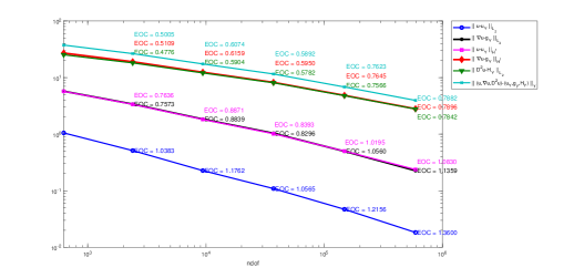
(a) $\mathbb{P}^{1}$ elements

(b) $\mathbb{P}^{2}$ elements

Figure 2. Test problem 5.3. We report the (log–log) error vs. degrees of freedom and the convergence rates for the discrete problem (5.2), applied to a nondivergence form problem (1.1) with domain $\varOmega=\left(-1,1\right)^{2}$, coefficients (5.5) and choosing right hand side $f$ such that
$u(\boldsymbol{x})=x_{1}x_{2}\left({1-\operatorname{e}\!^{1-\left|x_{1}\right|}}\right)\left({1-\operatorname{e}\!^{1-\left|x_{2}\right|}}\right)$.
For $\mathbb{P}^{k}$ elements with both $k=1$ and $2$, we observe optimal convergence rates, that is
${\left\|{u-\mathsf{u}_{\mathbb{X}{}}}\right\|_{\operatorname{H}^{1}(\varOmega)}=\left\|{\nabla{u}-\boldsymbol{\mathsf{g}}{{}_{\mathbb{X}{}}}}\right\|_{\operatorname{H}^{1}(\varOmega)}=\left\|{\operatorname{D}\!^{2}{u}-\boldsymbol{{\mathsf{{H}}}}{{}_{\mathbb{X}{}}}}\right\|_{\operatorname{L}_{2}(\varOmega)}=\operatorname{O}(h^{k}).}$

(a) $\mathbb{P}^{1}$ elements

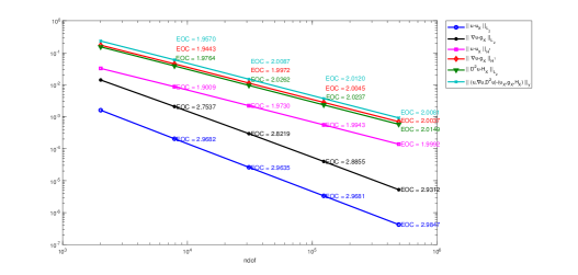
(b) $\mathbb{P}^{2}$ elements

Figure 3. Test problem 5.3. We report the (log–log) error vs. degrees of freedom and the convergence rates for the discrete problem (5.2), applied to a nondivergence form problem (1.1) with domain $\varOmega=\left(-1,1\right)^{2}$, coefficients (5.5) and choosing right hand side $f$ such that
$u(\boldsymbol{x})=x_{1}x_{2}(1-\exp(1-\left|x_{1}\right|))(1-\exp(1-\left|x_{2}\right|))$.
For $\mathbb{P}^{k}$ elements with both $k=1$ and $2$, we observe optimal convergence rates, that is
${\left\|{u-\mathsf{u}_{\mathbb{X}{}}}\right\|_{\operatorname{H}^{1}(\varOmega)}=\left\|{\nabla{u}-\boldsymbol{\mathsf{g}}{{}_{\mathbb{X}{}}}}\right\|_{\operatorname{H}^{1}(\varOmega)}=\left\|{\operatorname{D}\!^{2}{u}-\boldsymbol{{\mathsf{{H}}}}{{}_{\mathbb{X}{}}}}\right\|_{\operatorname{L}_{2}(\varOmega)}=\operatorname{O}(h^{k}).}$

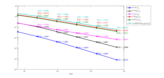
(a) $\mathbb{P}^{1}$ elements

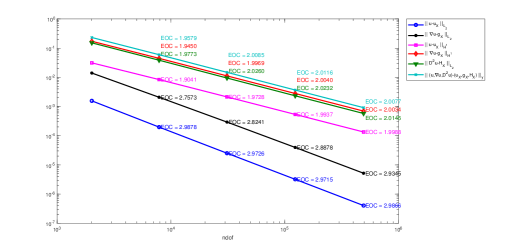
(b) $\mathbb{P}^{2}$ elements

Figure 4. Test problem 5.3. We report the (log–log) error vs. degrees of freedom and the convergence rates for the discrete problem (5.2), applied to a nondivergence form problem (1.1) with domain $\varOmega=\left(-1,1\right)^{2}$, coefficients (5.5) and choosing right hand side $f$ such that
$u(\boldsymbol{x})=x_{1}x_{2}(1-\exp(1-\left|x_{1}\right|))(1-\exp(1-\left|x_{2}\right|))$.
For $\mathbb{P}^{k}$ elements with both $k=1$ and $2$, we observe optimal convergence rates, that is
${\left\|{u-\mathsf{u}_{\mathbb{X}{}}}\right\|_{\operatorname{H}^{1}(\varOmega)}=\left\|{\nabla{u}-\boldsymbol{\mathsf{g}}{{}_{\mathbb{X}{}}}}\right\|_{\operatorname{H}^{1}(\varOmega)}=\left\|{\operatorname{D}\!^{2}{u}-\boldsymbol{{\mathsf{{H}}}}{{}_{\mathbb{X}{}}}}\right\|_{\operatorname{L}_{2}(\varOmega)}=\operatorname{O}(h^{k}).}$

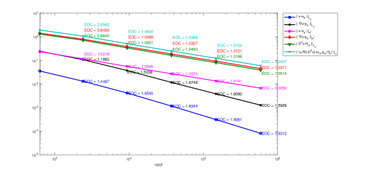
(a) $\mathbb{P}^{1}$ elements

(b) $\mathbb{P}^{2}$ elements

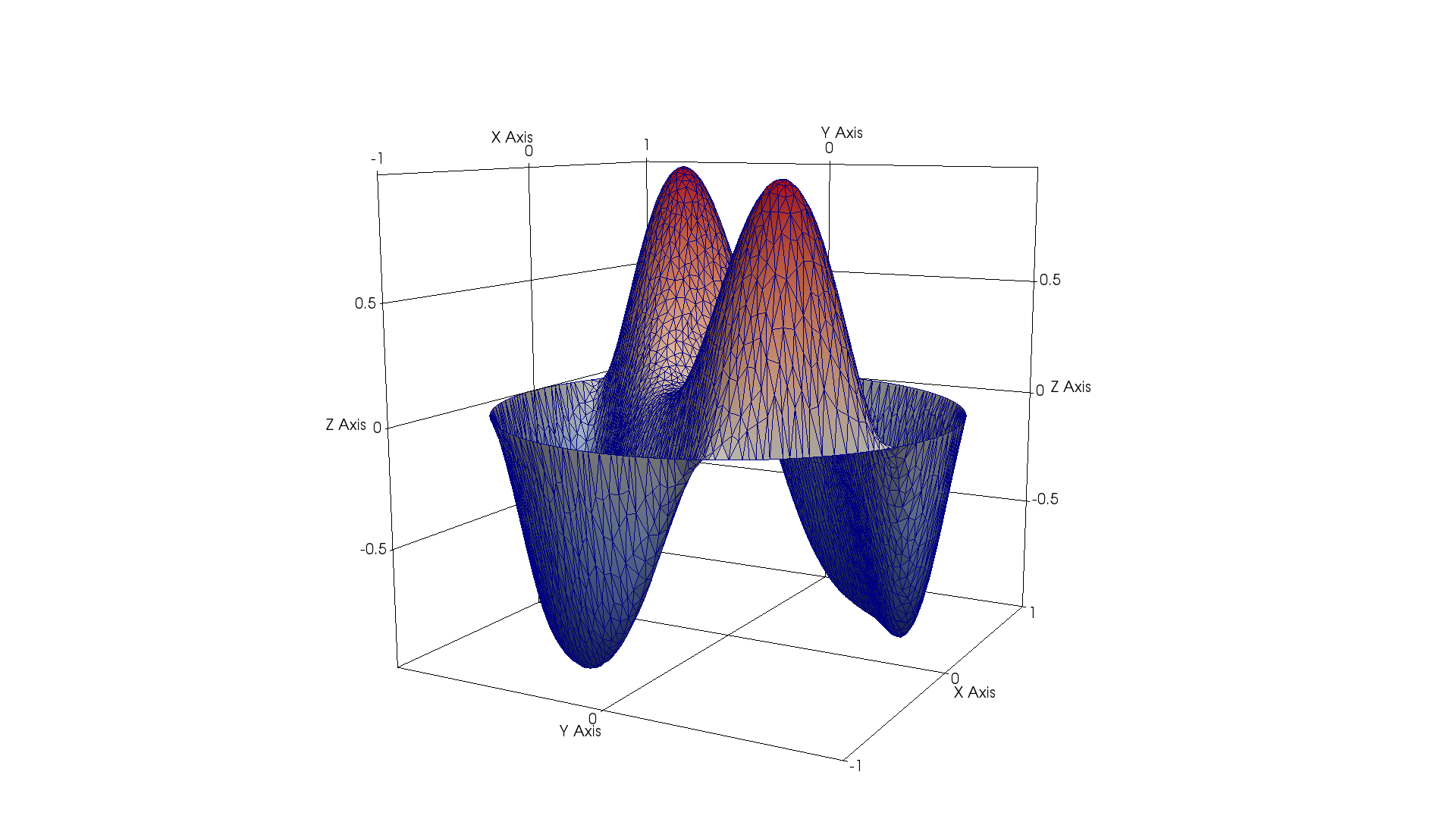
Figure 5. Test problem 5.4. Numerically computed solution via discrete problem (5.2) with $\theta=0.5$ in the unit disk domain with coefficients (5.7) and choosing the forcing $f$ such that
$u(\boldsymbol{x})=\sin(\mathrm{\pi}(x_{1}^{2}+x_{2}^{2}))\cos(\mathrm{\pi}(x_{1}-x_{2})),$
by isoparametric $\mathbb{P}^{2}$-element, $k=2$, and $605973$ degrees of freedom.

Figure 6. Test problem 5.4. We report the (log–log) error vs. degrees of freedom and the convergence rates for the discrete problem (5.2) with $\theta=0.5$, applied to a nondivergence form problem in the unit disk domain, with coefficients (5.7) and choosing the forcing $f$ such that
$u(\boldsymbol{x})=\sin(\mathrm{\pi}(x_{1}^{2}+x_{2}^{2}))\cos(\mathrm{\pi}(x_{1}-x_{2}))$.
For $\mathbb{P}^{k}$ elements with both $k=1$ and $2$, we observe optimal convergence rates, that is ${\left\|{u-\mathsf{u}_{\mathbb{X}{}}}\right\|_{\operatorname{H}^{1}(\varOmega)}=\left\|{\nabla{u}-\boldsymbol{\mathsf{g}}{{}_{\mathbb{X}{}}}}\right\|_{\operatorname{H}^{1}(\varOmega)}=\left\|{\operatorname{D}\!^{2}{u}-\boldsymbol{{\mathsf{{H}}}}{{}_{\mathbb{X}{}}}}\right\|_{\operatorname{L}_{2}(\varOmega)}=\operatorname{O}(h^{k}).}$ For $k=2$, the isoparametric finite element is used.

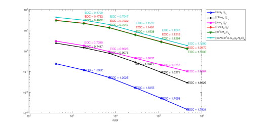
(a) $\mathbb{P}^{1}$ elements

(b) $\mathbb{P}^{2}$ elements

Figure 7. Test problem 5.6. Adaptively refined mesh, generated by Algorithm 4.10 with $\beta=0.3$ and after $8$ iterations, for polynomial degree $k=2$ ( and $122598$ degrees of freedom).

Figure 8. Adaptive mesh refinement Algorithm 4.10 on problem 5.6 with $\mathbb{P}^{1}$ elements. We plot the errors in various norms of the discrete problem (5.2) with $\theta=0.5$ for uniform and adaptive mesh, on the domain $\varOmega=(0,1)\times(0,1)$ with coefficients (5.9) and exact solution
$u(\boldsymbol{x})=x_{1}x_{2}(x_{1}-1)(x_{2}-1)\exp(-1000((x_{1}-0.5)^{2}+(x_{2}-0.117)^{2}))$. Although uniform and adaptive errors seem asymptotically equivalent (because the solution is not really singular), the adaptive error is an order of magnitude smaller.

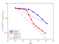
(a) full norm

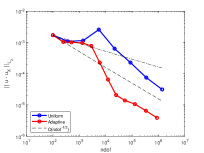
(b) L2 norm

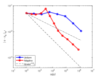
(c) H1 seminorm

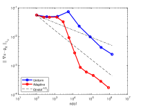
(d) L2 of recovered gradient norm

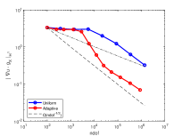
(e) H1 of recovered gradient seminorm

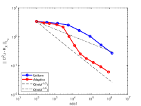
(f) L2 of recovered Hessian norm

Figure 9. Adaptive mesh refinement Algorithm 4.10 on problem 5.6 with $\mathbb{P}^{2}$ elements. We plot the errors in various norms of the discrete problem (5.2) with $\theta=0.5$ for uniform and adaptive mesh, on the domain $\varOmega=(0,1)\times(0,1)$ with coefficients (5.9) and exact solution
$u(\boldsymbol{x})=x_{1}x_{2}(x_{1}-1)(x_{2}-1)\exp(-1000((x_{1}-0.5)^{2}+(x_{2}-0.117)^{2}))$. Compared to 8, also in this case we see that despite their asymptotic equivalence, the adaptive error in all norms becomes an order of magnitude smaller than the uniform error after $8$ iterations. The higher polynomial degree makes this shift more pronounced.

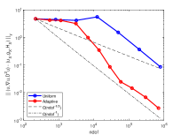
(a) full norm

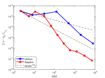
(b) L2 norm

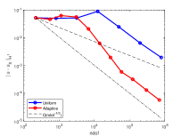
(c) H1 seminorm

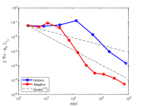
(d) L2 of recovered gradient norm

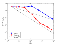
(e) H1 of recovered gradient seminorm

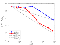
(f) L2 of recovered Hessian norm

Figure 10. Test problem 5.7. Adaptively refined mesh, generated by Algorithm 4.10 with $\beta=0.3$ and after $8$ iterations, for polynomial degree $k=2$ ( and $98679$ degrees of freedom).

Figure 11. Adaptive mesh refinement Algorithm 4.10 on problem 5.7 with $\mathbb{P}^{1}$ elements. We plot the errors in various norms of the discrete problem (5.2) with $\theta=0.5$ for uniform and adaptive mesh, on the domain $\varOmega=(0,1)\times(0,1)$ with coefficients (5.9) and exact solution
Although the performance of $\mathbb{P}^{1}$ elements is not the best, this example shows that the gradient is better approximated in the $\operatorname{H}^{1}(\varOmega)^{2}$ norm.

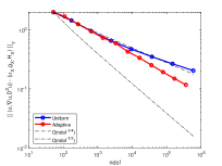
(a) full error norm

(b) L2 error norm

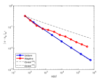
(c) H1 error seminorm

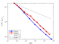
(d) L2 of recovered gradient norm

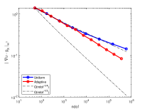
(e) H1 or recovered gradient norm

(f) L2 of recovered Hessian norm

Figure 12. Adaptive mesh refinement Algorithm 4.10 on problem 5.7 with $\mathbb{P}^{2}$ elements. We plot the errors in various norms of the discrete problem (5.2) with $\theta=0.5$ for uniform and adaptive mesh, on the domain $\varOmega=(0,1)\times(0,1)$ with coefficients (5.9) and exact solution
The superiority of the $\mathbb{P}^{2}$ elements in combination with the adaptive method versus the uniform $\mathbb{P}^{2}$ elements is clearly exhibited here, especially in the approximation of the gradient and the Hessian.

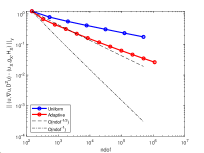
(a) full error norm

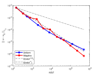
(b) L2 error norm

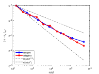
(c) H1 error seminorm

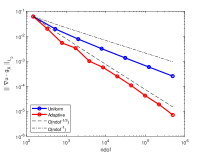
(d) L2 of recovered gradient norm

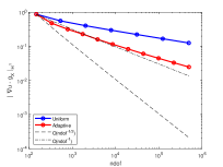
(e) H1 or recovered gradient norm

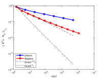
(f) L2 of recovered Hessian norm

References

- Arjmand and Kreiss [2017] D. Arjmand and G. Kreiss. An Equation-Free Approach for Second Order Multiscale Hyperbolic Problems in Non-Divergence Form. online preprint 1708.09446, arXiv, 08 2017. URL https://arxiv.org/abs/1708.09446v2.
- Armstrong and Smart [2010] S. N. Armstrong and C. K. Smart. An easy proof of Jensen’s theorem on the uniqueness of infinity harmonic functions. Calc. Var. Partial Differential Equations, 37(3-4):381–384, 2010. ISSN 0944-2669. doi: 10.1007/s00526-009-0267-9. URL https://arxiv.org/abs/0906.3325v3.
- Aziz et al. [1985] A. K. Aziz, R. B. Kellogg, and A. B. Stephens. Least squares methods for elliptic systems. Mathematics of Computation, 44(169):53–70, 1985. ISSN 0025-5718, 1088-6842. doi: 10.1090/S0025-5718-1985-0771030-5. URL https://www.ams.org/mcom/1985-44-169/S0025-5718-1985-0771030-5/.
- Barles and Souganidis [1991] G. Barles and P. E. Souganidis. Convergence of approximation schemes for fully nonlinear second order equations. Asymptotic Analysis, 4(3):271–283, 1991. doi: 10.3233/ASY-1991-4305. URL https://doi.dx.org/10.3233/ASY-1991-4305.
- Bochev and Gunzburger [2006] P. Bochev and M. Gunzburger. Least-squares finite element methods. In International Congress of Mathematicians. Vol. III, pages 1137–1162. Eur. Math. Soc., Zürich, 2006. URL https://mathscinet.ams.org/mathscinet-getitem?mr=2275722.
- Bramble and Schatz [1970] J. H. Bramble and A. H. Schatz. Rayleigh-Ritz-Galerkin methods for dirichlet’s problem using subspaces without boundary conditions. Communications on Pure and Applied Mathematics, 23(4):653–675, 07 1970. ISSN 0010-3640. doi: 10.1002/cpa.3160230408. URL https://onlinelibrary.wiley.com/doi/abs/10.1002/cpa.3160230408.
- Bramble et al. [1997] J. H. Bramble, R. Lazarov, and J. Pasciak. A least-squares approach based on a discrete minus one inner product for first order systems. Mathematics of Computation, 66(219):935–955, 1997. ISSN 0025-5718, 1088-6842. doi: 10.1090/S0025-5718-97-00848-X. URL https://www.ams.org/mcom/1997-66-219/S0025-5718-97-00848-X/.
- Brenner and Scott [2008] S. C. Brenner and L. R. Scott. The mathematical theory of finite element methods, volume 15 of Texts in Applied Mathematics. Springer-Verlag, New York, third edition, 2008. ISBN 978-0-387-75934-0. doi: 10.1007/978-0-387-75934-0. URL http://www.worldcat.org/oclc/751583766.
- Böhmer [2010] K. Böhmer. Numerical methods for nonlinear elliptic differential equations. Numerical Mathematics and Scientific Computation. Oxford University Press, Oxford, 2010. ISBN 978-0-19-957704-0. doi: 10.1093/acprof:oso/9780199577040.001.0001. URL http://www.worldcat.org/oclc/758731033. A synopsis.
- Caboussat et al. [2013] A. Caboussat, R. Glowinski, and D. C. Sorensen. A least-squares method for the numerical solution of the Dirichlet problem for the elliptic Monge-Ampère equation in dimension two. ESAIM. Control, Optimisation and Calculus of Variations, 19(3):780–810, 2013. ISSN 1292-8119. doi: http://dx.doi.org/10.1051/cocv/2012033. URL 10.1051/cocv/2012033.
- Caffarelli and Cabré [1995] L. A. Caffarelli and X. Cabré. Fully nonlinear elliptic equations, volume 43 of American Mathematical Society Colloquium Publications. American Mathematical Society, Providence, RI, 1995. ISBN 0-8218-0437-5. URL http://www.worldcat.org/oclc/246542992.
- Capdeboscq et al. [2020] Y. Capdeboscq, T. Sprekeler, and E. Süli. Finite element approximation of elliptic homogenization problems in nondivergence-form. ESAIM: Mathematical Modelling and Numerical Analysis, 54(4):1221–1257, July 2020. ISSN 0764-583X, 1290-3841. doi: 10.1051/m2an/2019093. URL https://www.esaim-m2an.org/articles/m2an/abs/2020/04/m2an190116/m2an190116.html.
- Ciarlet [2002] P. G. Ciarlet. The finite element method for elliptic problems, volume 40 of Classics in Applied Mathematics. Society for Industrial and Applied Mathematics, Philadelphia, 2002. ISBN 978-0-89871-514-9. URL http://www.worldcat.org/oclc/985929351. OCLC: 985929351.
- Costabel and Dauge [1999] M. Costabel and M. Dauge. Maxwell and Lamé eigenvalues on polyhedra. Mathematical Methods in the Applied Sciences, 22(3):243–258, 1999. ISSN 0170-4214. doi: 10.1002/(SICI)1099-1476(199902)22:3¡243::AID-MMA37¿3.0.CO;2-0. URL https://perso.univ-rennes1.fr/martin.costabel/publis/CoDaMax_eig.pdf.
- Davydov and Saeed [2013] O. Davydov and A. Saeed. Numerical solution of fully nonlinear elliptic equations by Böhmer’s method. Journal of Computational and Applied Mathematics, 254:43–54, 2013. ISSN 0377-0427. doi: 10.1016/j.cam.2013.03.009. URL http://dx.doi.org/10.1016/j.cam.2013.03.009.
- Dean and Glowinski [2006] E. J. Dean and R. Glowinski. Numerical methods for fully nonlinear elliptic equations of the Monge–Ampère type. Computer Methods in Applied Mechanics and Engineering, 195(13):1344–1386, 02 2006. ISSN 0045-7825. doi: 10.1016/j.cma.2005.05.023. URL http://www.sciencedirect.com/science/article/pii/S0045782505002860.
- Dörfler [1996] W. Dörfler. A convergent adaptive algorithm for Poisson’s equation. SIAM J. Numer. Anal., 33(3):1106–1124, 1996. ISSN 0036-1429. doi: 10.1137/0733054. URL http://dx.doi.org/10.1137/0733054.
- Evans [1985] L. C. Evans. Some Estimates for Nondivergence Structure, Second Order Elliptic Equations. Transactions of the American Mathematical Society, 287(2):701–712, 1985. ISSN 0002-9947. doi: 10.2307/1999671. URL https://www.jstor.org/stable/1999671.
- Evans [2010] L. C. Evans. Partial differential equations, volume 19 of Graduate Studies in Mathematics. American Mathematical Society, Providence, RI, second edition, 2010. ISBN 978-0-8218-4974-3. URL http://www.worldcat.org/oclc/465190110.
- Fabes and Stroock [1983] E. B. Fabes and D. W. Stroock. The Lp-intergrability of Green’s functions andfundamental solutions for elliptic and parabolic equations. online preprint 2486 47, Institute for Mathematics and its Applications, University of Minnesota, 1983. URL http://conservancy.umn.edu/handle/11299/4919. also available as http://hdl.handle.net/11299/4919.
- Feng and Jensen [2017] X. Feng and M. Jensen. Convergent semi-Lagrangian methods for the Monge-Ampère equation on unstructured grids. SIAM Journal on Numerical Analysis, 55(2):691–712, 2017. ISSN 0036-1429. doi: 10.1137/16M1061709. URL https://epubs.siam.org/doi/10.1137/16M1061709.
- Feng et al. [2017] X. Feng, L. Hennings, and M. Neilan. Finite element methods for second order linear elliptic partial differential equations in non-divergence form. Mathematics of Computation, 86(307):2025–2051, 2017. ISSN 0025-5718, 1088-6842. doi: 10.1090/mcom/3168. URL https://www.ams.org/mcom/2017-86-307/S0025-5718-2017-03168-9/.
- Feng et al. [2018] X. Feng, M. Neilan, and S. Schnake. Interior Penalty Discontinuous Galerkin Methods for Second Order Linear Non-divergence Form Elliptic PDEs. Journal of Scientific Computing, 74(3):1651–1676, Mar. 2018. ISSN 1573-7691. doi: 10.1007/s10915-017-0519-3. URL https://link-springer-com.ezproxy.sussex.ac.uk/article/10.1007/s10915-017-0519-3.
- Froese and Oberman [2009] B. D. Froese and A. M. Oberman. Numerical averaging of non-divergence structure elliptic operators. Communications in Mathematical Sciences, 7(4):785–804, 12 2009. ISSN 1539-6746, 1945-0796. URL https://projecteuclid.org/euclid.cms/1264434133.
- Gallistl [2017] D. Gallistl. Variational Formulation and Numerical Analysis of Linear Elliptic Equations in Nondivergence form with Cordes Coefficients. SIAM Journal on Numerical Analysis, 55(2):737–757, 01 2017. ISSN 0036-1429. doi: 10.1137/16M1080495. URL https://epubs-siam-org/doi/10.1137/16M1080495.
- Gallistl [2019] D. Gallistl. Numerical approximation of planar oblique derivative problems in nondivergence form. Mathematics of Computation, 88(317):1091–1119, 2019. ISSN 0025-5718, 1088-6842. doi: 10.1090/mcom/3371. URL https://www.ams.org/mcom/2019-88-317/S0025-5718-2018-03371-3/.
- Gallistl and Süli [2019] D. Gallistl and E. Süli. Mixed Finite Element Approximation of the Hamilton–Jacobi–Bellman Equation with Cordes Coefficients. SIAM Journal on Numerical Analysis, 57(2):592–614, 01 2019. ISSN 0036-1429. doi: 10.1137/18M1192299. URL https://epubs.siam.org/doi/abs/10.1137/18M1192299.
- Kawecki et al. [2018] E. Kawecki, O. Lakkis, and T. Pryer. A finite element method for the monge-ampère equation with transport boundary conditions. online preprint, arxiv, 07 2018. URL http://arxiv.org/abs/1807.03535. arXiv: 1807.03535.
- Lakkis and Mousavi [2020] O. Lakkis and A. Mousavi. A least-squares Galerkin gradient recovery method for fully nonlinear elliptic equations. online preprint 2007.15498, arXiv, 07 2020. URL https://arxiv.org/abs/2007.15498v1. to appear in Proceedings of Enumath 2019.
- Lakkis and Pryer [2011] O. Lakkis and T. Pryer. A finite element method for second order nonvariational elliptic problems. SIAM J. Sci. Comput., 33(2):786–801, 2011. ISSN 1064-8275. doi: 10.1137/100787672. URL https://arxiv.org/abs/1003.0292.
- Lakkis and Pryer [2013] O. Lakkis and T. Pryer. A finite element method for nonlinear elliptic problems. SIAM Journal on Scientific Computing, 35(4):A2025–A2045, 2013. doi: 10.1137/120887655. URL http://arxiv.org/abs/1103.2970.
- Lakkis and Pryer [2015] O. Lakkis and T. Pryer. An adaptive finite element method for the infinity Laplacian. In A. Abdulle, S. Deparis, D. Kressner, F. Nobile, and M. Picasso, editors, Numerical Mathematics and Advanced Applications - ENUMATH 2013, Lecture Notes in Computational Science and Engineering, pages 283–291. Springer International Publishing, Jan. 2015. ISBN 978-3-319-10704-2 978-3-319-10705-9. doi: 10.1007/978-3-319-10705-9˙28. URL http://arxiv.org/abs/1311.3930.
- Logg et al. [2012] A. Logg, K.-A. Mardal, and G. N. Wells. Automated solution of differential equations by the finite element method, volume 84 of Lecture Notes in Computational Science and Engineering. Springer, Heidelberg, 2012. ISBN 978-3-642-23098-1; 978-3-642-23099-8. doi: 10.1007/978-3-642-23099-8. URL http://dx.doi.org/10.1007/978-3-642-23099-8. The FEniCS book.
- Neilan [2014] M. Neilan. Finite element methods for fully nonlinear second order PDEs based on a discrete Hessian with applications to the Monge–Ampère equation. Journal of Computational and Applied Mathematics, 263:351–369, June 2014. ISSN 0377-0427. doi: 10.1016/j.cam.2013.12.027. URL http://www.sciencedirect.com/science/article/pii/S0377042713007000.
- Neilan [2017] M. Neilan. Convergence analysis of a finite element method for second order non-variational elliptic problems. J. Numer. Math., 25(3):169–184, 2017. ISSN 1570-2820. doi: 10.1515/jnma-2016-1017. URL https://doi.org/10.1515/jnma-2016-1017.
- Nochetto and Zhang [2018] R. H. Nochetto and W. Zhang. Discrete ABP estimate and convergence rates for linear elliptic equations in non-divergence form. Foundations of Computational Mathematics, 18(3):537–593, 03 2018. ISSN 1615-3383. doi: 10.1007/s10208-017-9347-y. URL http://dx.doi.org/10.1007/s10208-017-9347-y.
- Smears and Süli [2013] I. Smears and E. Süli. Discontinuous galerkin finite element approximation of nondivergence form elliptic equations with cordès coefficients. SIAM Journal on Numerical Analysis, 51(4):2088–2106, 2013. doi: 10.1137/120899613. URL http://eprints.maths.ox.ac.uk/1623/.
- Smears and Süli [2014] I. Smears and E. Süli. Discontinuous Galerkin finite element approximation of Hamilton-Jacobi-Bellman equations with Cordes coefficients. SIAM J. Numer. Anal., 52(2):993–1016, 2014. ISSN 0036-1429. doi: 10.1137/130909536. URL https://epubs.siam.org/doi/10.1137/130909536.
- Talenti [1965] G. Talenti. Sopra una classe di equazioni ellittiche a coefficienti misurabili. Annali di Matematica Pura ed Applicata, 69(1):285–304, 12 1965. ISSN 1618-1891. doi: 10.1007/BF02414375. URL https://doi.org/10.1007/BF02414375.
- Verfürth [2013] R. Verfürth. A posteriori error estimation techniques for finite element methods. Numerical Mathematics and Scientific Computation. Oxford University Press, Oxford, 2013. ISBN 978-0-19-967942-3. doi: 10.1093/acprof:oso/9780199679423.001.0001. URL http://www.worldcat.org/oclc/5564393801.
- Wang and Wang [2018] C. Wang and J. Wang. A primal-dual weak Galerkin finite element method for second order elliptic equations in non-divergence form. Math. Comp., 87(310):515–545, 2018. ISSN 0025-5718. doi: 10.1090/mcom/3220. URL https://doi.org/10.1090/mcom/3220.