Nucleon axial, tensor, and scalar charges and -terms in lattice QCD
Abstract
We determine the nucleon axial, scalar and tensor charges within lattice Quantum Chromodynamics including all contributions from valence and sea quarks. We analyze three gauge ensembles simulated within the twisted mass formulation at approximately physical value of the pion mass. Two of these ensembles are simulated with two dynamical light quarks and lattice spacing fm and the third with fm includes in addition the strange and charm quarks in the sea. After comparing the results among these three ensembles, we quote as final values our most accurate analysis using the latter ensemble. For the nucleon isovector axial charge we find in agreement with the experimental value. We provide the flavor decomposition of the intrinsic spin carried by quarks in the nucleon obtaining for the up, down, strange and charm quarks , , and , respectively. The corresponding values of the tensor and scalar charges for each quark flavor are also evaluated providing valuable input for experimental searches for beyond the standard model physics. In addition, we extract the nucleon -terms and find for the light quark content MeV and for the strange MeV. The y-parameter that is used in phenomenological studies we find .
pacs:
11.15.Ha, 12.38.Aw, 12.38.Gc, 12.38.-t, 24.85.+pI Introduction
The nucleon axial charge, denoted here by , is a fundamental quantity within the Standard Model (SM) of particle physics. It determines the rate of the weak decay of neutrons into protons and provides a quantitative measure of spontaneous chiral symmetry breaking in hadronic physics. It enters in the analysis of neutrinoless double-beta decay and in the unitarity tests of the Cabibbo-Kobayashi-Maskawa matrix. It is known precisely from neutron beta decay measurements using polarized ultracold neutrons Mendenhall et al. (2013); Mund et al. (2013); Märkisch et al. (2019). Partial conservation of the axial current (PCAC) relates the axial and pseudoscalar charges and allows us to predict the latter. The flavor-diagonal axial charge determines the intrinsic spin carried by the quarks in the nucleon. These are being measured in deep inelastic scattering (DIS) experiments in major facilities such as Jefferson lab and CERN and are targeted in the program of the Electron Ion Collider (EIC).
The isovector tensor and scalar charges can put limits on the existence of beyond SM interactions with scalar and tensor structures Bhattacharya et al. (2012). Ongoing neutrino scattering experiments probing scalar and/or tensor interactions include the experiments DUNE Bischer and Rodejohann (2019), COHERENT Akimov et al. (2017), IsoDAR Abs et al. (2015), LZ Akerib et al. (2015), GEMMA Beda et al. (2012) and the TEXONO collaboration Wong et al. (2007). A review on probing new physics by CP violating processes using the electric dipole moments of atoms can be found in Ref. Yamanaka, N. et al. (2017). High precision measurements of spectral lines in few-electron atoms can probe the existence of exotic forces between electrons Delaunay et al. (2017), while Direct dark matter searches look for new scalar interactions Marrodán Undagoitia and Rauch (2016) and semileptonic kaon Chizhov (1996) or tau Dhargyal (2018) decays experiments are probing for tensor interactions. The tensor and scalar charges are less precisely known, and a determination within lattice QCD can provide essential input for precision measurements probing the existence of novel scalar and tensor interactions aiding experimental searches. The tensor charge is the first Mellin moment of the transversity parton distribution function (PDF) being studied in many experiments including Drell-Yan and semi-inclusive DIS by COMPASS at CERN Adolph et al. (2014) and at Jefferson Lab. The planned SoLID experiment at Jefferson Lab Ye et al. (2017) will allow to measure the tensor charge with an improved accuracy. The extraction of the transversity distribution is less precise than the unpolarized PDF, and additional phenomenological modeling is required. In addition, the flavor-diagonal tensor charge enters into the determination of the quark electric dipole moment contribution to the neutron electric dipole moment Bhattacharya et al. (2016), which signals CP violation.
The nucleon matrix element of the single-flavor scalar operator is directly connected to the quark content of the nucleon, or the so-called nucleon -term, which determines the mass generated by a quark in the nucleon and it is, thus, related to the explicit breaking of chiral symmetry Glashow and Weinberg (1968). Nucleon -terms are relevant for pion and kaon nucleon scattering processes but also for the interpretation of direct-detection dark matter searches. The dark matter candidates under consideration are weakly interacting massive particles in a number of beyond the SM theories that interact with normal matter by elastic scattering with nuclei. Besides its direct relation to the -term, the isovector scalar charge measures the proportionality constant between the neutron-proton mass splitting and the up and down quark mass splitting in the absence of electromagnetism via the relation González-Alonso and Martin Camalich (2014). This relation first appeared in Ref. Gasser and Leutwyler (1982), while a similar result was derived in Ref. Crewther et al. (1979). The fundamental role of these quantities in the physics of weak interactions and in beyond the SM physics makes their non-perturbative determination of central importance.
The non-perturbative nature of the fundamental theory of the strong interaction makes a theoretical calculation of these fundamental quantities difficult. The discretized version of the theory defined on a four-dimensional Euclidean lattice and known as lattice Quantum Chromodynamics (QCD) provides a rigorous, non-perturbative formulation that allows for a numerical simulation with controlled systematic uncertainties. Since, as mentioned already, is accurately measured experimentally it serves as a benchmark quantity for lattice QCD. Numerous past lattice QCD studies Lin et al. (2018a) underestimated and impeded reliable predictions of the other nucleon charges. It is only recently that an accurate computation of was presented Chang et al. (2018) that reproduced the experimental value. It was, however, obtained using chiral extrapolations involving ensembles with heavier than physical pions. For a complete list of lattice QCD results with details on the lattice QCD framework used, we refer to the recent FLAG report Aoki et al. (2019). Reproducing the value of within a lattice QCD framework serves both as a validation and as a most valuable benchmark computation for the extraction of the isovector scalar and tensor charges. In addition, a precise computation of in lattice QCD can provide a constraint for non-standard right-handed currents Bhattacharya et al. (2012).
In this work, we compute the nucleon charges and -terms using gauge configurations generated with the physical values of the light quark masses, avoiding chiral extrapolation or any modeling of the pion mass dependence. We consider two ensembles with two light quarks in the sea, denoted by ensembles, and one ensemble where, besides the light quarks, we include the strange and charm quarks in the sea, denoted with . The latter ensemble provides one of the best description of the QCD vacuum to date and thus we devote most of our computational resources to its analysis and use it to extract our final values. For this ensemble we achieve high precision not only for the isovector axial (A), tensor (T) and scalar (S) quantities but also for the single flavor charges and -terms. Such an accurate computation from first principles of the axial, scalar and tensor charges for each quark flavor, as well as the direct determination of the , strange and charm -terms, constitutes a major step in our understanding of the structure of the nucleon.
The remainder of this paper is organized as follows: in Section II we provide the methodology used for extracting the nucleon charges using lattice QCD, in Section III we detail the analysis carried out, in particular as regards ensuring suppression of excited states, and provide unremormalized results of the nucleon charges. In Section IV we describe our renormalization procedure and in Section V we provide renormalized results for the nucleon charges and compare with phenomenology and other lattice results. In Section VI we review our final results and provide our conclusions.
II Methodology
The axial, tensor and scalar flavor charges are obtained from the nucleon matrix elements of the axial, tensor and scalar operators at zero momentum transfer, given by
| (1) |
where is the nucleon spinor, denotes the quark flavor, and for the axial-vector operator, for the scalar and for the tensor. The renormalization group invariant -term is defined by where is the quark mass.
II.1 Lattice QCD formulation and gauge ensembles
We use three gauge ensembles simulated with a physical value of the pion mass Abdel-Rehim et al. (2017); Alexandrou et al. (2018a) using the twisted mass fermion discretization scheme Frezzotti et al. (2001); Frezzotti and Rossi (2004) with a clover-term Sheikholeslami and Wohlert (1985). The parameters are listed in Table 1. We refer to these ensembles as physical point ensembles. Twisted mass fermions (TMF) provide an attractive formulation for lattice QCD allowing for automatic improvement Frezzotti and Rossi (2004), where is the lattice spacing. This is an important property for evaluating the quantities considered here, since all quantities have lattice artifacts of and are closer to the continuum limit as observed in previous studies using simulation with larger than physical pion mass Alexandrou et al. (2011). A clover-term is added to the TMF action to allow for smaller breaking effects between the neutral and charged pions that lead to the stabilization of simulations with light quark masses close to the physical pion mass. For more details on the TMF formulation see Refs. Frezzotti et al. (2006); Boucaud et al. (2008) and for the simulation strategy Refs. Abdel-Rehim et al. (2017); Alexandrou et al. (2018a).
| Ensemble | [MeV] | L [fm] | |||
|---|---|---|---|---|---|
| , , fm | |||||
| cA2.09.48 | 7.15(2) | 2.98 | 130.3(4)(2) | 4.50(1) | |
| cA2.09.64 | 7.14(4) | 3.97 | 130.6(4)(2) | 6.00(2) | |
| , , fm | |||||
| cB211.072.64 | 6.74(3) | 3.62 | 139.3(7) | 5.12(3) | |
The two ensembles denoted by cA2.09.48 and cA2.09.64, are generated with two dynamical mass degenerate up and down quarks () with mass tuned to reproduce the physical pion mass Abdel-Rehim et al. (2017). They have the same lattice spacing but use two lattice sizes of and allowing for checking finite volume dependence. The ensemble denoted by cB211.072.64 has been generated on a lattice of size with two degenerate light quarks and the strange and charm quarks (+1+1) in the sea with masses tuned to produce the physical pion, kaon and -meson mass, respectively, keeping the ratio of charm to strange quark mass Aoki et al. (2019). For the valence strange and charm quarks we use Osterwalder-Seiler fermions Osterwalder and Seiler (1978) with mass tuned to reproduce the and the baryons Alexandrou and Kallidonis (2017), respectively. Results for nucleon charges using the cA2.09.48 ensemble have been presented in Refs. Alexandrou et al. (2017a, b, c). Since we perform a reanalysis to match our analysis strategy for the cB211.072.64 ensemble, the results are updated.
II.2 Computation of correlators
The nucleon matrix elements are extracted by computing appropriately defined three-point correlators , as well as the nucleon two-point correlators, , at zero momentum. These correlation functions are constructed by creating a state from the vacuum with the quantum numbers of the nucleon at some initial time (source) that is annihilated at a later time (sink), where we take the source time to be zero. All expressions that follow are given in Euclidean space. We consider three-point correlators
| (2) |
where is a local current operator that couples to a quark at insertion time having . is a projector acting on spin indices, and we will use either the so-called unpolarized projector or the three polarized combinations. For , we use the standard nucleon interpolating operator,
| (3) |
where and are up- and down-quark spinors and is the charge conjugation matrix. The local current operator is given by
| (4) |
where is a quark spinor of flavor and the matrices are defined in Eq. (1).
Inserting two complete sets of states in Eq. (2), one obtains a tower of hadron matrix elements with the quantum numbers of the nucleon multiplied by overlap terms and time dependent exponentials. For large enough time separations, the excited state contributions are suppressed compared to the nucleon ground state and one can then extract the desired matrix element. Knowledge of two-point functions is required in order to cancel time dependent exponentials and overlaps. They are given by
| (5) |
In order to increase the overlap of the interpolating operator with the nucleon state and thus decrease overlap with excited states we use Gaussian smeared quark fields via Alexandrou et al. (1994); Gusken (1990):
| (6) | ||||
| (7) |
with APE-smearing Albanese et al. (1987) applied to the gauge fields entering the Gaussian smearing hopping matrix . For the APE smearing Albanese et al. (1987) we use 50 iteration steps and . The Gaussian smearing parameters are tuned to yield approximately a root mean square radius for the nucleon of about 0.5 fm, which has been found to yield early convergence to the nucleon two-point functions. This can be achieved by a combination of the smearing parameters and . We use =0.2, 0.2, and 4.0 and =125, 90, and 50 for ensembles cB211.072.64, cA2.09.64, and cA2.09.48, respectively. We employ a multi-grid solver Frommer et al. (2014) to speed up the inversions that has been extended to the case of the twisted mass operator and shown to yield a speed-up of more than one order of magnitude at the physical point compared to the conjugate gradient method (CG) Alexandrou et al. (2016). The resulting propagators are used to construct two- and three-point correlators.
II.3 Connected and disconnected contributions
The three-point correlators receive two contributions, one arising when the current couples to a valence quark and one when coupled to a sea quark. The former is referred to as giving rise to a connected and the latter to a disconnected contribution. The connected contributions are evaluated using sequential inversions through the sink. Since in this method and the four spin projection matrices needed for the extraction of the charges are fixed, four sets of sequential inversions are performed for each value of in the rest frame of the nucleon. In Table 2 we give the statistics used for computing the connected contributions for the three ensembles analyzed. As can be seen, the statistics are increased as we increase to keep statistical errors comparable for all time separations . Ensemble cB211.072.64 has the largest statistics and we will thus base our final values on this ensembles.
| 8 | 10 | 12 | 14 | 16 | 18 | 20 | |
|---|---|---|---|---|---|---|---|
| [fm] | 0.75 | 0.94 | 1.13 | 1.31 | 1.50 | 1.69 | 1.88 |
| cA2.09.48 | – | 9264 | 9264 | 9264 | 47696 | 69784 | – |
| cA2.09.64 | – | – | 5328 | 8064 | 17008 | – | – |
| [fm] | 0.64 | 0.80 | 0.96 | 1.12 | 1.28 | 1.44 | 1.60 |
| cB211.072.64 | 750 | 1500 | 3000 | 4500 | 12000 | 36000 | 48000 |
For the disconnected contributions we utilize a combination of methods that are suitable for physical point ensembles Alexandrou et al. (2018b). These employ full dilution in spin and color in order to eliminate exactly any contamination from off-diagonal elements and a partial dilution in space-time using Hierarchical Probing Stathopoulos et al. (2013) up to a distance of lattice units taking advantage of the exponential decay of off-diagonal elements with the distance. For the up and down quarks this exponential decay is slow and therefore we combine with deflation of the low modes. For the strange and charm quarks deflation is not necessary due to the heavier mass and we use a distance of and lattice units, respectively, in the Hierarchical Probing. Additionally, we employ the so-called one-end trick Michael and Urbach (2007); McNeile and Michael (2006) that makes use of the properties of the twisted mass action to improve the signal-to-noise ratio. Deflation of low modes and Hierarchical Probing have been employed only for the computations using the cB211.072.64 ensemble. For the cA2.09.48 ensemble we use stochastic sources. In Table 3 we list the parameters and statistics used in the calculation of the disconnected contributions.
| cA2.09.48 | 848000 | 4808250 | 2204672 | 2691250 |
|---|---|---|---|---|
| cB211.072.64 | 600000 | 750x512 | 750x512 | 9000x32 |
| + deflation |
III Analysis of correlators
The nucleon charges can be extracted by taking a ratio of and (c.f. Eqs. (2) and (5)),
| (8) |
where is the energy gap between the ground and first excited states. This ratio becomes time independent for large values of and yielding a plateau, the value of which gives the desired nucleon charge, . In practice, cannot be chosen arbitrarily large because the statistical errors grow exponentially with . Thus, we need to use the smallest that ensures convergence to the nucleon state. In this work, we use several values of and increase the statistics as we increase to keep the statistical error approximately constant, which is essential to reliably assess excited states Alexandrou et al. (2017a); von Hippel et al. (2017). In Table 2 we give the values of used for the connected contribution and the associated statistics. A careful analysis is then performed, employing different methods to study ground state convergence.
When fitting, we carry out correlated fits to the data, i.e. we compute the covariance matrix between jackknife or bootstrap samples and minimize
| (9) |
where are the lattice data, is the fit function, which depends on and . are the values of and/or at which is evaluated and is a vector of the parameters being fitted for.
III.1 Plateau method
We fit the ratio of Eq. (8) to a constant in an interval . This assumes the ground state is the dominant contribution. We choose such that a constant fit describes well the data. The fits are performed independently for each using the same and thus we fit only the data for which satisfies . We seek convergence of the fitted value as increases. An example of this analysis, which we will refer to as the plateau method, is shown in Fig. 1, applied to the isovector axial charge, where we take . As can be seen, as we increase the ratio increases, indicating a convergence only for the two largest time separations. However, the errors also increase and make it difficult to judge convergence.
III.2 Two- and three-state fit
In the two- and three-state fit approaches, we take into account the contributions of the first and second excited states, respectively, using multiple values of and fit them simultaneously. The two-point correlator is described by the tower of states,
| (10) |
where is the nucleon mass and for are excited states with increasing energies. The amplitudes are positive numbers. In our two- and three-state fit analysis we fit the two-point functions using Eq. (10) with, in the first case, and and having four fit parameters and, in the latter case, and and having six fit parameters.
The three-point function correlator is described by the tower of states,
| (11) |
where are matrix elements and overlaps and . When we fit the three-point function with Eq. (11), we use the nucleon mass and the energies of the first and second excited states as obtained from the fit of the two-point functions of Eq. (10) and fit for the amplitudes . The nucleon mass and energies are extracted via a jack-knife analysis from the two-point functions and the resampled values are subsequently used in the jack-knife analysis of the three-point functions. Within such an approach all the nucleon matrix elements share the same set of energies and we restrict the search-space of the fit to the three-point function to the amplitudes only. This means that in the case of the two-state fit analysis and using Eq. (11) with and 1, we have three additional fit parameters to determine. For the three-state fit analysis we have and and six additional fit parameters.
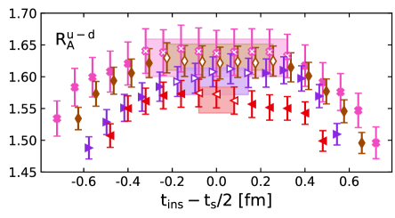
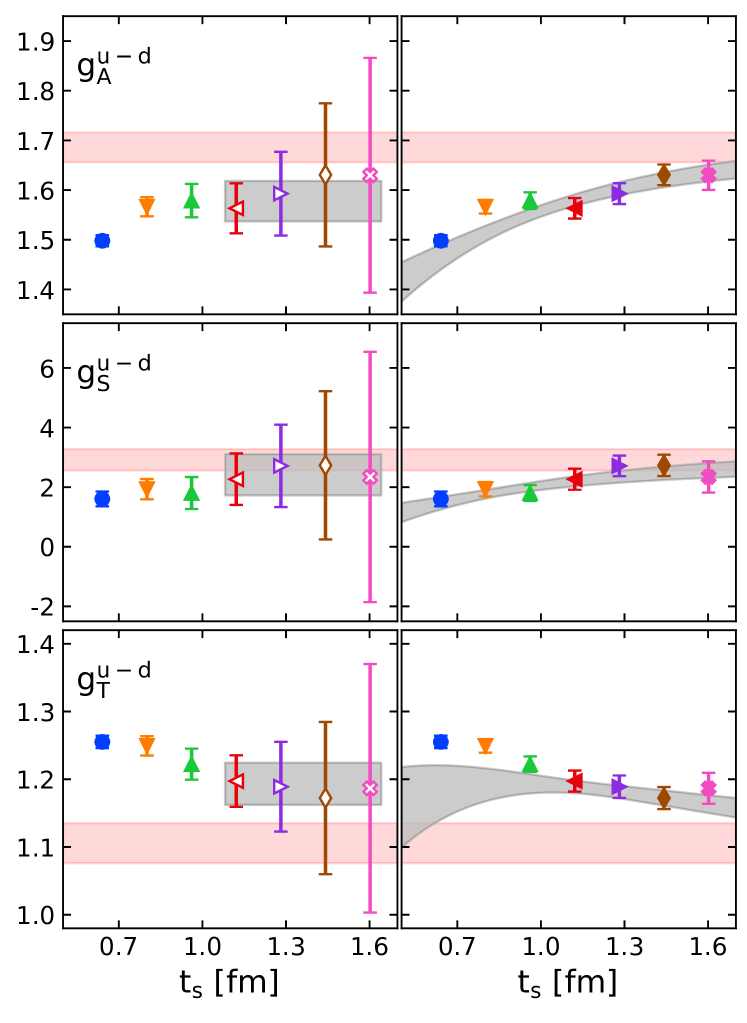
We demonstrate the application of the two- and three-state fit approaches in the case of the axial charge for the cB211.072.64 ensemble. We show in Fig. 2 the ratio for each value of with the predicted curve from two-state fit obtained by fitting two- and three-point functions as described above. The extracted value of is shown with a gray band and the predicted curve for each is shown with a band of the same color as the points. Since we fit two-point functions with the largest statistic available, i.e. obtained by averaging forward, backward, neutron and proton nucleon correlators over 264 source positions per configuration, the ratios shown in Fig. 2 are constructed by dividing the three-point functions by the two-point function with the maximum statistics. This differs from the ratio used in the analysis of the plateau averages where we divide the three-point function by the two-point function having the same statistics as the three point function to take advantage of the correlations between them.
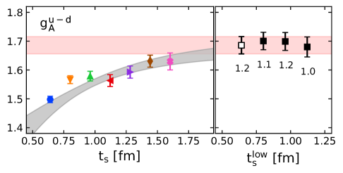
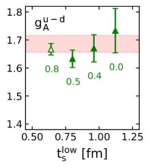
In Fig. 3 we show the resulting curve using the parameters determined from the two-state fit as a function of fixing in Eq. (8). We also show for each the extracted plateau value extracted, following the procedure explained in connection to Fig. 1. For we show the mid point of the ratio since no fit is performed. As can be seen, the two-state fit predicts well the behavior of the ratio and demonstrates that the asymptotic value is reached for values of larger than 2 fm, which is in agreement with the chiral perturbation analysis of Ref. Bar (2019). Therefore, taking the plateau value for the largest considered, which, within errors, seems to have converged, underestimates . In particular, notice that since data are correlated, one might mistake convergence in the window of , which will lead to a small value of . This is why it is important to have precise data for larger time separations. In the right panel of Fig. 3 we show the extracted value of as a function of , i.e. the smallest included in the two-state fit. As can be seen, the values remain consistent as increases. We also give for each point the as given in Eq.(9) that is close to unity for all the cases. We note that the is computed from the fit of the three-point function correlator and the quality of the fit can be better understood by looking at the curves depicted in Fig. 2 than how well the gray band describes the plateau averages in Fig. 3, which are not fitted. Since the values show convergence as increases we select the value obtained by using fm. As we will see below, this will be also in agreement with the three-state fit and the summation method and thus will fulfill our criterion for selecting the two-state fit value that also agrees with the value extracted from the summation method.
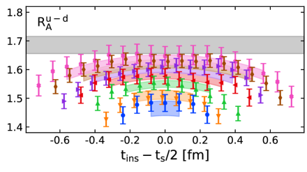
A similar analysis is performed for the three-state fit approach, i.e. when two excited states are considered taking and in Eqs. (10) and (11). The results are given in Fig. 4 where we use the same convention as for the two state-fit and for comparison we show with a red band the errors related to the selected two-state fit value.
III.3 Summation method
We sum over the insertion time in the ratio in Eq. (8) assuming only the lowest state dominates to obtain a linear dependence on , given by
| (12) |
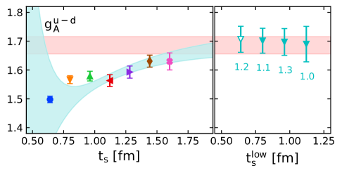
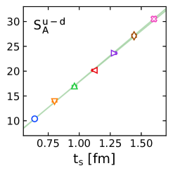
where in the sum we omit the source and sink time slices. The slope extracted from a linear fit to Eq. (12) gives the nucleon charge in the limit of large . By increasing the lowest value of used in the fit we look for convergence in the extracted slope. The advantage of the summation method is that, despite the fact that it still assumes a single state dominance, the excited states are suppressed exponentially with respect to instead of that enters in the plateau method Capitani et al. (2012). On the other hand, the errors tend to be larger since we have two parameters to fit. As an example we show in Fig. 5 the results after applying the summation approach for the case of the isovector axial charge using the cB211.072.64 ensemble. We select as our final value the one extracted from the two-state fit when excited states are detected, since the two-state fit models the data better than either the plateau or the summation method in these cases. Even though the statistical error on the extracted value of the charges is larger than that extracted using the summation method, we prefer to be conservative so that we do not underestimate errors.
III.4 Analysis of the cB211.072.64 ensemble
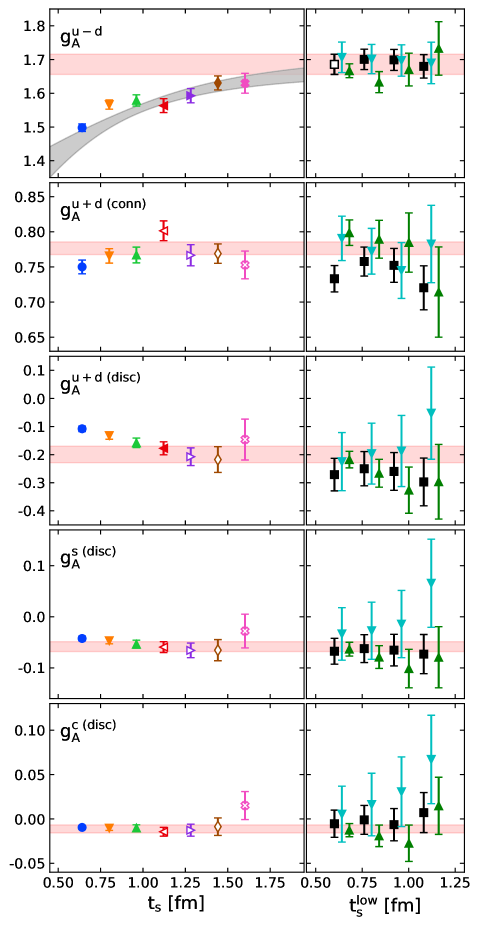
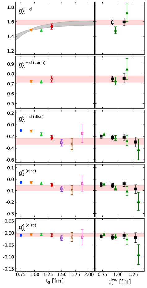
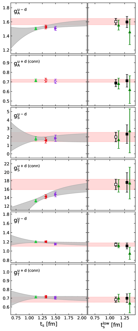
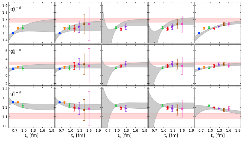
In Fig. 6 we show a comparison among the three aforementioned analysis methods for the axial charges using the cB211.072.64 ensemble. As already observed, the value extracted for the axial charge from the two-state fit shows very mild dependence on the used in the fits. In addition, the value extracted from the two-state fit is confirmed by the three-state fits as well as by the summation method. Therefore, we take as our final result the value extracted from the two-state fit for which and there is agreement with the summation method. The connected and the disconnected parts of the isoscalar charge as well as the strange and charm disconnected contributions do not suffer from large excited states contamination, as can be seen in Fig. 6 by the fact that the plateau results at the largest three or four values of are roughly constant. Furthermore, the plateau values converge to a value that is in agreement with the values extracted using two- and three-state fits and the summation methods and we thus take the weighted average. We note that we follow this procedure for all cases where such a behavior is observed, i.e we take the correlated average of the plateau values for the range of for which these have converged.
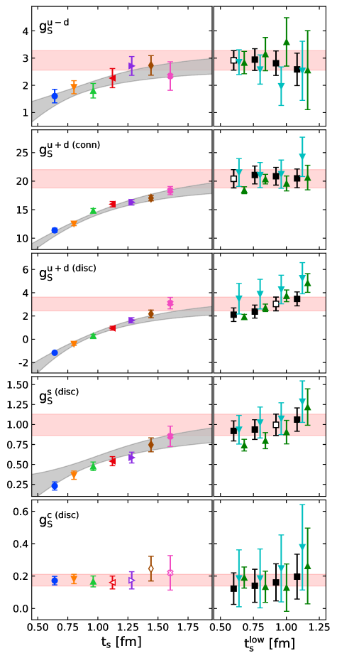
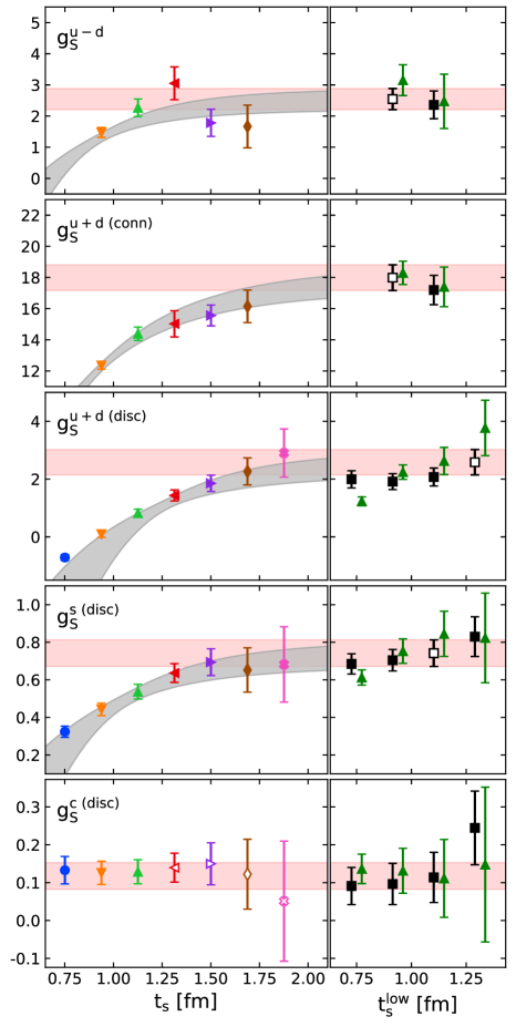
We perform the same analysis for the scalar charge and we show the results in Fig. 7. Contrary to the axial charge, all the contributions to the scalar charges, except for the charm disconnected component, suffer from large excited states contamination. As can be seen, the plateau values show a similar behavior as showing convergence of the two-state fit at larger than 2 fm. We therefore choose as our final value the one extracted from the two-state fit when it agrees with the summation method and does not show dependence on . We thus use fm in the fit of the isovector , connected isoscalar and the strange disconnected scalar charge . For the disconnected isoscalar scalar charge and , we use a larger value fm to better account for the upward trend still present in the data. We note that the results on the scalar charges have errors about ten times larger as compared to the axial charges.
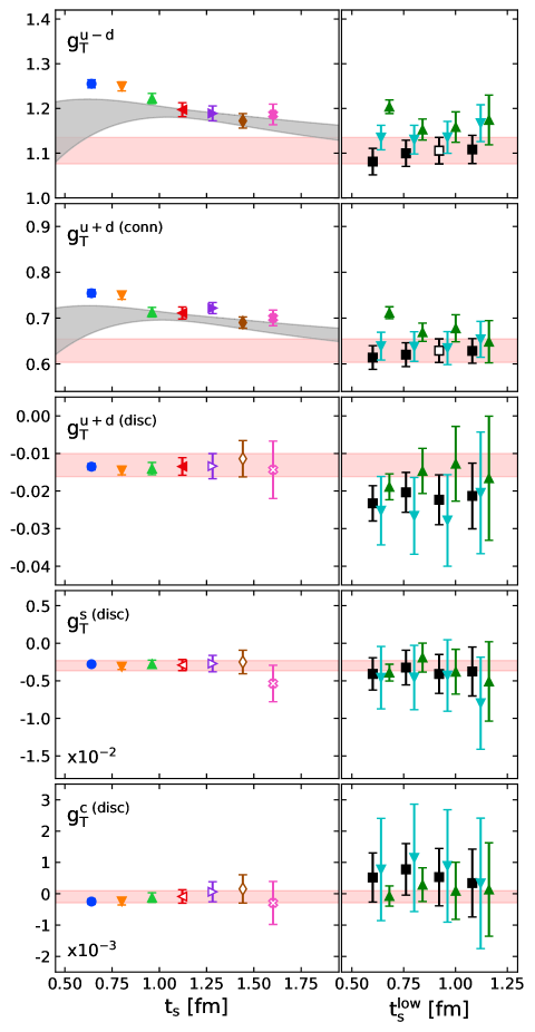
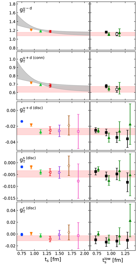
We perform the same analysis for the tensor charges and show the resulting values in Fig. 8. As can be seen, for the isovector and connected isoscalar tensor charge , there is no agreement between the two-state and summation values for smaller values. The value from the two-state fit becomes consistent with the one extracted from the summation when fm and this is what we select as final value. This demonstrates that the larger values of are crucial for properly probing ground state dominance.
The results for the connected isoscalar charge are shown in Fig. 8. As can be seen, the plateau values computed by fitting to a constant using the data at and fm are compatible and one may think that the values have converged. However, both the results from the two-state and three-state fits are lower. Furthermore, there is a tension between the two-state fit and the summation method for fm and only when fm that they become consistent. This would correspond to about 2.6 fm in the plateau method. This again demonstrates the importance of having precise data for large values.
Similarly to the axial charge, the disconnected contributions do not show large effects from excited states. We thus take the average of the plateau values for the range of for which these have converged as the final value.
| (conn) | (disc) | ||||
|---|---|---|---|---|---|
| 1.686(30) | 0.7766(90) | -0.199(29) | -0.0583(96) | -0.0112(45) | |
| 3.04(59) | 20.4(1.6) | 3.04(59) | 1.00(13) | 0.175(36) | |
| 1.106(32) | 0.629(27) | -0.0131(31) | -0.00299(68) | -0.00010(19) |
We summarize in Table 4 the bare values for the isovector, connected and disconnected isoscalar, strange and charm axial, scalar and tensor charges. These results clearly demonstrate that disconnected contributions cannot be neglected at the physical point. They are enhanced in comparison to the values obtained at heavier pion masses where for example the disconnected part of using a ensemble simulated at a pion mass of MeV was -0.07(1) Abdel-Rehim et al. (2014) as compared to -0.199(29) for the cB211.072.64 ensemble.
III.5 Analysis of cA2.09.48
We repeat the same analysis described for the cB211.072.64 ensemble for the cA2.09.48 ensemble. Since we now use correlated fits the values presented in Refs. Alexandrou et al. (2017a, b) are modified but remain within their statistical errors. For the connected components on this ensemble we have only three values of for the matrix element of the axial and tensor currents determining and and five for the scalar current determining . The three smaller values of have constant statistics, as shown in Table 2, and thus their statistical errors increase significantly with increasing . This means that the quality of the fits are not as good as for the cB211.072.64 ensemble. In particular, a three-state fit analysis cannot be performed due to the low statistics and the small number of . On the other hand the disconnected contributions are available for a larger number of and we thus show a more complete analysis. The results of the analysis are summarized in Fig. 9 for the axial charges, in Fig. 10 for the scalar charges and in Fig. 11 for the tensor charges. For the connected matrix elements of the axial and scalar current the two-state fit with fm agrees with the summation value as well as with the value extracted when using fm and thus we take it as final value. On the other hand the tensor charge shows a more severe contamination of excited states and, similarly to the cB211.072.64 ensemble, we take as final value the two-state fit result at larger separation, namely fm. Disconnected contributions to axial and tensor charges show very mild excited state contamination and we take the plateaus average as final value. On the hand for the scalar charge excited states are more severe and we take the two-state fit result at fm for the disconnected isoscalar and fm for the strange disconnected . We summarize in Table 5 the bare values for the isovector, connected and disconnected isoscalar, strange and charm axial, scalar and tensor charges for this ensemble.
| (conn) | (disc) | ||||
|---|---|---|---|---|---|
| 1.590(35) | 0.747(32) | -0.284(53) | -0.077(22) | -0.0082(64) | |
| 2.54(34) | 17.99(82) | 2.59(44) | 0.742(71) | 0.118(35) | |
| 1.116(40) | 0.638(35) | -0.0268(42) | -0.0048(14) | -0.0071(44) |
III.6 Analysis of cA2.09.64
For the cA2.09.64 ensemble we only have three values of and therefore the analysis of excited states is again not as accurate as for the cB211.072.64 ensemble. In addition we only have connected contributions since the purpose of the analysis of the cA2.09.64 ensemble is to check for finite volume effects using the connected contributions which are much more precise and less expensive. Following the same analysis procedure we summarize the results on the isovector and connected isoscalar charges in Fig 12. Given that the values for the two available are consistent between them and with the values from the summation, we take as our selected values the ones extracted from the two state fits when using . We remark that while for scalar charge the plateau values show convergence we know from the more accurate analysis using the cB211.072.64 ensemble that this quantity has non-negligible contribution from excited states and thus we still fit it using a two-state fit. If we were to extract it using the weighted average plateau values we would obtain a value that is compatible with that from the two-state fit with however a smaller error. We therefore conservatively quote the value with the larger statistical error.
We summarize in Table 6 the bare values for the isovector and connected isoscalar axial, scalar and tensor charges that can be directly compared to the values listed in Table 5 for the cA2.09.48 ensemble, since these ensembles have the same renormalization constants. The results obtained using the cA2.09.48 and cA2.09.64 are compatible indicating that finite size effects are within our statistical accuracy.
| (conn) | ||
|---|---|---|
| 1.603(45) | 0.711(16) | |
| 1.99(56) | 17.1(1.2) | |
| 1.139(38) | 0.683(30) |
IV Renormalization
Lattice QCD matrix elements must be renormalized to extract physical quantities. We use the scheme Martinelli et al. (1995) to compute non-perturbatively the renormalization functions using the momentum source method Gockeler et al. (1999). We implement it as done in Ref. Alexandrou et al. (2012) and remove lattice spacing effects by subtracting terms computed in perturbation theory Constantinou et al. (2009); Alexandrou et al. (2017d). We distinguish between non-singlet and singlet renormalization functions, where for the latter we compute, in addition to the connected, the disconnected contributions. The non-singlet and singlet renormalization functions , and for the ensemble cB211.072.64 are computed using ensembles simulated at the same value and at five values of the pion mass so the chiral limit can be taken. The parameters for these ensembles are given in Table 7. For the renormalization of the matrix elements using the cA2.09.48 and cA2.09.64 ensembles we have analyzed ensembles as extensively discussed in Ref. Alexandrou et al. (2017d). The scalar quantities are renormalized with the pseudo-scalar renormalization constant, , since they are computed using the pseudo-scalar current in the twisted-mass formulation.
| , fm | ||
|---|---|---|
| lattice size | ||
| 0.0060 | 0.14836 | |
| 0.0075 | 0.17287 | |
| 0.0088 | 0.18556 | |
| 0.0100 | 0.19635 | |
| 0.0115 | 0.21028 |
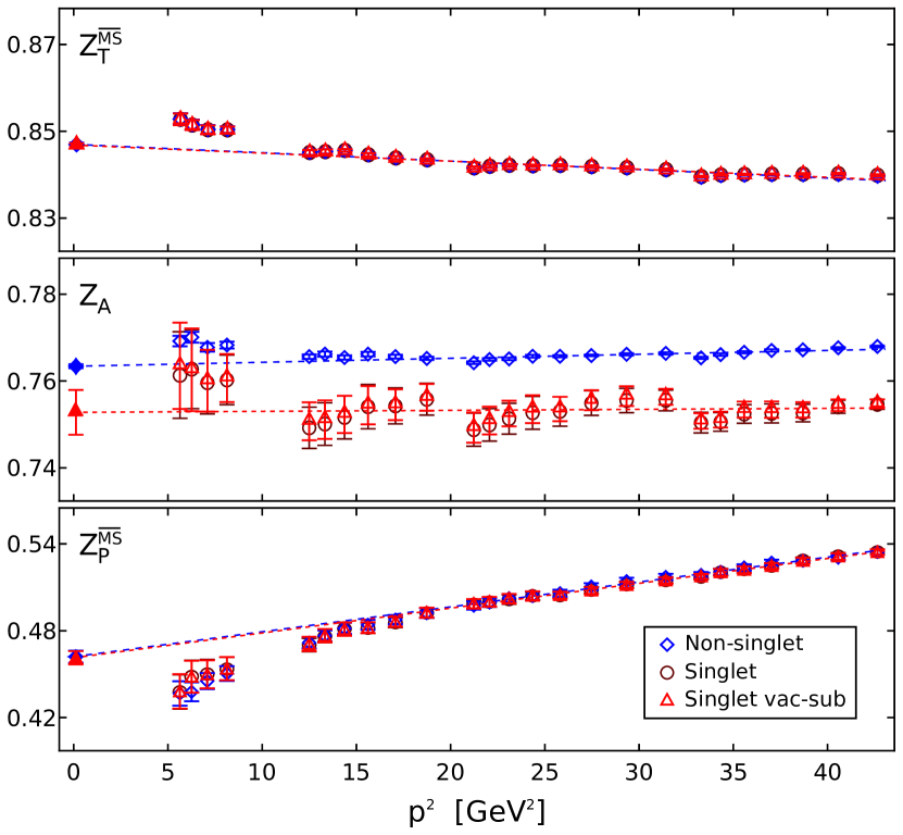
We show in Fig. 13 the determination of the non-singlet and singlet , and renormalization constants for the ensemble cB211.072.64. The mass dependence is mild and we extrapolate to the chiral limit using the results at the five values of the twisted mass parameters.
The values of the renormalization functions are listed in Table 8. The renormalization functions were computed in Refs. Alexandrou et al. (2017a, b) and are included here for easy reference. We estimate the systematic error by varying the fit ranges used for the extrapolation of the scale . While the renormalization function for the axial current is scheme and scale independent, the corresponding ones for the scalar and tensor charges, and , are scale and scheme-dependent and are given in the scheme at 2 GeV. The singlet and non-singlet renormalization functions are different only for . For we use the conversion factor calculated to 2-loops in perturbation theory Skouroupathis and Panagopoulos (2009). The conversion factor for and is the same as in the corresponding non-singlet case.
| =2 | 0.7910(6) | 0.797(9) | 0.50(3) | 0.50(2) | 0.855(2) | 0.852(5) |
|---|---|---|---|---|---|---|
| =4 | 0.763(1) | 0.753(5) | 0.462(4) | 0.461(5) | 0.847(1) | 0.846(1) |
V Results
V.1 Nucleon charges
In Table 9 we present our final renormalized values for the isovector charges for the three ensembles. Comparing the values extracted from the two ensembles with and no volume effects can be resolved within our statistical accuracy. This corroborates our previous results at heavier than physical pion masses where no volume effects were detected for Alexandrou et al. (2011). A previous study of cut-off effects using three ensembles with lattice spacings , 0.070(4), and 0.056(4) fm, revealed that cut-off effects are negligible for a range of pion masses spanning 260 MeV to 450 MeV Alexandrou et al. (2011) for our twisted mass action. Having a clover term we expect cut-off effects to be reduced and be within our current accuracy. However, we are planing to repeat the analysis for two further ensembles with smaller lattice spacings that will enable us to take the proper continuum limit at the physical point.
| cA2.09.48 | 1.258(27) | 1.27(19) | 0.954(35) |
|---|---|---|---|
| cA2.09.64 | 1.268(36) | 0.99(28) | 0.974(33) |
| cB211.072.64 | 1.286(23) | 1.35(17) | 0.939(27) |
| 0.817(29) | -0.450(29) | -0.061(17) | -0.0065(51) | |
| 5.78(32) | 4.51(32) | 0.371(38) | 0.059(18) | |
| 0.737(23) | -0.217(23) | -0.0041(12) | -0.0060(37) |
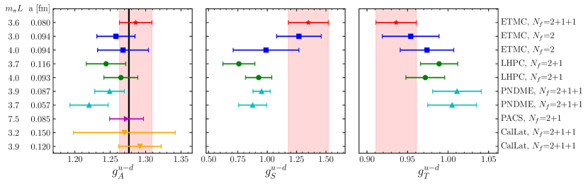
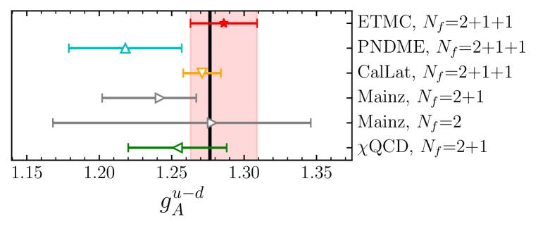
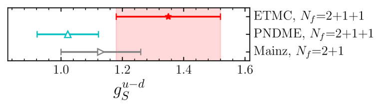
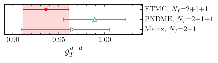
In Fig. 14 we compare with recent results from other lattice collaborations considering only results computed using simulations with approximately physical pion mass i.e. excluding chiral extrapolations. This provides a fair comparison among the lattice QCD results. In Fig. 15 we compare our results with recent lattice QCD results obtained after performing chiral and continuum extrapolation. They include at least one ensemble with mass about 200 MeV or lower. The final results by the PNDME Gupta et al. (2018a) and CalLat Chang et al. (2018) collaborations shown in Fig. 15 are obtained by combining measurements from several ensembles with different lattice spacing, volume and pion mass. They include two measurements at the physical pion mass that are also included in Fig. 14 as well as the final value after a combined chiral and continuum extrapolation. CalLat quotes as their final value and PNDME . As can be seen, the final values by both PNDME and CalLat are in agreement with their results using the physical point ensembles, but with a much smaller error for the latter. The CalLat value is in perfect agreement with our value. Furthermore, the lattice results computed for a given ensemble over a range of lattice spacings shown in Fig. 14 are in good agreement demonstrating that lattice spacing effects are indeed small.
For the case of , we find a value that is larger as compared to other lattice QCD determinations, which can be explained by the fact that increases with . In our analysis of the cB211.072.64 ensemble seven values of are used reaching larger time separations combined with increased statistics that allow for a better control of excited states von Hippel et al. (2017), as demonstrated in the Appendix. Similarly, our value for tends to be smaller since this quantity decreases with increasing values of . As we already stressed, given that the analysis for the cB211.072.64 ensemble is the most thorough having the largest statistics and the biggest number of , we consider as final the values extracted using this ensemble. In Fig. 15 we include the values of and obtained by the PNDME and CLS collaborations after chiral and continuum extrapolation. The chirally extrapolated values by PNDME are consistent with their value using the two physical ensembles, corroborating the fact that finite discretization effects are small and consistent with our findings using heavier than physical pion mass Alexandrou et al. (2011). The computation by the CLS Mainz group used ensembles with a smallest pion mass of about 200 MeV and it is in agreement with our values.
| 1.286(23) | 0.530(18) | 0.422(25) | 0.382(31) | |
| 1.35(17) | 9.92(90) | 11.1(1.0) | 11.4(1.0) | |
| 0.936(25) | 0.527(22) | 0.519(22) | 0.518(22) | |
| 0.862(17) | -0.424(16) | -0.0458(73) | -0.0098(34) | |
| 6.09(55) | 4.74(43) | 0.454(61) | 0.075(17) | |
| 0.729(22) | -0.2075(75) | -0.00268(58) | -0.00024(16) |
The values extracted for the renormalized isovector, isoscalar and single flavor charges are tabulated in Tables 10 and 11 for the cA2.09.48 and cB211.072.64 ensembles respectively. The latter are our best determination of these quantities and in particular the precision obtained in the determination of the single flavor charges computed directly at the physical point using this ensemble is much better as compared to any other available lattice QCD results. This includes also our previous determination Alexandrou et al. (2017b, a) using the cA2.09.48 ensemble. In particular, we find for the first time, for , and a non-zero value showing charm quark effects.
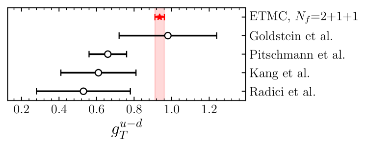
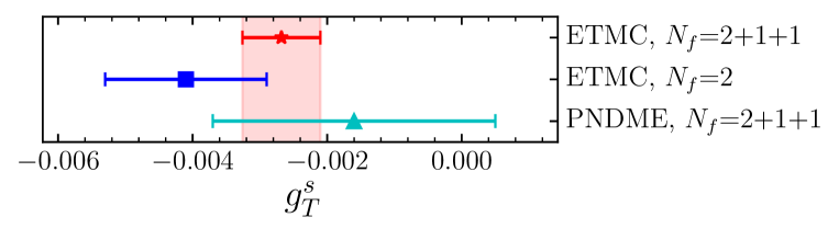
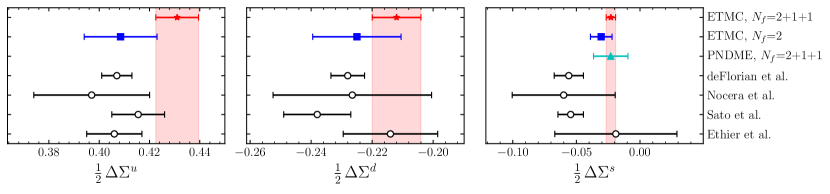
In Figs. 16 and 17 we show a comparison of available lattice QCD results for the tensor charges and intrinsic spin contributions of quarks, , to the proton computed directly at the physical point111The results of the PNDME collaboration for the connected contributions and for the strange charges are of comparable quality Gupta et al. (2018a); Lin et al. (2018b). We note that the result of PNDME after chiral and continuum extrapolation is consistent with their value using the physical ensemble. However, the disconnected contributions to the up and down quarks have not been computed at the physical point and thus we do not include them in Fig. 17. One can find the values without the disconnected contributions in Ref. Lin et al. (2018b).. We also include phenomenological results, where we limit ourselves to those that have not used input from lattice QCD. A good agreement is observed among lattice QCD results and a notable observation is that the lattice QCD results are at least as accurate as the phenomenological determinations.
PCAC relates to the pseudoscalar charge through the relation González-Alonso and Martin Camalich (2014). Using our values for , the relation
| (13) |
where is the twisted mass parameter in lattice units used in the simulation of the cB211.072.64 ensemble, and the extracted value of the nucleon mass we obtain . This value is lower as compared to found in Ref. González-Alonso and Martin Camalich (2014). A direct evaluation of in lattice QCD using the same setup will be undertaken in the future to study the origin of this discrepancy.
V.2 Nucleon -terms
| [MeV] | 41.6(3.8) | 45.6(6.2) | 107(22) |
|---|---|---|---|
| 0.0444(43) | 0.0487(68) | 0.115(24) |
The nucleon -terms that give the scalar quark contents are fundamental quantities of QCD. They determine the mass generated by the quarks in the nucleon. They are relevant for a wide range of physical processes and for the interpretation of direct-detection dark matter (DM) searches Giedt et al. (2009) being undertaken by a number of experiments Cushman et al. (2013). It is customary to define the nucleon -terms to be scheme- and scale-independent quantities:
| (14) |
for a given quark of flavor , or for the isoscalar combination, where is the mass of , is the average light quark mass and is the nucleon state.
Since the pioneering chiral perturbation theory analysis that yielded MeV Gasser et al. (1991), there has been significant progress in the determination of from experimental data Hoferichter et al. (2012); Alarcon et al. (2012). Using high-precision data from pionic atoms to determine the -scattering lengths and a system of Roy-Steiner equations that encode constraints from analyticity, unitarity, and crossing symmetry a value of MeV is obtained Hoferichter et al. (2015). This larger value of has theoretical implications on our understanding of the strong interactions as stressed in Ref. Leutwyler (2015). Given the importance of these quantities, a number of lattice QCD calculations have been undertaken to compute them using two approaches Young and Thomas (2010). The first uses the Feynman-Hellmann theorem that is based on the variation of the nucleon mass with : . However, since the dependence of the nucleon mass on the strange and charm quark mass is weak, this approach yields large errors. An alternative method is to evaluate directly the nucleon matrix elements of the scalar operator that involves disconnected quark loops as done in this work. The evaluation of the three-point function is computationally much more demanding than hadron masses. Therefore, it is only recently that a direct computation of the -terms has been performed using dynamical simulations Bali et al. (2012); Freeman and Toussaint (2013); Gong et al. (2013); Abdel-Rehim et al. (2014); Alexandrou et al. (2015); Yang et al. (2016); Bali et al. (2016).
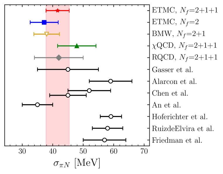
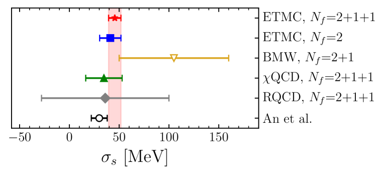
The values extracted for the -terms and are tabulated in Table 12 for the cB211.072.64 ensemble. We show results for the - and -terms in Fig. 18 computed by various lattice QCD collaborations at the physical point either directly by computing the three-point function or using the Feynman-Hellmann method that include ensembles at the physical point. We also compare with phenomenological results limiting ourselves to those that have not used input from lattice QCD. We observe a very good agreement among lattice QCD results. One can see the very large uncertainty on by BMW when extracted using the Feynman-Hellmann method.
It is customary to also provide results in terms of the dimensionless ratios, . Since we have the isovector matrix element , for the cB211.072.64 ensemble, we can combine it with the isoscalar matrix element to obtain the individual up- and down-quark contributions for the proton and the neutron in the isospin limit via the relations
| (15) |
where the up and down quark mass splitting entering in and is computed taking the ratio of the up to the down quark masses from Ref. Aoki et al. (2019) together with our determination of the up and down quark mass, as given in Eq. (13). We obtain
| (16) |
These results are compatible with the results of our previous study using the cA2.09.48 ensemble Abdel-Rehim et al. (2016). The isovector scalar charge is also related to the neutron-proton mass splitting in the absence of electromagnetism González-Alonso and Martin Camalich (2014) through the relation . We thus obtain
| (17) |
and we find MeV. This value is consistent with MeV determined for non-degenerate up- and down-quarks Borsanyi et al. (2015).
The y-parameter, defined as , gives a measure of the strangeness content of the nucleon. We find a value of for the cB211.072.64 ensemble.
VI Conclusions
Results on the nucleon axial, tensor and scalar charges are presented for three ensembles of twisted mass clover-improved fermions tuned to reproduce the physical value of the pion mass. The most thorough analysis is performed for the ensemble which provides one of the best descriptions of the QCD vacuum to date having light, strange and charm quarks in the sea. A notable result of this work is the accurate computation of using the cB211.072.64 ensemble that agrees with the experimental value of 1.27641(56) Märkisch et al. (2019). An additional milestone is the evaluation to an unprecedented accuracy of the flavor charges directly at the physical point taking into account the disconnected contributions. We show that the charm axial charge is non-zero and obtain a value for that is more accurate than recent phenomenological determinations. It confirms the smaller values recently suggested by the NNPDF Nocera et al. (2014) and JAM17 Ethier et al. (2017) analyses both of which, however, carry a large error. We find that the intrinsic quark spin contribution in the nucleon is . The non-singlet combination is found to be . Furthermore, the evaluation of the isovector scalar and tensor charges to an accuracy of about 10% and 3%, respectively provides valuable input to experimental studies on possible allowed scalar and tensor interactions and new physics searches Bhattacharya et al. (2012).
Using the scalar matrix element we extract the nucleon -terms that are important for direct dark matter searches and for phenomenological studies of scattering processes. We find MeV, that confirms a smaller value already suggested from previous lattice QCD studies Abdel-Rehim et al. (2016); Yang et al. (2016); Bali et al. (2012). While this smaller value is in agreement with the first analysis that yielded MeV Gasser et al. (1991), it is in tension with recent analyses that yield larger values. An analysis based on the Roy-Steiner equations and experimental data on pionic atoms extracted the value of MeV Hoferichter et al. (2015) that is confirmed by using a large-scale fit of pionic-atom level shift and width data across the periodic table Friedman and Gal (2019). The larger value is also confirmed by using the scattering lengths from the low-energy data base Ruiz de Elvira et al. (2018). Given the significant progress in the determination of both using experimental data Hoferichter et al. (2016, 2012); Alarcon et al. (2012) and lattice QCD this persisting tension needs to be further examined. Computing the scattering lengths within lattice QCD will provide a crucial cross-check.
ACKNOWLEDGMENTS
We acknowledge funding from the European Union’s Horizon 2020 research and innovation programme under the Marie Sklodowska-Curie grant agreement No 642069 and from the COMPLEMENTARY/0916/0015 project funded by the Cyprus Research Promotion Foundation. M.C. acknowledges financial support by the U.S. National Science Foundation under Grant No. PHY-1714407. This work was supported by a grant from the Swiss National Supercomputing Centre (CSCS) under project ID s702. We thank the staff of CSCS for access to the computational resources and for their constant support. The Gauss Centre for Supercomputing e.V. (www.gauss-centre.eu) funded the project pr74yo by providing computing time on the GCS Supercomputer SuperMUC at Leibniz Supercomputing Centre (www.lrz.de). In addition, this work used computational resources from Extreme Science and Engineering Discovery Environment (XSEDE), which is supported by National Science Foundation grant number TG-PHY170022. This work used computational resources from the John von Neumann-Institute for Computing on the JUWELS system at the research center in Jülich, under the project with id ECY00 and HCH02. K.H. is financially supported by the Cyprus Research Promotion foundation under contract number POST-DOC/0718/0100.
APPENDIX
We examine here in more detail the importance of increasing the statistics in the three-point functions as we increase the source-sink time separation in order to keep the statistical error approximately constant. This is carried out for the cB211.072.64 ensemble for which we increase the statistics as listed in Table 2 at each . As we will show below, excited state effects are only correctly addressed if the statistics are sufficiently large to keep the errors approximately the same among the various values of .
VI.1 Plateau method
We first examine the plateau method for the case of the isovector charge operators. We show in the left panel of Fig. 19 the plateau values that one would obtain if one kept the statistics the same as at the smallest value for all the source-sink time separations instead of the ones given in Table 2. As can be seen the errors increase becoming very large for the two largest time separations. With such errors one might think that convergence is reached already at fm, shown by the open red symbol. For for which effects of excited state are milder one would obtain a value compatible with the one extracted from the two-state fit. However, a weighted average would yield a lower value for and a larger one for , as shown by the gray bands. This is to be contrasted with the values extracted using the increased statistics of Table 2 for larger values, shown in the right panel of Fig. 19. For both and there is a clear indication that excited states are still present and even larger time separations are needed to be sure that one has converged to the two-state result depicted by the red band.
VI.2 Two-state fit method
Our data show also that the two-state fit approach cannot capture correctly excited state effects if the error increases with the source-sink separation. This is specially seen for the tensor charge as depicted in Fig. 20 we show results extracted using the two-state fit approach considering five different cases:
-
•
Using the three smaller values of keeping the statistics the same as that of the smallest , namely 750. Since the smallest is the most accurate its weight in the fit is large and the error band increases as increases, resulting in a mean value for and that is below the one obtained if one uses the full statistics shown by the red band. Given the large error in particular for the two results are consistent. However, for the fit yields a value that clearly overestimates the value extracted when using the full statistics.
-
•
Using all values of but keeping the statistics at 750 for all. A similar behavior is observed despite the fact that we now have seven time separations instead of three since the fits are dominated by the smallest and most accurate point. Therefore, having results at larger time separations, without increasing statistics is not very useful.
-
•
Using fm, 1.12 fm and 1.28 fm keeping the statistics at 3000, namely the same as for the smallest used in the fit. Having larger time separations with more statistics tends to increase the mean values of and , but once more the fit is heavily biased b the first most accurate point, resulting in a larger value for .
-
•
Using all values greater than fm but keeping the statistics the same as for fm. Similar results are obtained as with the previous case.
- •
As this study shows it is important to both have sink-source time separations that span a large enough range and also to increase statistics so the errors at each time separation are approximately constant. Otherwise, the two-state fit is driven by the most accurate point and can lead to wrong results.
References
- Mendenhall et al. (2013) M. P. Mendenhall et al. (UCNA), Phys. Rev. C87, 032501 (2013), eprint 1210.7048.
- Mund et al. (2013) D. Mund, B. Maerkisch, M. Deissenroth, J. Krempel, M. Schumann, H. Abele, A. Petoukhov, and T. Soldner, Phys. Rev. Lett. 110, 172502 (2013), eprint 1204.0013.
- Märkisch et al. (2019) B. Märkisch et al., Phys. Rev. Lett. 122, 242501 (2019), eprint 1812.04666.
- Bhattacharya et al. (2012) T. Bhattacharya, V. Cirigliano, S. D. Cohen, A. Filipuzzi, M. Gonzalez-Alonso, M. L. Graesser, R. Gupta, and H.-W. Lin, Phys. Rev. D85, 054512 (2012), eprint 1110.6448.
- Bischer and Rodejohann (2019) I. Bischer and W. Rodejohann, Phys. Rev. D 99, 036006 (2019), URL https://link.aps.org/doi/10.1103/PhysRevD.99.036006.
- Akimov et al. (2017) D. Akimov et al., Science 357, 1123 (2017), ISSN 0036-8075, eprint https://science.sciencemag.org/content/357/6356/1123.full.pdf, URL https://science.sciencemag.org/content/357/6356/1123.
- Abs et al. (2015) M. Abs et al. (2015), eprint 1511.05130.
- Akerib et al. (2015) D. Akerib et al. (LZ) (2015), eprint 1509.02910.
- Beda et al. (2012) A. Beda, V. Brudanin, V. Egorov, D. Medvedev, V. Pogosov, M. Shirchenko, and A. Starostin, Adv. High Energy Phys. 2012, 350150 (2012).
- Wong et al. (2007) H. T. Wong, H. B. Li, S. T. Lin, F. S. Lee, V. Singh, S. C. Wu, C. Y. Chang, H. M. Chang, C. P. Chen, M. H. Chou, et al. (TEXONO Collaboration), Phys. Rev. D 75, 012001 (2007), URL https://link.aps.org/doi/10.1103/PhysRevD.75.012001.
- Yamanaka, N. et al. (2017) Yamanaka, N., Sahoo, B. K., Yoshinaga, N., Sato, T., Asahi, K., and Das, B. P., Eur. Phys. J. A 53, 54 (2017), URL https://doi.org/10.1140/epja/i2017-12237-2.
- Delaunay et al. (2017) C. Delaunay, C. Frugiuele, E. Fuchs, and Y. Soreq, Phys. Rev. D 96, 115002 (2017), URL https://link.aps.org/doi/10.1103/PhysRevD.96.115002.
- Marrodán Undagoitia and Rauch (2016) T. Marrodán Undagoitia and L. Rauch, J. Phys. G 43, 013001 (2016), eprint 1509.08767.
- Chizhov (1996) M. Chizhov, Physics Letters B 381, 359 (1996), ISSN 0370-2693, URL http://www.sciencedirect.com/science/article/pii/0370269396005357.
- Dhargyal (2018) L. Dhargyal, Springer Proc. Phys. 203, 329 (2018), eprint 1610.06293.
- Adolph et al. (2014) C. Adolph et al. (COMPASS), Phys. Lett. B736, 124 (2014), eprint 1401.7873.
- Ye et al. (2017) Z. Ye, N. Sato, K. Allada, T. Liu, J.-P. Chen, H. Gao, Z.-B. Kang, A. Prokudin, P. Sun, and F. Yuan, Phys. Lett. B767, 91 (2017), eprint 1609.02449.
- Bhattacharya et al. (2016) T. Bhattacharya, V. Cirigliano, S. Cohen, R. Gupta, H.-W. Lin, and B. Yoon, Phys. Rev. D94, 054508 (2016), eprint 1606.07049.
- Glashow and Weinberg (1968) S. Glashow and S. Weinberg, Physical Review Letters 20, 224 (1968).
- González-Alonso and Martin Camalich (2014) M. González-Alonso and J. Martin Camalich, Phys. Rev. Lett. 112, 042501 (2014), eprint 1309.4434.
- Gasser and Leutwyler (1982) J. Gasser and H. Leutwyler, Phys. Rept. 87, 77 (1982).
- Crewther et al. (1979) R. Crewther, P. Di Vecchia, G. Veneziano, and E. Witten, Phys. Lett. B 88, 123 (1979), [Erratum: Phys.Lett.B 91, 487 (1980)].
- Lin et al. (2018a) H.-W. Lin et al., Prog. Part. Nucl. Phys. 100, 107 (2018a), eprint 1711.07916.
- Chang et al. (2018) C. C. Chang et al., Nature 558, 91 (2018), eprint 1805.12130.
- Aoki et al. (2019) S. Aoki et al. (Flavour Lattice Averaging Group) (2019), eprint 1902.08191.
- Abdel-Rehim et al. (2017) A. Abdel-Rehim et al. (ETM), Phys. Rev. D95, 094515 (2017), eprint 1507.05068.
- Alexandrou et al. (2018a) C. Alexandrou et al., Phys. Rev. D98, 054518 (2018a), eprint 1807.00495.
- Frezzotti et al. (2001) R. Frezzotti, P. A. Grassi, S. Sint, and P. Weisz (Alpha), JHEP 08, 058 (2001), eprint hep-lat/0101001.
- Frezzotti and Rossi (2004) R. Frezzotti and G. C. Rossi, JHEP 08, 007 (2004), eprint hep-lat/0306014.
- Sheikholeslami and Wohlert (1985) B. Sheikholeslami and R. Wohlert, Nucl. Phys. B259, 572 (1985).
- Alexandrou et al. (2011) C. Alexandrou, M. Brinet, J. Carbonell, M. Constantinou, P. A. Harraud, P. Guichon, K. Jansen, T. Korzec, and M. Papinutto (ETM), Phys. Rev. D83, 045010 (2011), eprint 1012.0857.
- Frezzotti et al. (2006) R. Frezzotti, G. Martinelli, M. Papinutto, and G. C. Rossi, JHEP 04, 038 (2006), eprint hep-lat/0503034.
- Boucaud et al. (2008) P. Boucaud et al. (ETM), Comput. Phys. Commun. 179, 695 (2008), eprint 0803.0224.
- Osterwalder and Seiler (1978) K. Osterwalder and E. Seiler, Annals Phys. 110, 440 (1978).
- Alexandrou and Kallidonis (2017) C. Alexandrou and C. Kallidonis, Phys. Rev. D96, 034511 (2017), eprint 1704.02647.
- Alexandrou et al. (2017a) C. Alexandrou, M. Constantinou, K. Hadjiyiannakou, K. Jansen, C. Kallidonis, G. Koutsou, and A. Vaquero Aviles-Casco, Phys. Rev. D96, 054507 (2017a), eprint 1705.03399.
- Alexandrou et al. (2017b) C. Alexandrou et al., Phys. Rev. D95, 114514 (2017b), [Erratum: Phys. Rev.D96,no.9,099906(2017)], eprint 1703.08788.
- Alexandrou et al. (2017c) C. Alexandrou, M. Constantinou, K. Hadjiyiannakou, K. Jansen, C. Kallidonis, G. Koutsou, A. Vaquero Avilés-Casco, and C. Wiese, Phys. Rev. Lett. 119, 142002 (2017c), eprint 1706.02973.
- Alexandrou et al. (1994) C. Alexandrou, S. Gusken, F. Jegerlehner, K. Schilling, and R. Sommer, Nucl. Phys. B414, 815 (1994), eprint hep-lat/9211042.
- Gusken (1990) S. Gusken, Nucl. Phys. Proc. Suppl. 17, 361 (1990).
- Albanese et al. (1987) M. Albanese et al. (APE), Phys. Lett. B192, 163 (1987).
- Frommer et al. (2014) A. Frommer, K. Kahl, S. Krieg, B. Leder, and M. Rottmann, SIAM J. Sci. Comput. 36, A1581 (2014), eprint 1303.1377.
- Alexandrou et al. (2016) C. Alexandrou, S. Bacchio, J. Finkenrath, A. Frommer, K. Kahl, and M. Rottmann, Phys. Rev. D94, 114509 (2016), eprint 1610.02370.
- Alexandrou et al. (2018b) C. Alexandrou, S. Bacchio, M. Constantinou, J. Finkenrath, K. Hadjiyiannakou, K. Jansen, G. Koutsou, and A. V. A. Casco (2018b), eprint 1812.10311.
- Stathopoulos et al. (2013) A. Stathopoulos, J. Laeuchli, and K. Orginos (2013), eprint 1302.4018.
- Michael and Urbach (2007) C. Michael and C. Urbach (ETM), PoS LATTICE2007, 122 (2007), eprint 0709.4564.
- McNeile and Michael (2006) C. McNeile and C. Michael (UKQCD), Phys. Rev. D73, 074506 (2006), eprint hep-lat/0603007.
- von Hippel et al. (2017) G. von Hippel, T. D. Rae, E. Shintani, and H. Wittig, Nucl. Phys. B914, 138 (2017), eprint 1605.00564.
- Bar (2019) O. Bar, Phys. Rev. D 99, 054506 (2019), eprint 1812.09191.
- Capitani et al. (2012) S. Capitani, M. Della Morte, G. von Hippel, B. Jager, A. Juttner, B. Knippschild, H. B. Meyer, and H. Wittig, Phys. Rev. D86, 074502 (2012), eprint 1205.0180.
- Abdel-Rehim et al. (2014) A. Abdel-Rehim, C. Alexandrou, M. Constantinou, V. Drach, K. Hadjiyiannakou, K. Jansen, G. Koutsou, and A. Vaquero, Phys. Rev. D89, 034501 (2014), eprint 1310.6339.
- Martinelli et al. (1995) G. Martinelli, C. Pittori, C. T. Sachrajda, M. Testa, and A. Vladikas, Nucl. Phys. B445, 81 (1995), eprint hep-lat/9411010.
- Gockeler et al. (1999) M. Gockeler, R. Horsley, H. Oelrich, H. Perlt, D. Petters, P. E. Rakow, A. Schafer, G. Schierholz, and A. Schiller, Nucl. Phys. B 544, 699 (1999), eprint hep-lat/9807044.
- Alexandrou et al. (2012) C. Alexandrou, M. Constantinou, T. Korzec, H. Panagopoulos, and F. Stylianou, Phys. Rev. D86, 014505 (2012), eprint 1201.5025.
- Constantinou et al. (2009) M. Constantinou, V. Lubicz, H. Panagopoulos, and F. Stylianou, JHEP 10, 064 (2009), eprint 0907.0381.
- Alexandrou et al. (2017d) C. Alexandrou, M. Constantinou, and H. Panagopoulos (ETM), Phys. Rev. D95, 034505 (2017d), eprint 1509.00213.
- Skouroupathis and Panagopoulos (2009) A. Skouroupathis and H. Panagopoulos, Phys. Rev. D79, 094508 (2009), eprint 0811.4264.
- Hasan et al. (2019) N. Hasan, J. Green, S. Meinel, M. Engelhardt, S. Krieg, J. Negele, A. Pochinsky, and S. Syritsyn, Phys. Rev. D99, 114505 (2019), eprint 1903.06487.
- Shintani et al. (2019) E. Shintani, K.-I. Ishikawa, Y. Kuramashi, S. Sasaki, and T. Yamazaki, Phys. Rev. D99, 014510 (2019), eprint 1811.07292.
- Gupta et al. (2018a) R. Gupta, Y.-C. Jang, B. Yoon, H.-W. Lin, V. Cirigliano, and T. Bhattacharya, Phys. Rev. D98, 034503 (2018a), eprint 1806.09006.
- Harris et al. (2019) T. Harris, G. von Hippel, P. Junnarkar, H. B. Meyer, K. Ottnad, J. Wilhelm, H. Wittig, and L. Wrang, Phys. Rev. D 100, 034513 (2019), eprint 1905.01291.
- Capitani et al. (2019) S. Capitani, M. Della Morte, D. Djukanovic, G. M. von Hippel, J. Hua, B. Jäger, P. M. Junnarkar, H. B. Meyer, T. D. Rae, and H. Wittig, Int. J. Mod. Phys. A 34, 1950009 (2019), eprint 1705.06186.
- Liang et al. (2018) J. Liang, Y.-B. Yang, T. Draper, M. Gong, and K.-F. Liu, Phys. Rev. D 98, 074505 (2018), eprint 1806.08366.
- Lin et al. (2018b) H.-W. Lin, R. Gupta, B. Yoon, Y.-C. Jang, and T. Bhattacharya, Phys. Rev. D98, 094512 (2018b), eprint 1806.10604.
- Gupta et al. (2018b) R. Gupta, B. Yoon, T. Bhattacharya, V. Cirigliano, Y.-C. Jang, and H.-W. Lin, Phys. Rev. D98, 091501 (2018b), eprint 1808.07597.
- Goldstein et al. (2014) G. R. Goldstein, J. O. Gonzalez Hernandez, and S. Liuti (2014), eprint 1401.0438.
- Pitschmann et al. (2015) M. Pitschmann, C.-Y. Seng, C. D. Roberts, and S. M. Schmidt, Phys. Rev. D91, 074004 (2015), eprint 1411.2052.
- Kang et al. (2016) Z.-B. Kang, A. Prokudin, P. Sun, and F. Yuan, Phys. Rev. D93, 014009 (2016), eprint 1505.05589.
- Radici and Bacchetta (2018) M. Radici and A. Bacchetta, Phys. Rev. Lett. 120, 192001 (2018), eprint 1802.05212.
- de Florian et al. (2009) D. de Florian, R. Sassot, M. Stratmann, and W. Vogelsang, Phys. Rev. D80, 034030 (2009), eprint 0904.3821.
- Nocera et al. (2014) E. R. Nocera, R. D. Ball, S. Forte, G. Ridolfi, and J. Rojo (NNPDF), Nucl. Phys. B887, 276 (2014), eprint 1406.5539.
- Sato et al. (2016) N. Sato, W. Melnitchouk, S. E. Kuhn, J. J. Ethier, and A. Accardi (Jefferson Lab Angular Momentum), Phys. Rev. D93, 074005 (2016), eprint 1601.07782.
- Ethier et al. (2017) J. J. Ethier, N. Sato, and W. Melnitchouk, Phys. Rev. Lett. 119, 132001 (2017), eprint 1705.05889.
- Abdel-Rehim et al. (2016) A. Abdel-Rehim, C. Alexandrou, M. Constantinou, K. Hadjiyiannakou, K. Jansen, C. Kallidonis, G. Koutsou, and A. Vaquero Aviles-Casco (ETM), Phys. Rev. Lett. 116, 252001 (2016), eprint 1601.01624.
- Yang et al. (2016) Y.-B. Yang, A. Alexandru, T. Draper, J. Liang, and K.-F. Liu (xQCD), Phys. Rev. D94, 054503 (2016), eprint 1511.09089.
- Bali et al. (2016) G. S. Bali, S. Collins, D. Richtmann, A. Schäfer, W. Söldner, and A. Sternbeck (RQCD), Phys. Rev. D93, 094504 (2016), eprint 1603.00827.
- Durr et al. (2016) S. Durr et al., Phys. Rev. Lett. 116, 172001 (2016), eprint 1510.08013.
- Gasser et al. (1991) J. Gasser, H. Leutwyler, and M. E. Sainio, Phys. Lett. B253, 252 (1991).
- Alarcon et al. (2012) J. M. Alarcon, J. Martin Camalich, and J. A. Oller, Phys. Rev. D85, 051503 (2012), eprint 1110.3797.
- Chen et al. (2013) Y.-H. Chen, D.-L. Yao, and H. Q. Zheng, Phys. Rev. D87, 054019 (2013), eprint 1212.1893.
- An and Saghai (2015) C. S. An and B. Saghai, Phys. Rev. D92, 014002 (2015), eprint 1404.2389.
- Hoferichter et al. (2015) M. Hoferichter, J. Ruiz de Elvira, B. Kubis, and U.-G. Meißner, Phys. Rev. Lett. 115, 092301 (2015), eprint 1506.04142.
- Ruiz de Elvira et al. (2018) J. Ruiz de Elvira, M. Hoferichter, B. Kubis, and U.-G. Meissner, J. Phys. G45, 024001 (2018), eprint 1706.01465.
- Friedman and Gal (2019) E. Friedman and A. Gal, Phys. Lett. B792, 340 (2019), eprint 1901.03130.
- Giedt et al. (2009) J. Giedt, A. W. Thomas, and R. D. Young, Phys. Rev. Lett. 103, 201802 (2009), eprint 0907.4177.
- Cushman et al. (2013) P. Cushman et al., in Proceedings, 2013 Community Summer Study on the Future of U.S. Particle Physics: Snowmass on the Mississippi (CSS2013): Minneapolis, MN, USA, July 29-August 6, 2013 (2013), eprint 1310.8327, URL http://www.slac.stanford.edu/econf/C1307292/docs/CosmicFrontier/WIMPDirect-24.pdf.
- Hoferichter et al. (2012) M. Hoferichter, C. Ditsche, B. Kubis, and U. G. Meissner, JHEP 06, 063 (2012), eprint 1204.6251.
- Leutwyler (2015) H. Leutwyler, PoS CD15, 022 (2015), eprint 1510.07511.
- Young and Thomas (2010) R. D. Young and A. W. Thomas, Nucl. Phys. A844, 266C (2010), eprint 0911.1757.
- Bali et al. (2012) G. S. Bali et al. (QCDSF), Phys. Rev. D85, 054502 (2012), eprint 1111.1600.
- Freeman and Toussaint (2013) W. Freeman and D. Toussaint (MILC), Phys. Rev. D88, 054503 (2013), eprint 1204.3866.
- Gong et al. (2013) M. Gong et al. (XQCD), Phys. Rev. D88, 014503 (2013), eprint 1304.1194.
- Alexandrou et al. (2015) C. Alexandrou, M. Constantinou, S. Dinter, V. Drach, K. Hadjiyiannakou, K. Jansen, G. Koutsou, and A. Vaquero, Phys. Rev. D91, 094503 (2015), eprint 1309.7768.
- Borsanyi et al. (2015) S. Borsanyi et al., Science 347, 1452 (2015), eprint 1406.4088.
- Hoferichter et al. (2016) M. Hoferichter, J. Ruiz de Elvira, B. Kubis, and U.-G. Meissner, Phys. Rept. 625, 1 (2016), eprint 1510.06039.