Equitable colorings of hypergraphs with few edges

Abstract

The paper deals with an extremal problem concerning equitable colorings of uniform hypergraph. Recall that a vertex coloring of a hypergraph $H$ is called proper if there are no monochro-matic edges under this coloring. A hypergraph is said to be equitably $r$-colorable if there is a proper coloring with $r$ colors such that the sizes of any two color classes differ by at most one. In the present paper we prove that if the number of edges $|E(H)|\leq 0.01\left(\frac{n}{\ln n}\right)^{\frac{r-1}{r}}r^{n-1}$ then the hypergraph $H$ is equitably $r$-colorable provided $r<\sqrt[5]{\ln n}$.

Keywords: uniform hypergraphs, proper colorings, equitable colorings, Pluhár’s criterion.

1 Introduction

The present paper deals with the well-known problem concerning colorings of hypergraphs. Let us start with recalling some definitions.

1.1 Main definitions and new result

Let $H=(V,E)$ be a hypergraph. A coloring of the vertex set $V$ of a hypergraph $H=(V,E)$ is called proper if none of the edges in $E$ is monochromatic under this coloring. A hypergraph is said to be $r$-colorable if there exists a proper coloring with $r$ colors for it. A coloring of the hypergraph vertices is said to be equitable if it is proper and the sizes of any two of color classes differ by at most one. The last means that the set of vertices $V$ can be divided not just into $r$ independent sets, but into $r$ independent sets of almost the same size.

The main result of the paper provides a sufficient condition for admitting an equitable $r$-coloring by an $n$-uniform hypergraph as the restriction on the number of edges.

Theorem 1.

For large enough $n$, if $r<\sqrt[5]{\ln n}$ then any $n$-uniform hypergraph $H=(V,E)$ with

$$|E|\leq 0.01\left(\frac{n}{\ln n}\right)^{\frac{r-1}{r}}r^{n-1}$$

is equitably $r$-colorable provided $|V|$ is divisible by $r$.

1.2 Related work and method

Let us begin with well-known extremal problem concerning hypergraphs colorings. This whole thing started when Erdős and Hajnal proposed to find the value $m(n,r)$ which is equal to the smallest number of edges in an $n$-uniform none-$r$-colorable hypergraph. We will only note that for small $r$ in comparison with $n$, the best current bounds are the following:

$$c_{1}\left(\frac{n}{\ln n}\right)^{\frac{r-1}{r}}r^{n-1}\leq m(n,r)\leq c_{2}n^{2}r^{n}\ln r,$$ (1)

were $c_{1},c_{2}>0$ are some absolute constants. The lower bound was proved by Kozik and Cherkashin[1], the proof of upper bound is that of Erdős (see the proof in Kostochka’s paper [2]). In fact, the result of Kozik and Cherkashin remains true for large $r$ compared to $n$, but in this case, Akolzin and Shabanov proved more stronger estimates [3]. Reader can find more results on the related problems in [4]–[7]. Recent advances concerning colorings of random hypergraphs were obtained in [8]–[11].

Now we will move on to history of equitable colorings. A significant interest in equitable colorings historically arose in connection with the celebrated theorem of Hajnal and Szemerédi [12] of 1970, which verified the following conjecture of Erdős [13]: every graph $G$ with maximal vertex degree $\Delta(G)$ admits not only a proper but also an equitable coloring with $\Delta+1$ colors.

It is worth noting that the original proof of Hajnal and Szemerédi [12] was long enough and complicated. In 2008 Kierstead and Kostochka [14] presented another proof, that was short and transparent. Moreover, they refined this result to the case of maximum edge degree [15] and together with Mydlarz and Szemerédi found a fast algorithm for obtaining an equitable coloring [16].

The generalization of Erdős’s conjecture to uniform hypergraphs was obtained by Lu and Székely. Namely, they proved that: if $|V|$ is divisible by $r$ and the maximum vertex degree $\Delta(H)\leq\ r^{n-1}/(2en),$ then $H$ admits an equitable $r$-coloring [17].

The main aim of the present paper is to give the sufficient condition for an equitable $r$-colorability of a hypergraph as a restriction on the number of edges in the general class of $n$-uniform hypergraphs. In other words, we study the analog of the Erdős–Hajnal problem for equitable colorings [18]. We also stress, that the previous best known bound that guarantees the existence of an equitable $r$-coloring of an $n$-uniform hypergraph was just $r^{n-1}$.

The proof of Theorem 1 is based on the idea that there is a coloring in which there are few specific configurations, so-called ordered $k$-chains, where $k\in\{1,2,...,r\}$. The idea of considering ordered $r$-chains was first conceived and proved by Pluha̋r [19]: an arbitrary hypergraph is $r$-colorable if and only if there exists order on $V$ without ordered $r$-chains. The similar idea was used by Cherkashin and Kozik [1], who get the best known result for the case when $n$ is big enough in comparison with $r$.

Let’s get back to Theorem 1. The crucial moment is that: Pluha̋r criterion does not provide the information on the cardinalities of color classes, while consideration of ordered chains of all sizes does provide it.

The rest of the paper is organized as follows. In Section 2 we show that the theorem holds for hypergraphs with few vertices. Section 3 is devoted to the random algorithm, which with positive probability creates proper, but not necessarily equitable $r$-coloring of $H$. In Section 4, by the recoloring of few vertices, we will ensure the equalities of sizes of the color classes keeping the lack of the monochromatic edges.

2 Hypergraphs with few vertices

Assume that $H=(V,E)$ is a hypergraph from Theorem 1. Let $m=|V|$ denote its number of vertices. The aim of this paragraph is to show that the following conditions:

$$|E|<0.01\left(\frac{n}{\ln n}\right)^{\frac{r-1}{r}}r^{n-1},\leavevmode\nobreak\ \leavevmode\nobreak\ \leavevmode\nobreak\ |V|<\frac{n^{2}(r-1)}{2\ln n},$$ (2)

imply that the hypergraph $H$ admits an equitable coloring with $r$ colors. For this purpose, it is sufficient to consider a random balanced coloring with $r$ colors. A coloring is said to be balanced if the sizes of its color classes are equal, i.e. it is a partition of $V$ into $r$ parts with the same size: $V=K_{1}\sqcup K_{1}...\sqcup K_{r-1},|K_{1}|=|K_{2}|=...=|K_{r}|=m/r$.

Let $C$ be a random balanced coloring of $V$ with $r$ colors. Then for any edge $A\in E$,

$$\mathop{\kern 0.0pt\mathsf{P}}\nolimits(\text{$A$ is monochromatic under $C$})=\frac{r\binom{m-n}{m/r-n}}{\binom{m}{m/r}}.$$

Thus,

$$\mathop{\kern 0.0pt\mathsf{P}}\nolimits( \text{there exists a monochromatic edge under $C$})\leq$$

$$=|E|\frac{r\binom{m-n}{m/r-n}}{\binom{m}{m/r}}=|E|\frac{r^{-n+1}(1-r/m)...(1-r(n-1)/m)}{(1-1/m)...(1-(n-1)/m)}\leq$$

$$\leq 0.01\left(\frac{n}{\ln n}\right)^{\frac{r-1}{r}}\frac{\exp(\ln(1-r/m)+...+\ln(1-r(n-1)/m))}{\exp(\ln(1-1/m)+...+\ln(1-(n-1)/m))}=$$

$$=0.01\left(\frac{n}{\ln n}\right)^{\frac{r-1}{r}}\prod_{x=1}^{n-1}\exp\left(\ln(1-rx/m)-\ln(1-x/m)\right)$$

The Taylor expansions of the logarithmic functions imply that

$$\ln(1-rx/m)-\ln(1-x/m)<-x(r-1)/m$$

for $\frac{rx}{m}\in(0,1)$. Summarizing the degrees in the product of exponents, we finally obtain:

$$\mathop{\kern 0.0pt\mathsf{P}}\nolimits( \text{there exists a monochromatic edge under $C$})\leq$$

$$\leq 0.01\left(\frac{n}{\ln n}\right)^{\frac{r-1}{r}}e^{-n(n-1)(r-1)/2m}\leq$$

$$\leq 0.01n^{\frac{r-1}{r}-\frac{n(n-1)}{n^{2}}}\cdot(\ln n)^{-\frac{r-1}{r}}=$$

$$=0.01n^{\frac{-1}{r}+\frac{1}{n}}\cdot(\ln n)^{-\frac{r-1}{r}}<1.$$

Hence, with positive probability the random balanced coloring $C$ is equitable. It remains to consider hypergraphs with the number of vertices greater than $n^{2}(r-1)/(2\ln n)$.

3 Algorithm 1: construction of a proper coloring

Assume now that the hypergraph $H$ satisfies the conditions of Theorem 1 and has large number of vertices:

$$m=|V|\geq\frac{n^{2}(r-1)}{2\ln n}.$$ (3)

We denote the set of colors by $\{1,\ldots,r\}.$

For every vertex $v\in V$, let $\sigma(v)$ be an independent random variable with uniform distribution on $[0,1)$. The value $\sigma(v)$ is called the weight of the vertex $v$. With probability 1 the mapping $\sigma:V\to[0,1)$ is an injection. So, $\sigma$ induces a random ordering on $V$, i.e. $(v_{1},v_{2},...,v_{m})$ are the vertices of $H$ written in the order $\sigma$ if $\sigma(v_{1})<\sigma(v_{2})<\ldots<\sigma(v_{m})$. The Algorithm 1 will be parametrized by the value

$$p=\left(\frac{r-1}{r}\right)\frac{\ln(\frac{n}{\ln n})}{n}.$$ (4)

We divide the unit interval $[0,1)$ into subintervals $\Delta_{1},\delta_{1},\Delta_{2},\delta_{2},\ldots,\Delta_{r}$ as on the Figure 1, i.e.

$$\Delta_{i}=\left[(i-1)\left(\frac{1-p}{r}+\frac{p}{r-1}\right),i\cdot\frac{1-p}{r}+(i-1)\cdot\frac{p}{r-1}\right),\;i=1,\ldots,r;$$

$$\delta_{i}=\left[i\cdot\frac{1-p}{r}+(i-1)\cdot\frac{p}{r-1},i\left(\frac{1-p}{r}+\frac{p}{r-1}\right)\right),\;i=1,\ldots,r-1.$$

The length of each large subinterval $\Delta_{i}$ is equal to $\left(\frac{1-p}{r}\right)$, and every small subinterval $\delta_{i}$ has length equal to $\left(\frac{p}{r-1}\right)$. A vertex $v$ is said to belong to a subinterval $[c,d)$, if its weight $\sigma(v)\in[c,d)$.

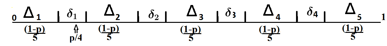
Figure 1: Partition of $[0,1)$ into $\Delta_{1},\delta_{1},\Delta_{2},\delta_{2},\ldots,\Delta_{5}$ for $r=5$.

We color the vertices of hypergraph $H$ according to the following Algorithm 1, which consists of two stages.

• First, each $v\in\Delta_{i}$ is colored with color $i$, $i=1,\ldots,r$

• Then, moving with growth of weight, we color a vertex $v\in\delta_{i}$ with color $i$ if such assignment does not create a monochromatic edge in the current coloring. Otherwise we color $v$ with color $i+1$.

Let $C^{0}$ denote the random coloring obtained after the consideration of all the vertices.

3.1 Analysis of Algorithm 1

Suppose that Algorithm 1 fails to produce a proper coloring and there is a monochromatic edge $A$ in the initial coloring $C^{0}$. Let $i\in\{1,2,...,r\}$ denote the color of $A$ and let $v_{A}$ be the first vertex of $A$. We note that $v_{A}$ could receive color $i$ only in two cases: either $v_{A}\in\Delta_{i}$ or $v_{A}\in\delta_{i-1}$. In the second case there exists an edge $B$, such that $v_{A}$ is the last vertex of $B$ and the remaining vertices of $B$ were colored with color $(i-1)$. In this situation we say that the pair $(A,B)$ is conflicting.

For the first vertex $v_{B}$ of the edge $B$ we also have an alternative: either $v_{B}\in\Delta_{i-1}$ or $v_{B}\in\delta_{i-2}$ and there exists an edge $C$ such that $v_{B}$ is the last vertex of $C$ and the remaining vertices of $C$ are colored with color $(i-2)$. Repeating the above arguments, we obtain a construction, called an ordered $k$-chain for color $i$. It is an edge sequence $H^{\prime}=(C_{1},...,C_{k-1}=B,C_{k}=A)$ such that the first vertex of $C_{1}$ belongs to the subinterval $\Delta_{i-k+1}$, and for every $j=2,...,k$, pair $(C_{j-1},C_{j})$ is conflicting.

Let us make some important notes concerning ordered chains.

1. The case of ordered $1$-chain corresponds to the case when $v_{A}\in\Delta_{i}$.

2. The last vertex of the edge $C_{k}=A$ belongs to the subinterval $\Delta_{i}$ (otherwise we should prefer the color $i+1$).

3. Every pair $(C_{j-1},C_{j})$ has exactly one vertex in common and this vertex belongs to $\delta_{j-1}$.

Summarizing the above, we can say that

Claim 1.

If for injective $\sigma:V\to[0;1)$ and for each color $i\in\{1,2,...,r\}$, there are no ordered chains then Algorithm 1 produces a proper coloring.

3.2 Auxiliary claims concerning ordered $k$-chains

Lemma 1.

The number of configurations in the hypergraph $H$ that can form an ordered $k$-chain is at most $2\binom{|E|}{k}$.

Proof.  Let us take an arbitrary unordered family of $k$ edges of $H$, $A_{1},\ldots,A_{k}$. This can be made by at most $\binom{|E|}{k}$ ways. If this set can form a chain, say, $(A_{1},\ldots,A_{k})$, then any successive two edges have exactly one common vertex and the remaining pairs do not intersect. So, there is only one more possible chain $(A_{k},\ldots,A_{1})$. $\Box$

Lemma 2.

Suppose $k\geq 1$ and let $H^{\prime}=(C_{1},\ldots,C_{k})$ be an ordered $k$-tuple of edges in the hypergraph $H$. Then the probability that $H^{\prime}$ forms an ordered $k$-chain for color $i$ does not exceed

$$2\left(\frac{\ln n}{n}\right)^{\frac{k(r-1)}{r}}r^{-(n-1)k-1}.$$

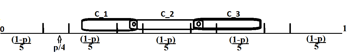
Figure 2: Ordered $3$-chain for color $4$

Proof.  Suppose $k\geq 2$. Let $v_{j}=C_{j}\cap C_{j+1}$ denote a common vertex of $C_{j}$ and $C_{j+1}$, $j=1,\ldots,k-1$, i.e. the vertex $v_{j}$ is the last vertex of the edge $C_{j}$ and is the first vertex of the edge $C_{j+1}$. Obviously, $v_{j}\in\delta_{i-k+j}$, $j=1,\ldots,k-1$. Let us also denote $\delta_{j}=[\alpha_{j},\beta_{j})$, $\beta_{j}-\alpha_{j}=p/(r-1)$.

So, for given weights $\sigma(v_{j})=x_{j}$, $j=1,\ldots,k-1$, the event that $H^{\prime}$ forms an ordered $k$-chain for color $i$, can be described as follows:

• every vertex $w\in C_{1}\setminus\{v_{1}\}$ should belong to the subinterval $\Delta_{i-k+1}\sqcup[\alpha_{i-k+1},x_{1})$;

• every vertex $w\in C_{j}\setminus(\{v_{j},v_{j-1}\})$, $j=2,\ldots,k-1$, should belong to the subinterval $[x_{j-1},\beta_{i-k+j-1})\sqcup\Delta_{i-k+j}\sqcup[\alpha_{i-k+j},x_{j})$;

• every vertex $w\in C_{k}\setminus\{v_{k-1}\}$ should belong to the subinterval $[x_{k-1},\beta_{i-1})\sqcup\Delta_{i}$.

The weights are independent, so denoting $y_{j}=x_{j}-\alpha_{i-k+j}$, we obtain the following estimate for the conditional probability:

$$\left(\frac{1-p}{r}+y_{1}\right)^{n-1}\times\left(\frac{1-p}{r}+y_{2}+\frac{p}{r-1}-y_{1}\right)^{n-2}\times\ldots\times$$

$$\times\left(\frac{1-p}{r}+y_{k-1}+\frac{p}{r-1}-y_{k-2}\right)^{n-2}\times\left(\frac{1-p}{r}+\frac{p}{r-1}-y_{k-1}\right)^{n-1}\leq$$

$$\leq\text{|take out the factor $r^{-k(n-2)-2}$ and use the estimate $(1+y)^{s}\leq\exp\{ys\}$}|\leq$$

$$\leq r^{-k(n-2)-2}\exp\{(n-1)\left(-p+ry_{1}\right)+(n-2)\left(-p+ry_{2}-ry_{1}+pr/(r-1)\right)+\ldots+$$

$$+(n-2)\left(-p+ry_{k-1}-ry_{k-2}+pr/(r-1)\right)+(n-1)\left(-p+pr/(r-1)-ry_{k-1}\right)\}\leq$$

$$\leq\text{|since $0\leq y_{j}\leq p/(r-1)$|}\leq$$

$$\leq r^{-k(n-2)-2}e^{(n-2)\left(-pk+\frac{(k-1)pr}{r-1}\right)}\cdot e^{\frac{2p}{r-1}}.$$

To obtain the final estimate, we have to integrate over $(y_{1},\ldots\,y_{k-1})\in[0,p/(r-1)]^{k-1}$ and substitute $p$ from (4). Thus, the probability under the consideration does not exceed

$$\left(\frac{p}{r-1}\right)^{k-1} r^{-k(n-2)-2}e^{(n-2)\left(-pk+\frac{(k-1)pr}{r-1}\right)}\cdot e^{\frac{2p}{r-1}}\leq$$

$$\leq\left|\text{since $e^{2p/(r-1)}\leq 2$ and $(-pk+(k-1)pr/(r-1))=\left(-1+\frac{k}{r}\right)\frac{\ln\left(\frac{n}{\ln n}\right)}{n}$}\right|\leq$$

$$\leq r^{-k(n-1)-1}\left(\frac{\ln n}{n}\right)^{k-1}\cdot e^{\left(-1+\frac{k}{r}\right)\ln\left(\frac{n}{\ln n}\right)}\cdot 2\leq$$

$$\leq 2\left(\frac{\ln n}{n}\right)^{\frac{k(r-1)}{r}}r^{-(n-1)k-1}.$$

If $k=1$ then every vertex of $C_{1}$ should belong to $\Delta_{i}$, so the probability does not exceed

$$\left(\frac{1-p}{r}\right)^{n}\leq\left(\frac{\ln n}{n}\right)^{\frac{r-1}{r}}r^{-n}.$$

$\Box$

3.3 Outcome of Algorithm 1

Lemmas 1 and 2 immediately imply the following statement.

Lemma 3.

The probability that a monochromatic edge occurs in the random coloring $C^{0}$ does not exceed $0.04e$.

Proof.  Lemma 1 estimates the number of possible configurations that can form an ordered $k$-chain and Lemma 2 does the same for the probability that a $k$-chain happens for a given color $i$. Bringing them together, we obtain that the required probability does not exceed

$$\sum_{k=1}^{r}2\binom{|E|}{k}\cdot 2r\left(\frac{\ln n}{n}\right)^{\frac{k(r-1)}{r}}\left(\frac{1}{r}\right)^{(n-1)k+1}\leq 4\sum_{k=1}^{\infty}\frac{(0.01)^{k}}{k!}\leq 0.04\cdot\sum_{k=1}^{\infty}\frac{1}{k!}<0.04e.$$

$\Box$

3.4 Some auxiliary claims concerning color classes

Let us return to the analysis of Algorithm 1:

• First, each $v\in\Delta_{i}$ is colored with color $i$, $i=1,\ldots,r$

• Then, moving with growth of weight, we color a vertex $v\in\delta_{i}$ with color $i$ if such assignment does not create a monochromatic edge in the current coloring. Otherwise we color $v$ with color $i+1$.

Let $X(i)$ denote the number of vertices $v\in\delta_{i}$ which have been colored with color $i+1$ during the evaluation of Algorithm 1. In other words, $X(i)$ is equal to the number of vertices $v\in\delta_{i}$ which Algorithm 1 could not color with $i$. The following lemma provides an estimate of the expected values of $X(i)$ in terms of number of edges $|E|$.

Lemma 4.

Suppose that number of edges $|E|$ of $H$ is at most $0.01\left(\frac{n}{\ln n}\right)^{\frac{r-1}{r}}r^{n-1}$. Then

1. the expected value of $X(i)$ does not exceed $0.04e\cdot\frac{n}{r\ln n}$, $i=1,\ldots,r-1$;

2. with probability at least $(1-0.04e)$ every $X(i)$ does not exceed $\frac{n}{\ln n}$.

Proof.  Suppose that $v\in\delta_{i}$ was colored with color $i+1$ during the evaluation of Algorithm 1. Since the color $i$ was not allowed, there exists an edge $A$ such that if $v$ is colored with color $i$ then $A$ would become monochromatic of color $i$. This means that all the vertices in $A\setminus\{v\}$ have smaller weights than $v$ and have been colored with $i$ during Algorithm 1. Now we can consider the first vertex of $A$. The same argument as in the proof of Claim 1 provides a chain $(C_{1},\ldots,C_{k})$ such that

1. $C_{k}=A$.

2. Every pair $(C_{j},C_{j+1})$, $j=1,\ldots,k-2$, is a conflicting pair. A vertex $v_{j}=C_{j}\cap C_{j+1}$ belongs to $\delta_{i-k+j}$.

3. The first vertex of $C_{1}$ belongs to $\Delta_{i-k+1}$.

4. A pair $(C_{k-1},C_{k})$ has one common vertex $v_{k-1}\in\delta_{i-1}$.

5. The last vertex $v$ of the edge $C_{k}$ belongs to $\delta_{i}$.

Roughly speaking, the last property is the only difference with ordered $k$-chain for color $i$. We will say that in the situation described above the set of edges $(C_{1},\ldots,C_{k})$ forms an improper k-chain for color $i$.

Estimation of the probability almost repeats the argument in Lemma 2. Again we use the notation $\delta_{j}=[\alpha_{j},\beta_{j})$, $\beta_{j}-\alpha_{j}=p/(r-1)$. For given weights $\sigma(v_{j})=x_{j}$, $j=1,\ldots,k-1$, the event that $(C_{1},\ldots,C_{k})$ forms an improper ordered $k$-chain for color $i$, can be described as follows:

• every vertex $w\in C_{1}\setminus\{v_{1}\}$ should belong to the subinterval $\Delta_{i-k+1}\sqcup[\alpha_{i-k+1},x_{1})$;

• every vertex $w\in C_{j}\setminus(\{v_{j},v_{j-1}\})$, $j=2,\ldots,k-1$, should belong to the subinterval $[x_{j-1},\beta_{i-k+j-1})\sqcup\Delta_{i-k+j}\sqcup[\alpha_{i-k+j},x_{j})$;

• every vertex $w\in C_{k}\setminus\{v_{k-1}\}$ should belong to the subinterval $[x_{k-1},\beta_{i-1})\sqcup\Delta_{i}\sqcup\delta_{i}$.

The weights are independent, so denoting $y_{j}=x_{j}-\alpha_{i-k+j}$, we obtain the following estimate for the conditional probability:

$$\left(\frac{1-p}{r}+y_{1}\right)^{n-1}\times\left(\frac{1-p}{r}+y_{2}+\frac{p}{r-1}-y_{1}\right)^{n-2}\times\ldots\times$$

$$\times\left(\frac{1-p}{r}+y_{k-1}+\frac{p}{r-1}-y_{k-2}\right)^{n-2}\times\left(\frac{1-p}{r}+\frac{p}{r-1}-y_{k-1}+\frac{p}{r-1}\right)^{n-1}\leq$$

$$\leq\text{|take out the factor $r^{-k(n-2)-2}$ and use the estimate $(1+y)^{s}\leq\exp\{ys\}$}|\leq$$

$$\leq r^{-k(n-2)-2}e^{(n-1)\left(-p+ry_{1}\right)}e^{(n-2)\sum_{j=2}^{k-1}\left(-p+ry_{j}-ry_{j-1}+pr/(r-1)\right)}e^{(n-1)\left(-p+pr/(r-1)-ry_{k-1}+\frac{p}{r-1}\right)}\leq$$

$$+(n-2)\left(-p+ry_{k-2}-ry_{k-3}+pr/(r-1)\right)+(n-1)\left(-p+2pr/(r-1)-ry_{k-1}\right)\}=$$

$$=r^{-k(n-2)-2}e^{(n-2)\left(-pk+\frac{kpr}{r-1}\right)}\cdot e^{\frac{2pr}{r-1}-2p}\cdot e^{ry_{1}-ry_{k-1}}\leq$$

$$\leq|\text{since }0\leq y_{1}\leq p/(r-1)|\leq$$

$$\leq r^{-k(n-2)-2}e^{(n-2)\left(-pk+\frac{kpr}{r-1}\right)}\cdot e^{\frac{3p}{r-1}}=$$

$$=r^{-k(n-2)-2}e^{\frac{npk}{r-1}-\frac{2pk}{r-1}}\cdot e^{\frac{3p}{r-1}}\leq r^{-k(n-2)-2}e^{\frac{npk}{r-1}}\cdot e^{\frac{p}{r-1}}.$$

To obtain the final estimate, we have to integrate over $(y_{1},\ldots\,y_{k-1})\in[0,p/(r-1)]^{k-1}$ and substitute $p$ from (4). Thus, the probability under the consideration does not exceed

$$\left(\frac{p}{r-1}\right)^{k-1} r^{-k(n-2)-2}e^{\frac{npk}{r-1}}\cdot e^{\frac{p}{r-1}}\leq$$

$$\leq\left|\text{since $e^{p/(r-1)}\leq 2$}\right|\leq$$

$$\leq r^{-k(n-1)-1}\left(\frac{\ln n}{n}\right)^{k-1}\cdot\left(\frac{n}{\ln n}\right)^{\frac{k}{r}}\cdot 2=$$

$$=2\left(\frac{\ln n}{n}\right)^{\frac{k(r-1)}{r}-1}r^{-(n-1)k-1}.$$

So, the expected value of $X(i)$ can be estimated as follows:

$${\sf E}X(i)\leq\sum_{k=1}^{r}2{|E|\choose k}\cdot 2\left(\frac{\ln n}{n}\right)^{\frac{k(r-1)}{r}-1}\left(\frac{1}{r}\right)^{(n-1)k+1}\leq\frac{4n}{r\ln n}\sum_{k=1}^{\infty}\frac{(0.01)^{k}}{k!}\leq\frac{0.04en}{r\ln n}.$$

The last statement of Lemma 4 obviously follows from Markov inequality:

$$\mathop{\kern 0.0pt\mathsf{P}}\nolimits\left(\exists i:X(i)>\frac{n}{\ln n}\right)\leq r\frac{{\sf E}X(i)}{\frac{n}{\ln n}}\leq 0.04e.$$

$\Box$

Let $K_{1},\ldots,K_{r}$ denote the color classes of the initial coloring $C^{0}$. For every color class $K_{\alpha}$, let us define nonnegative integers $ex_{\alpha}$ and $sh_{\alpha}$, where $ex_{\alpha}$ stands for the excess value, i.e. a positive difference between number of vertices of the color ${\alpha}$ and $m/r$, and $sh_{\alpha}$ stands for the shortage value. Formally,

$$ex_{\alpha}=\begin{cases}|K_{\alpha}|-\frac{m}{r},&\mbox{ if }|K_{\alpha}|-\frac{m}{r}>0;\\ 0,&\mbox{otherwise};\end{cases}$$

$$sh_{\alpha}=\begin{cases}\frac{m}{r}-|K_{\alpha}|,&\mbox{ if }\frac{m}{r}-|K_{\alpha}|>0;\\ 0,&\mbox{otherwise}.\end{cases}$$

The following lemma estimates the value of excesses and shortages.

Lemma 5.

With probability at least $1/2-0.04e$ the following conditions hold simultaneously:

1. the first $r-1$ colors are in excess, i.e. the sizes if their color classes are at least $m/r$,

2. for each color $i$ excess value $ex_{i}\leq\frac{p}{r(r-1)}m+\sqrt{\frac{13m\ln r}{r}}+\frac{n}{\ln n}$.

Proof.  Let $Z(i)$ denote the number of vertices, which belong to subinterval $\Delta_{i-1}\cup\delta_{i}$. Any such random variable has the binomial distribution $Bin(m,\frac{1-p}{r}+\frac{p}{r-1})$ with mean $m\left(\frac{1}{r}+\frac{p}{r(r-1)}\right)$. Then the number of vertices colored with color $i$ in $C^{0}$ is equal to

$$Z(i)-X(i)+X(i-1).$$

We use Chernoff’s inequality which states that for any random binomial variable $\xi$ and any $z>0$, it holds that

$$\mathop{\kern 0.0pt\mathsf{P}}\nolimits(\xi<{\sf E}\xi-z)\leq\exp\left(-\frac{z^{2}}{2{\sf E}\xi}\right).$$

$$\mathop{\kern 0.0pt\mathsf{P}}\nolimits(\xi>{\sf E}\xi+z)\leq\exp\left(-\frac{z^{2}}{2({\sf E}\xi+z/3)}\right).$$

Let us apply it for $\xi=Z(i)$ and $z=\sqrt{\frac{13m\ln r}{r}}$. Due to the initial restrictions on the parameter $r$ we have that $z<m/(2r)$. Hence,

$$\mathop{\kern 0.0pt\mathsf{P}}\nolimits\left(\exists i:Z(i)>m\left(\frac{1-p}{r}+\frac{p}{r-1}\right)+z\right)\leq r\exp\left(-\frac{z^{2}}{2(2\frac{m}{r}+z/3)}\right)<$$

$$<r\exp\left(-\frac{z^{2}}{2\cdot\frac{13m}{6r}}\right)=r\exp\left(-3\ln r\right)=r^{-2}\leq 2^{-2}.$$

Similarly,

$$\mathop{\kern 0.0pt\mathsf{P}}\nolimits\left(\exists i:Z(i)<m\left(\frac{1-p}{r}+\frac{p}{r-1}\right)-z\right)\leq r^{-2}\leq 2^{-2}.$$

Then, with probability at least $1-0.04e-2^{-1}=1/2-0.04e$ the following conditions hold simultaneously:

$$\frac{p}{r(r-1)}m+\sqrt{\frac{13m\ln r}{r}}+\frac{n}{\ln n}\geq Z(i)-X(i)+X(i-1)$$

$$Z(i)-X(i)+X(i-1)\geq m\left(\frac{1-p}{r}+\frac{p}{r-1}\right)-\sqrt{\frac{13m\ln r}{r}}-\frac{n}{\ln n}=$$

$$=\frac{m}{r}+\frac{mp}{r(r-1)}-\sqrt{\frac{13m\ln r}{r}}-\frac{n}{\ln n}.$$

Hence, we have a desired upper bound on the excess value. Now notice that the first $(r-1)$ colors will be in excess if

$$\frac{mp}{r(r-1)}-\sqrt{\frac{13m\ln r}{r}}-\frac{n}{\ln n}=\frac{m\ln\left(\frac{n}{\ln n}\right)}{nr^{2}}-\sqrt{\frac{13m\ln r}{r}}-\frac{n}{\ln n}>0$$

Since $m>\frac{n^{2}(r-1)}{2\ln n}$, the last inequality holds for $r<\sqrt[3]{\ln n}$ and all large enough $n$. $\Box$

4 Construction of an equitable coloring

The final part of our work is devoted to restoring the color balance in the coloring $C^{0}$. According to Lemma 5 we know that with positive probability first $(r-1)$ color classes are in excess, i.e. their sizes are at least $m/r$. Therefore, we are going to recolor some vertices from the color classes $K_{1},...,K_{r-1}$ with color $r$ keeping the lack of the monochromatic edges.

Now we formalize our idea: we want show that in every $\Delta_{i}$, $i=1,\ldots,r-1$, it is possible to choose a vertex subset $W_{i}$ of size $ex_{i}$ such that the recoloring of sets $W_{i}$ with color $r$ does not create monochromatic edges. If such choice of subsets is possible then we will be able to correct the color balance.

4.1 Proof of the existence of sets $W_{i}$

Before we introduce the proof, let us simplify the next sum by one symbol and introduce a new parameter:

$$q=\frac{mp}{r(r-1)}+2\sqrt{\frac{13m\ln r}{r}}+\frac{r+1}{r}\frac{n}{\ln n}$$ (5)

Now we are ready to establish the existence (with positive probability) of the required collection of sets. We consider a random subset $V_{i}$, $i=1\ldots,r-1$, constructed according to the binomial scheme: with probability

$$\tilde{p}=q\times\frac{r}{(1-p)m}$$ (6)

every vertex of $\Delta_{i}$ is included to $V_{i}$ independently of each other.

Which vertices of $V_{i}$ are not suitable to include in $W_{i}$? Clearly, we do not want to take the vertices whose recoloring with color $r$ can create monochromatic edges of color $r$. This situation happens when there is an edge $A$ and a subset of vertices $U(A)\subset A$ such that

• all vertices in $A\setminus U(A)$ are colored with $r$ in the coloring $C^{0}$;

• all vertices in $U(A)$ belong to $\cup_{i=1}^{r-1}V_{i}$.

In this case we do not want to take $U(A)$ completely into $\cup_{i=1}^{r-1}W_{i}$. Such an edge $A$ is called dangerous. Let $Q$ denote the number of dangerous edges. So, to establish the existence of the required sets $W_{1},\ldots,W_{r-1}$ it suffices to show that with positive probability the following conditions hold: for any $i=1,\ldots,r-1$,

$$|V_{i}|\geq Q+ex_{i}.$$

We have already shown that with positive probability $ex_{i}\leq\frac{p}{r(r-1)}m+\sqrt{\frac{13m\ln r}{r}}+\frac{n}{\ln n}$. So, it remains only to estimate $Q$ and the cardinalities $|V_{i}|$.

Let us start with $|V_{i}|$. It is clear from the construction that $|V_{i}|$ is a binomial random variable $Bin(m,q/m)$. So, by using Chernoff inequality, we get

$${\sf P}\left(|V_{i}|<q-\sqrt{\frac{13m\ln r}{r}}\right) \leq e^{-\frac{\frac{13m\ln r}{r}}{2q}}\leq$$

$$\leq|\mbox{since }q<\frac{2mp}{r(r-1)}|\leq$$

$$\leq e^{-(13)/4\cdot(r-1)(\ln r)p^{-1}}\leq r^{-p^{-1}}<r^{-10}$$

for all large enough $n$. Hence, with probability at least $1-r^{-9}\geq 1-2^{-9}$ every $|V_{i}|$ is at least

$$|V_{i}|\geq q-\sqrt{\frac{13m\ln r}{r}}=\frac{mp}{r(r-1)}+\sqrt{\frac{13m\ln r}{r}}+\frac{r+1}{r}\frac{n}{\ln n}.$$

4.2 Dangerous edges and $k$-complex ordered chains

Suppose that $A$ is a dangerous edge. Let us denote $A^{\prime}=A\setminus U(A)$. Then $A^{\prime}$ can be considered as a monochromatic ‘‘pseudo-edge’’ of color $r$ during the evaluation of Algorithm 1. Hence, we can construct an ordered $k$-chain $H^{\prime}=(C_{1},...,C_{k}=A^{\prime})$ for color $r$ with the ‘‘pseudo-edge’’ $A^{\prime}$ as the last edge in the chain. Note that $A^{\prime}$ should be contained in $\delta_{r-1}\cup\Delta_{r}$ ($A^{\prime}$ is colored with $r$ in $C^{0}$) and, vice versa, none of the vertices of $U(A)$ can be contained in $\delta_{r-1}\cup\Delta_{r}$, so $A^{\prime}=A\cap(\delta_{r-1}\cup\Delta_{r})$. Now we can described a $k$-complex ordered chain $H^{\prime\prime}=(C_{1},...,C_{k}=A)$ as follows:

• $H^{\prime}=(C_{1},...,C_{k-1},A^{\prime})$, where $A^{\prime}=A\cap(\delta_{r-1}\cup\Delta_{r})$, is an ordered $k$-chain for color $r$ with pseudo-edge $A^{\prime}$;

• all vertices in $U(A)=A\setminus A^{\prime}$ belong to $\cup_{i=1}^{r-1}V_{i}$.

• every vertex $w\in A\cap C_{j}$ should belong to $V_{r-k+j}$, $j\in\{1,...,k-2\}$;

• every vertex $w\in(A\setminus A^{\prime})\cap C_{k-1}$ should belong to $V_{r-1}$.

Lemma 6.

For given edge $A$, the number of configurations that can form a $k$-complex ordered chain $k\geq 2$ in the hypergraph $H$ with $A$ as the last edge is at most $2\binom{|E|}{k-1}$.

Proof.  Let us take an arbitrary unordered family of $k-1$ edges of $H$, say, $A_{1},\ldots,A_{k-1}$. This can be done in at most $\binom{|E|}{k-1}$ ways. If $A_{1},\ldots,A_{k-1}$ can form a chain then there are only two candidates for the the first edge in the chain (it should have only one common vertex with the union of others). After choosing the first edge the order in the chain is defined uniquely. $\Box$

Lemma 7.

With probability at least $(1-0.02)$ the number of dangerous edges $Q$ does not exceed $\frac{1}{r}\left(\frac{n}{\ln n}\right)$

Proof.  Suppose $k\geq 2$. We want to estimate the probability that an ordered $k$-tuple of edges $H^{\prime\prime}=(C_{1},\ldots,C_{k}=A)$ is a $k$-complex ordered chain. For any $j=1,\ldots,k-2$, we denote

$$v_{j}=C_{j}\cap C_{j+1}\mbox{ and }s_{j}=|A\cap C_{j}|.$$

Then we choose a vertex $v_{j}\in C_{k-1}\cap A$ to be the unique common vertex of $A^{\prime}$ and $C_{k-1}$ and denote $s_{k-1}=|A\cap C_{k-1}|-1$. Denote also

$$s=s_{1}+...+s_{k-1}.$$

Recall that we use the notation $\delta_{j}=[\alpha_{j},\beta_{j})$. Thus, for given weights $\sigma(v_{j})=x_{j}\in\delta_{r-k+j}$, $j=1,\ldots,k-1$, the event that $H^{\prime\prime}$ forms a $k$-complex ordered chain for color $r$, can be described as follows:

• every vertex $w\in C_{1}\setminus\{v_{1}\}$ should belong to the subinterval $\Delta_{r-k+1}\sqcup[\alpha_{r-k+1},x_{1})$;

• every vertex $w\in C_{j}\setminus(\{v_{j}\cup v_{j-1}\})$, $j=2,\ldots,k-1$, should belong to the subinterval $[x_{j-1},\beta_{r-k+j-1})\sqcup\Delta_{r-k+j}\sqcup[\alpha_{r-k+j},x_{j})$;

• every vertex $w\in A\setminus(\{v_{k-1}\}\cup C_{1}\cup\ldots\cup C_{k-1})$ either belongs to the subinterval $[x_{k-1},\beta_{r-1})\sqcup\Delta_{r}$ or belongs to some $V_{i}$, $i=1,\ldots,r-1$;

• every vertex $w\in(A\cap C_{j})$ should belong to $V_{r-k+j}$, $j\in\{1,...,k-2\}$.

• every vertex $w\in(A\cap C_{k-1})\setminus\{v_{k-1}\}$ should belong to $V_{r-1}$.

Note that for every vertex $w$, ${\sf P}(w\in V_{i})=(1-p)/r\cdot\widetilde{p}=q/m$ and this event is independent of the weights of other vertices.

As before, let $y_{j}=x_{j}-\alpha_{i-k+j}$. Now we are ready to estimate the conditional probability of event the $k$-complex chain occur given weights $x_{j}$ are fixed:

$$\left(\frac{q}{m}\right)^{s}\left(\frac{1-p}{r}+y_{1}\right)^{n-1-s_{1}}\times\left(\frac{1-p}{r}+y_{2}+\frac{p}{r-1}-y_{1}\right)^{n-2-s_{2}}\times\ldots\times$$

$$\times\left(\frac{1-p}{r}+y_{k-1}+\frac{p}{r-1}-y_{k-2}\right)^{n-2-s_{k-1}}\times\left(\frac{1-p}{r}+\frac{p}{r-1}-y_{k-1}+\frac{(r-1)q}{m}\right)^{n-1-s}\leq$$

(take out the factor $r$)

$$\leq r^{-k(n-2)-2+s}\left(\frac{qr}{m}\right)^{s}(1-p+ry_{1})^{n-1-s_{1}}\left(1+\frac{p}{r-1}+ry_{2}-ry_{1}\right)^{n-2-s_{2}}\times\ldots\times$$

$$\times\left(1+\frac{p}{r-1}+ry_{k-1}-ry_{k-2}\right)^{n-2-s_{k-1}}\left(1+\frac{p}{r-1}-ry_{k-1}+\frac{(r-1)rq}{m}\right)^{n-1-s}\leq$$

$$\leq\mbox{|since any expression in the brackets among the last three is at least $1-p$|}\leq$$

$$\leq r^{-k(n-2)-2+s}\left(\frac{qr}{m}\right)^{s}(1-p+ry_{1})^{n-1}\times$$

$$\times\left(1+\frac{p}{r-1}+ry_{2}-ry_{1}\right)^{n-2}\times\ldots\times\left(1+\frac{p}{r-1}+ry_{k-1}-ry_{k-2}\right)^{n-2}\times$$

$$\times\ldots\times\left(1+\frac{p}{r-1}-ry_{k-1}+\frac{r(r-1)q}{m}\right)^{n-1}\times\frac{1}{(1-p)^{s_{1}+...s_{k-1}+s}}\leq$$

$$\leq r^{-k(n-2)-2+s}\left(\frac{qr}{m(1-p)^{2}}\right)^{s}\times$$

$$\times\exp\left\{-p(n-1)+\frac{p(n-1)}{r-1}(k-1)+ry_{1}+\frac{r(r-1)(n-1)q}{m}\right\}.$$

Let us analyze the obtained expression. Note that $q\leq 2mp/(r-1)r$ and $(1-p)^{2}>1/2$, so (4) implies that

$$\left(\frac{qr}{m(1-p)^{2}}\right)^{s}\leqslant\left(\frac{4p}{r-1}\right)^{s}\leqslant\left(\frac{4\ln n}{nr}\right)^{s}.$$

Then since $y_{1}\leqslant\frac{p}{r-1}$

$$-p(n-1)+\frac{p(n-1)}{r-1}(k-1)+ry_{1}\leqslant 3p-pn+\frac{pn}{r-1}(k-1)=3p+\frac{k-r}{r-1}\ln\left(\frac{n}{\ln n}\right)^{\frac{r-1}{r}}.$$

Finally, (5) yields that

$$\frac{r(r-1)(n-1)q}{m}\leqslant\left(\frac{mp}{r(r-1)}+2\sqrt{\frac{13m\ln r}{r}}+\frac{r+1}{r}\frac{n}{\ln n}\right)\times\frac{r(r-1)(n-1)}{m}=$$

$$=p(n-1)+\frac{(r^{2}-1)n(n-1)}{m\ln n}+2\sqrt{\frac{13r\ln r}{m}}r(n-1)\leq$$

$$\leq|\mbox{using \eqref{vert_bound_new}}|\leq p(n-1)+2(r+1)+2\sqrt{26\ln r\ln n}\cdot r\leq$$

$$\leq p(n-1)+\frac{1}{r}\ln\frac{n}{\ln n}$$

for $r<(\ln n)^{1/5}$ and all large enough $n$. Since $pn=\frac{r-1}{r}\ln\frac{n}{\ln n}$, we obtain the following estimate for the conditional probability:

$$r^{-k(n-2)-2+s}\left(\frac{4\ln n}{nr}\right)^{s}e^{3p}\left(\frac{n}{\ln n}\right)^{\frac{k-r}{r}+1}=r^{-k(n-2)-2}\left(\frac{4\ln n}{n}\right)^{s}e^{3p}\left(\frac{n}{\ln n}\right)^{\frac{k}{r}}.$$

To obtain the final estimate, we have to integrate over the weights $y_{1},\ldots\,y_{k-1}$ (factor $\left(p/(r-1)\right)^{k-1}$) and sum up over all possible variants for the vertex $v_{k-1}$ (at most $s+1$ ways). Thus, we get the bound

$$r^{-k(n-2)-2}\left(\frac{4\ln n}{n}\right)^{s}e^{3p}\left(\frac{n}{\ln n}\right)^{\frac{k}{r}}\left(\frac{p}{r-1}\right)^{k-1}(s+1)\leq$$

$$\leq(s+1)\left(\frac{4\ln n}{n}\right)^{s}r^{-k(n-1)-1}e^{3p}\left(\frac{n}{\ln n}\right)^{\frac{k}{r}-k+1}.$$

Clearly, the bound is maximized for $s=1$.

If $k=1$ then the expected value of the number of dangerous edges can be estimated without complex ordered chains.

$$\left(\frac{1-p}{r}+\frac{(r-1)q}{m}\right)^{n}\leq r^{-n}e^{-pn+\frac{(r-1)qrn}{m}}\leq r^{-n}e^{\frac{1}{r}\ln\frac{n}{\ln n}}.$$

So, we are ready to estimate the expected value of the number of dangerous edges. Lemma 6 and the initial condition on the number edges imply that

$${\sf E}Q\leq |E|r^{-n}e^{\frac{1}{r}\ln\frac{n}{\ln n}}+|E|\sum_{k=2}^{r}2{|E|\choose k-1}r^{-k(n-1)-1}e^{3p}\left(\frac{n}{\ln n}\right)^{\frac{k}{r}-k+1}\leq$$

$$\leq 0.01\cdot r^{-1}\frac{n}{\ln n}+2e^{3p}r^{-1}\frac{n}{\ln n}\sum_{k=2}^{r}\frac{(0.01)^{k}}{(k-1)!}\leq$$

$$\leq\frac{n}{r\ln n}\left(0.01+0.02e^{3p}(e^{0.01}-1)\right)\leq 0.02\cdot\frac{n}{r\ln n}$$

By Markov inequality we can conclude that the number of dangerous edges $Q$ does not exceed $\frac{1}{r}\left(\frac{n}{\ln n}\right)$ with probability at least $1-0.02$. $\Box$

4.3 Completion of the proof of Theorem 1

Let us sum up.

1)We have shown that the probability that there are monochromatic edges in the coloring $C^{0}$, does not exceed $0.04e$ (Lemma 3).

2) With probability at least $1/2-0.04e$ the first $r-1$ colors are in excess and for each color $i$, the excess value $ex_{i}\leq\frac{p}{r(r-1)}m+\sqrt{\frac{13m\ln r}{r}}+\frac{n}{\ln n}$. (Lemma 5).

3) The probability that the number of dangerous edges is at least $\frac{1}{r}\left(\frac{n}{\ln n}\right)$ does not exceed $0.02$ (Lemma 7).

4) With probability at least $1-2^{-9}$ every $V_{i}$ has cardinality at least $\frac{mp}{r(r-1)}+\sqrt{\frac{13m\ln r}{r}}+\frac{r+1}{r}\left(\frac{n}{\ln n}\right)$.

So, with probability at least $1/2-(0.04e+0.04e+0.02+2^{-9})>0$ there are no monochromatic edges and for every color $i$, the following relation holds:

$$ex_{i}+Q\leq|V_{i}|.$$

Hence, we can choose the required sets $W_{i}$ of size $ex_{i}$ and safely recolor them with color $r$ to obtain an equitable coloring of $H$. Theorem 1 is proved.

5 Acknowledgements

The work is supported by the grant of the President of Russian Federation no. MD-757.2019.1.

References

- [1] D. Cherkashin, J. Kozik, ‘‘A note on random greedy coloring of uniform hypergraphs’’, Random Structures and Algorithms, 47:3 (2015), 407–413.
- [2] A.V. Kostochka, ‘‘Color-Critical Graphs and Hypergraphs with Few Edges: A Survey’’, In: More Sets, Graphs and Numbers, Bolyai Society Mathematical Studies, 15, Springer, 2006, 175–198.
- [3] I.A. Akolzin, D.A. Shabanov, ‘‘Colorings of hypergraphs with large number of colors’’, Discrete Mathematics, 339:12 (2016), 3020–3031.
- [4] D. Cherkashin, ‘‘Note on panchromatic colorings’’, Discrete Mathematics, 341:13, (2018), 652–657.
- [5] J. Kozik, D.A. Shabanov, ‘‘Improved algorithms for colorings of simple hypergraphs and applications’’, Journal of Combinatorial Theory, Series B, 116 (2016), 312–332.
- [6] A. Kupavskii, D. Shabanov, ‘‘Colourings of uniform hypergraphs with large girth and applications’’, Combinatorics, Probability and Computing, 27:2 (2018), 245–273.
- [7] M. Akhmejanova, D. Shabanov, ‘‘Colorings of b-simple hypergraphs’’, Electronic Notes in Discrete Mathematics, 61 (2017), 29–35.
- [8] M. Dyer, A. Frieze, C. Greenhill, ‘‘On the chromatic number of a random hypergraph’’, Journal of Combinatorial Theory, Series B, 113 (2015), 68–122.
- [9] D.A. Shabanov, ‘‘On the concentration of the chromatic number of a random hypergraph’’, Doklady Mathematics, 96:1 (2017), 321–325.
- [10] P. Ayre, A. Coja-Oghlan, C. Greenhill, ‘‘Hypergraph coloring up to condensation’’, Random Structures and Algorithms, https://doi.org/10.1002/rsa.20824.
- [11] D.A. Kravtsov, N.E. Krokhmal, D.A. Shabanov, ‘‘Panchromatic 3-colorings of random hypergraphs’’, European Journal of Combinatorics, 78 (2019), 28–43.
- [12] A. Hajnal, E. Szemeredi, ‘‘Proof of a conjecture of P. Erdős’’, Combinatorial theory and its applications, North-Holland, London, II (1969), 601–623
- [13] P. Erdős , ‘‘Theory of Graphs and Its Applications” (M. Fieldler, Ed.) Czech. Acad. Sci. Publ., Prague, 9 (1964), 159.
- [14] H. Kierstead, A. Kostochka, ‘‘A short proof of Hajnal-Szemerédi Theorem on equitable coloring’’, Combinatorics, Probability and Computing, 17:2 (2008), 265–270.
- [15] H. Kierstead, A. Kostochka, ‘‘An Ore-type theorem on equitable coloring’’, Journal of Combinatorial Theory, Series B, 98:1 (2008), 226–234.
- [16] H. Kierstead, A. Kostochka, M. Mydlarz, E. Szemerédi, ‘‘A fast algorithm for equitable coloring’’, Combinatorica, 30:2 (2010), 217–224
- [17] L. Lu, L. Székely, ‘‘Using Lovász Local Lemma in the space of random injections’’, Electronic Journal of Combinatorics, 13 (2007), Research paper 63.
- [18] P. Erdós and A. Hajnal, ‘‘On chromatic number of graphs and set systems’’, Acta Math. Acad. Sci. Hung., 17 (1966), 61–99.
- [19] A. Pluhár, ‘‘Greedy colorings for uniform hypergraphs’’, Random Structures Algorithms, 35:2 (2009), 216–221.