Transfer Learning Between Related Tasks
Using Expected Label Proportions

Abstract

Deep learning systems thrive on abundance of labeled training data but such data is not always available, calling for alternative methods of supervision. One such method is expectation regularization (XR) Mann and McCallum (2007), where models are trained based on expected label proportions. We propose a novel application of the XR framework for transfer learning between related tasks, where knowing the labels of task A provides an estimation of the label proportion of task B. We then use a model trained for A to label a large corpus, and use this corpus with an XR loss to train a model for task B. To make the XR framework applicable to large-scale deep-learning setups, we propose a stochastic batched approximation procedure. We demonstrate the approach on the task of Aspect-based Sentiment classification, where we effectively use a sentence-level sentiment predictor to train accurate aspect-based predictor. The method improves upon fully supervised neural system trained on aspect-level data, and is also cumulative with LM-based pretraining, as we demonstrate by improving a BERT-based Aspect-based Sentiment model.

1 Introduction

Data annotation is a key bottleneck in many data driven algorithms. Specifically, deep learning models, which became a prominent tool in many data driven tasks in recent years, require large datasets to work well. However, many tasks require manual annotations which are relatively hard to obtain at scale. An attractive alternative is lightly supervised learning Schapire et al. (2002); Jin and Liu (2005); Chang et al. (2007); Graça et al. (2007); Quadrianto et al. (2009a); Mann and McCallum (2010a); Ganchev et al. (2010); Hope and Shahaf (2016), in which the objective function is supplemented by a set of domain-specific soft-constraints over the model’s predictions on unlabeled data. For example, in label regularization Mann and McCallum (2007) the model is trained to fit the true label proportions of an unlabeled dataset. Label regularization is special case of expectation regularization (XR) Mann and McCallum (2007), in which the model is trained to fit the conditional probabilities of labels given features.

In this work we consider the case of correlated tasks, in the sense that knowing the labels for task A provides information on the expected label composition of task B. We demonstrate the approach using sentence-level and aspect-level sentiment analysis, which we use as a running example: knowing that a sentence has positive sentiment label (task A), we can expect that most aspects within this sentence (task B) will also have positive label. While this expectation may be noisy on the individual example level, it holds well in aggregate: given a set of positively-labeled sentences, we can robustly estimate the proportion of positively-labeled aspects within this set. For example, in a random set of positive sentences, we expect to find 90% positive aspects, while in a set of negative sentences, we expect to find 70% negative aspects. These proportions can be easily either guessed or estimated from a small set.

We propose a novel application of the XR framework for transfer learning in this setup. We present an algorithm (Sec 3.1) that, given a corpus labeled for task A (sentence-level sentiment), learns a classifier for performing task B (aspect-level sentiment) instead, without a direct supervision signal for task B. We note that the label information for task A is only used at training time. Furthermore, due to the stochastic nature of the estimation, the task A labels need not be fully accurate, allowing us to make use of noisy predictions which are assigned by an automatic classifier (Sections 3.1 and 4). In other words, given a medium-sized sentiment corpus with sentence-level labels, and a large collection of un-annotated text from the same distribution, we can train an accurate aspect-level sentiment classifier.

The XR loss allows us to use task A labels for training task B predictors. This ability seamlessly integrates into other semi-supervised schemes: we can use the XR loss on top of a pre-trained model to fine-tune the pre-trained representation to the target task, and we can also take the model trained using XR loss and plentiful data and fine-tune it to the target task using the available small-scale annotated data. In Section 5.3 we explore these options and show that our XR framework improves the results also when applied on top of a pre-trained Bert-based model Devlin et al. (2018).

Finally, to make the XR framework applicable to large-scale deep-learning setups, we propose a stochastic batched approximation procedure (Section 3.2). Source code is available at https://github.com/MatanBN/XRTransfer.

2 Background and Related Work

2.1 Lightly Supervised Learning

An effective way to supplement small annotated datasets is to use lightly supervised learning, in which the objective function is supplemented by a set of domain-specific soft-constraints over the model’s predictions on unlabeled data. Previous work in lightly-supervised learning focused on training classifiers by using prior knowledge of label proportions (Jin and Liu, 2005; Chang et al., 2007; Musicant et al., 2007; Mann and McCallum, 2007; Quadrianto et al., 2009b; Liang et al., 2009; Ganchev et al., 2010; Mann and McCallum, 2010b; Chang et al., 2012; Wang et al., 2012; Zhu et al., 2014; Hope and Shahaf, 2016) or prior knowledge of features label associations (Schapire et al., 2002; Haghighi and Klein, 2006; Druck et al., 2008; Melville et al., 2009; Mohammady and Culotta, 2015). In the context of NLP, Haghighi and Klein (2006) suggested to use distributional similarities of words to train sequence models for part-of-speech tagging and a classified ads information extraction task. Melville et al. (2009) used background lexical information in terms of word-class associations to train a sentiment classifier. Ganchev and Das (2013); Wang and Manning (2014) suggested to exploit the bilingual correlations between a resource rich language and a resource poor language to train a classifier for the resource poor language in a lightly supervised manner.

2.2 Expectation Regularization (XR)

Expectation Regularization (XR) Mann and McCallum (2007) is a lightly supervised learning method, in which the model is trained to fit the conditional probabilities of labels given features. In the context of NLP, XR was used by Mohammady and Culotta (2015) to train twitter-user attribute prediction using hundreds of noisy distributional expectations based on census demographics. Here, we suggest using XR to train a target task (aspect-level sentiment) based on the output of a related source-task classifier (sentence-level sentiment).

Learning Setup

The main idea of XR is moving from a fully supervised situation in which each data-point $x_{i}$ has an associated label $y_{i}$, to a setup in which sets of data points $U_{j}$ are associated with corresponding label proportions $\mathbf{\tilde{p}_{j}}$ over that set.

Formally, let $X=\{x_{1},x_{2},\dots,x_{n}\}\subseteq{\mathcal{X}}$ be a set of data points, $\mathcal{Y}$ be a set of $|\mathcal{Y}|$ class labels, $U=\{U_{1},U_{2},\dots,U_{m}\}$ be a set of sets where $U_{j}\subseteq X$ for every $j\in\{1,2,\dots,m\}$, and let $\mathbf{\tilde{p}_{j}}\in R^{|\mathcal{Y}|}$ be the label distribution of set $U_{j}$. For example, $\mathbf{\tilde{p}_{j}}=\{.7,.2,.1\}$ would indicate that 70% of data points in $U_{j}$ are expected to have class 0, 20% are expected to have class 1 and 10% are expected to have class 2. Let $p_{\theta}(x)$ be a parameterized function with parameters $\theta$ from $\mathcal{X}$ to a vector of conditional probabilities over labels in $\mathcal{Y}$. We write $p_{\theta}(y|x)$ to denote the probability assigned to the $y$th event (the conditional probability of $y$ given $x$).

A typically objective when training on fully labeled data of $(x_{i},y_{i})$ pairs is to maximize likelihood of labeled data using the cross entropy loss,

$$L_{cross}(\theta)=-\sum\limits_{i}^{n}\log p_{\theta}(y_{i}|x_{i})$$

Instead, in XR our data comes in the form of pairs $(U_{j},\mathbf{\tilde{p}_{j}})$ of sets and their corresponding expected label proportions, and we aim to optimize $\theta$ to fit the label distribution $\mathbf{\tilde{p}_{j}}$ over $U_{j}$, for all $j$.

XR Loss

As counting the number of predicted class labels over a set $U$ leads to a non-differentiable objective, Mann and McCallum (2007) suggest to relax it and use instead the model’s posterior distribution $\mathbf{\hat{p}_{j}}$ over the set:

$$\mathbf{\hat{q}_{j}}(y)=\sum_{x\in U_{j}}p_{\theta}(y|x)$$ (1)

$$\mathbf{\hat{p}_{j}}(y)=\dfrac{\mathbf{\hat{q}_{j}}(y)}{\sum_{y^{\prime}}\mathbf{\hat{q}_{j}}(y^{\prime})}$$ (2)

where $\mathbf{q}(y)$ indicates the $y$th entry in $\mathbf{q}$. Then, we would like to set $\theta$ such that $\mathbf{\hat{p}_{j}}$ and $\mathbf{\tilde{p}_{j}}$ are close. Mann and McCallum (2007) suggest to use KL-divergence for this. KL-divergence is composed of two parts:

$$D_{KL}(\mathbf{\tilde{p}_{j}}||\mathbf{\hat{p}_{j}})=-\mathbf{\tilde{p}_{j}}\cdot\log\mathbf{\hat{p}_{j}}+\mathbf{\tilde{p}_{j}}\cdot\log\mathbf{\tilde{p}_{j}}$$

$$=H(\mathbf{\tilde{p}_{j}},\mathbf{\hat{p}_{j}})-H(\mathbf{\tilde{p}_{j}})$$

Since $H(\mathbf{\tilde{p}_{j}})$ is constant, we only need to minimize $H(\mathbf{\tilde{p}_{j}},\mathbf{\hat{p}_{j}})$, therefore the loss function becomes:

$$L_{XR}(\theta)=-\sum_{j=1}^{m}\mathbf{\tilde{p}_{j}}\cdot\log\mathbf{\hat{p}_{j}}$$ (3)

Notice that computing $\mathbf{\hat{q}_{j}}$ requires summation over $p_{\theta}(x)$ for the entire set $U_{j}$, which can be prohibitive. We present batched approximation (Section 3.2) to overcome this.

Temperature Parameter

Mann and McCallum (2007) find that XR might find a degenerate solution. For example, in a three class classification task, where $\tilde{p}_{j}=\{.5,.35,.15\}$, it might find a solution such that $\hat{p}_{\theta}(y)=\{.5,.35,.15\}$ for every instance, as a result, every instance will be classified the same. To avoid this, Mann and McCallum (2007) suggest to penalize flat distributions by using a temperature coefficient T likewise:

$$p_{\theta}(y|x)=\bigg{(}\frac{e^{\mathbf{z}W+\mathbf{b}}}{\sum\limits_{k}e^{(\mathbf{z}W+\mathbf{b})_{k}}}\bigg{)}^{\frac{1}{T}}$$ (4)

Where z is a feature vector and W and b are the linear classifier parameters.

2.3 Aspect-based Sentiment Classification

In the aspect-based sentiment classification (ABSC) task, we are given a sentence and an aspect, and need to determine the sentiment that is expressed towards the aspect. For example the sentence “Excellent food, although the interior could use some help.“ has two aspects: food and interior, a positive sentiment is expressed about the food, but a negative sentiment is expressed about the interior. A sentence $\alpha=(w_{1},w_{2},\dots,w_{n})$, may contain 0 or more aspects $a_{i}$, where each aspect corresponds to a sub-sequence of the original sentence, and has an associated sentiment label (Neg, Pos, or Neu). Concretely, we follow the task definition in the SemEval-2015 and SemEval-2016 shared tasks Pontiki et al. (2015, 2016), in which the relevant aspects are given and the task focuses on finding the sentiment label of the aspects.

While sentence-level sentiment labels are relatively easy to obtain, aspect-level annotation are much more scarce, as demonstrated in the small datasets of the SemEval shared tasks.

3 Technical Contributions

3.1 Transfer-training between related tasks with XR

Inputs: A dataset $(U_{1},...,U_{m},\mathbf{\tilde{p}_{1}},...,\mathbf{\tilde{p}_{m}})$, batch size $k$, differentiable classifier $p_{\theta}(y|x)$

while not converged do

     $j\leftarrow$ random($1,...,m$)

     $U^{\prime}\leftarrow$ random-choice($U_{j}$,$k$)

     $\mathbf{\hat{q}_{u}^{\prime}}\leftarrow\sum_{x\in U^{\prime}}p_{\theta}(x)$

     $\mathbf{\hat{p}_{u}^{\prime}}\leftarrow$ $\text{normalize}(\mathbf{\hat{q}_{u}^{\prime}})$

     $\ell\leftarrow-\tilde{p}_{j}\log\hat{p}_{u}$ $\triangleright$ Compute loss $\ell$ (eq (4))

     Compute gradients and update $\theta$

end while

return $\theta$

Algorithm 1 Stochastic Batched XR

Consider two classification tasks over a shared input space, a source task $s$ from $\mathcal{X}$ to $\mathcal{Y}^{s}$ and a target task $t$ from $\mathcal{X}$ to $\mathcal{Y}^{t}$, which are related through a conditional distribution $P(y^{t}=i|y^{s}=j)$. In other words, a labeling decision for task $s$ induces an expected label distribution over the task $t$. For a set of datapoints $x_{1},...,x_{n}$ that share a source label $y^{s}$, we expect to see a target label distribution of $P(y^{t}|y^{s})=\mathbf{\tilde{p}_{y^{s}}}$.

Given a large unlabeled dataset $D^{u}=(x^{u}_{1},...,x^{u}_{|D^{u}|})$, a small labeled dataset for the target task $D^{t}=((x^{t}_{1},y^{t}_{1}),...,(x^{t}_{|D^{t}|},y^{t}_{|D^{t}|}))$, classifier $C^{s}:\mathcal{X}\mapsto\mathcal{Y}^{s}$ (or sufficient training data to train one) for the source task, we wish to use $C^{s}$ and $D^{u}$ to train a good classifier $C^{t}:\mathcal{X}\mapsto\mathcal{Y}^{t}$ for the target task. This can be achieved using the following procedure.

• Apply $C^{s}$ to $D^{t}$, resulting in a noisy source-side labels $\tilde{y}^{s}_{i}=C^{s}(x^{t}_{i})$ for the target task.

• Estimate the conditional probability $P(y^{t}|\tilde{y}^{s})$ table using MLE estimates over $D^{t}$

  $$\tilde{p}_{j}(y^{t}=i|\tilde{y}^{s}=j)=\frac{\#(y^{t}=i,\tilde{y}^{s}=j)}{\#(\tilde{y}^{s}=j)}$$

  where $\#$ is a counting function over $D^{t}$.

• Apply $C^{s}$ to the unlabeled data $D^{u}$ resulting in labels $C^{s}(x^{u}_{i})$. Split $D^{u}$ into $|\mathcal{Y}^{s}|$ sets $U_{j}$ according to the labeling induced by $C^{s}$:

  $$U_{j}=\{x^{u}_{i}\mid x^{u}_{i}\in D^{u}\wedge C^{s}(x^{u}_{i})=j\}$$

• Use Algorithm 1 to train a classifier for the target task using input pairs $(U_{j},\mathbf{\tilde{p}_{j}})$ and the XR loss.

In words, by using XR training, we use the expected label proportions over the target task given predicted labels of the source task, to train a target-class classifier.

3.2 Stochastic Batched Training for Deep XR

Mann and McCallum (2007) and following work take the base classifier $p_{\theta}(y|x)$ to be a logistic regression classifier, for which they manually derive gradients for the XR loss and train with LBFGs Byrd et al. (1995). However, nothing precludes us from using an arbitrary neural network instead, as long as it culminates in a softmax layer.

One complicating factor is that the computation of $\mathbf{\hat{q}_{j}}$ in equation (1) requires a summation over $p_{\theta}(x)$ for the entire set $U_{j}$, which in our setup may contain hundreds of thousands of examples, making gradient computation and optimization impractical. We instead proposed a stochastic batched approximation in which, instead of requiring that the full constraint set $U_{j}$ will match the expected label posterior distribution, we require that sufficiently large random subsets of it will match the distribution. At each training step we compute the loss and update the gradient with respect to a different random subset. Specifically, in each training step we sample a random pair $(U_{j},\mathbf{\tilde{p}_{j}})$, sample a random subset $U^{\prime}$ of $U_{j}$ of size $k$, and compute the local XR loss of set $U^{\prime}$:

$$L_{XR}(\theta;j,U^{\prime})=-\mathbf{\tilde{p}_{j}}\cdot\log\mathbf{\hat{p}_{u^{\prime}}}$$ (5)

where $\mathbf{\hat{p}_{u^{\prime}}}$ is computed by summing over the elements of $U^{\prime}$ rather than of $U_{j}$ in equations (1–2). The stochastic batched XR training algorithm is given in Algorithm 1. For large enough $k$, the expected label distribution of the subset is the same as that of the complete set.

Figure 1: Illustration of the algorithm. $C^{s}$ is applied to $D^{u}$ resulting in $\tilde{y}$ for each sentence, $U_{j}$ is built according with the fragments of the same labelled sentences, the probabilities for each fragment in $U_{j}$ are summed and normalized, the XR loss in equation (4) is calculated and the network is updated.

Figure 2: Illustration of the decomposition procedure, when given $a_{1}$=“duck confit“ and $a_{2}$= “foie gras terrine with figs“ as the pivot phrases.

4 Application to Aspect-based Sentiment

We demonstrate the procedure given above by training Aspect-based Sentiment Classifier (ABSC) using sentence-level sentiment signals.

4.1 Relating the classification tasks

We observe that while the sentence-level sentiment does not determine the sentiment of individual aspects (a positive sentence may contain negative remarks about some aspects), it is very predictive of the proportion of sentiment labels of the fragments within a sentence. Positively labeled sentences are likely to have more positive aspects and fewer negative ones, and vice-versa for negatively-labeled sentences. While these proportions may vary on the individual sentence level, we expect them to be stable when aggregating fragments from several sentences: when considering a large enough sample of fragments that all come from positively labeled sentences, we expect the different samples to have roughly similar label proportions to each other. This situation is idealy suited for performing XR training, as described in section 3.1.

The application to ABSC is almost straightforward, but is complicated a bit by the decomposition of sentences into fragments: each sentence level decision now corresponds to multiple fragment-level decisions. Thus, we apply the sentence-level (task A) classifier $C^{s}$ on the aspect-level corpus $D^{t}$ by applying it on the sentence level and then associating the predicted sentence labels with each of the fragments, resulting in fragment-level labeling. Similarly, when we apply $C^{s}$ to the unlabeled data $D^{u}$ we again do it at the sentence level, but the sets $U_{j}$ are composed of fragments, not sentences:

$$U_{j}=\{f^{\alpha}_{i}\mid\alpha\in D^{u}\wedge f^{\alpha}_{i}\in\text{frags}(\alpha)\wedge C^{s}(\alpha)=j\}$$

We then apply algorithm 1 as is: at each step of training we sample a source label $j\in\{$Pos,Neg,Neu$\}$, sample $k$ fragments from $U_{j}$, and use the XR loss to fit the expected fragment-label proportions over these $k$ fragments to $\mathbf{\tilde{p}_{j}}$. Figure 1 illustrates the procedure.

4.2 Classification Architecture

We model the ABSC problem by associating each (sentence,aspect) pair with a sentence-fragment, and constructing a neural classifier from fragments to sentiment labels. We heuristically decompose a sentence into fragments. We use the same BiLSTM based neural architecture for both sentence classification and fragment classification.

Fragment-decomposition

We now describe the procedure we use to associate a sentence fragment with each (sentence,aspect) pairs. The shared tasks data associates each aspect with a pivot-phrase $a$, where pivot phrase $(w_{1},w_{2},...w_{l})$ is defined as a pre-determined sequence of words that is contained within the sentence. For a sentence $\alpha$, a set of pivot phrases $A=(a_{1},...,a_{m})$ and a specific pivot phrase $a_{i}$, we consult the constituency parse tree of $\alpha$ and look for tree nodes that satisfy the following conditions:

1. The node governs the desired pivot phrase $a_{i}$.

2. The node governs either a verb (VB, VBD, VBN, VBG, VBP, VBZ) or an adjective (JJ, JJR, JJS), which is different than any $a_{j}\in A$.

3. The node governs a minimal number of pivot phrases from $(a_{1},...,a_{m})$, ideally only $a_{i}$.

We then select the highest node in the tree that satisfies all conditions. The span governed by this node is taken as the fragment associated with aspect $a_{i}$. The decomposition procedure is demonstrated in Figure 2.

When aspect-level information is given, we take the pivot-phrases to be the requested aspects. When aspect-level information is not available, we take each noun in the sentence to be a pivot-phrase.

Neural Classifier

Our classification model is a simple 1-layer BiLSTM encoder (a concatenation of the last states of a forward and a backward running LSTMs) followed by a linear-predictor. The encoder is fed either a complete sentence or a sentence fragment.

5 Experiments

Data

Our target task is aspect-based fragment-classification, with small labeled datasets from the SemEval 2015 and 2016 shared tasks, each dataset containing aspect-level predictions for about 2000 sentences in the restaurants reviews domain. Our source classifier is based on training on up to 10,000 sentences from the same domain and 2000 sentences for validation, labeled for only for sentence-level sentiment. We additionally have an unlabeled dataset of up to 670,000 sentences from the same domain. We tokenized all datasets using the Tweet Tokenizer from NLTK package and parsed the tokenized sentences with AllenNLP parser.

Training Details

Both the sentence level classification models and the models trained with XR have a hidden state vector dimension of size 300, they use dropout Hinton et al. (2012) on the sentence representation or fragment representation vector (rate=0.5) and optimized using Adam Kingma and Ba (2014). The sentence classification is trained with a batch size of 30 and XR models are trained with batch sizes $k$ that each contain 450 fragments. We used a temperature parameter of 1. We use pre-trained 300-dimensional GloVe embeddings Pennington et al. (2014), and fine-tune them during training. The XR training was validated with a validation set of 20% of SemEval-2015 training set, the sentence level BiLSTM classifiers were validated with a validation of 2000 sentences. When fine-tuning to the aspect based task we used 20% of train in each dataset as validation and evaluated on this set. On each training method the models were evaluated on the validation set, after each epoch and the best model was chosen. The data is highly imbalanced, with only very few sentences receiving a Neu label. We do not deal with this imbalance directly and train both the sentence level and the XR aspect-based training on the imbalanced data. However, when training $C^{s}$, we trained five models and chose the best model that predicts correctly at least 20% of the neutral sentences. The models are implemented using DyNet Neubig et al. (2017).

Baseline models

Data	Method	SemEval-15		SemEval-16
		Acc.	Macro-F1	Acc.	Macro-F1
A	TDLSTM+ATT Tang et al. (2016a)	77.10	59.46	83.11	57.53
A	ATAE-LSTM Wang et al. (2016)	78.48	62.84	83.77	61.71
A	MM Tang et al. (2016b)	77.89	59.52	83.04	57.91
A	RAM Chen et al. (2017)	79.98	60.57	83.88	62.14
A	LSTM+SynATT+TarRep He et al. (2018a)	81.67	66.05	84.61	67.45
S+A	Semisupervised He et al. (2018b)	81.30	68.74	85.58	69.76
S	BiLSTM-$10^{4}$ Sentence Training	80.24 $\pm$ 1.64	61.89 $\pm$ 0.94	80.89 $\pm$ 2.79	61.40 $\pm$ 2.49
S+A	BiLSTM-$10^{4}$ Sentence Training $\rightarrow$Aspect Based Finetuning	77.75 $\pm$ 2.09	60.83 $\pm$ 4.53	84.87$\pm$ 0.31	61.87 $\pm$ 5.44
N	BiLSTM-XR-Dev Estimation	83.31${}^{*}\pm$ 0.62	62.24 $\pm$ 0.66	87.68${}^{*}\pm$ 0.47	63.23 $\pm$ 1.81
N	BiLSTM-XR	83.31${}^{*}\pm$ 0.77	64.42 $\pm$ 2.78	88.12${}^{*}\pm$ 0.24	68.60 $\pm$ 1.79
N+A	BiLSTM-XR $\rightarrow$Aspect Based Finetuning	83.44${}^{*}\pm$ 0.74	67.23 $\pm$ 1.42	87.66${}^{*}\pm$ 0.28	71.19†$\pm$ 1.40

Table 1: Average accuracies and Macro-F1 scores over five runs with random initialization along with their standard deviations. Bold: best results or within std of them. ^∗ indicates that the method’s result is significantly better than all baseline methods, † indicates that the method’s result is significantly better than all baselines methods that use the aspect-based data only, with $p<0.05$ according to a one-tailed unpaired t-test. The data annotations S, N and A indicate training with Sentence-level, Noisy sentence-level and Aspect-level data respectively. Numbers for TDLSTM+Att,ATAE-LSTM,MM,RAM and LSTM+SynATT+TarRep are from He et al. (2018a). Numbers for Semisupervised are from He et al. (2018b).

In recent years many neural network architectures with increasing sophistication were applied to the ABSC task Nguyen and Shirai (2015); Vo and Zhang (2015); Tang et al. (2016a, b); Wang et al. (2016); Zhang et al. (2016); Ruder et al. (2016); Ma et al. (2017); Liu and Zhang (2017); Chen et al. (2017); Liu et al. (2018); Yang et al. (2018); Wang et al. (2018b, a); Fan et al. (2018a, b); Li et al. (2018); Ouyang and Su (2018). We compare to a series of state-of-the-art ABSC neural classifiers that participated in the shared tasks. TDLSTM-ATT Tang et al. (2016a) encodes the information around an aspect using forward and backward LSTMs, followed by an attention mechanism. ATAE-LSTM Wang et al. (2016) is an attention based LSTM variant. MM Tang et al. (2016b) is a deep memory network with multiple-hops of attention layers. RAM Chen et al. (2017) uses multiple attention mechanisms combined with a recurrent neural networks and a weighted memory mechanism. LSTM+SynATT+TarRep He et al. (2018a) is an attention based LSTM which incorporates syntactic information into the attention mechanism and uses an auto-encoder structure to produce an aspect representations. All of these models are trained only on the small, fully-supervised ABSC datasets.

“Semisupervised” is the semi-supervised setup of He et al. (2018b), it trains an attention-based LSTM model on 30,000 documents additional to an aspect-based train set, 10,000 documents to each class. We consider additional two simple but strong semi-supervised baselines. Sentence-BiLSTM is our BiLSTM model trained on the $10^{4}$ sentence-level annotations, and applied as-is to the individual fragments. Sentence-BiLSTM+Finetuning is the same model, but fine-tuned on the aspect-based data as explained above. Finetuning is performed using our own implementation of the attention-based model of He et al. (2018b). Both these models are on par with the fully-supervised ABSC models.

Empirical Proportions

The proportion constraint sets $\mathbf{\tilde{p}_{j}}$ based on the SemEval-2015 aspect-based train data are:
$\mathbf{\tilde{p}_{\textsc{pos}}}=\{\textsc{Pos}:0.93,\textsc{Neg}:0.06,\textsc{Neu}:0.01\}$
$\mathbf{\tilde{p}_{\textsc{neg}}}=\{\textsc{Pos}:0.27,\textsc{Neg}:0.7,\textsc{Neu}:0.03\}$
$\mathbf{\tilde{p}_{\textsc{neu}}}=\{\textsc{Pos}:0.45,\textsc{Neg}:0.41,\textsc{Neu}:0.14\}$

5.1 Main Results

Table 1 compares these baselines to three XR conditions.

The first condition, BiLSTM-XR-Dev, performs XR training on the automatically-labeled sentence-level dataset. The only access it has to aspect-level annotation is for estimating the proportions of labels for each sentence-level label, which is done based on the validation set of SemEval-2015 (i.e., 20% of the train set). The XR setting is very effective: without using any in-task data, this model already surpasses all other models, both supervised and semi-supervised, except for the He et al. (2018b, a) models which achieve higher F1 scores. We note that in contrast to XR, the competing models have complete access to the supervised aspect-based labels. The second condition, BiLSTM-XR, is similar but now the model is allowed to estimate the conditional label proportions based on the entire aspect-based training set (the classifier still does not have direct access to the labels beyond the aggregate proportion information). This improves results further, showing the importance of accurately estimating the proportions. Finally, in BiLSTM-XR+Finetuning, we follow the XR training with fully supervised fine-tuning on the small labeled dataset, using the attention-based model of He et al. (2018b). This achieves the best results, and surpasses also the semi-supervised He et al. (2018b) baseline on accuracy, and matching it on F1.

We report significance tests for the robustness of the method under random parameter initialization. Our reported numbers are averaged over five random initialization. Since the datasets are unbalanced w.r.t the label distribution, we report both accuracy and macro-F1.

The XR training is also more stable than the other semi-supervised baselines, achieving substantially lower standard deviations across different runs.

5.2 Further experiments

In each experiment in this section we estimate the proportions using the SemEval-2015 train set.

Effect of unlabeled data size

How does the XR training scale with the amount of unlabeled data? Figure 3a shows the macro-F1 scores on the entire SemEval-2016 dataset, with different unlabeled corpus sizes (measured in number of sentences). An unannotated corpus of $5\times 10^{4}$ sentences is sufficient to surpass the results of the $10^{4}$ sentence-level trained classifier, and more unannotated data further improves the results.

Effect of Base-classifier Quality

Our method requires a sentence level classifier $C^{s}$ to label both the target-task corpus and the unlabeled corpus. How does the quality of this classifier affect the overall XR training? We vary the amount of supervision used to train $C^{s}$ from 0 sentences (assigning the same label to all sentences), to 100, 1000, 5000 and 10000 sentences. We again measure macro-F1 on the entire SemEval 2016 corpus.

The results in Figure 3b show that when using the prior distributions of aspects (0), the model struggles to learn from this signal, it learns mostly to predict the majority class, and hence reaches very low F1 scores of 35.28. The more data given to the sentence level classifier, the better the potential results will be when training with our method using the classifier labels, with a classifiers trained on 100,1000,5000 and 10000 labeled sentences, we get a F1 scores of 53.81, 58.84, 61.81, 65.58 respectively. Improvements in the source task classifier’s quality clearly contribute to the target task accuracy.

Effect of $k$

The Stochastic Batched XR algorithm (Algorithm 1) samples a batch of $k$ examples at each step to estimate the posterior label distribution used in the loss computation. How does the size of $k$ affect the results? We use $k=450$ fragments in our main experiments, but smaller values of $k$ reduce GPU memory load and may train better in practice. We tested our method with varying values of $k$ on a sample of $5\times 10^{4}$, using batches that are composed of fragments of 5, 25, 100, 450, 1000 and 4500 sentences. The results are shown in Figure 3c. Setting $k=5$ result in low scores. Setting $k=25$ yields better F1 score but with high variance across runs. For $k=100$ fragments the results begin to stabilize, we also see a slight decrease in F1-scores with larger batch sizes. We attribute this drop despite having better estimation of the gradients to the general trend of larger batch sizes being harder to train with stochastic gradient methods.

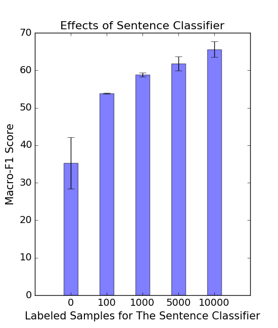
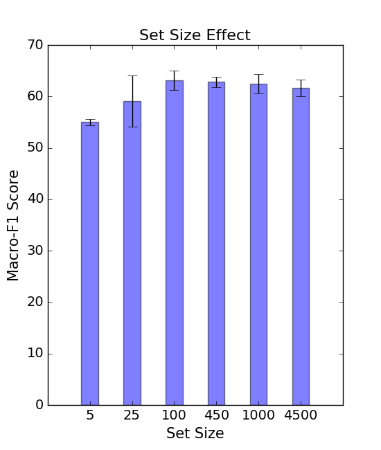
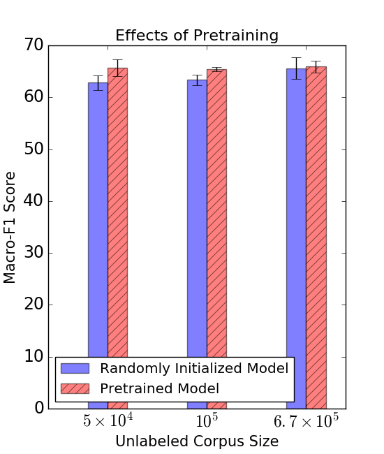
(a)	(b)	(c)	(d)

Figure 3: Macro-F1 scores for the entire SemEval-2016 dataset of the different analyses. (a) the contribution of unlabeled data. (b) the effect of sentence classifier quality. (c) the effect of k. (d) the effect of sentence-level pretraining vs. corpus size.

Data	Training	SemEval-15		SemEval-16
		Acc.	Macro-F1	Acc.	Macro-F1
N	BiLSTM-XR	83.31 $\pm$ 0.77	64.42 $\pm$ 2.78	88.12 $\pm$ 0.24	68.60 $\pm$ 1.79
N+A	BiLSTM-XR $\rightarrow$Aspect Based Finetuning	83.44 $\pm$ 0.74	67.23 $\pm$ 1.42	87.66 $\pm$ 0.28	71.19 $\pm$ 1.40
A	Bert$\rightarrow$Aspect Based Finetuning	81.87 $\pm$ 1.12	59.24 $\pm$ 4.94	85.81 $\pm$ 1.07	62.46 $\pm$ 6.76
S	Bert$\rightarrow$$10^{4}$ Sent Finetuning	83.29 $\pm$ 0.77	66.79 $\pm$ 1.99	84.53 $\pm$ 1.66	65.53 $\pm$ 3.03
S+A	Bert$\rightarrow$$10^{4}$ Sent Finetuning $\rightarrow$Aspect Based Finetuning	82.54 $\pm$ 1.21	64.13 $\pm$ 5.05	85.67 $\pm$ 1.14	64.13 $\pm$ 7.07
N	Bert$\rightarrow$XR	85.46∗ $\pm$ 0.59	66.86 $\pm$ 2.8	89.5∗ $\pm$ 0.55	70.86†$\pm$ 2.96
N+A	Bert$\rightarrow$XR $\rightarrow$Aspect Based Finetuning	85.78∗ $\pm$ 0.65	68.74 $\pm$ 1.36	89.57∗ $\pm$ 1.4	73.89∗ $\pm$ 2.05

Table 2: Bert pre-training: average accuracies and Macro-F1 scores from five runs and their stdev. ^∗ indicates that the method’s result is significantly better than all baseline methods, † indicates that the method’s result is significantly better than all non XR baseline methods, with $p<0.05$ according to a one-tailed unpaired t-test. The data annotations S, N and A indicate training with Sentence-level, Noisy sentence-level and Aspect-level data respectively.

5.3 Pre-training, Bert

The XR training can be performed also over pre-trained representations. We experiment with two pre-training methods: (1) pre-training by training the BiLSTM model to predict the noisy sentence-level predictions. (2) Using the pre-trained Bert representation Devlin et al. (2018). For (1), we compare the effect of pre-train on unlabeled corpora of sizes of $5\times 10^{4}$, $10^{5}$ and $6.7\times 10^{5}$ sentences. Results in Figure 3d show that this form of pre-training is effective for smaller unlabeled corpora but evens out for larger ones.

Bert

For the Bert experiments, we experiment with the Bert-base model with $k=450$ sets, 30 epochs for XR training or sentence level fine-tuning and 15 epochs for aspect based fine-tuning, on each training method we evaluated the model on the dev set after each epoch and the best model was chosen. We compare the following setups:
-Bert$\rightarrow$Aspect Based Finetuning: pretrained bert model finetuned to the aspect based task.
-Bert$\rightarrow 10^{4}$: A pretrained bert model finetuned to the sentence level task on the $10^{4}$ sentences, and tested by predicting fragment-level sentiment.
-Bert$\rightarrow$$10^{4}$$\rightarrow$Aspect Based Finetuning: pretrained bert model finetuned to the sentence level task, and finetuned again to the aspect based one.
-Bert$\rightarrow$XR: pretrained bert model followed by XR training using our method.
-Bert$\rightarrow$ XR $\rightarrow$ Aspect Based Finetuning: pretrained bert followed by XR training and then fine-tuned to the aspect level task.

The results are presented in Table 2. As before, aspect-based fine-tuning is beneficial for both SemEval-16 and SemEval-15. Training a BiLSTM with XR surpasses pre-trained bert models and using XR training on top of the pre-trained Bert models substantially increases the results even further.

6 Discussion

We presented a transfer learning method based on expectation regularization (XR), and demonstrated its effectiveness for training aspect-based sentiment classifiers using sentence-level supervision. The method achieves state-of-the-art results for the task, and is also effective for improving on top of a strong pre-trained Bert model. The proposed method provides an additional data-efficient tool in the modeling arsenal, which can be applied on its own or together with another training method, in situations where there is a conditional relations between the labels of a source task for which we have supervision, and a target task for which we don’t.

While we demonstrated the approach on the sentiment domain, the required conditional dependence between task labels is present in many situations. Other possible application of the method includes training language identification of tweets given geo-location supervision (knowing the geographical region gives a prior on languages spoken), training predictors for renal failure from textual medical records given classifier for diabetes (there is a strong correlation between the two conditions), training a political affiliation classifier from social media tweets based on age-group classifiers, zip-code information, or social-status classifiers (there are known correlations between all of these to political affiliation), training hate-speech detection based on emotion detection, and so on.

References

- Byrd et al. (1995) Richard H. Byrd, Peihuang Lu, Jorge Nocedal, and Ciyou Zhu. 1995. A limited memory algorithm for bound constrained optimization. SIAM J. Scientific Computing, 16(5):1190–1208.
- Chang et al. (2007) Ming-Wei Chang, Lev Ratinov, and Dan Roth. 2007. Guiding semi-supervision with constraint-driven learning. In Proceedings of the 45th Annual Meeting of the Association of Computational Linguistics, pages 280–287. Association for Computational Linguistics.
- Chang et al. (2012) Ming-Wei Chang, Lev-Arie Ratinov, and Dan Roth. 2012. Structured learning with constrained conditional models. Machine Learning, 88(3):399–431.
- Chen et al. (2017) Peng Chen, Zhongqian Sun, Lidong Bing, and Wei Yang. 2017. Recurrent attention network on memory for aspect sentiment analysis. In Proceedings of the 2017 Conference on Empirical Methods in Natural Language Processing, pages 452–461. Association for Computational Linguistics.
- Devlin et al. (2018) Jacob Devlin, Ming-Wei Chang, Kenton Lee, and Kristina Toutanova. 2018. Bert: Pre-training of deep bidirectional transformers for language understanding. CoRR, abs/1810.04805.
- Druck et al. (2008) Gregory Druck, Gideon S. Mann, and Andrew McCallum. 2008. Learning from labeled features using generalized expectation criteria. In Proceedings of the 31st Annual International ACM SIGIR Conference on Research and Development in Information Retrieval, SIGIR 2008, Singapore, July 20-24, 2008, pages 595–602.
- Fan et al. (2018a) Chuang Fan, Qinghong Gao, Jiachen Du, Lin Gui, Ruifeng Xu, and Kam-Fai Wong. 2018a. Convolution-based memory network for aspect-based sentiment analysis. In The 41st International ACM SIGIR Conference on Research & Development in Information Retrieval, SIGIR 2018, Ann Arbor, MI, USA, July 08-12, 2018, pages 1161–1164.
- Fan et al. (2018b) Feifan Fan, Yansong Feng, and Dongyan Zhao. 2018b. Multi-grained attention network for aspect-level sentiment classification. In Proceedings of the 2018 Conference on Empirical Methods in Natural Language Processing, pages 3433–3442. Association for Computational Linguistics.
- Ganchev and Das (2013) Kuzman Ganchev and Dipanjan Das. 2013. Cross-lingual discriminative learning of sequence models with posterior regularization. In Proceedings of the 2013 Conference on Empirical Methods in Natural Language Processing, pages 1996–2006. Association for Computational Linguistics.
- Ganchev et al. (2010) Kuzman Ganchev, João Graça, Jennifer Gillenwater, and Ben Taskar. 2010. Posterior regularization for structured latent variable models. Journal of Machine Learning Research, 11:2001–2049.
- Graça et al. (2007) João Graça, Kuzman Ganchev, and Ben Taskar. 2007. Expectation maximization and posterior constraints. In Advances in Neural Information Processing Systems 20, Proceedings of the Twenty-First Annual Conference on Neural Information Processing Systems, Vancouver, British Columbia, Canada, December 3-6, 2007, pages 569–576.
- Haghighi and Klein (2006) Aria Haghighi and Dan Klein. 2006. Prototype-driven learning for sequence models. In Human Language Technology Conference of the North American Chapter of the Association of Computational Linguistics, Proceedings, June 4-9, 2006, New York, New York, USA.
- He et al. (2018a) Ruidan He, Wee Sun Lee, Hwee Tou Ng, and Daniel Dahlmeier. 2018a. Effective attention modeling for aspect-level sentiment classification. In Proceedings of the 27th International Conference on Computational Linguistics, pages 1121–1131. Association for Computational Linguistics.
- He et al. (2018b) Ruidan He, Wee Sun Lee, Hwee Tou Ng, and Daniel Dahlmeier. 2018b. Exploiting document knowledge for aspect-level sentiment classification. In Proceedings of the 56th Annual Meeting of the Association for Computational Linguistics (Volume 2: Short Papers), pages 579–585. Association for Computational Linguistics.
- Hinton et al. (2012) Geoffrey E. Hinton, Nitish Srivastava, Alex Krizhevsky, Ilya Sutskever, and Ruslan Salakhutdinov. 2012. Improving neural networks by preventing co-adaptation of feature detectors. CoRR, abs/1207.0580.
- Hope and Shahaf (2016) Tom Hope and Dafna Shahaf. 2016. Ballpark learning: Estimating labels from rough group comparisons. In Machine Learning and Knowledge Discovery in Databases - European Conference, ECML PKDD 2016, Riva del Garda, Italy, September 19-23, 2016, Proceedings, Part II, pages 299–314.
- Jin and Liu (2005) Rong Jin and Yi Liu. 2005. A framework for incorporating class priors into discriminative classification. In Advances in Knowledge Discovery and Data Mining, 9th Pacific-Asia Conference, PAKDD 2005, Hanoi, Vietnam, May 18-20, 2005, Proceedings, pages 568–577.
- Kingma and Ba (2014) Diederik P. Kingma and Jimmy Ba. 2014. Adam: A method for stochastic optimization. CoRR, abs/1412.6980.
- Li et al. (2018) Lishuang Li, Yang Liu, and AnQiao Zhou. 2018. Hierarchical attention based position-aware network for aspect-level sentiment analysis. In Proceedings of the 22nd Conference on Computational Natural Language Learning, pages 181–189. Association for Computational Linguistics.
- Liang et al. (2009) Percy Liang, Michael I. Jordan, and Dan Klein. 2009. Learning from measurements in exponential families. In Proceedings of the 26th Annual International Conference on Machine Learning, ICML 2009, Montreal, Quebec, Canada, June 14-18, 2009, pages 641–648.
- Liu et al. (2018) Fei Liu, Trevor Cohn, and Timothy Baldwin. 2018. Recurrent entity networks with delayed memory update for targeted aspect-based sentiment analysis. In Proceedings of the 2018 Conference of the North American Chapter of the Association for Computational Linguistics: Human Language Technologies, Volume 2 (Short Papers), pages 278–283. Association for Computational Linguistics.
- Liu and Zhang (2017) Jiangming Liu and Yue Zhang. 2017. Attention modeling for targeted sentiment. In Proceedings of the 15th Conference of the European Chapter of the Association for Computational Linguistics: Volume 2, Short Papers, pages 572–577. Association for Computational Linguistics.
- Ma et al. (2017) Dehong Ma, Sujian Li, Xiaodong Zhang, and Houfeng Wang. 2017. Interactive attention networks for aspect-level sentiment classification. In Proceedings of the Twenty-Sixth International Joint Conference on Artificial Intelligence, IJCAI 2017, Melbourne, Australia, August 19-25, 2017, pages 4068–4074.
- Mann and McCallum (2007) Gideon S. Mann and Andrew McCallum. 2007. Simple, robust, scalable semi-supervised learning via expectation regularization. In Machine Learning, Proceedings of the Twenty-Fourth International Conference (ICML 2007), Corvallis, Oregon, USA, June 20-24, 2007, pages 593–600.
- Mann and McCallum (2010a) Gideon S. Mann and Andrew McCallum. 2010a. Generalized expectation criteria for semi-supervised learning with weakly labeled data. Journal of Machine Learning Research, 11:955–984.
- Mann and McCallum (2010b) Gideon S. Mann and Andrew McCallum. 2010b. Generalized expectation criteria for semi-supervised learning with weakly labeled data. Journal of Machine Learning Research, 11:955–984.
- Melville et al. (2009) Prem Melville, Wojciech Gryc, and Richard D. Lawrence. 2009. Sentiment analysis of blogs by combining lexical knowledge with text classification. In Proceedings of the 15th ACM SIGKDD International Conference on Knowledge Discovery and Data Mining, Paris, France, June 28 - July 1, 2009, pages 1275–1284.
- Mohammady and Culotta (2015) Ardehaly Ehsan Mohammady and Aron Culotta. 2015. Inferring latent attributes of twitter users with label regularization. In Proceedings of the 2015 Conference of the North American Chapter of the Association for Computational Linguistics: Human Language Technologies, pages 185–195. Association for Computational Linguistics.
- Musicant et al. (2007) David R. Musicant, Janara M. Christensen, and Jamie F. Olson. 2007. Supervised learning by training on aggregate outputs. In Proceedings of the 7th IEEE International Conference on Data Mining (ICDM 2007), October 28-31, 2007, Omaha, Nebraska, USA, pages 252–261.
- Neubig et al. (2017) Graham Neubig, Chris Dyer, Yoav Goldberg, Austin Matthews, Waleed Ammar, Antonios Anastasopoulos, Miguel Ballesteros, David Chiang, Daniel Clothiaux, Trevor Cohn, Kevin Duh, Manaal Faruqui, Cynthia Gan, Dan Garrette, Yangfeng Ji, Lingpeng Kong, Adhiguna Kuncoro, Gaurav Kumar, Chaitanya Malaviya, Paul Michel, Yusuke Oda, Matthew Richardson, Naomi Saphra, Swabha Swayamdipta, and Pengcheng Yin. 2017. Dynet: The dynamic neural network toolkit. CoRR, abs/1701.03980.
- Nguyen and Shirai (2015) Thien Hai Nguyen and Kiyoaki Shirai. 2015. Phrasernn: Phrase recursive neural network for aspect-based sentiment analysis. In Proceedings of the 2015 Conference on Empirical Methods in Natural Language Processing, pages 2509–2514. Association for Computational Linguistics.
- Ouyang and Su (2018) Zhifan Ouyang and Jindian Su. 2018. Dependency parsing and attention network for aspect-level sentiment classification. In Natural Language Processing and Chinese Computing - 7th CCF International Conference, NLPCC 2018, Hohhot, China, August 26-30, 2018, Proceedings, Part I, pages 391–403.
- Pennington et al. (2014) Jeffrey Pennington, Richard Socher, and Christopher Manning. 2014. Glove: Global vectors for word representation. In Proceedings of the 2014 Conference on Empirical Methods in Natural Language Processing (EMNLP), pages 1532–1543. Association for Computational Linguistics.
- Pontiki et al. (2016) Maria Pontiki, Dimitris Galanis, Haris Papageorgiou, Ion Androutsopoulos, Suresh Manandhar, Mohammad AL-Smadi, Mahmoud Al-Ayyoub, Yanyan Zhao, Bing Qin, Orphee De Clercq, Veronique Hoste, Marianna Apidianaki, Xavier Tannier, Natalia Loukachevitch, Evgeniy Kotelnikov, Núria Bel, Salud María Jiménez-Zafra, and Gülşen Eryiğit. 2016. Semeval-2016 task 5: Aspect based sentiment analysis. In Proceedings of the 10th International Workshop on Semantic Evaluation (SemEval-2016), pages 19–30. Association for Computational Linguistics.
- Pontiki et al. (2015) Maria Pontiki, Dimitris Galanis, Haris Papageorgiou, Suresh Manandhar, and Ion Androutsopoulos. 2015. Semeval-2015 task 12: Aspect based sentiment analysis. In Proceedings of the 9th International Workshop on Semantic Evaluation (SemEval 2015), pages 486–495. Association for Computational Linguistics.
- Quadrianto et al. (2009a) Novi Quadrianto, Alexander J. Smola, Tibério S. Caetano, and Quoc V. Le. 2009a. Estimating labels from label proportions. Journal of Machine Learning Research, 10:2349–2374.
- Quadrianto et al. (2009b) Novi Quadrianto, Alexander J. Smola, Tibério S. Caetano, and Quoc V. Le. 2009b. Estimating labels from label proportions. Journal of Machine Learning Research, 10:2349–2374.
- Ruder et al. (2016) Sebastian Ruder, Parsa Ghaffari, and John G. Breslin. 2016. A hierarchical model of reviews for aspect-based sentiment analysis. In Proceedings of the 2016 Conference on Empirical Methods in Natural Language Processing, pages 999–1005. Association for Computational Linguistics.
- Schapire et al. (2002) Robert E. Schapire, Marie Rochery, Mazin G. Rahim, and Narendra K. Gupta. 2002. Incorporating prior knowledge into boosting. In Machine Learning, Proceedings of the Nineteenth International Conference (ICML 2002), University of New South Wales, Sydney, Australia, July 8-12, 2002, pages 538–545.
- Tang et al. (2016a) Duyu Tang, Bing Qin, Xiaocheng Feng, and Ting Liu. 2016a. Effective lstms for target-dependent sentiment classification. In Proceedings of COLING 2016, the 26th International Conference on Computational Linguistics: Technical Papers, pages 3298–3307. The COLING 2016 Organizing Committee.
- Tang et al. (2016b) Duyu Tang, Bing Qin, and Ting Liu. 2016b. Aspect level sentiment classification with deep memory network. In Proceedings of the 2016 Conference on Empirical Methods in Natural Language Processing, pages 214–224. Association for Computational Linguistics.
- Vo and Zhang (2015) Duy-Tin Vo and Yue Zhang. 2015. Target-dependent twitter sentiment classification with rich automatic features. In Proceedings of the Twenty-Fourth International Joint Conference on Artificial Intelligence, IJCAI 2015, Buenos Aires, Argentina, July 25-31, 2015, pages 1347–1353.
- Wang et al. (2018a) Jingjing Wang, Jie Li, Shoushan Li, Yangyang Kang, Min Zhang, Luo Si, and Guodong Zhou. 2018a. Aspect sentiment classification with both word-level and clause-level attention networks. In Proceedings of the Twenty-Seventh International Joint Conference on Artificial Intelligence, IJCAI 2018, July 13-19, 2018, Stockholm, Sweden., pages 4439–4445.
- Wang and Manning (2014) Mengqiu Wang and Christopher D. Manning. 2014. Cross-lingual projected expectation regularization for weakly supervised learning. TACL, 2:55–66.
- Wang et al. (2018b) Shuai Wang, Sahisnu Mazumder, Bing Liu, Mianwei Zhou, and Yi Chang. 2018b. Target-sensitive memory networks for aspect sentiment classification. In Proceedings of the 56th Annual Meeting of the Association for Computational Linguistics (Volume 1: Long Papers), pages 957–967. Association for Computational Linguistics.
- Wang et al. (2016) Yequan Wang, Minlie Huang, xiaoyan zhu, and Li Zhao. 2016. Attention-based lstm for aspect-level sentiment classification. In Proceedings of the 2016 Conference on Empirical Methods in Natural Language Processing, pages 606–615. Association for Computational Linguistics.
- Wang et al. (2012) Zuoguan Wang, Siwei Lyu, Gerwin Schalk, and Qiang Ji. 2012. Learning with target prior. In Advances in Neural Information Processing Systems 25: 26th Annual Conference on Neural Information Processing Systems 2012. Proceedings of a meeting held December 3-6, 2012, Lake Tahoe, Nevada, United States., pages 2240–2248.
- Yang et al. (2018) Min Yang, Qiang Qu, Xiaojun Chen, Chaoxue Guo, Ying Shen, and Kai Lei. 2018. Feature-enhanced attention network for target-dependent sentiment classification. Neurocomputing, 307:91–97.
- Zhang et al. (2016) Meishan Zhang, Yue Zhang, and Duy-Tin Vo. 2016. Gated neural networks for targeted sentiment analysis. In Proceedings of the Thirtieth AAAI Conference on Artificial Intelligence, February 12-17, 2016, Phoenix, Arizona, USA., pages 3087–3093.
- Zhu et al. (2014) Jun Zhu, Ning Chen, and Eric P. Xing. 2014. Bayesian inference with posterior regularization and applications to infinite latent svms. Journal of Machine Learning Research, 15(1):1799–1847.