Stochastic Convolutional Sparse Coding

Abstract

State-of-the-art methods for Convolutional Sparse Coding usually employ Fourier-domain solvers in order to speed up the convolution operators. However, this approach is not without shortcomings. For example, Fourier-domain representations implicitly assume circular boundary conditions and make it hard to fully exploit the sparsity of the problem as well as the small spatial support of the filters.

In this work, we propose a novel stochastic spatial-domain solver, in which a randomized subsampling strategy is introduced during the learning sparse codes. Afterwards, we extend the proposed strategy in conjunction with online learning, scaling the CSC model up to very large sample sizes. In both cases, we show experimentally that the proposed subsampling strategy, with a reasonable selection of the subsampling rate, outperforms the state-of-the-art frequency-domain solvers in terms of execution time without losing the learning quality. Finally, we evaluate the effectiveness of the over-complete dictionary learned from large-scale datasets, which demonstrates an improved sparse representation of the natural images on account of more abundant learned image features. <ccs2012> <concept> <concept_id>10010147.10010178.10010224.10010240.10010241</concept_id> <concept_desc>Computing methodologies Image representations</concept_desc> <concept_significance>500</concept_significance> </concept> <concept> <concept_id>10003752.10003809.10010047.10010048</concept_id> <concept_desc>Theory of computation Online learning algorithms</concept_desc> <concept_significance>100</concept_significance> </concept> </ccs2012>

[500]Computing methodologies Image representations [100]Theory of computation Online learning algorithms

1 Introduction

Convolutional Sparse Coding (CSC) is a method for learning generative models in the form of translationally invariant dictionaries for a large variety of different training signals. These generative models have been shown effective for solving problems in neural and brain information processing [JLTSG17, PKB^∗17], as well as in a variety of image processing tasks, for instance, image inpainting [HHW15], super-resolution [GZX^∗15], high dynamic range imaging [SHG^∗16], and high-dimensional signal reconstructions [CSH^∗17, BG17]. CSC differs from conventional sparse coding by formulating the signals as the sum of a set of convolutions on dictionary filters and sparse codes instead of patch-wise linear combinations of filters. In traditional sparse dictionary learning, the patch structure significantly degrades the expressiveness of the dictionaries by introducing a strong dependency on the position of a feature, which the convolutional nature of CSC avoids.

This convolutional approach is also at the heart of many deep learning-based methods in the form of CNNs [LBBH98, KSB^∗10, KSH12], which have in recent years been extraordinarily successful for a broad range of high-level image understanding applications. However, while CNNs generally are used in a supervised setting and produce discriminative, task-specific models, CSC is unsupervised and produces generative models that can easily be transferred between tasks.

To solve the optimization problems inherent to CSC, Zeiler et al. [ZKTF10] iteratively solve two subproblems (updating sparse codes and updating filters) using gradient decent in the form of convolutional operations in the spatial domain, which is computationally expensive. Recent algorithms tackle the problem by exploiting Parseval’s theorem to express the spatial convolution by multiplication in the frequency domain and using proximal solver such as Alternating Direction Method of Multipliers (ADMM) [BPC^∗11] to separate the linear least squares parts from the non-smooth terms in the optimization problem. These approaches show tremendous improvements over prior spatial-domain solvers with respect to running time [BEL13, HHW15, Woh16, CSH^∗17]. Most of the prior work learns the dictionary filters in a batch mode, which indicates that all training signals are involved in every training iteration, and this restricts it from applying to large datasets or streaming data.

In contrast to batch mode learning, online learning [SS^∗12] is a well established strategy which processes a single image or a small portion (mini-batch) of the whole data at each training step, and incrementally updates model variables. Herein, the required memory and computing sources are only dependent on the sample size in every observation, independent of the training data size. It alleviates the scalability issue that arises in batch approaches, and the convergence of the algorithm was firstly analyzed using stochastic approximation tools [Bot98]. Bottou et al. [BB08] further showed better generalization performance of the stochastic algorithms than standard gradient descent on large scale learning systems. Later on, online learning strategies were synergetic with sparse coding, which was then scaled up for learning dictionary from millions of training samples [MBPS09, MBPS10], and for large-scale matrix factorization with an additionally introduced subsampling strategy [MMTV16]. More recently, Liu et al. [LGCWY18] and Wang et al. [WYKN18] separately proposed similar online learning frameworks for the CSC model, alleviating the memory issues arise in batch-based CSC model on large datasets.

Contributions. We mainly make three contributions in this work. First, we introduce a randomization strategy for the CSC model and solve the entire problems in the spatial domain. We demonstrate that the proposed stochastic spatial-domain solver, with a reasonably selected subsampling rate, outperforms the state-of-the-art frequency-domain solvers with regard to computing efficiency. Secondly, we formulate an online-learning version of the proposed algorithm, and show dramatic runtime improvement over current online CSC methods, while producing comparable outcomes. Finally, we demonstrate the capability to learn the meaningful over-complete dictionary from thousands of images, and analyze the effectiveness of the learned over-complete dictionary for a number of reconstruction tasks.

2 Convolutional Sparse Coding (CSC)

The dictionary learning problem for CSC problem has the form

$$\begin{split}\underset{{{\mathbf{d}},{\mathbf{z}}}}{\operatorname{min}}\>\>&\frac{1}{2}\|{\mathbf{x}}-\sum_{\mathrm{k=1}}^{K}{\mathbf{d}}_{\mathrm{k}}*{\mathbf{z}}_{\mathrm{k}}\|_{\mathrm{2}}^{2}+\lambda\sum_{\mathrm{k=1}}^{K}\|{\mathbf{z}}_{\mathrm{k}}\|_{\mathrm{1}}\\ \text{subject to}&~{}\|{\mathbf{d}}_{\mathrm{k}}\|^{2}_{\mathrm{2}}\leq 1~{}~{}\forall k\in\{1,\dots,K\},\end{split}$$ (1)

where ${\mathbf{x}}\in\mathbb{R}^{D}$ is a $D$-dimensional signal or a vectorized image, ${\mathbf{d}}_{\mathrm{k}}\in\mathbb{R}^{M}$ is the $k$-th dictionary, ${\mathbf{z}}_{\mathrm{k}}\in\mathbb{R}^{D}$ is the sparse code associated with that dictionary, $\lambda>0$ is a sparsity inducing penalty parameter, $K$ is the number of dictionary filters, and $*$ is the convolution operator. The above model will be applied to all the training images ${\mathbf{x}}\in\mathbb{X}$.

Most recent CSC algorithms exploit Parseval’s theorem and introduce two slack variables to separate the non-smooth $L_{\mathrm{1}}$ penalty term and the $L_{\mathrm{2}}$ constraints, making it feasible to efficiently compute the latter in the frequency domain. Furthermore, the whole Problem (1) can be split into alternating subproblems for updating ${\mathbf{z}}$ and ${\mathbf{d}}$, which are jointly solved by coordinate descent [BEL13, HHW15, Woh16]. This approach suffers from several issues:

• While CSC overcomes the independence assumption held in patch-based learning algorithms, far more variables ($K$ times more) are introduced to represent a single image to compensate for this. This creates more severe memory and computational burdens.

• We observe through experiments that the vast majority of the entries of the reconstructed sparse codes do not provide useful information about the represented image. For $K=100$, 99.5% entries are not informative. This indicates that the subproblem for updating ${\mathbf{z}}$ solves a highly sparse LASSO problem. Transforming the problem into frequency domain imposes restrictions on exploiting this sparsity.

• While prior work shows its efficiency in solving the CSC problem in the frequency domain, this is only applicable for updating ${\mathbf{z}}$, and does not hold for updating ${\mathbf{d}}$. The dictionary filters usually have much smaller spatial support than the dimension size of the sparse codes ($M\ll D$). However, in order to tackle the problem in the frequency domain, it is necessary to process the ${\mathbf{d}}$-subproblem over the full support of the sparse codes, and then project the results onto the much smaller spatial support of the filters.

3 Stochastic Convolutional Sparse Coding

3.1 The SCSC Model

We first define a stacked vector ${\mathbf{z}}=[{\mathbf{z}}_{\mathrm{1}},\dots,{\mathbf{z}}_{\mathrm{K}}]\in\mathbb{R}^{DK}$ for the codes, as well as a stacked matrix ${\mathbf{D}}=[{\mathbf{D}}_{\mathrm{1}},\dots,{\mathbf{D}}_{\mathrm{K}}]\in\mathbb{R}^{D\times DK}$ for the filter convolutions. The convolution operators are expressed as a matrix multiplication so that ${\mathbf{D}}{\mathbf{z}}=\sum_{\mathrm{k=1}}^{K}{\mathbf{d}}_{\mathrm{k}}*{\mathbf{z}}_{\mathrm{k}}$. Therefore, each part of ${\mathbf{D}}$ is a Toeplitz matrix.

Based on the strong sparsity of the codes ${\mathbf{z}}$, we propose to implement the CSC learning problem (1) iteratively, where at the $t$-th iteration we only consider a random subset of the codes, denoted as $\tilde{{\mathbf{z}}}^{t}\in\mathbb{R}^{pDK}$. We subsample the sparse codes ${\mathbf{z}}$ following a Bernoulli distribution with probability $p$. This subsampling process can be expressed as a matrix operation

$$\tilde{{\mathbf{z}}}^{t}={\mathbf{M}}^{t}{\mathbf{z}}^{t},$$ (2)

where ${\mathbf{M}}^{t}$ is a $\mathbb{R}^{pDk\times DK}$ binary matrix, where exactly one entry per row has a value of $1$, and the other entries are $0$. For each iteration $t$, a different matrix ${\mathbf{M}}^{t}$ is generated randomly. This matrix projects the codes ${\mathbf{z}}^{t}$ to a random subspace, retaining the sampled codes and filtering out the others. In the case of $p=1$, the proposed model is identical to the classical CSC model, and ${\mathbf{M}}$ is simply an identity matrix. When $p<1$, the algorithm only solves a subset of the codes at chosen positions in each iteration, and accordingly, the update of dictionary ${\mathbf{d}}$ is based on the selected portion of the codes $\tilde{{\mathbf{z}}}$. Similar to solving the classical CSC problem, we can apply a coordinate descent algorithm, alternating on subproblems of $\tilde{{\mathbf{z}}}$ and ${\mathbf{d}}$, to tackle the bi-convex optimization problem. Specifically, the modified minimization problem for $\tilde{{\mathbf{z}}}$ can be formulated as:

$$\tilde{{\mathbf{z}}}^{t}=\underset{{\tilde{{\mathbf{z}}}}}{\operatorname{argmin}}\>\>\frac{1}{2}\|{\mathbf{x}}-{\mathbf{D}}^{t-1}({\mathbf{M}}^{t})^{\top}\tilde{{\mathbf{z}}}\|_{\mathrm{2}}^{2}+\lambda\|\tilde{{\mathbf{z}}}\|_{\mathrm{1}},$$ (3)

where ${\mathbf{D}}^{t-1}$ is composed of the dictionary learned in the $(t-1)$-th iteration. Due to the introduced subsampling matrix, the convolution operator cannot be implemented in the Fourier domain. However, owing to the subsampling strategy, the number of variables that need to be computed for this subproblem is $pDK$ instead of $DK$, which leads to a reduction of the spatial-domain computation time by a factor of $\frac{1}{p}$.

After computing the subsampled codes $\tilde{{\mathbf{z}}}^{t}$, we can then project them onto the original spatial support by

$${\mathbf{z}}^{t}=({\mathbf{M}}^{t})^{\top}\tilde{{\mathbf{z}}}^{t}.$$ (4)

Afterwards, the dictionary can be updated by solving the optimization problem

$$\begin{split}&{\mathbf{d}}^{t}=\underset{{{\mathbf{d}}}}{\operatorname{argmin}}\>\>\frac{1}{2}\|{\mathbf{x}}-{\mathbf{Z}}^{t}{\mathbf{d}}\|_{\mathrm{2}}^{2}\\ &\text{subject to}~{}\|{\mathbf{d}}_{\mathrm{k}}\|^{2}_{\mathrm{2}}\leq 1~{}\forall k\in\{1,\dots,K\},\end{split}$$ (5)

where ${\mathbf{Z}}^{t}=[{\mathbf{Z}}_{\mathrm{1}}^{t},\dots,{\mathbf{Z}}_{\mathrm{K}}^{t}]\in\mathbb{R}^{D\times MK}$ is a concatenation of Toeplitz matrices, and ${\mathbf{Z}}_{\mathrm{k}}^{t}$ is constructed from the associated ${\mathbf{z}}_{\mathrm{k}}^{t}$, ${\mathbf{d}}=[{\mathbf{d}}_{\mathrm{1}},\dots,{\mathbf{d}}_{\mathrm{K}}]\in\mathbb{R}^{MK}$ such that ${\mathbf{Z}}{\mathbf{d}}=\sum_{\mathrm{k=1}}^{K}{\mathbf{d}}_{\mathrm{k}}*{\mathbf{z}}_{\mathrm{k}}$. In typical CSC settings, $M\ll D$, hence there is no need to perform subsampling on the dictionary. Notice that the time complexity of solving the ${\mathbf{d}}$-update step in spatial domain is dependent of $M$, in contrast with that of frequency-domain solvers, which is $D$ dependent. This addresses the third issue in Section 2.

Our proposed randomization approach utilizes ideas similar to the stochastic Frank-Wolfe algorithm [RSPS16, KPd18]. The general idea is to solve the optimization problem on a subset of the variables at each iteration, which are randomly extracted based on a certain probability distribution. For the proposed algorithm, each iteration extracts ($pDK+MK$) variables, where $pDK$ variables are randomly picked from a total $DK$ variables, and the rest remain unchanged. Owing to the fact that CSC model is over-parameterized and the codes are highly sparse, the original signals can still be represented by a portion of the codes under a reasonable subsampling rate. Therefore, the convergence of the proposed algorithm will not be significantly affected by the subsampling manipulation, unlike the general case of the stochastic Frank-Wolfe algorithm, which usually requires more iterations to reach convergence. This insight is experimentally verified in Section 4.

In the following we introduce two different outer loop structures to utilize the proposed subsampling strategy. First, we introduce a batch mode method (stochastic batch CSC) that learns from all images simultaneously, and second we introduce an online variant (stochastic online CSC).

3.2 Stochastic Batch CSC (SBCSC)

We first introduce a batch-mode version of the proposed method as shown in Algorithm 1, where $N$ is the number of total input images, $(\tilde{{\mathbf{z}}}^{i})^{t}$ is the sampled codes associated with $i$-th image at $t$-th iteration and $({\mathbf{z}}^{i})^{t}$ is the corresponding codes in the original spatial support, $p$ is the uniform probability for one code been selected. We choose $p=\{1,0.5,0.2,0.1,0.05\}$ for testing in this work, where $p=1$ indicates no subsampling, and $p=0.05$ indicates a subsampling rate of $5\%$.

Algorithm 1 SBCSC

1:$\text{Initialize}~{}t=0,~{}{\mathbf{d}}^{t},~{}p$

2:while not converge do

3:     $t\leftarrow t+1$

4:     $\text{Randomly sample }{\mathbf{z}}^{t}\text{ with rate }p$

5:     for i=1 to N do

6:         $\text{Compute }(\tilde{{\mathbf{z}}}^{i})^{t}\text{ by solving problem~{}(\ref{eq:updatingCode}})$

7:         $\text{Compute }({\mathbf{z}}^{i})^{t}\text{ by Eq.~{}\ref{eq:upsampleCode}}$

8:     end for

9:     $\text{Compute }{\mathbf{d}}^{t}\text{ by solving problem~{}(\ref{eq:updatingFilter}})$

10:end while

Problem (3) is the standard LASSO, which can be solved by plenty of optimization frameworks. We found that solving it with ADMM delivers a good balance between computation time and convergence within a moderate number of iterations. Specifically, the data fitting term and the $L_{\mathrm{1}}$ penalty term are split, forming two separate substeps. The first substep is a quadratic programming (QP) problem, and we can either cache the matrix factorization by Cholesky decomposition (when $N$ is relatively large), or solve it iteratively by Conjugate Gradient (when $N$ is relatively small). The second substep can be solved by a point-wise shrinkage operation. Problem (5) is a quadratic constrained quadratic programming (QCQP) problem, and it can be efficiently solved by projected block coordinate decent. Empirically, a single iteration is enough with ${\mathbf{d}}$ computed in previous iteration as a warm start. We set the hyper-parameters $\lambda=1$, the ADMM iteration fixed to 10, the augmented Lagrangian penalty $\rho$ to $10\lambda$, and the over-relaxation strategy within ADMM is applied with $\alpha=1.8$. For a detailed description of the above two solvers, please refer to the supplement.

Every outer loop of SBCSC involves all of the training images, which makes it computationally expensive to process them all simultaneously. Furthermore, memory consumption quickly becomes an issue with increasing numbers of images. Thus, the batch-based learning algorithm lacks the ability to scale up to very large datasets or to handle dynamically changing training data.

3.3 Stochastic Online CSC (SOCSC)

Algorithm 2 SOCSC

1:$\text{Initialize}~{}t=0,~{}{\mathbf{d}}^{t},~{}p,~{}{\mathbf{C}}^{t}=0,~{}{\mathbf{B}}^{t}=0$

2:while not converge do

3:     $t\leftarrow t+1$

4:     $\text{draw }{\mathbf{x}}^{t}\text{ from training images}$

5:     $\text{Randomly sample }{\mathbf{z}}^{t}\text{ with rate }p$

6:     $\text{Compute }\tilde{{\mathbf{z}}}^{t}\text{ by solving problem~{}(\ref{eq:updatingCodeOnline}) using }{\mathbf{d}}^{t-1}$

7:     Compute ${\mathbf{z}}^{t}$ by Eq. 4

8:     Compute ${\mathbf{C}}^{t}$ and ${\mathbf{B}}^{t}$ by Eq. 8

9:     Compute ${\mathbf{d}}^{t}$ by solving problem (9)

10:end while

In order to address this scalability issue, we can tackle the Stochastic CSC problem in an online fashion. In the online learning setting as shown in Algorithm 2, each iteration only draws one or a subset (mini-batch) of the total training images, hence the complexity per loop is independent of the training sample size. Then, given the sampled image ${\mathbf{x}}^{t}$ at $t$-th iteration, we can compute the corresponding subsampled sparse codes $\tilde{{\mathbf{z}}}^{t}$ by

$$\tilde{{\mathbf{z}}}^{t}=\underset{{\tilde{{\mathbf{z}}}}}{\operatorname{argmin}}\>\>\frac{1}{2}\|{\mathbf{x}}^{t}-{\mathbf{D}}^{t-1}({\mathbf{M}}^{t})^{\top}\tilde{{\mathbf{z}}}\|_{\mathrm{2}}^{2}+\lambda\|\tilde{{\mathbf{z}}}\|_{\mathrm{1}}.$$ (6)

The only difference between Eq.  3 is that ${\mathbf{x}}^{t}$ only contains a portion of the total images. After projecting $\tilde{{\mathbf{z}}}^{t}$ onto the original spatial support and obtaining the sparse codes ${\mathbf{z}}^{t}$, the dictionary is updated by:

$$\begin{split}&{\mathbf{d}}^{t}=\underset{{{\mathbf{d}}}}{\operatorname{argmin}}\>\>\frac{1}{2t}\sum_{\mathrm{i=1}}^{t}\|{\mathbf{x}}^{i}-{\mathbf{Z}}^{i}{\mathbf{d}}\|_{\mathrm{2}}^{2}\\ &\text{subject to}\quad\|{\mathbf{d}}_{\mathrm{k}}\|^{2}_{\mathrm{2}}\leq 1~{}\forall k\in\{1,\dots,K\}.\end{split}$$ (7)

Note that updating the dictionary in this fashion involves all of the past training images and sparse codes. Using techniques developed for regular (non-convolutional) dictionary learning [MBPS09, MBPS10], we can get rid of explicitly storing this data by introducing two surrogate matrices ${\mathbf{C}}\in\mathbb{R}^{KM\times KM}$ and ${\mathbf{B}}\in\mathbb{R}^{KM\times 1}$. These carry all of the required information for updating ${\mathbf{d}}$, and can be iteratively updated by:

$$\begin{split}{\mathbf{C}}^{t}=\frac{t-1}{t}{\mathbf{C}}^{t-1}+\frac{1}{t}({\mathbf{Z}}^{t})^{\top}{\mathbf{Z}}^{t}\\ {\mathbf{B}}^{t}=\frac{t-1}{t}{\mathbf{B}}^{t-1}+\frac{1}{t}({\mathbf{Z}}^{t})^{\top}{\mathbf{x}}^{t}\end{split}$$ (8)

With these surrogate matrices, the updated dictionary can be obtained by solving

$$\begin{split}&{\mathbf{d}}^{t}=\underset{{{\mathbf{d}}}}{\operatorname{argmin}}\>\>\frac{1}{2}{\mathbf{d}}^{\top}{\mathbf{C}}^{t}{\mathbf{d}}-{\mathbf{d}}^{\top}{\mathbf{B}}^{t}\\ &\text{subject to}\quad\|{\mathbf{d}}_{\mathrm{k}}\|_{\mathrm{2}}^{2}\leq 1~{}\forall k\in\{1,\dots,K\}.\end{split}$$ (9)

Problem (6) and problem (9) are solved in the same way as that for SBCSC.

3.4 Complexity Analysis

Recall that $D$ is the number of pixels for a single image, $K$ is the number of filters, and $M$ is the size of the filter support. Commonly, we can assume $K\approx M$. State-of-the-art frequency-domain solvers then have the time complexity $\mathcal{O}(K^{2}D+KDlog(D))$ for a single data pass.

The time complexity of updating ${\mathbf{z}}$ in our SBCSC algorithm using Conjugate Gradient is $\mathcal{O}(pKMD\sqrt{\tau})$, where $pKMD$ is the number of non-zero elements in $({\mathbf{D}}{\mathbf{M}}^{\top})$ and $\tau$ is the condition number of $({\mathbf{A}}^{\top}{\mathbf{A}}+\rho I)$ where ${\mathbf{A}}={\mathbf{D}}{\mathbf{M}}^{\top}$. With a reasonable selection of the subsampling rate, this time complexity is comparable to that of frequency-domain solvers.

Updating the filters ${\mathbf{d}}$ takes $\mathcal{O}(K^{2}M^{2})$ time. This is comparable to $\mathcal{O}(K^{2}D)$ in the common CSC setting ($M\ll D$). However, multiple ADMM iterations are required in the frequency domain to compute ${\mathbf{d}}$ while only a single pass is required by the proposed method, which greatly reduces the computation time. Overall, the proposed method has the time complexity of $\mathcal{O}(pKMD\sqrt{\tau}+K^{2}M^{2})$.

The time complexity of SOCSC for one data pass is similar to that of SBCSC, apart from two additional steps to update the surrogate matrices. Updating ${\mathbf{C}}$ and ${\mathbf{B}}$ involves computing ${\mathbf{Z}}^{\top}{\mathbf{Z}}$ and ${\mathbf{Z}}^{\top}x$. Although ${\mathbf{Z}}$ has dimensions of $D\times KM$, it is a highly sparse matrix with only $\mathcal{O}(D)$ non-zero elements. Therefore, the total performance is not affected significantly.

4 Experiments and Results

4.1 Experimental Design

We first validate the proposed algorithms on the fruit and city datasets [ZKTF10], that each consists of 10 training images of size $100\times 100$. The online-mode algorithms are then adapted to one thousand $100\times 100$ image patches randomly picked up from ImageNet [DDS^∗09]. Note that batch-based CSC commonly can only handle less than 100 images simultaneously due to the memory limitation. The dictionary size is set to $100$ filters of size $11\times 11$ pixels in all experiments except for over-complete dictionary. All training and evaluation processes in this manuscript are performed on contrast normalized images [ZKTF10, HHW15].

Figure 1: Convergence comparison between the-state-of-art method [HHW15] and the proposed method with different subsampling rate, all of which are performed on fruit dataset. Convergence is evaluated by monitoring the objective value of Eq. 1 on training images versus iterations and time, respectively.

4.2 Subsampling Strategy

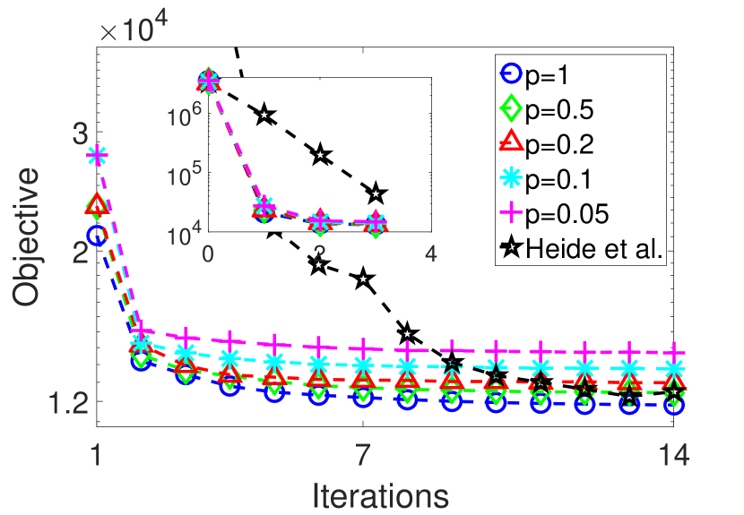
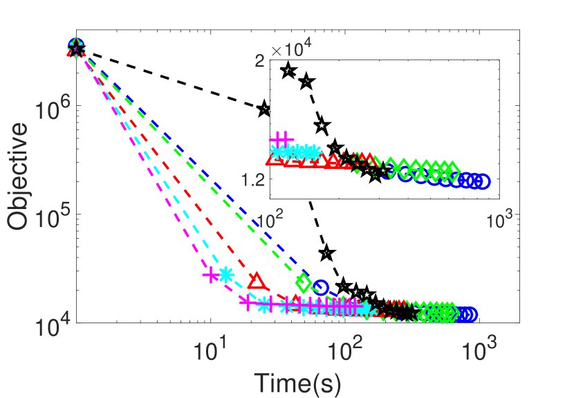
Convergence. Comparisons of the convergence between the proposed method (SBCSC) and the state-of-the-art batch-mode algorithm [HHW15] are shown in Fig. 1 (the comparison method uses a similar number of iterations as ours to reach convergence). A different selection of the subsampling rate reveals that the proposed strategy will slightly influence the convergence and the training objective of the minimization problem. Specifically, the more subsampled, the relatively slower convergence and the higher objective will be obtained. On the other hand, small subsampling rate will significantly accelerate the computation process, where $10\%$ subsampling achieves about $6\times$ speedup over the not subsampled spatial domain solver and a $2\times$ speedup over state-of-the-art Frequency-domain solver for one iteration. We observe that a subsampling rate between $p=0.1$ and $p=0.2$ delivers empirically good enough convergence in our settings, as well as achieving at least $3\times$ speedup. In general, the proposed method with various subsampling rates converges at around 10-12 iterations in all testing cases, acting similar to the competing methods.

In summary, the convergence behaviors of the proposed algorithm is only slightly influenced by the subsampling strategy within the testing subsampling rates. Comparing to the state-of-the-art frequency solver, the proposed stochastic spatial-domain solver with a subsampling rate of $0.1$ reduces the computation time by a factor of two for the tested example. Specifically, SBCSC takes 170 seconds and the comparable method takes 350 seconds for 14 iterations on a Core i7 PC. The robustness of the proposed algorithm is evaluated by additional experiments. Please see supplementary materials for reference.

4.3 Online Learning

Figure 2: The experiments are performed on fruit dataset, and each iteration randomly choose one samples from the training datasets. Top: Convergence of the test set objectives (objective value of Eq. 1 on testing datasets) for our method (SOCSC) and the current online approach [LGCWY18]. Bottom: Testing PSNR with respect to execution time. While the quality of the output is comparable, our method achieves $6\times$ speedup.

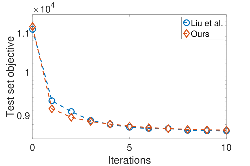
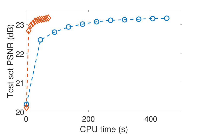
Convergence. Unlike the batch-based learning approaches which evaluate its convergence by monitoring the objective value on training datasets, a common way to evaluate the learning process of online learning model is to monitor its objective value on test datasets. In Fig. 2 we plot the objective values against the iteration number for the proposed method (SOCSC) and a recent online frequency-domain CSC method [LGCWY18] (both approaches use Matlab built-in functions only). In the same figure, we also keep track of the capability of the updated filters during the learning process to sparsely represent the test images, which is demonstrated by the time evolution of PSNR (PSNR is the peak signal-to-noise ratio, measuring the difference between the reconstructed signal and the original one). These two approaches stop at optimum positions with similar objective values. The final PSNR values for both methods also reveal a similar reconstruction performance of the learned filters. In terms of runtime comparison, however, the proposed method runs at least $6$ times faster than the comparison method. Specifically, SOCSC takes 70 seconds and the comparable method takes 440 seconds on a Core i7 PC to process all 10 training images. The supplement shows additional comparisons for the other datasets.

Figure 3: Top: number of non-zero elements in the codes for different images (on average $0.2\%$ of the variables are non-zero when $K=100$). Bottom: PSNR between the reconstructed images and the original ones with under-complete and over-complete dictionaries, respectively.

Image	1	2	3	4	5	6	7	8	9	10
PSNR by (a)	29.58	28.19	29.44	29.63	28.89	29.33	28.13	30.14	27.42	30.89
PSNR by (b)	29.63	28.22	29.57	29.90	29.12	29.59	28.05	30.17	27.53	31.08
PSNR by (c)	30.24	28.34	29.95	30.30	29.43	29.96	28.24	30.57	27.72	31.67

Figure 4: Top: Filters learned from large-scale datasets by our method (SOCSC) and the comparable online method [LGCWY18]. Bottom: $10~{}256\times 256$ testing images and their corresponding reconstruction quality in the image inpainting application. (a) The under-complete dictionary ($11\times 11\times 100$) learned by [LGCWY18]; (b) The under-complete dictionary ($11\times 11\times 100$) learned by SOCSC. (c) The over-complete dictionary ($11\times 11\times 400$) learned by SOCSC. These under-complete dictionaries, mainly composed of Gabor-like filters, can be seen as a subset of the represented over-complete dictionary, which contains a number of extra low contrast image features.

Over-complete dictionary. Learning over-complete dictionary (number of the dictionary is more than its degrees of freedom) from small datasets would cause overfitting issues, which may contain quite a few data-specific filters, and therefore limit the ability to generalize the filters to other data (we verify this explanation in the supplement). The proposed online-based learning strategy (SOCSC) can overcome this issue by scaling the model up to arbitrary sample sizes.

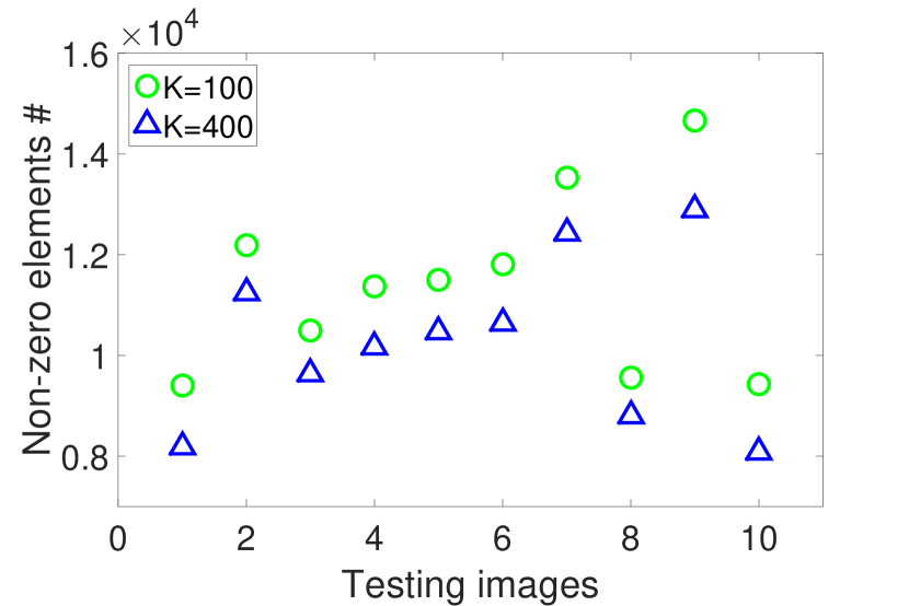
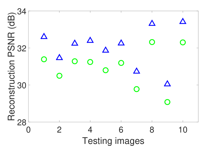
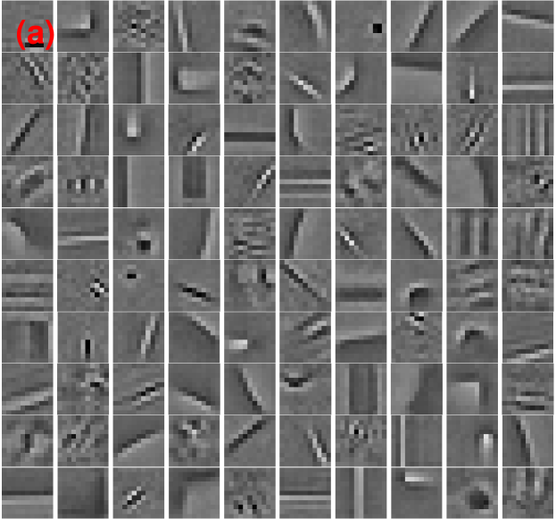
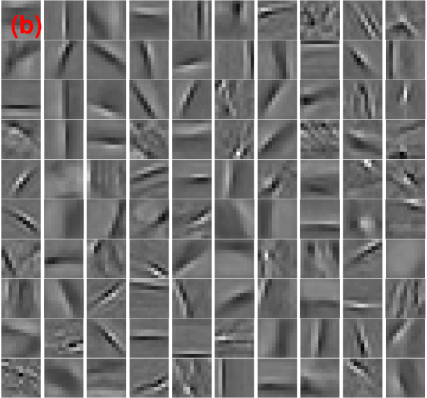
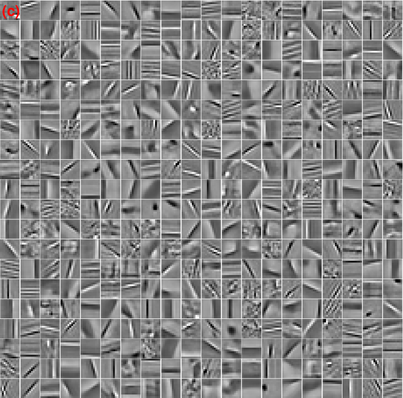
We demonstrate this ability on 1000 image patches with the size of $100\times 100$, and learn an $11\times 11\times 400$ over-complete dictionary, which is shown in Fig. 4. For a visual comparison, we also show $100$ learned filters generated by the same algorithm and another 100 filters generated by [LGCWY18]. As can be observed, both of the approaches learn visually similar under-complete dictionary, while the proposed method takes $6\times$ less training time than the comparison method. The learned over-complete dictionary is composed of the Gabor-like image features as represented in the under-complete dictionaries, as well as a number of low contrast features which are not typical for under-complete dictionaries. This additional feature information would play an essential role to reveal an improved sparse representation of the natural images. The numerical comparisons of number of non-zero elements and its corresponding reconstruction PSNR for testing images ($10~{}256\times 256$ images presented in Fig. 4) are shown in Fig. 3. Here, we define the non-zero elements as the codes whose coefficient is no less than $0.1$. We could observe that at all times, using over-complete dictionary leads to a sparser representation of the images, roughly $8\%-10\%$ reduction on the non-zero elements. Meanwhile, it achieves dramatically improved reconstruction quality, over $1$ dB on average.

We further demonstrate the effectiveness of the over-complete dictionary in the application of image inpainting, which refers to reconstructing a full image from partial measurements. A numerical comparison of the reconstruction quality is shown in the bottom of Fig. 4. The reconstructions are performed on $50\%$ randomly observed images, with $\lambda=0.4$ and $50$ ADMM iterations for all cases. Obtained PSNR values are averaged on 5 trials. The over-complete filters learned by the proposed method achieves significantly improved reconstruction quality on partially observed images in terms of the PSNR value.

We also observe a bottleneck revealed by the under-complete dictionary in the online-based CSC model. The top of Fig. 5 demonstrates that no more apparent progress could be observed when the number of training images is higher than a specific value for both of the online approaches ($K=100$). However, owing to more abundant filters, learning over-complete dictionary overcomes this bottleneck, and it shows a considerable improvement in the PSNR of image representations. All presented experimental results imply that the number of filters and number of training samples are both essential in the CSC model.

Mini-batching. In practice, a mini-batching strategy would be preferred in order to gain advantages from modern parallel computing architectures. This is also a standard extension to stochastic optimization algorithms [TBRS13, RT16, LJ17]. We denote the mini-batch size as $\eta$. In the proposed online algorithm (SOCSC), the time complexity for one step dictionary update will not increase linearly with the increase of $\eta$. Concretely speaking, updating ${\mathbf{z}}$ can be implemented by caching the Cholesky decomposition, and one computation of the matrix factorization can be applied to all of the currently selected batches. Herein, the complexity for doing updating ${\mathbf{z}}$ $\eta$ times all together is cheaper than $\eta$ times the complexity of updating one ${\mathbf{z}}$. In addition, the time complexity for updating ${\mathbf{d}}$ is not linearly affected by the value of $\eta$, which will be executed only once in each training step regardless of $\eta$. One exception is the update of surrogate matrices which has a complexity that is linear in $\eta$. However, this step is not dominant in the runtime.

Figure 5: Top: Testing PSNR for the comparable method [LGCWY18] with $K=100$, and our method (SOCSC) with $K=100$ and $K=400$, respectively. Every iteration draws a single image from those 1000 image patches. Bottom: Testing PSNR for SOCSC ($K=400$) with varying values of $\eta$. The learned filters are examined on the test sets every $2^{i}$ iterations and also at the last iteration, where $i=0,1,\dots$. Note that all the results are generated by a single-core program.

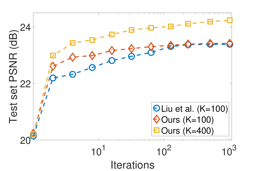
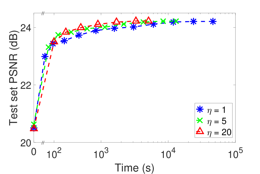
The runtime comparisons for various mini-batch sizes are shown in the bottom of Fig. 5. Note that larger $\eta$ will result in a smaller number of iterations to process all $1000$ samples. The plots show that a larger mini-batch size will generally lead to a greater progress in first few training steps, though it takes additional running time and memory. Overall, mini-batched update provides a more runtime efficient learning process in the online-based CSC model, and according to the obtained experimental results, $\eta=20$ achieves one order of magnitude speedup over $\eta=1$ to reach a a comparable level of convergence. Since computing sparse codes is a data-independent process, this mini-batched approach can be further accelerated in a distributed-computing system.

5 Conclusions

In this work, we present a novel stochastic subsampling strategy for solving the CSC problem in the spatial domain. This method exploits the sparsity of the over-parameterized model and improves the runtime performance over the prior frequency-domain solvers, which applies to both batch mode and online-learning mode. The proposed algorithm, for the first time, demonstrates the feasibility that tackling the CSC problem in spatial domain while still holding, or even improving the runtime efficiency. Since the subproblem of updating the code is a highly sparse LASSO, other specific optimization strategies can be applied to further accelerate the computation, for instance the idea proposed in [JG17], which solves the LASSO problem by coordinate descent and skips unnecessary updates using the method of safe screening [GVR12]. It is worth emphasizing that Frequency-domain methods cannot benefit from these kinds of speedup strategies.

We have also shown the capability of the developed online algorithm to learn representative and meaningful over-complete dictionary from arbitrary large datasets, and the availability of the dictionary is further verified by the application of image inpainting. It can be foreseen that this capability has widespread applications in audio and image related tasks, and higher dimensional signal processing.

6 Acknowledgements

This work was supported by King Abdullah University of Science and Technology as part of VCC center baseline funding.

References

- [BB08] Bousquet O., Bottou L.: The tradeoffs of large scale learning. In Advances in neural information processing systems (2008), pp. 161–168.
- [BEL13] Bristow H., Eriksson A., Lucey S.: Fast convolutional sparse coding. In Proceedings of the IEEE Conference on Computer Vision and Pattern Recognition (2013), pp. 391–398.
- [BG17] Bibi A., Ghanem B.: High order tensor formulation for convolutional sparse coding. In Proceedings of the IEEE Conference on Computer Vision and Pattern Recognition (2017), pp. 1772–1780.
- [Bot98] Bottou L.: Online learning and stochastic approximations. On-line learning in neural networks 17, 9 (1998), 142.
- [BPC∗11] Boyd S., Parikh N., Chu E., Peleato B., Eckstein J., et al.: Distributed optimization and statistical learning via the alternating direction method of multipliers. Foundations and Trends® in Machine learning 3, 1 (2011), 1–122.
- [CSH∗17] Choudhury B., Swanson R., Heide F., Wetzstein G., Heidrich W.: Consensus convolutional sparse coding. In Proceedings of the IEEE International Conference on Computer Vision (2017), pp. 4290–4298.
- [DDS∗09] Deng J., Dong W., Socher R., Li L.-J., Li K., Fei-Fei L.: Imagenet: A large-scale hierarchical image database. In Proceedings of the IEEE Conference on Computer Vision and Pattern Recognition (2009), pp. 248–255.
- [GVR12] Ghaoui L. E., Viallon V., Rabbani T.: Safe feature elimination for the lasso and sparse supervised learning problems. In Pacific Journal of Optimization (2012), pp. 667–698.
- [GZX∗15] Gu S., Zuo W., Xie Q., Meng D., Feng X., Zhang L.: Convolutional sparse coding for image super-resolution. In Proceedings of the IEEE International Conference on Computer Vision (2015), pp. 1823–1831.
- [HHW15] Heide F., Heidrich W., Wetzstein G.: Fast and flexible convolutional sparse coding. In Proceedings of the IEEE Conference on Computer Vision and Pattern Recognition (2015), pp. 5135–5143.
- [JG17] Johnson T. B., Guestrin C.: Stingycd: Safely avoiding wasteful updates in coordinate descent. In International Conference on Machine Learning (2017), pp. 1752–1760.
- [JLTSG17] Jas M., La Tour T. D., Simsekli U., Gramfort A.: Learning the morphology of brain signals using alpha-stable convolutional sparse coding. In Advances in Neural Information Processing Systems (2017), pp. 1099–1108.
- [KPd18] Kerdreux T., Pedregosa F., d’Aspremont A.: Frank-Wolfe with subsampling oracle. In International Conference on Machine Learning (2018), pp. 2591–2600.
- [KSB∗10] Kavukcuoglu K., Sermanet P., Boureau Y.-L., Gregor K., Mathieu M., Cun Y. L.: Learning convolutional feature hierarchies for visual recognition. In Advances in neural information processing systems (2010), pp. 1090–1098.
- [KSH12] Krizhevsky A., Sutskever I., Hinton G. E.: Imagenet classification with deep convolutional neural networks. In Advances in neural information processing systems (2012), pp. 1097–1105.
- [LBBH98] LeCun Y., Bottou L., Bengio Y., Haffner P.: Gradient-based learning applied to document recognition. Proceedings of the IEEE 86, 11 (1998), 2278–2324.
- [LGCWY18] Liu J., Garcia-Cardona C., Wohlberg B., Yin W.: First-and second-order methods for online convolutional dictionary learning. SIAM Journal on Imaging Sciences 11, 2 (2018), 1589–1628.
- [LJ17] Lei L., Jordan M. I.: Less than a single pass: Stochastically controlled stochastic gradient. In Proceedings of Machine Learning Research (AISTATS) (2017).
- [MBPS09] Mairal J., Bach F., Ponce J., Sapiro G.: Online dictionary learning for sparse coding. In International Conference on Machine Learning (2009), pp. 689–696.
- [MBPS10] Mairal J., Bach F., Ponce J., Sapiro G.: Online learning for matrix factorization and sparse coding. Journal of Machine Learning Research (2010), 19–60.
- [MMTV16] Mensch A., Mairal J., Thirion B., Varoquaux G.: Dictionary learning for massive matrix factorization. In International Conference on Machine Learning (2016), pp. 1737–1746.
- [PKB∗17] Peter S., Kirschbaum E., Both M., Campbell L., Harvey B., Heins C., Durstewitz D., Diego F., Hamprecht F. A.: Sparse convolutional coding for neuronal assembly detection. In Advances in Neural Information Processing Systems (2017), pp. 3678–3688.
- [RSPS16] Reddi S. J., Sra S., Póczos B., Smola A.: Stochastic frank-wolfe methods for nonconvex optimization. In 54th Annual Allerton Conference on Communication, Control, and Computing (Allerton) (2016), pp. 1244–1251.
- [RT16] Richtárik P., Takáč M.: Parallel coordinate descent methods for big data optimization. Mathematical Programming 156, 1-2 (2016), 433–484.
- [SHG∗16] Serrano A., Heide F., Gutierrez D., Wetzstein G., Masia B.: Convolutional sparse coding for high dynamic range imaging. In Computer Graphics Forum (2016), vol. 35, Wiley Online Library, pp. 153–163.
- [SS∗12] Shalev-Shwartz S., et al.: Online learning and online convex optimization. Foundations and Trends® in Machine Learning 4, 2 (2012), 107–194.
- [TBRS13] Takáč M., Bijral A., Richtárik P., Srebro N.: Mini-batch primal and dual methods for svms. In International Conference on Machine Learning 28 (2013), 537–552.
- [Woh16] Wohlberg B.: Efficient algorithms for convolutional sparse representations. IEEE Transactions on Image Processing 25, 1 (2016), 301–315.
- [WYKN18] Wang Y., Yao Q., Kwok J. T., Ni L. M.: Scalable online convolutional sparse coding. IEEE Transactions on Image Processing 27, 10 (2018), 4850–4859.
- [ZKTF10] Zeiler M. D., Krishnan D., Taylor G. W., Fergus R.: Deconvolutional networks. In Proceedings of the IEEE Conference on Computer Vision and Pattern Recognition (2010), pp. 2528–2535.