A Logic-Driven Framework for Consistency of Neural Models

Abstract

While neural models show remarkable accuracy on individual predictions, their internal beliefs can be inconsistent across examples. In this paper, we formalize such inconsistency as a generalization of prediction error. We propose a learning framework for constraining models using logic rules to regularize them away from inconsistency. Our framework can leverage both labeled and unlabeled examples and is directly compatible with off-the-shelf learning schemes without model redesign. We instantiate our framework on natural language inference, where experiments show that enforcing invariants stated in logic can help make the predictions of neural models both accurate and consistent.

1 Introduction

Recent NLP advances have been powered by improved representations (e.g., ELMo, BERT— Peters et al., 2018; Devlin et al., 2019), novel neural architectures (e.g., Cheng et al., 2016; Seo et al., 2017; Parikh et al., 2016; Vaswani et al., 2017), and large labeled corpora (e.g., Bowman et al., 2015; Rajpurkar et al., 2016; Williams et al., 2018). Consequently, we have seen progressively improving performances on benchmarks such as GLUE Wang et al. (2018). But, are models really becoming better? We take the position that, while tracking performance on a leaderboard is necessary to characterize model quality, it is not sufficient. Reasoning about language requires that a system has the ability not only to draw correct inferences about textual inputs, but also to be consistent its beliefs across various inputs.

To illustrate this notion of consistency, let us consider the task of natural language inference (NLI) which seeks to identify whether a premise entails, contradicts or is unrelated to a hypothesis Dagan et al. (2013). Suppose we have three sentences $P$, $H$ and $Z$, where $P$ entails $H$ and $H$ contradicts $Z$. Using these two facts, we can infer that $P$ contradicts $Z$. In other words, these three decisions are not independent of each other. Any model for textual inference should not violate this invariant defined over any three sentences, even if they are not labeled.

Neither are today’s models trained to be consistent in this fashion, nor is consistency evaluated. The decomposable attention model of Parikh et al. (2016) updated with ELMo violates the above constraint for the following sentences:

• John is on a train to Berlin.

• John is traveling to Berlin.

• John is having lunch in Berlin.

Highly accurate models can be inconsistent in their beliefs over groups of examples. For example, using a BERT-based NLI model that achieves about 90% F-score on the SNLI test set Bowman et al. (2015), we found that in about 46% of unlabeled sentence triples where $P$ entails $H$ and $H$ contradicts $Z$, the first sentence does not contradict the third. Observations of a similar spirit were also made by Minervini and Riedel (2018), Glockner et al. (2018) and Nie et al. (2018).

To characterize and eliminate such errors, first, we define a method to measure the inconsistency of models with respect to invariants stated as first-order logic formulas over model predictions. We show that our definition of inconsistency strictly generalizes the standard definition of model error.

Second, we develop a systematic framework for mitigating inconsistency in models by compiling the invariants into a differentiable loss functions using t-norms Klement et al. (2013); Gupta and Qi (1991) to soften logic. This allows us to take advantage of unlabeled examples and enforce consistency of model predictions over them. We show that the commonly used cross-entropy loss emerges as a specific instance of our framework. Our framework can be easily instantiated with modern neural network architectures.

To show the effectiveness of our approach, we instantiate it on the NLI task. We show that even state-of-the-art models can be highly inconsistent in their predictions, but our approach significantly reduces inconsistency.

In summary, our contributions are:

1. We define a mechanism to measure model inconsistency with respect to declaratively specified invariants.

2. We present a framework that compiles knowledge stated in first-order logic to loss functions that mitigate inconsistency.

3. We show that our learning framework can reduce prediction inconsistencies even with small amount of annotated examples without sacrificing predictive accuracy.

2 A Framework for (In)consistency

In this section, we will present a systematic approach for measuring and mitigating inconsistent predictions. A prediction is incorrect if it disagrees with what is known to be true. Similarly, predictions are inconsistent if they do not follow a known rule. Therefore, a model’s errors can be defined by their concordance with declarative knowledge. We will formalize this intuition by first developing a uniform representation for both labeled examples and consistency constraints (§2.1). Then, we will present a general definition of errors in the context of such a representation (§2.2). Finally, we will show a logic-driven approach for designing training losses (§ 2.3).

As a running example, we will use the NLI task whose goal is to predict one of three labels: Entailment ($E$), Contradiction ($C$), or Neutral ($N$).

2.1 Representing Knowledge

Suppose $x$ is a collection of examples (perhaps labeled). We write constraints about them as a conjunction of statements in logic:

$$\quad\bigwedge\limits_{(L,R)}L(x)\rightarrow R(x)$$ (1)

Here, $L$ and $R$ are Boolean formulas, i.e. antecedents and consequents, constructed from model predictions on examples in $x$.

One example of such an invariant is the constraint from §1, which can be written as $E(P,H)\land C(H,Z)\rightarrow C(P,Z)$, where, e.g., predicate $E(P,H)$ denotes that model predicted label $E$. We can also represent labeled examples as constraints: “If an example is annotated with label $Y^{\star}$, then model should predict so.” In logic, we write $\top\rightarrow Y^{\star}(x)$. Seen this way, the expression (1) could represent labeled data, unlabeled groups of examples with constraints between them, or a combination.

2.2 Generalizing Errors as Inconsistencies

Using the representation defined above, we can define how to evaluate predictors. We seek two properties of an evaluation metric: It should 1) quantify the inconsistency of predictions, and 2) also generalize classification error. To this end, we define two types of errors: global and conditional violation. Both are defined for a dataset $D$ consisting of example collections $x$ as described above.

Global Violation ($\boldsymbol{\rho}$)

The global violation is the fraction of examples in a dataset $D$ where any constraint is violated. We have:

$$\rho =\frac{\sum\limits_{x\in D}\left[\bigvee\limits_{(L,R)}\neg\left(L(x)\rightarrow R(x)\right)\right]}{|D|}$$ (2)

Here, $\left[\cdot\right]$ is the indicator function.

Conditional Violation ($\boldsymbol{\tau}$)

For a conditional statement, if the antecedent is not satisfied, the statement becomes trivially true. Thus, with complex antecedents, the number of examples where the constraint is true can be trivially large. To only consider those examples where the antecedent holds, we define the conditional violation as:

$$\tau =\frac{\sum\limits_{x\in D}\left[\bigvee\limits_{(L,R)}\neg\left(L(x)\rightarrow R(x)\right)\right]}{\sum\limits_{x\in D}\left[\bigvee\limits_{(L,R)}L(x)\right]}$$ (3)

Discussion

The two metrics are complementary to each other. On one hand, to lower the global metric $\rho$, a model could avoid satisfying the antecedents. In this case, the conditional metric $\tau$ is more informative. On the other hand, the global metric reflects the impact of domain knowledge in a given dataset, while the conditional one does not. Ideally, both should be low.

Both violations strictly generalize classification error. If all the knowledge we have takes the form of labeled examples, as exemplified at the end of §2.1, both violation metrics are identical to model error. The appendix formally shows this.

Name	Boolean Logic	Product	Gödel	Łukasiewicz
Negation	$\neg A$	$1-a$	$1-a$	$1-a$
T-norm	$A\wedge B$	$ab$	$\min\left(a,b\right)$	$\max\left(0,a+b-1\right)$
T-conorm	$A\vee B$	$a+b-ab$	$\max(a,b)$	$\min\left(1,a+b\right)$
Residuum	$A\rightarrow B$	$\min\left(1,\frac{b}{a}\right)$	$\begin{cases}1,\text{ if b $\geq$ a},\\ b,\text{ else}\\ \end{cases}$	$\min\left(1,1-a+b\right)$

Table 1: Mapping discrete statements to differentiable functions using t-norms. Literals are upper-cased (e.g. $A$) while real-valued probabilities are lower-cased (e.g. $a$). Here, differentiable forms are from a mixture of $R$-fuzzy logic and $S$-fuzzy logic. In this paper, we focus on the product t-norm.

2.3 Learning by Minimizing Inconsistencies

With the notion of errors, we can now focus on how to train models to minimize them. A key technical challenge involves the unification of discrete declarative constraints with the standard loss-driven learning paradigm.

To address this, we will use relaxations of logic in the form of t-norms to deterministically compile rules into differentiable loss functions. We treat predicted label probabilities as soft surrogates for Boolean decisions. In the rest of the paper, we will use lower case for model probabilities—e.g., $e(P,H)$, and upper case—e.g., $E(P,H)$—for Boolean predicates.

Different t-norms map the standard Boolean operations into different continuous functions. Table 1 summarizes this mapping for three t-norms: product, Gödel, and Łukasiewicz. Complex Boolean expressions can be constructed from these four operations. Thus, with t-norms to relax logic, we can systematically convert rules as in (1) into differentiable functions, which in turn serve as learning objectives to minimize constraint violations. We can use any off-the-shelf optimizer (e.g., ADAM Kingma and Ba, 2015). We will see concrete examples in the NLI case study in §3.

Picking a t-norm is both a design choice and an algorithmic one. Different t-norms have different numerical characteristics and their comparison is a question for future research. Here, we will focus on the product t-norm to allow comparisons to previous work: as we will see in the next section, the product t-norm strictly generalizes the widely used cross entropy loss.

3 Case Study: NLI

We study our framework using the NLI task as a case study. First, in §3.1, we will show how to represent a training set as in (1). We will also introduce two classes of domain constraints that apply to groups of premise-hypothesis pairs. Next, we will show how to compile these declaratively stated learning objectives to loss functions (§3.2). Finally, we will end this case study with a discussion about practical issues (§3.3).

3.1 Learning Objectives in Logic

Our goal is to build models that minimize inconsistency with domain knowledge stated in logic. Let us look at three such consistency requirements.

Annotation Consistency

For labeled examples, we expect that a model should predict what an annotator specifies. That is, we require

$$\forall{(P,H),Y^{\star}\in D},\quad\top\rightarrow Y^{\star}{\left(P,H\right)}$$ (4)

where $Y^{\star}$ represents the ground truth label for the example $(P,H)$. As mentioned at the end of §2.2, for the annotation consistency, both global and conditional violation rates are the same, and minimizing them is maximizing accuracy. In our experiments, we will report accuracy instead of violation rate for annotation consistency (to align with the literature).

Symmetry Consistency

Given any premise-hypothesis pair, the grounds for a model to predict Contradiction is that the events in the premise and the hypothesis cannot coexist simultaneously. That is, a $(P,H)$ pair is a contradiction if, and only if, the $(H,P)$ pair is also a contradiction:

$$\forall{(P,H)\in D},\quad C{\left(P,H\right)}\leftrightarrow C{\left(H,P\right)}$$ (5)

Transitivity Consistency

This constraint is applicable to any three related sentences $P$, $H$ and $Z$. If we group the sentences into three pairs, namely $(P,H)$, $(H,Z)$ and $(P,Z)$, the label definitions mandate that not all of the $3^{3}=27$ assignments to these three pairs are allowed. The example in §1 is an allowed label assignment. We can enumerate all such valid labels as the conjunction:

$$\begin{split}\forall{(P,H,Z)\in D},\quad\quad\quad\quad\\ \left(E\left(P,H\right)\wedge E\left(H,Z\right)\right.&\rightarrow\left.E\left(P,Z\right)\right)\\ \land\left(E\left(P,H\right)\wedge C\left(H,Z\right)\right.&\rightarrow\left.C\left(P,Z\right)\right)\\ \land\left(N\left(P,H\right)\wedge E\left(H,Z\right)\right.&\rightarrow\left.\neg C\left(P,Z\right)\right)\\ \land\left(N\left(P,H\right)\wedge C\left(H,Z\right)\right.&\rightarrow\left.\neg E\left(P,Z\right)\right)\end{split}$$ (6)

3.2 Inconsistency Losses

Using the consistency constraints stated in §3.1, we can now derive the inconsistency losses to minimize. For brevity, we will focus on the annotation and symmetry consistencies.

First, let us examine annotation consistency. We can write the universal quantifier in (4) as a conjunction to get:

$$\bigwedge\limits_{(P,H),Y^{\star}\in D}\top\rightarrow Y^{\star}{\left(P,H\right)}$$ (7)

Using the product t-norm from Table 1, we get the learning objective of maximizing the probability of the true labels:

$$\prod_{\left(P,H\right),Y^{\star}\in D}y^{\star}_{\left(P,H\right)}$$ (8)

Or equivalently, by transforming to the negative log space, we get the annotation loss:

$$L_{ann}=\sum_{\left(P,H\right),Y^{\star}\in D}-\log y^{\star}_{\left(P,H\right)}.$$ (9)

We see that we get the familiar cross-entropy loss function using the definition of inconsistency with the product t-norm!

Next, let us look at symmetry consistency:

$$\bigwedge\limits_{(P,H)\in D}C{\left(P,H\right)}\leftrightarrow C{\left(H,P\right)}.$$ (10)

Using the product t-norm, we get:

$$\prod_{\left(P,H\right)\in D}\min\left(1,\frac{c_{\left(H,P\right)}}{c_{\left(P,H\right)}}\right) \min\left(1,\frac{c_{\left(P,H\right)}}{c_{\left(H,P\right)}}\right)$$ (11)

Transforming to the negative log space as before, we get the symmetry loss:

$$L_{sym}=\sum_{\left(P,H\right)\in D}|\log c_{\left(P,H\right)}- \log c_{\left(H,P\right)}|$$ (12)

The loss for transitivity $L_{tran}$ can also be similarly derived. We refer the reader to the appendix for details.

The important point is that we can systematically convert logical statements to loss functions and cross-entropy is only one of such losses. To enforce some or all of these constraints, we add their corresponding losses. In our case study, with all constraints, the goal of learning is to minimize:

$$L =L_{ann}+\lambda_{sym}L_{sym}+\lambda_{tran}L_{tran}$$ (13)

Here, the $\lambda$’s are hyperparameters to control the influence of each loss term.

3.3 Training Constrained Models

The derived loss functions are directly compatible with off-the-shelf optimizers. The symmetry/transitivity consistencies admit using unlabeled examples, while annotation consistency requires labeled examples. Thus, in §4, we will use both labeled and unlabeled data to power training.

Ideally, we want the unlabeled dataset to be absolutely informative, meaning a model learns from every example. Unfortunately, obtaining such a dataset remains an open question since new examples are required to be both linguistically meaningful and difficult enough for the model. Minervini and Riedel (2018) used a language model to generate unlabeled adversarial examples. Another way is via pivoting through a different language, which has a long history in machine translation (e.g., Kay, 1997; Mallinson et al., 2017).

Since our focus is to study inconsistency, as an alternative, we propose a simple method to create unlabeled examples: we randomly sample sentences from the same topic. In §4, we will show that even random sentences can be surprisingly informative because the derived losses operate in real-valued space instead on discrete decisions.

	5%				100%
Config	$\rho_{{S}}$	$\tau_{{S}}$	$\rho_{{T}}$	$\tau_{{T}}$	$\rho_{{S}}$	$\tau_{{S}}$	$\rho_{{T}}$	$\tau_{{T}}$
BERT w/ SNLI	26.3	64.4	4.9	14.8	18.6	60.3	4.7	14.9
BERT w/ MultiNLI	28.4	69.3	7.0	18.5	20.6	58.9	5.6	17.5
BERT w/ SNLI+MultiNLI	25.3	62.4	4.8	14.8	18.1	59.6	4.5	14.8
BERT w/ SNLI+MultiNLI2	22.1	67.1	4.1	13.7	19.3	59.7	4.5	15.2
LSTM w/ SNLI+MultiNLI	25.8	69.5	9.9	21.0	16.8	53.6	5.3	16.0

Table 2: Inconsistencies (%) of models on our $100$k evaluation dataset. Each number represents the average of three random runs. Models are trained using $5$% and $100$% of the train sets. SNLI+MultiNLI²: finetuned twice. $\rho_{S}$ and $\tau_{S}$: symmetry consistency violations. $\rho_{T}$ and $\tau_{T}$: transitivity consistency violations.

4 Experiments

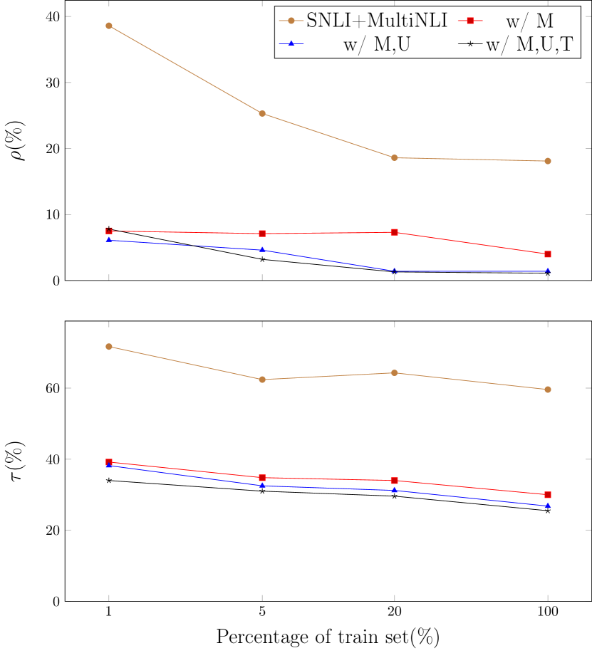
Figure 1: Symmetry inconsistencies on the $100$k evaluation example pairs. Each point represents the average of three random runs. M, U, and T are our unlabeled datasets with corresponding losses.

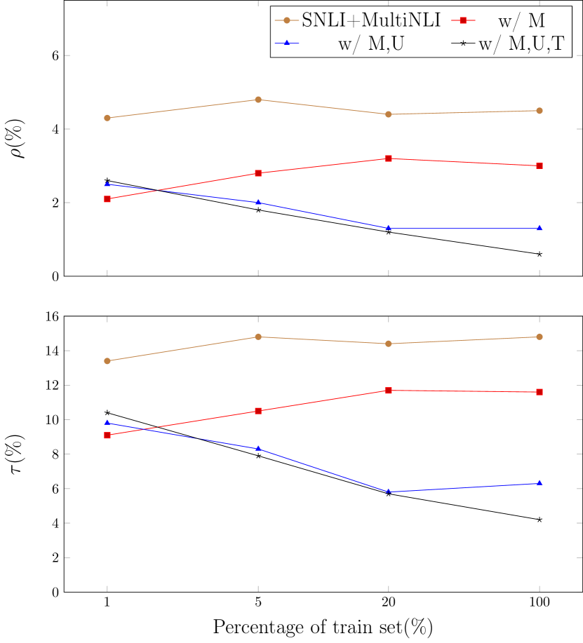
Figure 2: Transitivity inconsistencies on the $100$k evaluation example pairs. Each point represents the average of three random runs. M, U, and T are our unlabeled datasets with corresponding losses.

In this section, we evaluate our framework using (near) state-of-the-art approaches for NLI, primarily based on BERT, and also compare to an LSTM model. We use the SNLI and MultiNLI Wang et al. (2018) datasets to define annotation consistency. Our LSTM model is based on the decomposable attention model with a BiLSTM encoder and GloVe embeddings Pennington et al. (2014). Our BERT model is based on the pretrained BERT_base, finetuned on SNLI/MultiNLI. The constrained models are initialized with the finetuned BERT_base and finetuned again with inconsistency losses. For fair comparison, we also show results of BERT_base models finetuned twice.

Our constrained models are trained on both labeled and unlabeled examples. We expect that the different inconsistencies do not conflict with each other. Hence, we select hyperparameters (e.g., the $\lambda$’s) using development accuracy only (i.e., annotation consistency). We refer the reader to the appendix for details of our experimental setup.

4.1 Datasets

To be comprehensive, we will use both of the SNLI and MultiNLI to train our models, but we also show individual results.

We study the impact of the amount of label supervision by randomly sampling different percentages of labeled examples. For each case, we also sample the same percentages from the corresponding development sets for model selection. For the MultiNLI dataset, we use the matched dev for validation and mismatched dev for evaluation.

Mirrored Instances (M)

Given a labeled example, we construct its mirrored version by swapping the premise and the hypothesis. This results in the same number of unlabeled sentence pairs as the annotated dataset. When sampling by percentage, we will only use the sampled examples to construct mirrored examples. We use this dataset for symmetry consistency.

Unlabeled Instance Triples (T)

For the transitivity constraint, we sample $100$k sentence triples from MS COCO Lin et al. (2014) captions. From these, we construct three examples as in §3.1: sentences $(P,H,Z)$ gives the pairs $(P,H)$, $(H,Z)$, and $(P,Z)$. In all, we have $100$k example unlabeled triples for the transitivity constraint.

Unlabeled Instance Pairs (U)

For each sentence triple in the dataset T, we take the first example $(P,H)$ and construct mirrored examples, i.e. $(H,P)$. This yields $100$k unlabeled instance pairs for training with the symmetry loss.

Evaluation Dataset

We sample a different set of $100$k example triples for measuring transitivity consistency. For symmetry consistency, we follow the above procedure for the dataset U to construct evaluation instance pairs. Recall that the definition of inconsistency allows measuring model quality with unlabeled data.

4.2 Inconsistency of Neural Models

In Table 2, we report the impact of the amount of annotated data on symmetry/transitivity consistencies by using different percentages of labeled examples. We see that both LSTM and BERT models have symmetry consistency violations, while the transitivity consistency has lower violations. Surprisingly, the LSTM model performed on par with BERT in terms of symmetry/transitivity consistency; stronger representations does not necessarily mean more consistent models.

The table shows that, given an example and its mirrored version, if the BERT baseline predicts a Contradiction on one, it has about $60$% chance ($\tau_{S}$) to make an inconsistent judgement on the other. Further, we see that the inconsistencies are not affected much by different datasets. Models trained on the SNLI are as inconsistent as ones trained on MultiNLI. Combining them only gives slight improvements. Also, finetuning twice does not improve much over models finetuned once.

Finally, with more annotation, a model has fewer symmetry consistency violations. However, the same observation does not apply to the transitivity consistency. In the following sections, we will show that we can almost annihilate these inconsistencies using the losses from §3.2.

	1%		5%		20%		100%
Config	SNLI	MultiNLI	SNLI	MultiNLI	SNLI	MultiNLI	SNLI	MultiNLI
SNLI+MultiNLI	79.7	70.1	84.6	77.2	87.8	80.6	90.1	83.5
SNLI+MultiNLI2	80.3	71.0	85.3	77.4	87.9	80.7	90.3	84.0
w/ M	80.1	71.0	85.3	77.8	88.1	80.6	90.3	84.1
w/ M,U	80.2	71.0	85.4	77.2	88.1	80.9	90.5	84.3
w/ M,U,T	80.6	71.1	85.4	77.2	88.1	80.9	90.2	84.2

Table 3: Impact of symmetry/transitivity consistencies on test set accuracies. Each number represents the average of three random runs of BERT_base. Columns are accuracies on our SNLI/MultiNLI test sets. SNLI+MultiNLI²: finetuned twice. M, U, and T are unlabeled datasets with respective inconsistency losses.

4.3 Reducing Inconsistencies

We will study the effect of symmetry and transitivity consistency losses in turn using the BERT models. To the baseline models, we incrementally include the M, U, and T datasets. We expect that the constrained models should have accuracies at least on par with the baseline (though one of the key points of this paper is that accuracy by itself is not a comprehensive metric).

In Fig. 1, we present both of the global and conditional violation rates of baselines and the constrained models. We see that mirrored examples (i.e., the w/ M curve) greatly reduced the symmetry inconsistency. Further, with $100$k unlabeled example pairs (the w/ M,U curve), we can further reduce the error rate. The same observation also applies when combining symmetry with transitivity constraint.

Fig. 2 shows the results for transitivity inconsistency. The transitivity loss is, again, greatly reduced both for the global and conditional violations. We refer the reader to the appendix for exact numbers.

We see that with our augmented losses, even a model using $1$% label supervision can be much more consistent than the baselines trained on $100$% training set! This suggests that label supervision does not explicitly encode the notion of consistency, and consequently models do not get this information from the training data.

With the simultaneous decline in global and conditional violation rate, the constrained models learn to agree with the consistency requirements specified declaratively. We will see in the next section, doing so does not sacrifice model accuracies.

4.4 Interaction of Losses

In Table 3, we show the impact of symmetry and transitivity consistency on test accuracy. And the interaction between symmetry and transitivity consistency is covered in Fig 1 and 2.

Our goal is to minimize all inconsistencies without sacrificing one for another. In Table 3, we see that lower symmetry/transitivity inconsistency generally does not reduce test accuracy, but we do not observe substantial improvement either. In conjunction with the observations from above, this suggests that test sets do not explicitly measure symmetry/transitivity consistency.

From Fig 1 and 2, we see that models constrained by both symmetry and transitivity losses are generally more consistent than models using symmetry loss alone. Further, we see that in Fig. 2, using mirrored dataset alone can even mitigate the transitivity errors. With dataset P, the transitivity inconsistency is strongly reduced by the symmetry inconsistency loss. These observations suggest that the compositionality of constraints does not pose internal conflict to the model. They are in fact beneficial to each other.

Interestingly, in Fig 2, the models trained with mirrored dataset (w/ M) become more inconsistent in transitivity measurement when using more training data. We believe there are two factors causing this. Firstly, there is a vocabulary gap between SNLI/MultiNLI data and our unlabeled datasets (U and T). Secondly, the w/ M models are trained with symmetry consistency but evaluated with transitivity consistency. The slightly rising inconsistency implies that, without vocabulary coverage, training with one consistency might not always benefit another consistency, even using more training data.

When label supervision is limited (i.e. $1$%), the models can easily overfit via the transitivity loss. As a result, models trained on the combined losses (i.e. w/ M,U,T) have slightly larger transitivity inconsistency than models trained with mirrored data (i.e. w/ M) alone. In fact, if we use no label supervision at all, the symmetry and transitivity losses can push every prediction towards label Neutral. But such predictions sacrifice annotation consistency. Therefore, we believe that some amount of label supervision is necessary.

5 Analysis

In this section, we present an analysis of how the different losses affect model prediction and how informative they are during training.

5.1 Coverage of Unlabeled Dataset

Table 4 shows the coverage of the three unlabeled datasets during the first training epoch. Specifically, we count the percentage of unlabeled examples where the symmetry/transitivity loss is positive. The coverage decreases in subsequent epochs as the model learns to minimize constraint violations. We see that both datasets M and U have high coverage. This is because that, as mentioned in §2, our loss function works in real-valued space instead of discrete decisions. The coverage of the dataset T is much lower because the compositional antecedent in transitivity statements holds less often, which naturally leads to smaller coverage, unlike the unary antecedent for symmetry.

Data	M	U	T
5% w/ M,U,T	99.8	99.4	12.0
100% w/ M,U,T	98.7	97.6	6.8

Table 4: Coverage (%) of unlabeled training sentences during the first epoch of training. Percentages are calculated from models with random seed 1.

5.2 Distribution of Predictions

In Table 5, we present the distribution of model predictions on the $100$k evaluation example pairs for symmetry consistency. Clearly, the number of constraint-violating (off-diagonal) predictions significantly dropped. Also note that the number of Neutral nearly doubled in our constrained model. This meets our expectation because the example pairs are constructed from randomly sampled sentences under the same topic.

We also present the distribution of predictions on example triples for the transitivity consistency in Table 6. As expected, with our transitivity consistency, the distribution of the label Neutral gets significantly higher as well. Further, in Table 7, we show the error rates of each individual transitivity consistencies. Clearly our framework mitigated the violation rates on all four statements.

While the logic-derived regularization pushes model prediction on unlabeled datasets towards Neutral, the accuracies on labeled test sets are not compromised. We believe this relates to the design of current NLI datasets where the three labels are balanced. But in the real world, neutrality represents potentially infinite negative space while entailments and contradictions are rarer. The total number of neutral examples across both the SNLI and MultiNLI test sets is about 7k. Can we use these $7$k examples to evaluate the nearly infinite negative space? We believe not.

		BERT			w/ M,U,T
		$(H,P)$			$(H,P)$
		E	C	N	E	C	N
$(P,H)$	E	4649	1491	14708	2036	29	9580
	C	1508	10712	6459	33	4025	627
	N	14609	6633	39231	9632	613	73425

Table 5: Distribution of predictions on the $100$k evaluation data using BERT trained on $100\%$ SNLI+MultiNLI data with random seed 1. Bold entries are symmetrically inconsistent.

Model	Example	E	C	N
BERT	$(P,H)$	20848	18679	60473
	$(H,Z)$	20919	18768	60313
	$(P,Z)$	20779	18721	60500
w/ M,U,T	$(P,H)$	11645	4685	83670
	$(H,Z)$	11671	4703	83626
	$(P,Z)$	11585	4597	83818

Table 6: Distribution of predictions on the $100$k evaluation example triples. BERT: trained on the full SNLI+MultiNLI data. Predictions are from random run with seed 1.

	BERT		w/ M,U,T
Transitivity	$\rho_{T}$	$\tau_{T}$	$\rho_{T}$	$\tau_{T}$
$E\wedge E\rightarrow E$	0.7	16.0	0.2	15.1
$E\wedge C\rightarrow C$	1.8	49.6	0.2	46.5
$N\wedge E\rightarrow\neg C$	1.2	9.0	0.2	1.8
$N\wedge C\rightarrow\neg E$	1.0	9.3	0.1	4.8

Table 7: Individual transitivity inconsistency (%) on the $100$k evaluation example triples. BERT: trained on the full SNLI+MultiNLI data. Predictions are from random run with seed 1.

6 Related Works and Discussion

Logic, Knowledge and Statistical Models

Using soft relaxations of Boolean formulas as loss functions has rich history in AI. The Łukasiewicz t-norm drives knowledge-driven learning and inference in probabilistic soft logic Kimmig et al. (2012). Li and Srikumar (2019) show how to augment existing neural network architectures with domain knowledge using the Łukasiewicz t-norm. Xu et al. (2018) proposed a general framework for designing a semantically informed loss, without t-norms, for constraining a complex output space. In the same vein, Fischer et al. (2019) also proposed a framework for designing losses with logic, but using a bespoke mapping of the Boolean operators.

Our work is also conceptually related to posterior regularization Ganchev et al. (2010) and constrained conditional models Chang et al. (2012), which integrate knowledge with statistical models. Using posterior regularization with imitation learning, Hu et al. (2016) transferred knowledge from rules into neural parameters. Rocktäschel et al. (2015) embedded logic into distributed representations for entity relation extraction. Alberti et al. (2019) imposed answer consistency over generated questions for machine comprehension. Ad-hoc regularizers have been proposed for process comprehension Du et al. (2019), semantic role labeling Mehta et al. (2018), and summarization Hsu et al. (2018).

Natural Language Inference

In the literature, it has been shown that even highly accurate models show a decline in performance with perturbed examples. This lack of robustness of NLI models has been shown by comparing model performance on pre-defined propositional rules for swapped datasets Wang et al. (2019) or outlining large-scale stress tests to measure stability of models to semantic, lexical and random perturbations Naik et al. (2018). Moreover, adversarial training examples produced by paraphrasing training data Iyyer et al. (2018) or inserting additional seemingly important, yet unrelated, information to training instances Jia and Liang (2017) have been used to show model inconsistency. Finally, adversarially labeled examples have been shown to improve prediction accuracy Kang et al. (2018) . Also related in this vein is the idea of dataset inoculation Liu et al. (2019), where models are finetuned by exposing them to a challenging dataset.

The closest related work to this paper is probably that of Minervini and Riedel (2018), which uses the Gödel t-norm to discover adversarial examples that violate constraints. There are three major differences compared to this paper: 1) our definition of inconsistency is a strict generalization of errors of model predictions, giving us a unified framework for that includes cross-entropy as a special case, 2) our framework does not rely on the construction of adversarial datasets, and 3) we studied the interaction of annotated examples vs. unlabeled examples via constraint, showing that our constraints can yield strongly consistent model with even a small amount of label supervision.

7 Conclusion

In this paper, we proposed a general framework to measure and mitigate model inconsistencies. Our framework systematically derives loss functions from domain knowledge stated in logic rules to constrain model training. As a case study, we instantiated the framework on a state-of-the-art model for the NLI task, showing that models can be highly accurate and consistent at the same time. Our framework is easily extensible to other domains with rich output structure, e.g., entity relation extraction, and multilabel classification.

Appendix A Appendices

A.1 Violations as Generalizing Errors

Both global and conditional violations defined in the body of the paper generalize classifier error. In this section, we will show that for a dataset with only labeled examples, and no additional constraints, both are identical to error.

Recall that an example $x$ annotated with label $Y^{\star}$ can be written as $\top\rightarrow Y^{\star}(x)$. If we have a dataset $D$ of such examples and no constraints, in our unified representation of examples, we can write this as the following conjunction:

$$\forall x\in D,\quad\top\rightarrow Y^{\star}(x).$$

We can now evaluate the two definitions of violation for this dataset.

First, note that the denominator in the definition of the conditional violation $\tau$ counts the number of examples because the antecedent for all examples is always true. This makes $\rho$ and $\tau$ equal. Moreover, the numerator is the number of examples where the label for an example is not $Y^{\star}$. In other words, the value of $\rho$ and $\tau$ represents the fraction of examples in $D$ that are mislabeled.

The strength of the unified representation and the definition of violation comes from the fact that they apply to arbitrary constraints.

A.2 Loss for Transitivity Consistency

This section shows the loss associated with the transitivity consistency in the NLI case study. For an individual example $(P,H,Z)$, applying the product t-norm to the definition of the transitivity consistency constraint, we get the loss

$$\begin{split}&\text{ReLU}\left(\log e{\left(P,H\right)}\text{$+$}\log e{\left(H,Z\right)}\text{$-$}\log e{\left(P,Z\right)}\right)\\ +&\text{ReLU}\left(\log e{\left(P,H\right)}\text{$+$}\log c{\left(H,Z\right)}\text{$-$}\log c{\left(P,Z\right)}\right)\\ +&\text{ReLU}\left(\log n{\left(P,H\right)}\text{$+$}\log e{\left(H,Z\right)}\text{$-$}\log\left(1\text{$-$}c{\left(P,Z\right)}\right)\right)\\ +&\text{ReLU}\left(\log n{\left(P,H\right)}\text{$+$}\log c{\left(H,Z\right)}\text{$-$}\log\left(1\text{$-$}e{\left(P,Z\right)}\right)\right)\end{split}$$ (14)

That is, the total transitivity loss $L_{tran}$ is the sum of this expression over the entire dataset.

A.3 Details of Experiments

	1%						5%
Train	SNLI	MultiNLI	$\rho_{S}$	$\tau_{S}$	$\rho_{T}$	$\tau_{T}$	SNLI	MultiNLI	$\rho_{S}$	$\tau_{S}$	$\rho_{T}$	$\tau_{T}$
SNLI	79.3	na	36.7	70.6	6.1	17.1	84.5	na	26.3	64.4	4.9	14.8
MultiNLI	na	69.0	29.1	83.1	8.2	18.4	na	76.1	28.4	69.3	7.0	18.5
SNLI+MultiNLI	79.7	70.1	38.6	71.7	4.3	13.4	84.6	77.2	25.3	62.4	4.8	14.8
SNLI+MultiNLI2	80.3	71.0	32.4	75.0	3.9	12.8	85.3	77.4	22.1	67.1	4.1	13.7
w/ M	80.1	71.0	7.5	39.2	2.1	9.1	85.3	76.8	7.1	34.8	2.8	10.5
w/ M,U	80.2	71.0	6.1	38.2	2.5	9.8	85.4	77.2	4.6	32.5	2.0	8.3
w/ M,U,T	80.6	71.1	7.8	34.0	2.6	10.4	85.4	77.2	3.2	31.0	1.8	7.9
	20%						100%
Train	SNLI	MultiNLI	$\rho_{S}$	$\tau_{S}$	$\rho_{T}$	$\tau_{T}$	SNLI	MultiNLI	$\rho_{S}$	$\tau_{S}$	$\rho_{T}$	$\tau_{T}$
SNLI	87.5	na	21.2	63.0	4.1	13.6	90.1	na	18.6	60.3	4.7	14.9
MultiNLI	na	80.4	25.8	58.1	5.1	16.5	na	83.7	20.6	58.9	5.6	17.5
SNLI+MultiNLI	87.8	80.6	18.6	64.3	4.4	14.4	90.1	83.5	18.1	59.6	4.5	14.8
SNLI+MultiNLI2	87.9	80.7	19.0	64.0	4.3	14.5	90.3	84.0	19.3	59.7	4.5	15.2
w/ M	88.1	80.6	7.3	34.0	3.2	11.7	90.3	84.1	6.2	28.1	3.0	11.6
w/ M,U	88.1	80.9	1.4	31.2	1.3	5.8	90.5	84.3	1.4	26.8	1.3	6.3
w/ M,U,T	88.1	80.9	1.3	29.6	1.2	5.7	90.2	84.2	1.1	25.5	0.6	4.2

Table 8: Symmetry/Transitivity inconsistencies (%) for models using $1$%, $5$%, $20$%, and $100$% training data. Each number represents the average of three random runs. SNLI+MultiNLI²: BERT_base finetuned twice for fair comparison. SNLI/MultiNLI column: accuracies on corresponding text sets. M: mirrored labeled examples. U: unlabeled instance pairs. T: unlabeled instance triples.

A.3.1 Setup

For BERT_base baselines, we finetune them for $3$ epochs with learning rate $3\times 10^{-5}$, warmed up for all gradient updates. For constrained models, we further finetune them for another $3$ epochs with lowered learning rate $1\times 10^{-5}$. When dataset $U$ is present, we further lower the learning rate to $5\times 10^{-6}$. Optimizer is Adam across all runs. During training, we adopt Dropout rate Srivastava et al. (2014) $0.1$ inside of BERT transformer encoder while $0$ at the final linear layer of classification.

For different types of data and different consistency constraints, we used different weighting factors $\lambda$‘s. In general, we found that the smaller amount of labeled examples, the smaller $\lambda$ for the symmetry and transitivity consistency. In Table 9, we see that the $\lambda$‘s for U and T grows exponentially with the size of annotated examples. In contrast, the $\lambda$ for M dataset can be much higher. We found a good value for M is $1$. This is because the size of dataset $U$ and $T$ are fixed to be $100$k, while the size of dataset $M$ is the same as the amount of labeled examples.

Having larger $\lambda$ leads to significantly worse accuracy on the development set, especially that of SNLI. Therefore we did not select such models for evaluation. We hypothesize that it is because the SNLI and MultiNLI are crowdsourced from different domains while the MS COCO shares the same domain as the SNLI. Larger scaling factor could push unlabeled examples towards Neutral, thus sacrificing the annotation consistency on SNLI examples.

Data	$1$%	$5$%	$20$%	$100$%
M	$1$	$1$	$1$	$1$
U	$10^{-5}$	$10^{-4}$	$10^{-3}$	$10^{-1}$
T	$10^{-6}$	$10^{-5}$	$10^{-4}$	$10^{-3}$

Table 9: Choice of $\lambda$‘s for different consistency and corresponding unlabeled datasets. For different sizes of annotation and different types of data, we adopt different $\lambda$‘s.

A.3.2 Results

We present the full experiment results on the natural language inference task in Table 8. Note that the accuracies of baselines finetuned twice are slightly better than models only finetuned once, while their symmetry/transitivity consistencies are roughly on par. We found such observation is consistent with different finetuning hyperparameters (e.g. warming, epochs, learning rate).

References

- Alberti et al. (2019) Chris Alberti, Daniel Andor, Emily Pitler, Jacob Devlin, and Michael Collins. 2019. Synthetic QA Corpora Generation with Roundtrip Consistency.
- Bowman et al. (2015) Samuel R Bowman, Gabor Angeli, Christopher Potts, and Christopher D Manning. 2015. A Large Annotated Corpus for Learning Natural Language Inference. In Proceedings of the 2015 Conference on Empirical Methods in Natural Language Processing.
- Chang et al. (2012) Ming-Wei Chang, Lev Ratinov, and Dan Roth. 2012. Structured Learning with Constrained Conditional Models. Machine learning, 88(3):399–431.
- Cheng et al. (2016) Jianpeng Cheng, Li Dong, and Mirella Lapata. 2016. Long Short-Term Memory-Networks for Machine Reading. In Proceedings of the 2016 Conference on Empirical Methods in Natural Language Processing.
- Dagan et al. (2013) Ido Dagan, Dan Roth, Mark Sammons, and Fabio Massimo Zanzotto. 2013. Recognizing Textual Entailment: Models and Applications. Synthesis Lectures on Human Language Technologies, 6(4):1–220.
- Devlin et al. (2019) Jacob Devlin, Ming-Wei Chang, Kenton Lee, and Kristina Toutanova. 2019. BERT: Pre-training of Deep Bidirectional Transformers for Language Understanding. In Proceedings of the 2019 Conference of the North American Chapter of the Association for Computational Linguistics: Human Language Technologies.
- Du et al. (2019) Xinya Du, Bhavana Dalvi, Niket Tandon, Antoine Bosselut, Wen tau Yih, Peter Clark, and Claire Cardie. 2019. Be Consistent! Improving Procedural Text Comprehension using Label Consistency. In Proceedings of the 2019 Conference of the North American Chapter of the Association for Computational Linguistics: Human Language Technologies.
- Fischer et al. (2019) Marc Fischer, Mislav Balunovic, Dana Drachsler-Cohen, Timon Gehr, Ce Zhang, and Martin Vechev. 2019. DL2: Training and Querying Neural Networks with Logic. In International Conference on Learning Representations.
- Ganchev et al. (2010) Kuzman Ganchev, Jennifer Gillenwater, Ben Taskar, et al. 2010. Posterior Regularization for Structured Latent Variable Models. Journal of Machine Learning Research.
- Glockner et al. (2018) Max Glockner, Vered Shwartz, and Yoav Goldberg. 2018. Breaking NLI Systems with Sentences that Require Simple Lexical Inferences. In Proceedings of the 56th Annual Meeting of the Association for Computational Linguistics (Volume 2: Short Papers).
- Gupta and Qi (1991) Madan M Gupta and J Qi. 1991. Theory of T-norms and fuzzy inference methods. Fuzzy Sets and Systems, 40.
- Hsu et al. (2018) Wan-Ting Hsu, Chieh-Kai Lin, Ming-Ying Lee, Kerui Min, Jing Tang, and Min Sun. 2018. A Unified Model for Extractive and Abstractive Summarization using Inconsistency Loss. In Proceedings of the 56th Annual Meeting of the Association for Computational Linguistics.
- Hu et al. (2016) Zhiting Hu, Xuezhe Ma, Zhengzhong Liu, Eduard Hovy, and Eric Xing. 2016. Harnessing Deep Neural Networks with Logic Rules. In Proceedings of the 54th Annual Meeting of the Association for Computational Linguistics.
- Iyyer et al. (2018) Mohit Iyyer, John Wieting, Kevin Gimpel, and Luke Zettlemoyer. 2018. Adversarial Example Generation with Syntactically Controlled Paraphrase Networks. In Proceedings of the 2018 Conference of the North American Chapter of the Association for Computational Linguistics: Human Language Technologies.
- Jia and Liang (2017) Robin Jia and Percy Liang. 2017. Adversarial examples for evaluating reading comprehension systems. In Proceedings of the 2017 Conference on Empirical Methods in Natural Language Processing.
- Kang et al. (2018) Dongyeop Kang, Tushar Khot, Ashish Sabharwal, and Eduard Hovy. 2018. AdvEntuRe: Adversarial Training for Textual Entailment with Knowledge-Guided Examples. In Proceedings of the 56th Annual Meeting of the Association for Computational Linguistics.
- Kay (1997) Martin Kay. 1997. The Proper Place of Men and Machines in Language Translation. Machine Translation, 12.
- Kimmig et al. (2012) Angelika Kimmig, Stephen Bach, Matthias Broecheler, Bert Huang, and Lise Getoor. 2012. A short Introduction to Probabilistic Soft Logic. In Proceedings of the NIPS Workshop on Probabilistic Programming: Foundations and Applications.
- Kingma and Ba (2015) Diederik P Kingma and Jimmy Ba. 2015. Adam: A Method for Stochastic Optimization. International Conference on Learning Representations.
- Klement et al. (2013) Erich Peter Klement, Radko Mesiar, and Endre Pap. 2013. Triangular Norms. Springer Science & Business Media.
- Li and Srikumar (2019) Tao Li and Vivek Srikumar. 2019. Augmenting Neural Networks with First-order Logic. In Proceedings of the 57th Annual Meeting of the Association for Computational Linguistics.
- Lin et al. (2014) Tsung-Yi Lin, Michael Maire, Serge Belongie, James Hays, Pietro Perona, Deva Ramanan, Piotr Dollár, and C Lawrence Zitnick. 2014. Microsoft COCO: Common Objects in Context. In 13th European Conference on Computer Vision. Springer.
- Liu et al. (2019) Nelson F Liu, Roy Schwartz, and Noah A Smith. 2019. Inoculation by Fine-Tuning: A Method for Analyzing Challenge Datasets. In Proceedings of the 2019 Conference of the North American Chapter of the Association for Computational Linguistics: Human Language Technologies.
- Mallinson et al. (2017) Jonathan Mallinson, Rico Sennrich, and Mirella Lapata. 2017. Paraphrasing Revisited with Neural Machine Translation. In Proceedings of the 15th Conference of the European Chapter of the Association for Computational Linguistics.
- Mehta et al. (2018) Sanket Vaibhav Mehta, Jay Yoon Lee, and Jaime Carbonell. 2018. Towards Semi-Supervised Learning for Deep Semantic Role Labeling. In Proceedings of the 2018 Conference on Empirical Methods in Natural Language Processing.
- Minervini and Riedel (2018) Pasquale Minervini and Sebastian Riedel. 2018. Adversarially Regularising Neural NLI Models to Integrate Logical Background Knowledge. In Proceedings of the 22nd Conference on Computational Natural Language Learning.
- Naik et al. (2018) Aakanksha Naik, Abhilasha Ravichander, Norman Sadeh, Carolyn Rose, and Graham Neubig. 2018. Stress Test Evaluation for Natural Language Inference. In Proceedings of the 27th International Conference on Computational Linguistics.
- Nie et al. (2018) Yixin Nie, Yicheng Wang, and Mohit Bansal. 2018. Analyzing Compositionality-Sensitivity of NLI Models. The Thirty-Second AAAI Conference on Artificial Intelligence.
- Parikh et al. (2016) Ankur Parikh, Oscar Täckström, Dipanjan Das, and Jakob Uszkoreit. 2016. A Decomposable Attention Model for Natural Language Inference. In Proceedings of the 2016 Conference on Empirical Methods in Natural Language Processing.
- Pennington et al. (2014) Jeffrey Pennington, Richard Socher, and Christopher Manning. 2014. Glove: Global vectors for word representation. In Proceedings of the 2014 Conference on Empirical Methods in Natural Language Processing.
- Peters et al. (2018) Matthew Peters, Mark Neumann, Mohit Iyyer, Matt Gardner, Christopher Clark, Kenton Lee, and Luke Zettlemoyer. 2018. Deep Contextualized Word Representations. In Proceedings of the 2018 Conference of the North American Chapter of the Association for Computational Linguistics: Human Language Technologies.
- Rajpurkar et al. (2016) Pranav Rajpurkar, Jian Zhang, Konstantin Lopyrev, and Percy Liang. 2016. Squad: 100,000+ questions for machine comprehension of text. In Proceedings of the 2016 Conference on Empirical Methods in Natural Language Processing.
- Rocktäschel et al. (2015) Tim Rocktäschel, Sameer Singh, and Sebastian Riedel. 2015. Injecting Logical Background Knowledge into Embeddings for Relation Extraction. In Proceedings of the 2015 Conference of the North American Chapter of the Association for Computational Linguistics: Human Language Technologies.
- Seo et al. (2017) Minjoon Seo, Aniruddha Kembhavi, Ali Farhadi, and Hannaneh Hajishirzi. 2017. Bidirectional Attention Flow for Machine Comprehension. International Conference on Learning Representations.
- Srivastava et al. (2014) Nitish Srivastava, Geoffrey Hinton, Alex Krizhevsky, Ilya Sutskever, and Ruslan Salakhutdinov. 2014. Dropout: A simple way to prevent neural networks from overfitting. Journal of Machine Learning Research.
- Vaswani et al. (2017) Ashish Vaswani, Noam Shazeer, Niki Parmar, Jakob Uszkoreit, Llion Jones, Aidan N Gomez, Łukasz Kaiser, and Illia Polosukhin. 2017. Attention is All You Need. In Advances in Neural Information Processing Systems.
- Wang et al. (2018) Alex Wang, Amanpreet Singh, Julian Michael, Felix Hill, Omer Levy, and Samuel R Bowman. 2018. GLUE: A Multi-task Benchmark and Analysis Platform for Natural Language Understanding. Proceedings of the 2018 Conference on Empirical Methods in Natural Language Processing.
- Wang et al. (2019) Haohan Wang, Da Sun, and Eric P Xing. 2019. What If We Simply Swap the Two Text Fragments? A Straightforward yet Effective Way to Test the Robustness of Methods to Confounding Signals in Nature Language Inference Tasks. The Thirty-Third AAAI Conference on Artificial Intelligence.
- Williams et al. (2018) Adina Williams, Nikita Nangia, and Samuel Bowman. 2018. A Broad-Coverage Challenge Corpus for Sentence Understanding through Inference. In Proceedings of the 2018 Conference of the North American Chapter of the Association for Computational Linguistics: Human Language Technologies.
- Xu et al. (2018) Jingyi Xu, Zilu Zhang, Tal Friedman, Yitao Liang, and Guy Van den Broeck. 2018. A Semantic Loss Function for Deep Learning with Symbolic Knowledge. In International Conference on Machine Learning.