HM-NAS: Efficient Neural Architecture Search via Hierarchical Masking

Abstract

The use of automatic methods, often referred to as Neural Architecture Search (NAS), in designing neural network architectures has recently drawn considerable attention. In this work, we present an efficient NAS approach, named HM-NAS, that generalizes existing weight sharing based NAS approaches. Existing weight sharing based NAS approaches still adopt hand designed heuristics to generate architecture candidates. As a consequence, the space of architecture candidates is constrained in a subset of all possible architectures, making the architecture search results sub-optimal. HM-NAS addresses this limitation via two innovations. First, HM-NAS incorporates a multi-level architecture encoding scheme to enable searching for more flexible network architectures. Second, it discards the hand designed heuristics and incorporates a hierarchical masking scheme that automatically learns and determines the optimal architecture. Compared to state-of-the-art weight sharing based approaches, HM-NAS is able to achieve better architecture search performance and competitive model evaluation accuracy. Without the constraint imposed by the hand designed heuristics, our searched networks contain more flexible and meaningful architectures that existing weight sharing based NAS approaches are not able to discover.

1 Introduction

Neural architecture search (NAS) has recently attracted significant interests due to its capability of automating neural network architecture design and its success in outperforming hand-crafted architectures in many important tasks such as image classification [1], object detection [2], and semantic segmentation [3]. In early NAS approaches, architecture candidates are first sampled from the search space; the weights of each candidate are learned independently and are discarded if the performance of the architecture candidate is not competitive [4, 1, 5, 6]. Despite their remarkable performance, since each architecture candidate requires a full training, these approaches are computationally expensive, consuming hundreds or even thousands of GPU days in order to find high-quality architectures.

To overcome this bottleneck, a majority of recent efforts focuses on improving the computation efficiency of NAS using the weight sharing strategy [4, 7, 8, 9, 10]. Specifically, rather than training each architecture candidate independently, the architecture search space is encoded within a single over-parameterized supernet which includes all the possible connections (i.e., wiring patterns) and operations (e.g., convolution, pooling, identity). The supernet is trained only once. All the architecture candidates inherit their weights directly from the supernet without training from scratch. By doing this, the computation cost of NAS is significantly reduced.

Unfortunately, although the supernet subsumes all the possible architecture candidates, existing weight sharing based NAS approaches still adopt hand designed heuristics to extract architecture candidates from the supernet. As an example, in many existing weight sharing based NAS approaches such as DARTS [7], the supernet is organized as stacked cells and each cell contains multiple nodes connected with edges. However, when extracting architecture candidates from the supernet, each candidate is hard coded to have exactly two input edges for each node with equal importance and to associate each edge with exactly one operation. As such, the space of architecture candidates is constrained in a subset of all possible architectures, making the architecture search results sub-optimal.

Given the constraint of existing weight sharing approaches, it is natural to ask the question: will we be able to improve architecture search performance if we loosen this constraint? To this end, we present HM-NAS, an efficient neural architecture search approach that effectively addresses such limitation of existing weight sharing based NAS approaches to achieve better architecture search performance and competitive model evaluation accuracy. As illustrated in Figure 1, to loosen the constraint, HM-NAS incorporates a multi-level architecture encoding scheme which enables an architecture candidate extracted from the supernet to have arbitrary numbers of edges and operations associated with each edge. Moreover, it allows each operation and edge to have different weights which reflect their relative importance across the entire network. Based on the multi-level encoded architecture, HM-NAS formulates neural architecture search as a model pruning problem: it discards the hand designed heuristics and employs a hierarchical masking scheme to automatically learn the optimal numbers of edges and operations and their corresponding importance as well as mask out unimportant network weights. Moreover, the addition of these learned hierarchical masks on top of the supernet also provides a mechanism to help correct the architecture search bias caused by bilevel optimization of architecture parameters and network weights during supernet training [11, 12, 13]. Because of such benefit, HM-NAS is able to use the unmasked network weights to speed up the training process.

We evaluate HM-NAS on both CIFAR-10 and ImageNet and our results are promising: HM-NAS is able to achieve competitive accuracy on CIFAR-10 with $1.6\times$ to $1.8\times$ less parameters and $2.7\times$ total training time speed-up compared with state-of-the-art weight sharing approaches. Similar results are also achieved on ImageNet. Moreover, we have conducted a series of ablation studies that demonstrate the superiority of our multi-level architecture encoding and hierarchical masking schemes over randomly searched architectures, as well as single-level architecture encoding and hand designed heuristics used in existing weight sharing based NAS approaches. Finally, we have conducted an in-depth analysis on the best-performing network architectures found by HM-NAS. Our results show that without the constraint imposed by the hand designed heuristics, our searched networks contain more flexible and meaningful architectures that existing weight sharing based NAS approaches are not able to discover.

In summary, our work makes the following contributions:

• We present HM-NAS, an efficient neural architecture search approach that loosens the constraint of existing weight sharing based NAS approaches.

• We introduce a multi-level architecture encoding scheme which enables an architecture candidate to have arbitrary numbers of edges and operations with different importance. We also introduce a hierarchical masking scheme which is able to not only automatically learn the optimal numbers of edges, operations and important network weights, but also help correct the architecture search bias caused by bilevel optimization during supernet training.

• Extensive experiments show that compared to state-of-the-art weight sharing based NAS approaches, HM-NAS is able to achieve better architecture search efficiency and competitive model evaluation accuracy.

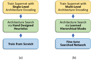
Figure 1: The pipelines of (a) existing weight sharing based NAS approaches such as DARTS [7] and SNAS [8]; and (b) HM-NAS (our approach).

2 Related Work

Designing high-quality neural networks requires domain knowledge and extensive experiences. To cut the labor intensity, there has been a growing interest in developing automated neural network design approaches through NAS. Pioneer works on NAS employ reinforcement learning (RL) or evolutionary algorithms to find the best architecture based on nested optimization [4, 1, 5, 6]. However, these approaches are incredibly expensive in terms of computation cost. For example, in [1], it takes 450 GPUs for four days to search for the best network architecture.

To reduce computation cost, many works adopt the weight sharing strategy where the weights of architecture candidates are inherited from a supernet that subsumes all the possible architecture candidates. To further reduce the computation cost, recent weight sharing based approaches such as DARTS [7] and SNAS [8] replace the discrete architecture search space with a continuous one and employ gradient descent to find the optimal architecture. However, these approaches restrict the continuous search space with hand designed heuristics, which could jeopardize the architecture search performance. Moreover, as discussed in [11, 12, 13], the bilevel optimization of architecture parameters and network weights used in existing weight sharing based approaches inevitably introduces bias to the architecture search process, making their architecture search results sub-optimal. Our approach is related to DARTS and SNAS in the sense that we both build upon the weight sharing strategy. However, our goal is to address the above limitations of existing approaches to achieve better architecture search performance.

NAS Approach	Architecture Encoding	Retrain from Scratch	Use Proxy
ENAS [4]	Operations	Yes	Yes
NASNet [1]	Operations	Yes	Yes
AmoebaNet [6]	Operations	Yes	Yes
NAONet [14]	Operations	Yes	Yes
ProxylessNAS [9]	Operations	Yes	No
FBNet [15]	Operations	Yes	No
DARTS [7]	Operations	Yes	Yes
SNAS [8]	Operations	Yes	Yes
HM-NAS	Operations & Edges	No	No

Table 1: Comparison between HM-NAS and other NAS approaches on a number of important dimensions.

Our approach is also related to ProxylessNAS [9]. ProxylessNAS formulates NAS as a model pruning problem. In our approach, the employed hierarchical masking scheme also prunes the redundant parts of the supernet to generate the optimal network architecture. The distinction is that ProxylessNAS focuses on pruning operations (referred to as path in [9]) of the supernet, while HM-NAS provides a more generalized model pruning mechanism which prunes the redundant operations, edges, and network weights of the supernet to derive the optimal architecture. Our approach is also similar to ProxylessNAS as being a proxyless approach. Rather than adopting a proxy strategy like [7, 8], which transfers the searched architecture to another larger network, both HM-NAS and ProxylessNAS directly search the architectures on target datasets without architecture transfer. However, unlike ProxylessNAS which involves retraining as the last step, HM-NAS eliminates the prolonged retraining process and replaces it with a fine-tuning process with the reuse of the unmasked pretrained supernet weights.

Table 1 provides a comparison between HM-NAS and relevant approaches on a number of important dimensions. The combination of the proposed multi-level architecture encoding and hierarchical masking techniques makes HM-NAS superior over many existing approaches. We quantify such superiority in §4.

3 Our Approach

3.1 Search Space and Supernet Design with Multi-Level Architecture Encoding

Following [6, 7, 8], we use a cell structure with an ordered sequence of nodes as our search space. The network is then composed of several identical cells which are stacked on top of each other. Specifically, a cell is represented using a directed acyclic graph (DAG) where each node $x$ in the DAG is a latent representation (e.g., a feature map in a convolutional network). A cell is set to have two input nodes, one or more intermediate nodes, and one output node. Specifically, the two input nodes are connected to the outputs of cells from two previous cells; each intermediate node is connected by all its predecessors; and the output node is the concatenation of all the intermediate nodes within the cell.

To build the supernet that subsumes all the possible architectures in the search space, existing works such as DARTS [7] and SNAS [8] associate each edge in the DAG with a mixture of candidate operations (e.g., convolution, pooling, identity) instead of a definite one. Moreover, each candidate operation of the mixture is assigned with a learnable variable (i.e., operation mixing weight) which encodes the importance of this candidate operation. As such, the mixture of candidate operations associated with a particular edge is represented as the softmax over all candidate operations:

$$\overline{o}(x)=\sum_{i=1}^{N}\frac{\text{exp}(\alpha_{i})}{\sum_{j}\text{exp}(\alpha_{j})}o_{i}(x)$$ (1)

where $\{o_{i}\}$ denote the set of $N$ candidate operations, $\{\alpha_{i}\}$ denote the set of $N$ real-valued operation mixing weights.

Although this supernet encodes the importance of different candidate operations within each edge, it does not provide a mechanism to encode the importance of different edges across the entire DAG. Instead, all the edges across the DAG are constrained to have the same importance. However, as we observed in our experiments (§4), loosening this constraint is able to help NAS find better architectures.

Motivated by this observation, in HM-NAS’s supernet, besides encoding the importance of each candidate operation within an edge, we introduce a separate set of learnable variables (i.e., edge mixing weights) to independently encode the importance of each edge across the DAG. As such, each intermediate node $x^{(i)}$ in the DAG is computed based on all of its predecessors as:

$$x^{(i)}=\sum_{j<i}\frac{\text{exp}(\beta^{(i,j)})}{\sum_{k<i}\text{exp}(\beta^{(i,k)})}\overline{o}(x^{(j)})$$ (2)

where $\beta^{(i,j)}$ denote the real-valued edge mixing weight for the directed edge $(i,j)$.

In summary, $\boldsymbol{\alpha}=\{\alpha_{i}\}$ encode the architecture at the operation level while $\boldsymbol{\beta}=\{\beta^{(i,j)}\}$ encode the architecture at the edge level. Therefore, we have constructed a supernet with multi-level architecture encoding where $\boldsymbol{\alpha}$ and $\boldsymbol{\beta}$ altogether encode the overall architecture of the network, and we refer to $\{\boldsymbol{\alpha},\boldsymbol{\beta}\}$ as the architecture parameters.

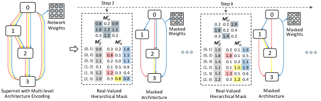
Figure 2: Illustration of the iterative hierarchical masking process on a single cell. In this example, each edge has 3 candidate operations marked using red, yellow, and blue color respectively. In each iteration, the real-valued hierarchical masks $\{\boldsymbol{M}^{r}_{\alpha},\boldsymbol{M}^{r}_{\beta},\boldsymbol{M}^{r}_{w}\}$ are passed through a deterministic thresholding function to obtain the corresponding binary masks (highlighted grids represent ‘1’, the rest represent ‘0’) that mask out redundant operations, edges, and weights of the supernet.

3.2 Training the Supernet

To train the multi-level encoded supernet, we follow [7] to jointly optimize the architecture parameters $\{\boldsymbol{\alpha},\boldsymbol{\beta}\}$ and the network weights $\boldsymbol{w}$ in a bilevel way via stochastic gradient descent with first or second-order approximation. Let $\mathcal{L}_{train}$ and $\mathcal{L}_{val}$ denote the training loss and validation loss respectively. The goal is to find $\{\boldsymbol{\alpha}^{*},\boldsymbol{\beta}^{*}\}$ that minimize $\mathcal{L}_{val}(\boldsymbol{\alpha},\boldsymbol{\beta},\boldsymbol{w}^{*})$, where $\boldsymbol{w}^{*}$ is obtained by minimizing the training loss $\boldsymbol{w}^{*}=\operatorname*{arg\,min}_{w}\mathcal{L}_{train}(\boldsymbol{\alpha}^{*},\boldsymbol{\beta}^{*},\boldsymbol{w})$. For the details of this bilevel optimization, please refer to [7] as we do not claim any new contribution on this part.

Here we want to emphasize two techniques that we find helpful in training our multi-level encoded supernet. First, due to insufficient training of network weights $\boldsymbol{w}$ at the beginning of the supernet training, the architecture parameters $\boldsymbol{\alpha}$ and $\boldsymbol{\beta}$ could be randomly selected. To avoid this, similar to [15], we adopt a warm start in training of $\boldsymbol{w}$ while freezing the training of $\boldsymbol{\alpha}$ and $\boldsymbol{\beta}$. Second, updating $\boldsymbol{\alpha}$ and $\boldsymbol{\beta}$ too frequently could lead to underfitting of $\boldsymbol{w}$. We solve this by triggering the optimization of $\boldsymbol{\alpha}$ and $\boldsymbol{\beta}$ stochastically rather than doing it constantly, with a probability of $p=\sigma(\textit{iter})$, where iter is the number of iterations and $\sigma(\cdot)$ is a monotonically non-increasing function that satisfies $\sigma(0)=1$. After a prolonged decrease, the probability $p$ may even be set to zero, i.e., no bilevel optimization is conducted any longer and only $\boldsymbol{w}$ is optimized.

3.3 Searching the Optimal Architecture via
Hierarchical Masking

Given the trained supernet, we formulate neural architecture search as a model pruning problem, and iteratively prune the redundant operations, edges, and network weights of the supernet in a hierarchical manner to derive the optimal architecture through a scheme which we refer to as hierarchical masking.

Figure 2 illustrates the iterative hierarchical masking process on a single cell. Specifically, we begin with the trained supernet as our base network, and initiate three types of real-valued masks for operations, edges, and network weights, respectively. These masks are passed through a deterministic thresholding function to obtain the corresponding binary masks. These generated binary masks are then elementwisely multiplied with the architecture parameters $\{\boldsymbol{\alpha}^{*},\boldsymbol{\beta}^{*}\}$ and network weights $\boldsymbol{w}^{*}$ of the supernet to generate a searched network. By iteratively training the real-valued masks through backpropagation combined with network binarization techniques [16] in an end-to-end manner, the binary masks learned in the end are able to mask out redundant operations, edges, and network weights in the supernet to derive the optimal architecture.

Formally, let $\boldsymbol{M}^{r}=\{\boldsymbol{M}^{r}_{\alpha},\boldsymbol{M}^{r}_{\beta},\boldsymbol{M}^{r}_{w}\}$ denote the real-valued hierarchical masks, where $\boldsymbol{M}^{r}_{\alpha},\boldsymbol{M}^{r}_{\beta},\boldsymbol{M}^{r}_{w}$ is the real-valued mask for operations, edges, and network weights, respectively. Architecture search is then reduced to finding $\boldsymbol{M}^{r*}$ which minimizes the training loss of the masked supernet:

$$\boldsymbol{M}^{r*}=\operatorname*{arg\,min}_{\boldsymbol{M}^{r}}\mathcal{L}(\mathcal{P}_{\boldsymbol{M}}(\boldsymbol{\alpha}^{*},\boldsymbol{\beta}^{*},\boldsymbol{w}^{*}))\vspace{-3mm}$$ (3)

$$\boldsymbol{M}=H(\boldsymbol{M}^{r}-\tau)$$ (4)

where $\boldsymbol{M}=\{\boldsymbol{M}_{\alpha},\boldsymbol{M}_{\beta},\boldsymbol{M}_{w}\}$ are the corresponding binary masks, $H(\cdot)$ is the Heaviside step function as the deterministic thresholding function, $\tau$ is the pre-defined threshold, and $\mathcal{P}(\cdot)$ is the elementwise projection function. In this work, we use elementwise multiplication for $\mathcal{P}(\cdot)$.

Even though the Heaviside step function in (4) is non-differentiable, we adopt the approximation strategy used in BinaryConnect [16] to approximate the gradients of real-valued masks $\boldsymbol{M^{r}}$ using the gradients of the binary masks $\boldsymbol{M}$, and thus update the real-valued masks $\boldsymbol{M^{r}}$ using the gradients of the binary masks $\boldsymbol{M}$. As shown in prior works [17, 16, 18], this strategy is effective because the gradients of $\boldsymbol{M}$ actually act as a regularizer or a noisy estimator of the gradients of $\boldsymbol{M^{r}}$. By doing this, the binary masks can be trained in an end-to-end differentiable manner.

3.4 Deriving the Final Model via Fine-Tuning

The hierarchical masking process in §3.3 outputs not only the optimal network architecture but also a set of optimized network weights. As such, we can derive the final model via fine-tuning instead of retraining the searched architecture from scratch. With the optimized network weights, the searched architecture is able to maintain comparable accuracy compared to the supernet (e.g., $\small{\sim}1\%$ loss on CIFAR-10), and thus acts as a significantly better starting point for fine-tuning. This not only ensures higher accuracy, but also replaces the prolonged retraining process with a more efficient fine-tuning process, as we will demonstrate in §4.2.

Input: multi-level architecture encoded supernet $\boldsymbol{\Theta}(\boldsymbol{\alpha},\boldsymbol{\beta},\boldsymbol{w})$, real-valued masks $\boldsymbol{M}^{r}_{\alpha}$, $\boldsymbol{M}^{r}_{\beta}$, $\boldsymbol{M}^{r}_{w}$, threshold $\tau$, deterministic thresholding function $H(\cdot)$, elementwise projection function $\mathcal{P}(\cdot)$

Output: {$\widehat{\boldsymbol{\Theta}}(\boldsymbol{\alpha^{*}},\boldsymbol{\beta^{*}},\boldsymbol{w^{*}}),\boldsymbol{M}^{*}_{\alpha},\boldsymbol{M}^{*}_{\beta},\boldsymbol{M}^{*}_{w}$}: the optimized searched model and binary masks

// supernet training

Initialize $\boldsymbol{\alpha}\leftarrow\boldsymbol{\alpha^{0}}$, $\boldsymbol{\beta}\leftarrow\boldsymbol{\beta^{0}}$, $\boldsymbol{w}\leftarrow\boldsymbol{w^{0}}$, $t\leftarrow 0$.

while not converge do

       Update $\boldsymbol{\beta}$ and $\boldsymbol{\alpha}$ by descending $\nabla_{\boldsymbol{\beta}}\mathcal{L}_{val}(\boldsymbol{\alpha^{*},\beta,w^{*}})$ and $\nabla_{\boldsymbol{\alpha}}\mathcal{L}_{val}(\boldsymbol{\alpha,\beta^{*},w^{*}})$ with a probability of $\sigma(t)$

      Update $\boldsymbol{w}$ by descending $\nabla_{\boldsymbol{w}}\mathcal{L}_{train}(\boldsymbol{\alpha^{*},\beta^{*},w})$

      $t\leftarrow t+1$

end while

// searching via hierarchical masking

Initialize $\boldsymbol{M}^{r}_{\alpha}\leftarrow\boldsymbol{M}^{0}_{\alpha}$, $\boldsymbol{M}^{r}_{\beta}\leftarrow\boldsymbol{M}^{0}_{\beta}$, $\boldsymbol{M}^{r}_{w}\leftarrow\boldsymbol{M}^{0}_{w}$

while not converge do

       Feed forward and loss calculation with $\mathcal{P}_{H(\boldsymbol{M}^{r}_{w}-\tau)}(\boldsymbol{w^{*}})$, $\mathcal{P}_{H(\boldsymbol{M}^{r}_{\alpha}-\tau)}(\boldsymbol{\alpha}^{*})$, $\mathcal{P}_{H(\boldsymbol{M}^{r}_{\beta}-\tau)}(\boldsymbol{\beta}^{*})$

      Update $\boldsymbol{M}^{r}$ by descending $\nabla_{H(\boldsymbol{M}^{r}-\tau)}\mathcal{L}_{train}(\mathcal{P}_{{\boldsymbol{M}}}(\boldsymbol{\alpha}^{*},\boldsymbol{\beta}^{*},\boldsymbol{w^{*}}))$

end while

// fine-tuning the searched network

Initialize $\boldsymbol{w}\leftarrow\boldsymbol{w^{*}}$. Construct searched network $\widehat{\boldsymbol{\Theta}}(\boldsymbol{\alpha}^{*},\boldsymbol{\beta}^{*},\boldsymbol{w})$ masked by $\boldsymbol{M}^{*}_{\alpha},\boldsymbol{M}^{*}_{\beta},\boldsymbol{M}^{*}_{w}$.

while not converge do

       Update unmasked $\boldsymbol{w}$ by descending $\nabla_{\boldsymbol{w}}\mathcal{L}_{train}(\mathcal{P}_{{\boldsymbol{M}}^{*}}(\boldsymbol{\alpha}^{*},\boldsymbol{\beta}^{*},\boldsymbol{w}))$

end while

Algorithm 1 HM-NAS

4 Experiments and Results

We evaluate the performance of HM-NAS and compare it with state-of-the-arts NAS approaches on two benchmark datasets: CIFAR-10 (§4.2) and ImageNet (§4.3). Moreover, we have conducted a series of ablation studies that validate the importance and effectiveness of the proposed multi-level architecture encoding scheme and hierarchical masking scheme incorporated in the design of HM-NAS (§4.4). Finally, we provide an in-depth analysis on the architecture found by HM-NAS (§4.5).

4.1 Experimental Setup

We use 3 cells and 36 initial channels to build the supernet for CIFAR-10, and 5 cells and 24 initial channels for ImageNet. Following DARTS [7], our cell consists of 7 nodes in all the experiments. The input nodes, i.e., the first and second nodes of cell $k$ is the output of cell $k-1$ and $k-2$, respectively. The output node is the depthwise concatenation of all the intermediate nodes. We include the following operations: $3\times 3$ and $5\times 5$ separable convolutions, $3\times 3$ and $5\times 5$ dilated separable convolutions, $3\times 3$ max pooling and average pooling, and identity. ReLU-Conv-BN triplet is adopted for convolutional operations except the first convolutional layer (Conv-BN), and each separable convolution is applied twice. The default stride is 1 for all operations unless the output size is changed. The experiments are conducted using a single NVIDIA Tesla V100 GPU.

4.2 Results on CIFAR-10

Training Details. We begin with training the supernet for 100 epochs with batch size 128. In each epoch, we first train weights $\boldsymbol{w}$ on $80\%$ of the training set using SGD with momentum. The initial learning rate is 0.1 with decay following a cosine decaying schedule. The momentum is 0.9 and weight decay is 3e-4. Architecture parameters $\boldsymbol{\alpha}$, $\boldsymbol{\beta}$ are randomly initialized and scaled by 1e-3. Next, We train $\boldsymbol{\alpha}$ and $\boldsymbol{\beta}$ on the rest $20\%$ of the training set with Adam optimizer [19] with the learning rate of 3e-4 and weight decay of 1e-3. We empirically observe more stable training process when using Adam for optimizing the architecture parameters, which is also used in [7]. Following [15], we postpone the training of $\boldsymbol{\alpha}$ and $\boldsymbol{\beta}$ by 10 epochs to warm up $\boldsymbol{w}$ first. The supernet training takes 7.5 hours (or 30 hours for the second-order approximation). Once the supernet is trained, we perform 20 epochs of neural architecture search via hierarchical masking using the entire training set. Hierarchical masks $\boldsymbol{M}^{r}_{\alpha},\boldsymbol{M}^{r}_{\beta},\boldsymbol{M}^{r}_{w}$ are initialized as 1e-2. They are trained using the Adam optimizer with an initial learning rate of 1e-4 for $\boldsymbol{M}^{r}_{w}$ and 1e-5 for $\boldsymbol{M}^{r}_{\alpha}$ and $\boldsymbol{M}^{r}_{\beta}$, which is decayed by a factor of 10 after 10 epochs. The binarizer threshold $\tau$ (Equation 4) is 5e-3. The hierarchical mask training takes 3.5 hours. Lastly, the masked network is fine-tuned for 200 epochs for 9.6 hours with cutout [20].

Architecture Evaluation. Table 2 shows our evaluation results on CIFAR-10 where ‘c/o’ denotes cutout adapted from [20]. The test error of HM-NAS is on par with state-of-the-art NAS methods. Notably, HM-NAS achieves this by using the fewest parameters among all methods. Specifically, HM-NAS only uses 1.8M parameters, which is $1.4\times$ to $3.2\times$ fewer compared to others.

Architecture	Test Error (%)	Params (M)	Search Cost (GPU days)	Train Cost (GPU days)	Total Cost (GPU days)	Search Method
DenseNet-BC [21]	3.46	25.6	-	-	-	manual
ENAS + c/o [4]	2.89	4.6	0.45	(630 epochs)†	-	RL
NASNet-A + c/o [1]	2.65	3.3	3150	-	-	RL
SNAS + c/o [8]	2.85	2.8	1.5	1.5 (600 epochs)	3	gradient-based
ProxyLess-G + c/o	2.08	5.7	4*	(600 epochs)	-	gradient-based
AmoebaNet-A + c/o [6]	3.34 $\pm$ 0.06	3.2	3150	-	-	evolution
AmoebaNet-B + c/o [6]	2.55 $\pm$ 0.05	2.8	3150	-	-	evolution
DARTS (1st order) + c/o [7]	3.00 $\pm$ 0.14	3.3	1.5*	2† (600 epochs)	3.5	gradient-based
DARTS (2nd order) + c/o [7]	2.76 $\pm$ 0.09	3.3	4*	2† (600 epochs)	6	gradient-based
HM-NAS (1st order) + c/o	2.78 $\pm$ 0.07	1.8	0.45	0.4 (200 epochs)	0.85	gradient-based
HM-NAS (2nd order) + c/o	2.41 $\pm$ 0.05	1.8	1.4	0.4 (200 epochs)	1.8	gradient-based
* Results obtained from authors’ official response in openreview.
† Results obtained using code publicly released by the authors.

Table 2: Comparison with state-of-the-arts on CIFAR-10.

Performance at Different Training Stages. Table 3 breaks down the complete architecture search process of HM-NAS and shows the performance of HM-NAS at different stages. Specifically, compared to the supernet, the searched network (derived after hierarchical masking) loses only $\small{\sim}1\%$ accuracy with $40\%$ less parameters. Although directly using this searched network is not optimal (with test error $5.14\%$), it does provide a good initialization for fine-tuning, which leads to lower test error (from $5.14\%$ to $2.41\%$).

Architecture	Test Error (%)	Params (M)	Params Reduction (%)
Supernet	4.2	3	-
Searched Network	5.14	1.8	40
Searched Network + Fine-Tuning	2.41	1.8	40

Table 3: Performance of HM-NAS at different architecture search stages.

Architecture Search Cost Analysis. To find the optimal architecture, HM-NAS only uses 0.85 or 1.8 GPU days, which is significantly faster compared to all other NAS methods. To understand why HM-NAS is efficient, we compare the complete architecture search process of HM-NAS to DARTS. Figure 3 illustrates the training curve of HM-NAS (in blue color) and DARTS (in red color) during the complete architecture search process on CIFAR-10. Specifically, both HM-NAS and DARTS use the first 100 epochs to train the supernet with the same train/validation dataset split. Due to multi-level architecture encoding, HM-NAS is able to achieve better test results after 100 epochs. Then, DARTS transfers the learned cell to build a larger network and retrains it from scratch. This process takes approximately 600 epochs to converge. In contrast, from 100 epoch to 120 epoch and onward, HM-NAS performs architecture search via hierarchical masking and fine-tuning, respectively. This process only takes 220 epochs to converge, which is $2.7\times$ faster compared to DARTS.

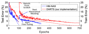
Figure 3: Training curves of HM-NAS (in blue color) and DARTS (in red color) on CIFAR-10. Solid lines denote test errors (y-axis on the left); dashed lines denote training errors (y-axis on the right).

4.3 Results on ImageNet

We conduct experiments on ImageNet 1000-class [22] classification task, where input image size is $224\times 224$. The dataset has around 1.28M training images and we test on the 50k validation images.

Training Details. We adopt the small computation regime (e.g., MobileNet-V1 [23]) in the experiments. Following [15], 100 classes from the original 1,000 classes of ImageNet is randomly sampled to train the supernet for 100 epochs with batch size 128. It takes around one GPU day to finish the supernet training. Once the supernet is trained, the hierarchical masking is then performed with the same optimization settings mentioned in §4.2. The hierarchical masking process takes around one GPU day to finish. Lastly, the searched network is fine-tuned on the entire ImageNet training dataset (with 1,000 classes) for $60$ epochs with initial learning rate 1e-2 then decreased to 1e-3 at the epoch 30. This phase takes around $3$ GPU days to finish.

Architecture Evaluation. Table 4 shows our evaluation results on ImageNet. The result is comparable to DARTS, considering that we adopt the exact same search space in DARTS [7], which uses the operations incorporated in MobileNet-V1 [23]. Notably, we achieve comparable results to the state-of-the-art gradient-based NAS approaches [8, 7] with 1.2$\times$ to 1.3$\times$ less parameters and 1.08$\times$ to 1.2$\times$ less FLOPs. With a larger supernet and better candidate operations such as the ones used in MobileNet-V2 [24], We believe that the results could be further improved.

Architecture	Top-1 Acc. (%)	Params (M)	FLOPs (M)
MobileNet-V1 [23]	70.6	4.2	569
MobileNet-V2 [24]	74.7	6.9	585
NASNet-A [1]	74.0	5.3	564
Amoeba-A [6]	74.5	5.1	555
DARTS [7]	73.3	4.7	574
SNAS [8]	72.7	4.3	522
HM-NAS	73.4	3.6	482

Table 4: Comparison with state-of-the-arts on ImageNet.

4.4 Ablation Studies

In this section, we conduct a series of ablation studies to demonstrate the superiority of the design of HM-NAS. The ablation studies are conducted on CIFAR-10 with second-order derivative introduced in Table 2.

Comparison to Single-Level Architecture Encoding. To demonstrate the superiority of the proposed multi-level architecture encoding scheme over single-level architecture encoding, we compare the single-level encoded network against the multi-level encoded network, both with hand designed heuristics (by replacing each mixed operation with the most likely operation and taking the top-2 confident edges from distinct nodes). As shown in Table 5, the multi-level architecture encoding achieves $2.7$% test error, giving $0.4\%$ accuracy improvement over the single-level one.

Comparison to Hand Designed Heuristics. To demonstrate the superiority of learned hierarchical masks over hand designed heuristics, we compare the multi-level encoded network with learned hierarchical masks against the one with hand designed heuristics. As shown in Table 5, the hierarchical masks achieve $2.41$% test error, providing about $0.3\%$ accuracy improvement over hand designed heuristics.

Comparison to Random Architectures. As discussed in [11, 25], random architecture is also a competitive choice. Therefore, we perform a random architecture search from the same supernet for 18 times. As shown in Table 6, the average test error of random architecture is $3.41\%$. This is competitive to the test error of single-level encoded network ($3.1\%$ in Table 5), whose search space is constrained by hand designed heuristics. Similar findings are also observed in [11]. In contrast, HM-NAS outperforms the random architecture by $1\%$ in test error with 3$\times$ less training epochs. This is because with multi-level architecture encoding and hierarchical masking, the search space is significantly enlarged, making it challenging for random search to find a competitive network.

Comparison to Random Initialization. As our final ablation study, to demonstrate the superiority of unmasked network weights obtained from hierarchical masking over random weights, we randomly initialize the weights of the searched network (same architecture as HM-NAS) and train it for $600$ epochs on par with the training setup in DARTS. We run 5 times of random initialization, each running the same number of epochs. As shown in Table 6, the average test error of random initialization is 2.95%, which is comparable to DARTS but considerably higher than HM-NAS. This result indicates that a good initialization for the searched network is critical for obtaining the best-performing results and fast convergence.

Architecture Encoding	Derived Rule	Test Error (%)	Params (M)
Single-Level ($\boldsymbol{\alpha}$)	Hand Designed Heuristics	3.1	2.5
Multi-Level ($\boldsymbol{\alpha}$, $\boldsymbol{\beta}$)	Hand Designed Heuristics	2.7	2.1
Multi-Level ($\boldsymbol{\alpha}$, $\boldsymbol{\beta}$)	Learned Hierarchical Masks	2.41	1.8

Table 5: Comparison to single-level architecture encoding and hand designed heuristics.

Architecture	Test Error (%)	Params (M)	Train Cost (epochs)
Random Architecture	3.41 $\pm$ 0.15	2.1	600
Random Initialization ‡	2.95 $\pm$ 0.08	1.8	600
HM-NAS	2.41 $\pm$ 0.05	1.8	200
‡ Same architecture as HM-NAS + c/o with random initialized weights.

Table 6: Comparison to random architectures and random initialization.

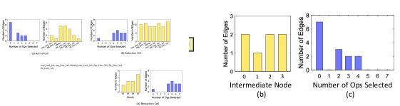
Figure 4: Details of learned cell for CIFAR-10. (a) cell structure. (b) number of input edges of four intermediate nodes. (c) histogram of the number of edges w.r.t the number of operations selected.

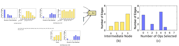
Figure 5: Details of learned cell for ImageNet. (a) cell structure. (b) number of input edges of four intermediate nodes. (c) histogram of the number of edges w.r.t the number of operations selected.

4.5 Searched Architecture Analysis

Finally, we provide an in-depth analysis on the network architecture found by HM-NAS. We have the following three important observations.

Different Learned Importance for Different Edges. Figure 4(a) and Figure 5(a) illustrate the details of the learned cell for CIFAR-10 and ImageNet respectively, where the importance of edge, i.e., edge mixing weight $\beta^{(i,j)}$, is marked above every edge. Unlike DARTS in which each edge has the same hard-coded importance, due to multi-level architecture encoding, the best-performing cell found by HM-NAS has different learned importance for different edges across the cell. Moreover, we find that edges connecting to later intermediate nodes have higher importance than early intermediate nodes. One possible explanation is that during cell construction, each intermediate node is ordered and is derived from its predecessors by accumulating information passed from its predecessors. Hence, it has more influence on the output of the cell, which is reflected by the higher importance learned through our approach. Once the importance of the edge is no longer heuristically determined but automatically learned, the multi-level architecture encoding provides a more flexible way to encode the entire supernet architecture and thus provides us with a better superset for architecture search.

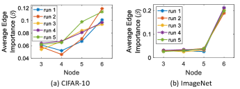
Figure 6: Robustness of learned edge importance of (a) CIFAR-10 and (b) ImageNet. The learned importance of different edges does not strongly depend on initialization.

Robustness of Learned Edge Importance. We repeat the experiments 5 times with random seeds on both CIFAR-10 and ImageNet datasets, and report the (per run) averaged incoming edge importance in each immediate node with the best validation performance of the architecture over epochs (we keep track of the most recent architectures). As shown in Figure 6, we observe that the learned importance of different edges does not strongly depend on initialization: even if the initial weights are randomly initialized, after the search process completes, the later intermediate nodes always have higher importance than earlier nodes.

More Flexible Architectures. Figure 4(b) and Figure 5(b) show the number of input edges connecting to each intermediate node, while Figure 4(c) and Figure 5(c) show the histogram of the number of edges w.r.t the number of operations selected (e.g. the third bar from the left shows that three edges have two associated operations). Unlike DARTS in which each intermediate node is hard coded to have exactly two input edges and each edge is hard coded to have exactly one operation, the best-performing cell found by HM-NAS has intermediate nodes which have more ($\geq$ 2) incoming edges, and edges are associated with zero (the edge is removed) or multiple ($\geq$ 1) operations. This observation suggests that HM-NAS is able to find more flexible architectures that existing weight sharing based NAS approaches are not able to discover.

In principle, other constraints such as the number of cells, the number of channels, the number of nodes in a cell, and the combination operation (e.g. sum, concatenation) can all be further relaxed by the proposed multi-level architecture encoding and hierarchical masking schemes. We leave these explorations as our future work.

5 Conclusion

We present an efficient NAS approach named HM-NAS that generalizes existing weight sharing based NAS approaches. HM-NAS incorporates a multi-level architecture encoding scheme to enable an architecture candidate to have arbitrary numbers of edges and operations with different importance. The learned hierarchical masks not only select the optimal numbers of edges, operations and important network weights, but also help correct the architecture search bias caused by bilevel optimization in supernet training. Experiment results show that, compared to state-of-the-arts, HM-NAS is able to achieve competitive accuracy on CIFAR-10 and ImageNet with improved architecture search efficiency.

6 Acknowledgement

This work was partially supported by NSF Awards CNS-1617627 and PFI:BIC-1632051.

References

- [1] Barret Zoph, Vijay Vasudevan, Jonathon Shlens, and Quoc V Le. Learning transferable architectures for scalable image recognition. In CVPR, pages 8697–8710, 2018.
- [2] Yukang Chen, Tong Yang, Xiangyu Zhang, Gaofeng Meng, Chunhong Pan, and Jian Sun. Detnas: Neural architecture search on object detection. arXiv preprint arXiv:1903.10979, 2019.
- [3] Vladimir Nekrasov, Hao Chen, Chunhua Shen, and Ian Reid. Fast neural architecture search of compact semantic segmentation models via auxiliary cells. In CVPR, pages 9126–9135, 2019.
- [4] Hieu Pham, Melody Guan, Barret Zoph, Quoc Le, and Jeff Dean. Efficient neural architecture search via parameters sharing. In ICML, 2018.
- [5] Bowen Baker, Otkrist Gupta, Nikhil Naik, and Ramesh Raskar. Designing neural network architectures using reinforcement learning. In ICLR, 2017.
- [6] Esteban Real, Alok Aggarwal, Yanping Huang, and Quoc V Le. Regularized evolution for image classifier architecture search. In AAAI, 2019.
- [7] Hanxiao Liu, Karen Simonyan, and Yiming Yang. Darts: Differentiable architecture search. In ICLR, 2019.
- [8] Sirui Xie, Hehui Zheng, Chunxiao Liu, and Liang Lin. Snas: stochastic neural architecture search. In ICLR, 2019.
- [9] Han Cai, Ligeng Zhu, and Song Han. Proxylessnas: Direct neural architecture search on target task and hardware. In ICLR, 2019.
- [10] Andrew Brock, Theodore Lim, James M. Ritchie, and Nick Weston. Smash: One-shot model architecture search through hypernetworks. ICLR, 2018.
- [11] Christian Sciuto, Kaicheng Yu, Martin Jaggi, Claudiu Musat, and Mathieu Salzmann. Evaluating the search phase of neural architecture search. arXiv preprint arXiv:1902.08142, 2019.
- [12] Gabriel Bender, Pieter-Jan Kindermans, Barret Zoph, Vijay Vasudevan, and Quoc Le. Understanding and simplifying one-shot architecture search. In ICML, pages 549–558, 2018.
- [13] Zichao Guo, Xiangyu Zhang, Haoyuan Mu, Wen Heng, Zechun Liu, Yichen Wei, and Jian Sun. Single path one-shot neural architecture search with uniform sampling. arXiv preprint arXiv:1904.00420, 2019.
- [14] Renqian Luo, Fei Tian, Tao Qin, Enhong Chen, and Tie-Yan Liu. Neural architecture optimization. In Advances in neural information processing systems, pages 7816–7827, 2018.
- [15] Bichen Wu, Xiaoliang Dai, Peizhao Zhang, Yanghan Wang, Fei Sun, Yiming Wu, Yuandong Tian, Peter Vajda, Yangqing Jia, and Kurt Keutzer. Fbnet: Hardware-aware efficient convnet design via differentiable neural architecture search. In Proceedings of the IEEE Conference on Computer Vision and Pattern Recognition, pages 10734–10742, 2019.
- [16] Matthieu Courbariaux, Yoshua Bengio, and Jean-Pierre David. Binaryconnect: Training deep neural networks with binary weights during propagations. In Advances in neural information processing systems, pages 3123–3131, 2015.
- [17] Arun Mallya, Dillon Davis, and Svetlana Lazebnik. Piggyback: Adapting a single network to multiple tasks by learning to mask weights. In ECCV, pages 67–82, 2018.
- [18] Itay Hubara, Matthieu Courbariaux, Daniel Soudry, Ran El-Yaniv, and Yoshua Bengio. Binarized neural networks. In Advances in neural information processing systems, pages 4107–4115, 2016.
- [19] Diederik P Kingma and Jimmy Ba. Adam: A method for stochastic optimization. ICLR, 2015.
- [20] Terrance DeVries and Graham W Taylor. Improved regularization of convolutional neural networks with cutout. arXiv preprint arXiv:1708.04552, 2017.
- [21] Gao Huang, Zhuang Liu, Laurens Van Der Maaten, and Kilian Q Weinberger. Densely connected convolutional networks. In CVPR, pages 4700–4708, 2017.
- [22] Jia Deng, Wei Dong, Richard Socher, Li-Jia Li, Kai Li, and Li Fei-Fei. ImageNet: A Large-Scale Hierarchical Image Database. In CVPR, 2009.
- [23] Andrew G Howard, Menglong Zhu, Bo Chen, Dmitry Kalenichenko, Weijun Wang, Tobias Weyand, Marco Andreetto, and Hartwig Adam. Mobilenets: Efficient convolutional neural networks for mobile vision applications. arXiv preprint arXiv:1704.04861, 2017.
- [24] Mark Sandler, Andrew Howard, Menglong Zhu, Andrey Zhmoginov, and Liang-Chieh Chen. Mobilenetv2: Inverted residuals and linear bottlenecks. In CVPR, pages 4510–4520, 2018.
- [25] Liam Li and Ameet Talwalkar. Random search and reproducibility for neural architecture search. arXiv preprint arXiv:1902.07638, 2019.