Asymptotic dynamics of three-dimensional bipolar ultrashort electromagnetic pulses in an array of semiconductor carbon nanotubes

Abstract

We study the propagation of three-dimensional bipolar ultrashort electromagnetic pulses in an array of semiconductor carbon nanotubes at times much longer than the pulse duration, yet still shorter than the relaxation time in the system. The interaction of the electromagnetic field with the electronic subsystem of the medium is described by means of Maxwell’s equations, taking into account the field inhomogeneity along the nanotube axis beyond the approximation of slowly varying amplitudes and phases. A model is proposed for the analysis of the dynamics of an electromagnetic pulse in the form of an effective equation for the vector potential of the field. Our numerical analysis demonstrates the possibility of a satisfactory description of the evolution of the pulse field at large times by means of a three-dimensional generalization of the sine-Gordon and double sine-Gordon equations.

1 Introduction

Carbon nanotubes—quasi-one-dimensional macromolecules of carbon [1, 2, 3] —are now considered to be one of the most promising materials with a high potential of applicability in the development of the elemental base for modern electronics. From the point of view of applications in optoelectronics, it is of particular interest to study the properties of nanotubes with respect to the peculiarity of their electronic structure. The non-parabolicity of the dispersion law for the conduction electrons of nanotubes [1, 2, 3] (i.e. the energy dependency on the quasi-momentum) determines the essential nonlinearity of their response to the action of the electromagnetic field [4]. This circumstance provides the principal possibility of observing various unique electromagnetic phenomena in structures based on carbon nanotubes, including nonlinear diffraction and self-focusing of laser beams [5, 6].

The successes of modern laser technologies in the field of the formation of powerful electromagnetic radiation with given parameters, including extremely short laser pulses with durations corresponding to several half-cycles of field oscillations [7, 8, 9, 10, 11, 12, 13, 14, 15, 16], provides the impetus for further comprehensive investigations in the field of light-matter interaction, the results of which can subsequently form the basis for the newest elements of modern electronics. In particular, one of such promising areas of research is the study of the generation and propagation of laser beams and extremely short spatio-temporal pulses in various media (e.g., see [17, 18, 19, 20, 21, 22, 23, 24, 25, 26, 27, 28, 29, 30, 31]) including arrays of carbon nanotubes [32].

The possibility of stable propagation of ultrashort electromagnetic pulses in arrays of carbon nanotubes was first theoretically established in [32, 33] in a one-dimensional model, and was subsequently studied in a two-dimensional model [34, 35, 36, 37, 38] in the framework of the homogeneous field approximation along the axes of nanotubes. The approach used in the above works did not take into account the effects associated with the inhomogeneity of the field along the nanotube axes; therefore, in order to obtain a more realistic description of field evolution, the mathematical model was generalized to the case of two and three spatial dimensions, and was supplemented by equations that take into account the redistribution of the charge density in the system under the influence of the field inhomogeneity along the axis of the nanotubes. As a result, the peculiarities of propagation of solitary electromagnetic waves in arrays of carbon nanotubes were studied both in two-dimensional [39, 40] and three-dimensional [41, 42, 43] models, taking into account the effect of localization of the field along the nanotube axes. In the course of numerical experiments carried out within the framework of these studies, the possibility of stable propagation of bipolar ultrashort electromagnetic pulses in the form of bipolar “breather-like” light bullets at distances significantly exceeding the characteristic dimensions of the pulses along the direction of their motion was confirmed.

To date, a large amount of information has already been accumulated as a result of extensive studies of various aspects of the interaction of extremely short laser pulses with arrays of nanotubes, but there are still numerous questions that require further clarification. In particular, from the point of view of possible practical applications, it is instrumental to study the evolution of the electromagnetic pulse field in an array of nanotubes at time intervals that significantly exceed the characteristic pulse duration, but that are still shorter than the relaxation time in the system. Such a problem of considering the dynamics of a pulse at times several orders of magnitude greater than its duration naturally arises in the case of the propagation of extremely short pulses with a characteristic duration $\Delta t_{\rm{pulse}}\sim 10^{-15}-10^{-14}$ s in the medium with the relaxation time $t_{\rm{rel}}\sim 10^{-12}-10^{-11}$ s, which is quite achievable with modern technologies for fabricating nanotube structures. A study of the asymptotic dynamics of an ultimately short pulse at large times was carried out earlier in [44] for a one-dimensional model in the homogeneous field approximation along the nanotube axis. However, the results obtained within that simplified framework cannot always be automatically extrapolated to the behavior of a pulse in a model containing more than one spatial dimension. Peculiarities of the behavior of a pulse in a non-one-dimensional geometry can occur owing to the influence of the transverse effects associated with the diffraction spreading of the wave packet. In this connection, it seems expedient to solve the problem of modeling the evolution of parameters of an extremely short laser pulse in an array of carbon semiconductor nanotubes, taking into account the three-dimensional localization of the field.

2 System configuration and key assumptions

In this paper, we consider the propagation of a solitary electromagnetic wave in the bulk array of single-walled semiconductor carbon nanotubes (CNTs) embedded in a homogeneous dielectric medium. The nanotubes considered here are of the “zigzag" type $(m,0)$, where the number $m$ (not a multiple of three for semiconductor nanotubes) determines the nanotube radius $R=mb\sqrt{3}/2\pi$, and $b=1.42\times 10^{-8}\mathrm{~{}cm}$ is the distance between neighboring carbon atoms [1, 2, 3]. The CNTs are supposed to be arranged in such a way that their axes are parallel to the common $x$-axis, and distances between adjacent nanotubes are much larger than their diameter, so that we neglect the interaction between them. This latter assumption allows us to consider the system as an electrically quasi-one-dimensional one, in which electron tunneling between neighboring nanotubes can be neglected, and electrical conductivity is possible only along the axis of nanotubes.

We define the configuration of the system in such a way that the pulse propagates through the nanotube array in a direction perpendicular to their axes (that is, for definiteness along the $z$-axis), and the electric component of the wave field ${\bf E}=\{E,0,0\}$ is collinear with the $x$-axis (see Fig. 1).

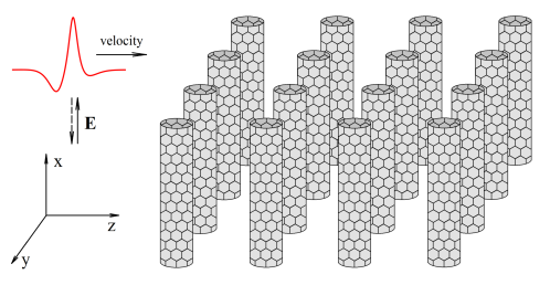
Figure 1: Schematic diagram of the considered system with the associated coordinate system.

We note that for a wide range of values of the system parameters, the characteristic distance at which an appreciable change in the field of a bipolar electromagnetic pulse occurs is significantly greater than the distance between neighboring nanotubes, and also the characteristic length of the conduction electron path along the axis of the nanotubes. For example, for a nanotube radius $R\approx 2.74\times 10^{-8}\mathrm{~{}cm}$ and $m=7$, the characteristic distance between them (sufficient to exclude the overlap of the electron wave functions of neighboring nanotubes)—even if substantially exceeding the value of the radius $R$—will be negligibly small in comparison with the characteristic wavelength of the electromagnetic radiation in the system. In particular, in the case of infrared electromagnetic radiation this assumption remains valid. With this approximation, the nanotube array, which is a discrete structure at the microscopic level, can nevertheless be considered as a continuous medium at the considered wavelength scale of electromagnetic radiation propagating in it.

Another important assumption that we adopt in this paper concerns the magnitudes of the time duration of the electromagnetic pulse, $\Delta t_{\rm{pulse}}$, the relaxation time of the conduction current along the nanotube axis, $t_{\rm{rel}}$, and also the time interval for observing the evolution of the field in the system, $\Delta t$. Specifically, we assume that the observation time $\Delta t$ is much longer than the pulse duration $\Delta t_{\rm{pulse}}$, but still shorter than the relaxation time $t_{\rm{rel}}$, namely $\Delta t_{\rm{pulse}}\ll\Delta t<t_{\rm{rel}}$.

Given the orientation of the coordinate system axes relative to the nanotube axis chosen above (see Fig. 1), the electron energy spectrum for carbon nanotubes takes the form

$$\epsilon(p_{x},s)=\gamma_{0}\sqrt{1+4\cos\left(p_{x}\frac{d_{x}}{\hbar}\right)\cos\left(\pi\frac{s}{m}\right)+4\cos^{2}\left(\pi\frac{s}{m}\right)},$$ (1)

where the electron quasimomentum is $\mathbf{p}=\left\{p_{x},s\right\}$, $s$ being an integer characterizing the momentum quantization along the perimeter of the nanotube, $s=1,2,\dots,m$, $m$ is the number of hexagonal carbon cycles, forming the circumference of a nanotube, $\gamma_{0}$ is the overlap integral, and where $d_{x}=3b/2$ [1, 2, 3].

3 Evolution of the system parameters

3.1 Complete set of equations

As we showed earlier (see, for example [42, 43] and references therein), the evolution of the electromagnetic field in an array of nanotubes is described by Maxwell’s equations for the vector and scalar potentials, ${\bf A}=\{A,0,0\}$ and $\phi$, together with the continuity equation [45, 46] for the current density ${\bf j}=\{j,0,0\}$, which is calculated according to the approach proposed in [47, 48]. As a result, the set of evolutionary equations consists of three of them: for the vector and scalar potentials, ${\bf A}=\{A,0,0\}$ and $\phi$, respectively, and for the conduction electron density $n$.

The equation describing the evolution of the vector potential of a self-consistent electromagnetic field in an array of nanotubes has the form [42]

$$\frac{\partial^{2}\Psi}{\partial\tau^{2}}-\left(\frac{\partial^{2}\Psi}{\partial\xi^{2}}+\frac{\partial^{2}\Psi}{\partial\upsilon^{2}}+\frac{\partial^{2}\Psi}{\partial\zeta^{2}}\right)+\eta\sum_{r=1}^{\infty}G_{r}\sin\left[r\left(\Psi+\int\limits_{0}^{\tau}\frac{\partial\Phi}{\partial\xi}d\tau^{\prime}\right)\right]=0.$$ (2)

Here, we use the following notation: $\Psi=Aed_{x}/\left(c\hbar\right)$ is the projection of the dimensionless vector potential onto the nanotube axis; $\Phi=\phi\sqrt{\varepsilon}ed_{x}/(c\hbar)$ is the dimensionless scalar potential; $\varepsilon$ is the average relative permittivity of the sample (see, for example [49]); $\eta=n/n_{\rm{bias}}=\eta(\xi,\upsilon,\zeta,\tau)$ is the reduced (dimensionless) distribution of conduction electron density, with n the instantaneous value of the conduction electrons concentration at an arbitrary point of the sample bulk; $n_{\rm{bias}}$ is the concentration of conduction electrons in the sample in the absence of an electromagnetic field (that is, essentially a constant component of the concentration). The coefficients $G_{r}$ are the dimensionless quantities that decrease with increasing $r$ [42]; $\tau=\omega_{0}t/\sqrt{\varepsilon}$ is the scaled time; $\xi=x\omega_{0}/c$, $\upsilon=y\omega_{0}/c$ and $\zeta=z\omega_{0}/c$ are the dimensionless coordinates. The quantity $\omega_{0}=2|e|d_{x}\hbar^{-1}\sqrt{\pi\gamma_{0}n_{\rm{bias}}}$ has the meaning of the characteristic frequency of the electron subsystem of nanotubes ($e<0$ is the electron charge).

The equation describing the spatio-temporal evolution of the concentration of conduction electrons in an array of nanotubes has the form [39, 40, 41, 42, 43]

$$\frac{\partial\eta}{\partial\tau}=\alpha\sum_{r=1}^{\infty}G_{r}\frac{\partial}{\partial\xi}\left\{\eta\sin\left[r\left(\Psi+\int\limits_{0}^{\tau}\frac{\partial\Phi}{\partial\xi}d\tau^{\prime}\right)\right]\right\},$$ (3)

with $\alpha=d_{x}\gamma_{0}\sqrt{\varepsilon}/c\hbar$. This equation determines the change in the electron concentration under the effect of a self-consistent electromagnetic field in the array of nanotubes. We emphasize that the inhomogeneity (localization) of the field only along the $x$-axis can cause non-stationarity and dynamic spatial inhomogeneity of the electron concentration in the sample, due to the presence of conductivity only along the axis of the nanotubes. In this case, the inhomogeneity of the field along the directions orthogonal to the axes of the nanotubes will not contribute to the redistribution of the electron concentration due to the negligible overlap of the electron wave functions of neighboring nanotubes and the absence of conductivity in the $yOz$–plane.

As was shown earlier in [39, 40, 41, 42, 43], the equation describing the evolution of the scalar potential of a field in an array of nanotubes has the form

$$\frac{\partial^{2}\Phi}{\partial\tau^{2}}-\left(\frac{\partial^{2}\Phi}{\partial\xi^{2}}+\frac{\partial^{2}\Phi}{\partial\upsilon^{2}}+\frac{\partial^{2}\Phi}{\partial\zeta^{2}}\right)=\beta(\eta-\eta_{0}),$$ (4)

where $\beta=1/\alpha=c\hbar/\left(d_{x}\gamma_{0}\sqrt{\varepsilon}\right)$, and $\eta_{0}=n_{0}/n_{\rm{bias}}=\eta(\xi,\upsilon,\zeta,\tau_{0})$ is the reduced (dimensionless) value of the concentration of conduction electrons at a given point in space at the initial instant of time $\tau_{0}$ in the absence of the field. In the simplest particular case corresponding to an initially homogeneous sample ($n_{0}=n_{\rm{bias}}$), we have $\eta_{0}=1$.

Thus, the evolution of the field in the array of nanotubes is described by the set of Eqs. (2)–(4). These equations describe a self-consistent system of physical parameters, $\Psi$, $\Phi$, and $\eta$, the dynamics of which reflect the mutual influence of the electromagnetic field and the electronic subsystem of the nanotubes array (self-consistent light-matter interaction).

3.2 Effective equation for the vector potential

When considering the process of propagation of an electromagnetic pulse in an array of nanotubes at times considerably exceeding the pulse duration, special attention should be given to an adequate consideration of the physical factors affecting the evolution of the wave packet parameters. An analysis of the degree of influence of these factors on the pulse dynamics in certain cases can allow us to optimize the mathematical model describing the process. In particular, one of such factors is the inhomogeneity of the electromagnetic field along the nanotube axis. As follows from the set of Eqs. (2)–(4), the limiting (three-dimensional) localization of the field in the array of nanotubes can cause a redistribution of the conduction electron density. Thus, the propagation of the electromagnetic pulse occurs when interacting with the dynamic inhomogeneities of the medium, which are induced by the field of the pulse itself.

As shown by the numerical simulation performed earlier (see [39, 41, 42]), the electron density differences (dynamic inhomogeneities) formed during the passage of electromagnetic pulses in the sample have magnitude of the order of one percent relative to the initial equilibrium concentration $n_{0}$. In this case, there was no dramatic change in the dynamics of the pulses with respect to the results obtained within the framework of the model limited to the approximation of a homogeneous field along the nanotube axis (see, for example [34]). This can be explained by the fact that the higher the speed of the electromagnetic pulse, the shorter the time during which the pulse affects the electronic subsystem of the array of nanotubes, the less is the formation of dynamic electron density inhomogeneities. At the same time, the higher the pulse speed, and the smaller the time during which the pulse propagates in the region of the space containing the dynamic inhomogeneities of the electron concentration, which cause the pulse field to be adjusted to the changed properties of the medium. Thus, under the conditions considered in this paper, the time of interaction between the field and the perturbations of the medium is not sufficient to generate a noticeable change in the shape of the pulse. Thus, in the case of ultrashort electromagnetic pulses (when the condition $\Delta t_{\rm{pulse}}\ll t_{\rm{rel}}$ is satisfied), the non-stationarity of the conduction electron density distribution can be neglected. Proceeding from these considerations, we will assume that the distribution of the conduction electron concentration in the sample remains approximately constant, that is, $\partial\eta/\partial\tau=0$. If the concentration of conduction electrons in the nanotubes array initially is uniform throughout the sample volume, i.e., there were no regions of high or low electron concentration (that is, $n_{0}=n^{\rm{bias}}$), then it can be assumed that $\eta\approx\eta_{0}=1$ throughout the sample during the entire observation time $t<t_{\rm{rel}}$. Under the condition $\eta=\eta_{0}$, the right-hand side of Eq. (4) vanishes, and without loss of generality (see [45, 46]), we can safely impose that $\Phi(\xi,\upsilon,\zeta,\tau)=0$.

Thus, taking into account the above arguments, one can exclude Eqs. (3) and (4) for the concentration of conduction electrons and the scalar potential from further consideration. As a result, taking into account the assumptions made about the short duration of the electromagnetic pulse propagating in the array of nanotubes, with sufficient accuracy, the evolution of the field in a homogeneous array of nanotubes (which does not initially contain regions of increased or decreased electron concentration) can be described by the only equation resulting from Eq. (2) with $\eta=1$ and $\Phi=0$:

$$\frac{\partial^{2}\Psi}{\partial\tau^{2}}-\left(\frac{\partial^{2}\Psi}{\partial\xi^{2}}+\frac{\partial^{2}\Psi}{\partial\upsilon^{2}}+\frac{\partial^{2}\Psi}{\partial\zeta^{2}}\right)+\sum_{r=1}^{\infty}G_{r}\sin\left(r\Psi\right)=0.$$ (5)

This equation is an effective equation describing the evolution of the field in an array of nanotubes in the case of propagation of “fast" three-dimensional extremely short electromagnetic pulses. Since Eq. (5) contains all the terms of the series $G_{r}$—where the subscript $r$ corresponds to the mode number in the expansion of the conduction electron energy (1) in the Fourier series (see, for example, Eq. (4) in [42]), this equation can be regarded as the “complete" effective equation.

Calculations show that the coefficients $G_{r}$ decrease rapidly with increasing values of $r$ (see [42] and references therein). Therefore, in a number of cases, for a qualitative approximate description of the evolution of the electromagnetic field in the system under consideration, we can restrict ourselves to only two terms with $r=\{1,2\}$ under the summation sign in Eq. (5), thereby leading to

$$\frac{\partial^{2}\Psi}{\partial\tau^{2}}-\left(\frac{\partial^{2}\Psi}{\partial\xi^{2}}+\frac{\partial^{2}\Psi}{\partial\upsilon^{2}}+\frac{\partial^{2}\Psi}{\partial\zeta^{2}}\right)+G_{1}\sin\left(\Psi\right)+G_{2}\sin\left(2\Psi\right)=0.$$ (6)

Equation (6) can be regarded as a “reduced" effective equation, which happens to be a three-dimensional generalization of the Double sine-Gordon equation [50]. To the best of our knowledge, this represents the first attempt in using the sine-Gordon equations for the three-dimensional study of such pulse propagation in arrays of CNTs. It is worth adding that using model (6), as opposed to model (5), provides significant savings from the computational standpoint.

The case of the most radical reduction of the total effective Eq. (5) deserves special consideration. In the case of a significant excess of the absolute value of the quantity $G_{1}$ over the absolute value of the quantity $G_{2}$, we can restrict the summation to the first term under the summation sign, having obtained a non-one-dimensional generalization of the sine-Gordon equation:

$$\frac{\partial^{2}\Psi}{\partial\tau^{2}}-\left(\frac{\partial^{2}\Psi}{\partial\xi^{2}}+\frac{\partial^{2}\Psi}{\partial\upsilon^{2}}+\frac{\partial^{2}\Psi}{\partial\zeta^{2}}\right)+\sigma^{2}\sin\left(\Psi\right)=0,$$ (7)

where $\sigma=\sqrt{G_{1}}$ ($G_{1}>0$). It is worth adding that in the present case, the amplitude of the 3D breathers is not small. Thus, linearizing the sine-Gordon equations is not an option. However, a Taylor expansion with respect to $\Psi$, up to quintic terms, could be considered. Doing so would enable the use 3D nonlinear equations with cubic-quintic nonlinear terms, in which the classical variational approximation could be applied to 3D breathers. Note that these equations with the cubic-quintic nonlinearity are known to support stable solitons with embedded vorticity [51].

Following the reasoning proposed in [44], the reduced effective equation for the vector potential (7) can be replaced by an equation of the form

$$\frac{\partial^{2}\Psi}{\partial\tau^{2}}-\left(\frac{\partial^{2}\Psi}{\partial\xi^{2}}+\frac{\partial^{2}\Psi}{\partial\upsilon^{2}}+\frac{\partial^{2}\Psi}{\partial\zeta^{2}}\right)+\sigma_{\Sigma}^{2}\sin\left(\Psi\right)=0,$$ (8)

where $\sigma_{\Sigma}$ is determined by the empirical formula [44]

$$\sigma_{\Sigma}=\sqrt{\sum_{r=1}^{\infty}G_{r}}.$$ (9)

The model simplification in the form of the 3D generalization of the sine-Gordon equation conveniently offers the ability to estimate analytically the asympotic dynamics of the electromagnetic pulses (see Appendix). The complete effective Eq. (5) and the three versions of the reduced equation, (6)–(8), will be used below as comparative models for studying the dynamics of the ultrashort electromagnetic pulse in an array of semiconductor carbon nanotubes over long times. Laslty, it is worth adding that our effective simplified model in the form of Eq. (5) (or alternatively in the form of Eqs. (6)–(8)) is primarily applicable to the description of the central part of the pulse, rather than its tail.

4 Characteristics of the electromagnetic pulse field

As a quantity illustrating the localization of an electromagnetic pulse in space, we will use the energy characteristic of the field, which is proportional to the bulk density of the field energy. For such a value, it is convenient to take the square of the electric field strength along the axis of the nanotubes, $I(\xi,\upsilon,\zeta,\tau)=E_{x}^{2}$. This quantity will be referred to as “intensity" for convenience.

Using the well-known formula $\mathbf{E}=-c^{-1}\partial\mathbf{A}/\partial t-\nabla\phi$ (see, e.g. [45, 46]), and also taking into account that the vector potential has a nonzero component only along the nanotube axis (see the description of the system configuration above), one can simply express the electric field vector $\mathbf{E}=\{E,0,0\}$ as

$$E_{x}=E_{0}\frac{\partial\Psi}{\partial\tau},$$ (10)

where $E_{0}=-\hbar\omega_{0}/\sqrt{ed_{x}\varepsilon}$. Taking into account Eq. (10), the energy characteristic of the field chosen above can be represented as

$$I=I_{0}\left(\frac{\partial\Psi}{\partial\tau}\right)^{2},$$ (11)

where $I_{0}=E_{0}^{2}$.

To illustrate the position of the electromagnetic pulse in space at an arbitrary time instant $\tau$, we define the dimensionless averaged characteristic coordinates of the pulse as the coordinates of the pulse centroid (“center of mass"), $\left\{\xi_{\rm{pulse}},\upsilon_{\rm{pulse}},\zeta_{\rm{pulse}}\right\}$. To this end we calculate the first order of the moments of the pulse intensity, following the approach proposed in [52]:

$$\xi_{\rm{pulse}}(\tau)=\frac{\int_{-\infty}^{\infty}\int_{-\infty}^{\infty}\int_{-\infty}^{\infty}\xi I(\xi,\upsilon,\zeta,\tau)d\xi d\upsilon d\zeta}{\int_{-\infty}^{\infty}\int_{-\infty}^{\infty}\int_{-\infty}^{\infty}I(\xi,\upsilon,\zeta,\tau)d\xi d\upsilon d\zeta},$$ (12)

$$\upsilon_{\rm{pulse}}(\tau)=\frac{\int_{-\infty}^{\infty}\int_{-\infty}^{\infty}\int_{-\infty}^{\infty}\upsilon I(\xi,\upsilon,\zeta,\tau)d\xi d\upsilon d\zeta}{\int_{-\infty}^{\infty}\int_{-\infty}^{\infty}\int_{-\infty}^{\infty}I(\xi,\upsilon,\zeta,\tau)d\xi d\upsilon d\zeta},$$ (13)

$$\zeta_{\rm{pulse}}(\tau)=\frac{\int_{-\infty}^{\infty}\int_{-\infty}^{\infty}\int_{-\infty}^{\infty}\zeta I(\xi,\upsilon,\zeta,\tau)d\xi d\upsilon d\zeta}{\int_{-\infty}^{\infty}\int_{-\infty}^{\infty}\int_{-\infty}^{\infty}I(\xi,\upsilon,\zeta,\tau)d\xi d\upsilon d\zeta}.$$ (14)

The speed of the electromagnetic pulse is then defined as

$${\bf v}=\frac{c}{\sqrt{\varepsilon}}\left\{\frac{d\xi_{\rm{pulse}}}{d\tau},\frac{d\upsilon_{\rm{pulse}}}{d\tau},\frac{d\zeta_{\rm{pulse}}}{d\tau}\right\}.$$ (15)

As quantitative characteristics of the localization of the pulse field in space, we calculate the longitudinal half-width of the pulse $\lambda_{\zeta}$ (along the $\zeta$-axis), as well as the transverse half-widths $\lambda_{\xi}$ and $\lambda_{\upsilon}$ along the $\xi$-axis and $\upsilon$-axis, correspondingly. We employ the M-squared method for characterizing laser beams [52]. We adopt this approach to the situation corresponding to the limiting (three-dimensional) localization of the field, therefore defining the half-widths of the pulse by means of the second moment of the pulse intensity profile as follows:

$$\lambda_{\xi}(\tau)=\frac{\int_{-\infty}^{\infty}\int_{-\infty}^{\infty}\int_{-\infty}^{\infty}\left(\xi-\xi_{\rm{pulse}}(\tau)\right)^{2}I(\xi,\upsilon,\zeta,\tau)d\xi d\upsilon d\zeta}{\int_{-\infty}^{\infty}\int_{-\infty}^{\infty}\int_{-\infty}^{\infty}I(\xi,\upsilon,\zeta,\tau)d\xi d\upsilon d\zeta},$$ (16)

$$\lambda_{\upsilon}(\tau)=\frac{\int_{-\infty}^{\infty}\int_{-\infty}^{\infty}\int_{-\infty}^{\infty}\left(\upsilon-\upsilon_{\rm{pulse}}(\tau)\right)^{2}I(\xi,\upsilon,\zeta,\tau)d\xi d\upsilon d\zeta}{\int_{-\infty}^{\infty}\int_{-\infty}^{\infty}\int_{-\infty}^{\infty}I(\xi,\upsilon,\zeta,\tau)d\xi d\upsilon d\zeta},$$ (17)

$$\lambda_{\zeta}(\tau)=\frac{\int_{-\infty}^{\infty}\int_{-\infty}^{\infty}\int_{-\infty}^{\infty}\left(\zeta-\zeta_{\rm{pulse}}(\tau)\right)^{2}I(\xi,\upsilon,\zeta,\tau)d\xi d\upsilon d\zeta}{\int_{-\infty}^{\infty}\int_{-\infty}^{\infty}\int_{-\infty}^{\infty}I(\xi,\upsilon,\zeta,\tau)d\xi d\upsilon d\zeta}.$$ (18)

For simplicity, we introduce the generalized transverse characteristic half-width of the pulse, $\lambda_{\perp}$, as:

$$\lambda_{\perp}=\frac{1}{2}\left(\lambda_{\xi}(\tau)+\lambda_{\upsilon}(\tau)\right).$$ (19)

5 Numerical experiment and discussion of the results

5.1 Initial condition: shape of the electromagnetic pulse

We will investigate the evolution of the field of an electromagnetic pulse in an array of nanotubes numerically, solving the equation for the vector potential (see Eqs. (5)–(8)). As an initial condition, we take an “instantaneous snapshot" of the distribution of the dimensionless projection of the field vector potential on the $\xi$-axis (the axis of the nanotubes) at the time instant $\tau=\tau_{0}$:

$$\Psi(\xi,\upsilon,\zeta,\tau_{0})=\Psi_{\|}(\zeta)\Psi_{\perp}(\xi,\upsilon),$$ (20)

where the function $\Psi_{\|}(\zeta,\tau_{0})$ determines the distribution (along the $Oz$ direction) of the projection of the dimensionless vector potential on the nanotube axis $(Ox)$; and the function $\Psi_{\perp}(\xi,\upsilon)$ represents the initial distribution of the field in the $\xi O\upsilon$–plane orthogonal to the direction of propagation of the pulse.

We select the profile $\Psi_{\|}(\zeta,\tau_{0})$ corresponding to the breather solution of the sine-Gordon equation, namely, to the non-topological oscillating soliton [50],

$$\Psi_{\|}(\zeta,\tau_{0})=4\arctan\left\{\left(\frac{1}{\Omega^{2}}-1\right)^{1/2}\frac{\sin\chi}{\cosh\mu}\right\},$$ (21)

where

$$\chi =\sigma\Omega\frac{\tau_{0}-(\zeta-\zeta_{0})U}{\sqrt{1-U^{2}}},$$ (22)

$$\mu =\sigma\left[\tau_{0}U-(\zeta-\zeta_{0})\right]\sqrt{\frac{1-\Omega^{2}}{1-U^{2}}},$$ (23)

with $U=u/v_{0}$ being the ratio between the initial propagation velocity $u$ of the sine-Gordon breather in the one-dimensional approximation along the $\zeta$-axis, and the speed of light in the medium $v_{0}=c/\sqrt{\varepsilon}$. The quantity $\zeta_{0}$ is the dimensionless coordinate of the center of mass of breather (21) along the $\zeta$-axis at the time instant $\tau=\tau_{0}$, and $\Omega=\omega_{B}/\omega_{0}$, where $\omega_{B}$ is the self-oscillation frequency of the breather ($0<\Omega<1$). As for the value of the quantity $\sigma$ in Eqs. (22) and (23), we choose $\sigma=\sqrt{G_{1}}$ for certainty and comparability of the results of modeling the evolution of the same initial pulse in different models (see Eqs. (5)–(8)); the values of the coefficients $G_{r}$ are calculated using Eq. (4) from [42]. The justification of the choice of the initial pulse profile (21) is given in our previous papers (e.g., see [40, 42]).

We choose the transverse profile of the intensity of the pulse field with the corresponding Gaussian distribution, which is justified by the high degree of adequacy of this description to real situations widely represented in various fields of physics and technology [5, 6, 53, 54, 55]:

$$\Psi_{\perp}(\xi,\upsilon)=\exp\left\{-\frac{(\xi-\xi_{0})^{2}+(\upsilon-\upsilon_{0})^{2}}{w_{0}^{2}}\right\},$$ (24)

where $\xi_{0}$ and $\upsilon_{0}$ are the dimensionless coordinates of the “center of mass" of the pulse at the initial instant of time $\tau_{0}$, and $w_{0}$ is the value characterizing the transverse localization of the electromagnetic pulse at the initial instant of time (the value of this characteristic is proportional to the initial value $\lambda_{\perp}(0)$ determined by Eq. (19), but not exactly equal to it).

Taking into account the expressions (20)–(24), the projection of the electric field strength (10) of the electromagnetic pulse field onto the axis of nanotubes at the initial instant of time has the form

$$E_{x}=E_{\rm{max}}\frac{\cos\chi\cosh\mu-U\left(\Omega^{-2}-1\right)^{1/2}\sin\chi\sinh\mu}{\cosh^{2}\mu+\left(\Omega^{-2}-1\right)\sin^{2}\chi}\exp\left\{-\frac{(\xi-\xi_{0})^{2}+(\upsilon-\upsilon_{0})^{2}}{w_{0}^{2}}\right\},$$ (25)

where $E_{\rm{max}}=4E_{0}\sigma\sqrt{1-\Omega^{2}}/\sqrt{1-U^{2}}$.

The electromagnetic pulse corresponding to the breathing solution of the form (21) of the sine-Gordon equation for the vector potential, during the propagation, performs internal oscillations: the shape of its profile. The projection of the electric field strength of such a pulse takes both positive and negative values, so a pulse of this type is said to be “bipolar."

The duration of the electromagnetic pulse with a profile whose shape can be approximately described by Eq. (21) is determined by the function $\cosh\mu$ that determines the envelope of a given wave packet. The duration of the electromagnetic pulse $\Delta t_{\rm{pulse}}$ is defined as the time interval during which the values of the “running" envelope (i.e., the function $\cosh\mu$) measured at a fixed point will exceed half of its peak amplitude value (i.e., have values above the level $0.5$). Given that the width of the function $\cosh\mu$ at the level of $0.5$ (FWHM – full width of half maximum) is $\Delta\mu_{0.5}=2\ln\left(2+\sqrt{3}\right)$, we get the value of the duration of the electromagnetic pulse:

$$\Delta t_{\rm{pulse}}=2\frac{\ln\left(2+\sqrt{3}\right)}{\sigma\omega_{0}}\frac{\sqrt{\varepsilon}}{U}\frac{\sqrt{1-U^{2}}}{\sqrt{1-\Omega^{2}}}.$$ (26)

5.2 System parameters

As an environment for modeling the propagation of an extremely short electromagnetic pulse, we chose an array of nanotubes of the zig-zag type $(m,0)$: $m=7$, $\gamma_{0}=2.7$ eV, $b=1.42\times 10^{-8}$ cm, $d_{x}\approx 2.13\times 10^{-8}$ cm, $n_{\rm{bias}}=10^{18}$ cm^-3 at temperature $T=293$ K. We assume that the array of CNTs is embedded in a dielectric matrix with the effective dielectric constant $\varepsilon=4$.

The dimensionless parameter $U$ (see Eqs. (21)–(23)) was varied within the interval $U\in(0.5;0.999)$. For $U<0.5$ and further decrease in the value of this parameter, the longitudinal width of the electromagnetic pulse begins to approach the value of the distance traveled by the pulse over a duration $\sim t_{\rm{rel}}$, which is of no significant practical interest. The case corresponding to the condition $U>0.999$ is not described in the present paper because of the limitations of the numerical scheme we used.

The dimensionless parameter of the frequency of the internal oscillations $\Omega$ of the initial pulse (21) was varied over the interval $\Omega\in(0.1;0.9)$. As this parameter decreases, the characteristic width of the pulse along the $\zeta$-axis decreases, while for $\Omega<0.5$, the variation in the form of the profile is insignificant. For $\Omega>0.9$, the width of the pulse along the $\zeta$-axis becomes comparable with the dimensions of the numerical grid. The parameter $w_{0}$ of the characteristic transverse width of the pulse was varied in the range from $1.0$ to $10.0$.

The set of differential Eqs. (5)–(8) does not have an exact analytical solution in the general case. Therefore, we carried out numerical simulations to study the propagation of an electromagnetic pulse in an array of CNTs. To solve each of the equations with initial conditions (20)–(25), we used an explicit finite-difference three-layered scheme of the cross type described in [56, 57, 58] and adapted by us for the three-dimensional model, using the approach developed and detailed in [40]. As a result of the numerical experiment, we have modeled the evolution of the vector potential $\Psi(\xi,\upsilon,\zeta,\tau)$, and also calculated the distribution of the field strength and intensity using Eqs. (10) and (11).

We emphasize that the mathematical model used in this work is valid for observation times $t$ shorter than the relaxation time $t_{\rm{rel}}$ of the electronic subsystem, since under the condition $t<t_{\rm{rel}}$, only the evolution of the electromagnetic field in the system can be adequately evaluated, neglecting damping due to collisions of electrons with irregularities in the crystal structure of the nanotube array. For example, with $t_{\rm{rel}}\approx 10^{-11}$ s—which can be achieved with modern sampling technologies—the limiting distance traveled by light in the medium under consideration is $\Delta z\approx ct_{\rm{rel}}/\sqrt{\varepsilon}=0.15$ cm.

We performed a numerical experiment on the propagation of an electromagnetic pulse over the time interval $\Delta\tau=3\times 10^{2}$ (corresponding to dimensional time $\Delta t=\Delta\tau\sqrt{\varepsilon}/\omega_{0}\approx 8.4\times 10^{-12}$ s), which is close in the order of magnitude to the value of the relaxation time $t_{\rm{rel}}$ indicated above. The purpose of the numerical experiment was to find out whether the solutions of equations  (5)–(8) retain the properties inherent to the initial condition in the form of a three-dimensional pulse with a longitudinal profile of the breather (see (21)). Specifically, we were interested in whether the individuality of the electromagnetic pulse persists in spite of the phenomena of dispersive and diffractional spreading, whether the wave packet remains bipolar, and whether it retains the properties of the breather with respect to periodic changes in the shape and amplitude over long times.

For definiteness and comparability, the results of modeling the propagation of an electromagnetic pulse in an array of carbon nanotubes is presented below for the following values of the dimensionless parameters of the model: $\Omega=0.5$, $w_{0}=5.0$, $U=0.95$ ($u=1.425\times 10^{10}$ cm/s). The maximum amplitude of the electric field of the pulse in this case has a value $|E_{x}|_{\rm{max}}\approx 1.170\times 10^{7}$ V/cm (see Eq. (25)), and its characteristic duration is $\Delta t_{\rm{pulse}}\approx 2.9\times 10^{-14}$ s (see Eq. (26)). The characteristic frequency of the electromagnetic field of a given sub-cycle pulse can be estimated as $\omega_{\rm{pulse}}\approx 2\pi/\Delta t_{\rm{pulse}}\approx 2.14\times 10^{14}$ s^-1.

The results of the comparison of the numerical solution of the full effective Eq. (5) with the solutions of the reduced Eqs. (6)–(8), with the same initial condition (20)–(25) for all these four cases, are given below.

5.3 The complete effective equation

Figures 2–4 show the results of the numerical simulations of the propagation of a three-dimensional electromagnetic pulse within the framework of the model represented by the full effective Eq. (5). Figure 2 shows the distribution of the intensity of the field, $I(\xi,\upsilon_{0},\zeta,\tau)=I_{0}\left(\partial\Psi/\partial\tau\right)^{2}$, in the $\xi O\zeta$ cross section (at $\upsilon=\upsilon_{0}$) at various instances of the dimensionless time $\tau$.

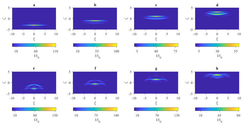
Figure 2: Distribution of the quantity $I/I_{0}=\left(\partial\Psi/\partial\tau\right)^{2}$ in an array of nanotubes at various instants of dimensionless time $\tau$ during the passage of the wave packet, which is the solution of Eq. (5): (a) $\tau=0$, (b) $\tau=2.0$, (c) $\tau=4.0$, (d) $\tau=6.0$, (e) $\tau=28.0$, (f) $\tau=30.0$, (g) $\tau=32.0$, (h) $\tau=34.0$.

The color scale is assigned to different values of the ratio $I/I_{0}$: the yellow areas correspond to the maximum values, and the dark-blue areas correspond to the minimum values. The horizontal and vertical axes of the graph represent the dimensionless coordinates $\xi=x\omega_{0}/c$ and $\zeta=z\omega_{0}/c$. Given the system parameter values selected above, the unit along the $\xi$- and $\zeta$-axes corresponds to the distance $\approx 4.2\times 10^{-4}$ cm. We note that here we give the distribution of the quantity $I/I_{0}$ in the $\xi O\zeta$–plane only, since the pattern of the distribution of the intensity of the field in the $\upsilon O\zeta$–plane is qualitatively similar.

We draw attention to the fact that in order to save computation time and to simplify the visual representation, we used a numerical scheme with periodic boundary conditions (see the details in our previous work [40]). For this reason, in Figure 2 (and also in Figure 3), the positions of the wave packet at the later instants (“e”– “h”) belong to the same spatial interval along the $\zeta$-axis that corresponds to the positions of the wave packet at the earlier time instants (“a”–“d”). It can be seen from Fig. 2 that the wave packet, having overcome a distance substantially exceeding its characteristic size along the direction of propagation (along the positive $\zeta$ direction), retains its individuality without undergoing a decay due to diffraction and dispersive spreading.

Figure 3 shows the evolution of the distribution profile of the electric component of the field $E_{x}$ (Eq. (10)) of a given wave packet and the intensity $I$ along the $\zeta$-axis passing through the point with coordinates $\xi=\xi_{0}$ and $\upsilon=\upsilon_{0}$, corresponding to the initial position of the “center of mass" of the pulse in the $\xi O\zeta$–plane at the same instants of dimensionless time $\tau$ as in Fig. 1. In this case, the center of mass of the pulse in the $\xi O\zeta$–plane is not displaced, i.e. according to the simulation results, $\xi_{\rm{pulse}}=\xi_{0}$ and $\upsilon_{\rm{pulse}}=\upsilon_{0}$.

It can be seen from Fig. 3 that during the observation time, $E_{x}$ is alternating between positive and negative values, that is, the electromagnetic pulse remains bipolar. The nature of the change in the configuration of the wave packet can be illustrated by the dependency of the scaled amplitude of the intensity $I_{\rm{max}}/I_{0}={\rm{max}}\left\{(\partial\Psi/\partial\tau)^{2}\right\}$ on the dimensionless time $\tau$. Figure 4 shows the time dependency of the quantity $I_{\rm{max}}/I_{0}$ for the same values of the system parameters as in Figs. 2 and 3.

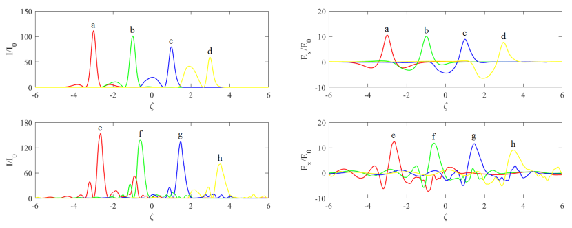
Figure 3: Distribution of the electric field strength $E_{x}/E_{0}$ and energy intensity $I/I_{0}$ on the $\zeta$-axis, in the course of the propagation of the electromagnetic pulse shown in Fig. 2, at various instants of dimensionless time: (a) $\tau=0$, (b) $\tau=2.0$, (c) $\tau=4.0$, (d) $\tau=6.0$, (e) $\tau=28.0$, (f) $\tau=30.0$, (g) $\tau=32.0$, (h) $\tau=34.0$.

As a result of numerical analysis, it is established that the wave packet preserves its individuality in the course of propagation, without undergoing significant spreading and damping; the electric field remains alternating over a time interval substantially exceeding the characteristic duration of the wave packet. Thus, this three-dimensional electromagnetic pulse has the properties of a nontopological soliton–breather, determined by the initial conditions (21) and (25). This circumstance allows one, in a certain sense, to consider a three-dimensional bipolar electromagnetic extremely short pulse propagating in an array of carbon nanotubes as being a soliton.

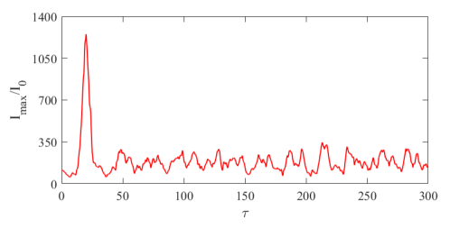
Figure 4: Dependency of the ratio $I_{\rm{max}}/I_{0}$ on the dimensionless time $\tau$ during the propagation of the electromagnetic pulse shown in Figs. 2 and 3. The dimensionless time $\tau=\omega_{0}t/\sqrt{\varepsilon}$ is plotted along the horizontal axis.

We note that the results presented here correspond to the situation in which the electromagnetic pulse propagates in an essentially nonlinear regime. We emphasize that in this case, the absolute values of the extrema of the projection of the dimensionless vector potential $\Psi$ on the nanotubes axis reach values of the order of unity (that is, the condition $|\sin\Psi|\ll 1$ is not satisfied in the general case) and, consequently, Eq. (5) cannot be linearized with the chosen values of the system parameters. From the physical point of view, this means that the response $j$ (electric current density) depends in an essentially nonlinear manner on the vector potential (and hence on the electric field strength) of the self-consistent field of the electromagnetic pulse (see formula (3) from our previous work [42]).

5.4 Reduced effective equation

5.4.1 3D generalization of the double sine-Gordon equation

As noted above, the coefficients $G_{r}$ (see Eq. (5)) decrease rapidly with increasing values of the index $r$. According to Eq. (4) from our previous work [42], and with the system parameters chosen above, we obtain the following values for the first five terms of the series $G_{r}$ (up to the second decimal place): $G_{1}\approx 0.91$, $G_{2}\approx 0.33$, $G_{3}\approx 0.18$, $G_{4}\approx 0.12$, and $G_{5}\approx 0.08$. Thus, in fact, the third term is already significantly smaller than the first one, which justifies the actual truncation to obtain the full effective equation, so that Eq. (6) is a satisfactory approximation of the original Eq. (5).

We have numerically solved the truncated effective Eq. (6) in the form of a three-dimensional generalized double sine-Gordon equation with initial conditions (20)–(25) on the dimensionless time interval ranging from $0$ to $\tau=300$. As a result, we established that the electromagnetic pulse propagates over a distance substantially exceeding its characteristic size, and does not undergo appreciable diffraction, transverse or dispersive longitudinal spreading. At the same time, the solution of the truncated effective Eq. (6) is a bipolar solitary electromagnetic wave with a “breathing" periodically repeating its shape profile. In other words, the evolution of the pulse field in model (6) is qualitatively similar to the behavior of the electromagnetic pulse in the model of the full effective Eq. (5). Thus, the evolution of the field of a three-dimensional electromagnetic pulse (with the same initial parameters) in an array of nanotubes is described by Eqs. (5) and  (6) in a qualitative way, but some quantitative differences in the values of the parameters of the steady-state solution in the form of a stably propagating bipolar solitary wave.

5.4.2 3D generalization of the sine-Gordon equation

We further simulated the propagation of the electromagnetic pulse within the framework of the model represented by the truncated effective Eq. (7), for the same values of the system parameters and with the same initial condition as before. It follows from the results of the calculations that the pulse of model (7) at long time scales also possesses the properties of a breather—a bipolar solitary wave—with a periodically changing “breathing" amplitude. Model (8) with the corrected coefficient $\sigma_{\Sigma}^{2}$ in front of the sine leads to a similar picture of the evolution of the pulse field: after the transient stage (a short-term increase in the degree of transverse field localization with a corresponding increase in amplitude), the pulse reaches a stable propagation mode, qualitatively similar to that in the framework of model (5).

5.5 Comparison of the pulse dynamics in the framework of complete and reduced models

To compare the behavior of the solutions obtained in the framework of different models represented by Eqs. (5)–(8), we analyze the time dependencies of the scaled amplitude of the maximum field intensity $I_{\rm{max}}/I_{0}$, and the ratio of the transverse half-width of the pulse $\lambda_{\perp}(\tau)$ to its initial value $\lambda_{\perp}(0)$ (see Eq. (19)).

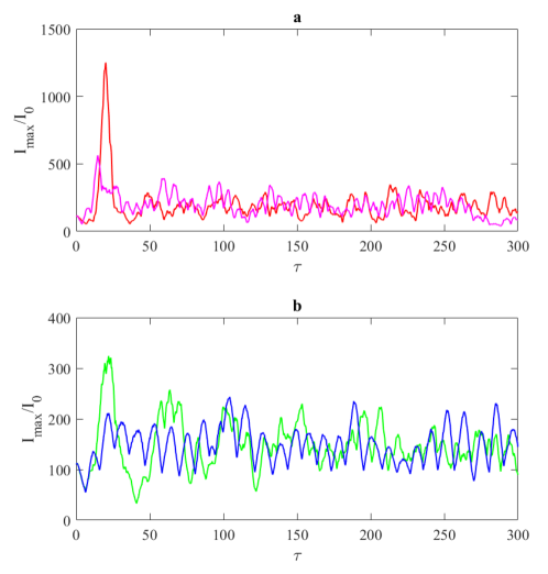
Figure 5: Dependency of the scaled maximum energy density of the pulse $I_{\rm{max}}/I_{0}$ on the dimensionless time $\tau$ along the $\zeta$-axis in the course of the electromagnetic pulse propagation in the full (Eq. (5)) and truncated models represented by Eqs. (6)–(8): (a) red – full effective Eq. (5); magenta – truncated model in the form of the three-dimensional generalization of the sine-Gordon Eq. (8) containing the coefficient $\sigma_{\Sigma}$; (b) green – truncated model in the form of the three-dimensional generalization of the double sine-Gordon Eq. (6); blue – truncated model in the form of the three-dimensional generalization of the sine-Gordon equation (7).

Figures 5 and 6 show, respectively, the time dependencies of the values of $I_{\rm{max}}/I_{0}$ and $\lambda_{\perp}/\lambda_{\perp}(0)$, obtained as a result of solving the effective Eqs. (5)–(8) at identical values of the system parameters and the same initial condition given by formulas (20)–(25). It can be seen from Fig. 5 that a noticeable difference in the behavior of the solution of Eq. (8), with the modified coefficient in front of the sine, from the behavior of the solutions within the remaining truncated models (6) and (7), is a more pronounced outgrowth of the field amplitude with the field focusing at the initial stage, which is similar to the behavior of the pulse within the framework of the model represented by the full effective Eq. (5). The amplitude and transverse width of the pulse reach values close to the initial values at the end of the transient process again, and the pulse dynamics reaches the mode corresponding to the stable propagation of a breather, which is the common result obtained within all the analyzed models (5)–(8). We also note that the truncated model in the form of Eq. (8) with the modified coefficient $\sigma_{\Sigma}$, in the most accurate manner (with respect to the full Eq. (5)) approximates the variations of the transverse width of the electromagnetic pulse due to diffraction. This conclusion follows from the analysis of the curves $\lambda_{\perp}(\tau)$ in Fig. 6.

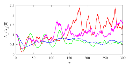
Figure 6: Dependency of the scaled transverse half-width of the pulse $\lambda_{\perp}/\lambda_{\perp}(0)$ on the dimensionless time $\tau$ during the propagation of the electromagnetic pulse under the same conditions as in Fig. 5: red – full effective Eq. (5); green – truncated model in the form of a three-dimensional generalization of the double sine-Gordon equation (6); blue and magenta – truncated model in the form of the three-dimensional generalization of the sine-Gordon equation (7) and (8), respectively.

Thus, comparing the numerical simulation results shown in Figs. 5 and 6, it can be seen that the model represented by the three-dimensional generalization of the sine-Gordon and the double sine-Gordon equations can adequately approximate the dynamics of the pulse at long time scales. We note that the truncated model in the form of a generalization of the sine-Gordon equation with the corrected coefficient calculated from the empirical formula (9), is the simplest and satisfactory model for the asymptotic analysis of the electromagnetic pulse dynamics at the long time scales.

6 Conclusions

Key results of this work may be summarized as follows:

• An effective equation (see Eq. (5)) is presented that determines the evolution of the electromagnetic field in an array of semiconductor carbon nanotubes, taking into account the limiting (three-dimensional) field localization.

• The evolution of an extremely short three-dimensional bipolar electromagnetic pulse in an array of nanotubes is analyzed by means of numerical simulations over a long time interval, which significantly exceeds the pulse durations, and still shorter than the relaxation time. The possibility of stable propagation of a bipolar electromagnetic pulse with limiting (three-dimensional) field localization in an array of nanotubes at large time scales is confirmed.

• The possibility of approximating the effective Eq. (5) by simpler models in the form of three-dimensional generalizations of the double sine-Gordon equation (6) and the sine-Gordon equation ((7)–(8)) is suggested and numerically verified.

• The dynamics of the pulse is compared in the framework of the models associated with the full effective Eq. (5) and the truncated effective Eqs. (6)–(8). It is established that the truncated effective equations are adequate models for the description of the dynamics of a three-dimensional electromagnetic pulse in an array of carbon nanotubes over long times.

Appendix

Possibilities of analytical consideration. Asymptotic analysis of the electromagnetic pulse dynamics

The applicability of Eqs. (6)–(8) proposed above opens the possibility for further progress in the analytical study of the problem of the dynamics of extremely short electromagnetic pulses in carbon nanotubes. Consider the illustration of an analytical approach to the asymptotic analysis of the field evolution over long times using the example of the model described by Eq. (7) (generalization to Eq. (6) is simple).

After re-normalization of time $\tau\to\sigma\tilde{\tau}$ and coordinates $\xi\to\sigma\tilde{\xi}$, $\upsilon\to\sigma\tilde{\upsilon}$, and $\zeta\to\sigma\tilde{\zeta}$, Eq. (7) can be considered as the Euler-Lagrange equation for the Lagrangian density,

$${\cal L}=\frac{1}{2}\left\{\left(\frac{\partial\Psi}{\partial\tilde{\tau}}\right)^{2}-\left(\frac{\partial\Psi}{\partial\tilde{\xi}}\right)^{2}-\left(\frac{\partial\Psi}{\partial\tilde{\upsilon}}\right)^{2}-\left(\frac{\partial\Psi}{\partial\tilde{\zeta}}\right)^{2}\right\}+\cos\Psi-1.$$ (27)

The change to the cylindrical coordinate system ($\tilde{\upsilon}=r\cos\theta$, $\tilde{\xi}=r\sin\theta$), as well as the assumption that the extremely short pulse preserves the cylindrical symmetry in the course of its propagation ($d\Psi/d\theta\rightarrow 0$) allows us to represent the Lagrangian density (27) in the form

$${\cal L}=\frac{1}{2}\left\{\left(\frac{\partial\Psi}{\partial\tilde{\tau}}\right)^{2}-\left(\frac{\partial\Psi}{\partial r}\right)^{2}-\left(\frac{\partial\Psi}{\partial\tilde{\zeta}}\right)^{2}\right\}+\cos\Psi-1.$$ (28)

Next, consider, according to the Whitham approach [59], a solution in the form of a $2\pi$–kink, in which the “fast" and “slow" variables are clearly distinguished:

$$\Psi=4\arctan\left\{\rho(\tilde{\tau}-\tilde{\zeta})-\Phi\right\},$$ (29)

where $\rho$ and $\Phi$ are the fast and slow variables, respectively. Passing further to the coordinates of the light cone for $\tilde{\tau}$ and $\tilde{\zeta}$, and also averaging over $(\tilde{\tau}-\tilde{\zeta})$, we obtain the corresponding Lagrangian density:

$${\cal L}=\rho\frac{\partial\Phi}{\partial Z}+\rho\left(\frac{\partial\Phi}{\partial r}\right)^{2}+\frac{1}{\rho}-\frac{\pi^{2}}{3\rho^{3}}\left(\frac{\partial\rho}{\partial r}\right)^{2},$$ (30)

where $Z=\tilde{\tau}+\tilde{\zeta}$.

The set of equations for the quantities $\rho$ and $\Phi$ corresponding to the Lagrangian density (30) has a hydrodynamic form [59]:

$$\frac{\partial\rho}{\partial Z} + \frac{\partial}{\partial r}\left(\rho\frac{\partial\varphi}{\partial r}\right)=0,$$

$$\frac{\partial\varphi}{\partial Z} + \frac{1}{2}\left(\frac{\partial\varphi}{\partial r}\right)^{2}-\frac{2}{\rho^{2}}=\frac{\pi^{2}}{6\rho^{3}}\left(\frac{\partial^{2}\rho}{\partial r^{2}}\right)-\frac{3}{2\rho}\left(\frac{\partial\rho}{\partial r}\right)^{2},$$ (31)

where the notation $\varphi=-2\Phi$ is introduced for convenience of presentation. An analogy with the hydrodynamics of an ideal fluid arises when the right-hand side of Eq. (31) is equated to zero. In this case, the quantity $\rho$ has the meaning of density, the quantity $\varphi$ corresponds to the potential of the velocity field, and the quantity $-2/\rho^{2}\equiv H(\rho)$ plays the role of enthalpy [60]. Considering the relationship between enthalpy and pressure $P$ in the form $H(\rho)=\int\rho^{-1}dP$, we consider the stability of our solution with respect to long-wavelength transverse perturbations of such a kind that the right-hand side of Eq. (31) can be neglected. In this case, taking into account the results from hydrodynamics, it is necessary to satisfy the condition $P>0$ for the stability of the solution. Thus, the hydrodynamic analogy for the model described by Eq. (7) allows one to establish the stability of its solutions in the form of kinks over arbitrary (long) time scales. Development and application of this analytical approach with respect to solitary waves of other types, including breathers, is also of interest, and we consider it as a subject for further research.

Funding

A. V. Zhukov and R. Bouffanais are financially supported by the SUTD-MIT International Design Centre (IDC). N. N. Rosanov acknowledges the support from the Russian Foundation for Basic Research, Grant 19-02-00312, and from the Foundation for the Support of Leading Universities of the Russian Federation (Grant 074-U01). M. B. Belonenko acknowledges support from the Russian Foundation for Fundamental Research.

Disclosures

The authors declare that there are no conflicts of interest related to this article.

References

- [1] Y. Segawa, H. Ito, and K. Itami, Nat. Rev. Mater. 1, 15002 (2016).
- [2] R. H. Baughman, A. A. Zakhidov, and W. A. de Heer, Science 297, 787 (2002).
- [3] A.V. Eletskii, Physics-Uspekhi 40 , 899 (1997).
- [4] M. B. Belonenko, S. Yu. Glazov, and N. E. Meshcheryakova, Bull. Russ. Acad. of Sci.: Physics 73, 1601 (2009).
- [5] A. V. Zhukov, R. Bouffanais, M. B. Belonenko, and E. G. Fedorov, Mod. Phys. Lett. B 27, 1350045 (2013).
- [6] M. B. Belonenko and E. G. Fedorov, Russ. Phys. J. 55, 83 (2012).
- [7] S. A. Akhmanov, V. A. Vysloukh, and A. S. Chirkin, Optics of Femtosecond Laser Pulses (American Institute of Physics, 1992).
- [8] Y. Yin, X. Ren, A. Chew, J. Li, Y. Wang, F. Zhuang, Y. Wu, and Z. Chang, Sci. Rep. 7, 11097 (2017).
- [9] S. Wandel, G. Xu, Y. Yin, and I. Jovanovic, J. Phys. B: At. Mol. Opt. Phys. 47, 234016 (2014).
- [10] D. D. Hudson, Opt. Fiber Technol. 20, 631 (2014).
- [11] A. M. Zheltikov, Phys. Usp. 50, 705 (2007).
- [12] A. Couairon, J. Beigert, C. P. Hauri, W. Kornelis, F. W. Helbing, U. Keller, and A. Mysyrowicz, J. Mod. Opt. 53, 75 (2006).
- [13] S. M. Foreman, D. J. Jones, and J. Ye, Opt. Lett. 28, 307 (2003).
- [14] J. A. Gruetzmacher and N. F. Scherer, Rev. Sci. Instr. 73, 2227 (2002).
- [15] E. Riedle, M. Beutter, S. Lochbrunner, J. Piel, S. Schenkl, S. Spörlein, and W. Zinth, Appl. Phys. B 71, 457 (2000).
- [16] E. R. Mueller, T. E. Wilson, and J. Waldman, Appl. Phys. Lett. 64, 3383 (1994).
- [17] S. V. Sazonov, Bull. Russ. Acad. Sci.: Physics 75, 157 (2011).
- [18] H. Leblond and D. Mihalache, Phys. Rep. 523, 61 (2013).
- [19] G. Mourou, S. Mironov, E. Khazanov, and A. Sergeev, Eur. Phys. J. Special Topics 223, 1181 (2014).
- [20] M. Kolesik and J. V. Moloney, Rep. Prog. Phys. 77, 016401 (2014).
- [21] D. J. Frantzeskakis, H. Leblond, and D. Mihalache, Rom. J. Phys. 59, 767 (2014).
- [22] B. A. Malomed, D. Mihalache, F. Wise, and L. Torner, J. Opt. B.: Quantum Semiclass. Opt. 7, R53 (2005).
- [23] D. Mihalache, Rom. J. Phys. 57, 352 (2012).
- [24] D. Mihalache, Rom. J. Phys. 59, 295 (2014).
- [25] A. Demircan, Sh. Amiranashvili, and G. Steinmeyer, Phys. Rev. Lett. 106, 163901 (2011).
- [26] Sh. Amiranashvili and A. Demircan, Phys. Rev. A 82, 013812 (2010).
- [27] I. Babushkin, A. Tajalli, H. Sayinc, U. Morgner, G. Steinmeyer, and A. Demircan, Light: Science & Applications 6, e16218 (2017).
- [28] A. V. Pakhomov, R. M. Arkhipov, I. V. Babushkin, M. V. Arkhipov, Yu. A. Tolmachev, and N. N. Rosanov, Phys. Rev. A 95, 013804 (2017).
- [29] M. V. Arkhipov, R. M. Arkhipov, A. V. Pakhomov, I. V. Babushkin, A. Demircan, U. Morgner, and N. N. Rosanov, Opt. Lett. 42, 2189 (2017).
- [30] D. Mihalache, Rom. Rep. Phys. 69, 403 (2017).
- [31] S. V. Sazonov, Rom. Rep. Phys. 70, 401 (2018).
- [32] M. B. Belonenko, E. V. Demushkina, and N. G. Lebedev, J. Russ. Laser Res. 27, 457 (2006).
- [33] M. B. Belonenko, N. G. Lebedev, E. N. Nelidina, Phys. Wave Phenom. 19, 39 (2011).
- [34] E. G. Fedorov, A. V. Zhukov, M. B. Belonenko, and T. F. George, Eur. Phys. J. D 66, 219 (2012).
- [35] H. Leblond and D. Mihalache, Phys. Rev. A 86, 043832 (2012).
- [36] E. G. Fedorov, A. V. Pak, and M. B. Belonenko, Phys. Sol. State 56, 2112 (2014).
- [37] A. V. Zhukov, R. Bouffanais, E. G. Fedorov, and M. B. Belonenko, J. Appl. Phys. 115, 203109 (2014).
- [38] E. G. Fedorov, N. N. Konobeeva, and M. B. Belonenko, Rus. J. Phys. Chem. B 8, 409 (2014).
- [39] M. B. Belonenko and E. G. Fedorov, Phys. Sol. State 55, 1333 (2013).
- [40] A. V. Zhukov, R. Bouffanais, H. Leblond, D. Mihalache, E. G. Fedorov, and M. B. Belonenko, Eur. Phys. J. D 69, 242 (2015).
- [41] A. V. Zhukov, R. Bouffanais, E. G. Fedorov, and M. B. Belonenko, J. Appl. Phys. 114, 143106 (2013).
- [42] A. V. Zhukov, R. Bouffanais, B. A. Malomed, H. Leblond, D. Mihalache, E. G. Fedorov, N. N. Rosanov, and M. B. Belonenko, Phys. Rev. A 94, 053823 (2016).
- [43] E. G. Fedorov, A. V. Zhukov, R. Bouffanais, A. P. Timashkov, B. A. Malomed, H. Leblond, D. Mihalache, N. N. Rosanov, and M. B. Belonenko, Phys. Rev. A 97, 043814 (2018).
- [44] M. B. Belonenko, N. G. Lebedev, and E. N. Nelidina, Russ. Phys. J. 53, 1118 (2011).
- [45] L. D. Landau, E. M. Lifshitz, and L. P. Pitaevskii, Electrodynamics of Continuous Media, 2nd Ed. (Elsevier, Oxford, 2004).
- [46] L. D. Landau and E. M. Lifshitz, The Classical Theory of Fields, 4th Ed. (Butterworth-Heinemann, Oxford, 2000).
- [47] E. M. Epshtein, Fiz. Tverd. Tela 19, 3456 (1976).
- [48] E. M. Epshtein, Fiz. Tech. Polupr. 14, 2422 (1980) [Sov. Phys. Semiconductors 14, 1438 (1980)].
- [49] F. G. Bass, A. A. Bulgakov, and A. P. Tetervov, High Frequency Properties of Semiconductors with Superlattices (Nauka, Moscow, 1989).
- [50] Yu. S. Kivshar and B. A. Malomed, Rev. Mod. Phys. 61, 763 (1989).
- [51] D. Mihalache, D. Mazilu, L.-C. Crasovan, I. Towers, A. V. Buryak, B. A. Malomed, L. Torner, J. P. Torres, and F. Lederer, Phys. Rev. Lett. 88, 073902 (2002).
- [52] J.-C. Diels and W. Rudolph, Ultrashort Laser Pulse Phenomena. Fundamentals, Techniques, and Applications on a Femtosecond Scale (Elsevier, 2006).
- [53] C. Rulliére, Ed., Femtosecond Laser Pulses: Principles and Experiments (Springer-Verlag, Berlin, 1998).
- [54] A. N. Pikhtin, Optical and Quantum Electronics (High School Publishers, Moscow, 2001).
- [55] A.M. Goncharenko, Gaussian Light Beams (Nauka i tehnika, Minsk, 1976).
- [56] N. N. Kalinkin, Numerical Methods (Nauka, Moscow, 1978).
- [57] S. E. Koonin, Computational Physics : Fortran Version ( Ingram Publisher Services, Boulder, Colorado, 1998).
- [58] J. W. Thomas, Numerical Partial Differential Equations – Finite Difference Methods (Springer-Verlag, New York, 1995).
- [59] G. B. Witham, Linear and Nonlinear Waves, (John Willey & Sons, 1974).
- [60] L. D. Landau and E. M. Lifshitz, Fluid Mechanics, 2nd Ed. (Elsevier, 1987).