Statistical Inferences of Linear Forms for Noisy Matrix Completion^∗

Abstract

We introduce a flexible framework for making inferences about general linear forms of a large matrix based on noisy observations of a subset of its entries. In particular, under mild regularity conditions, we develop a universal procedure to construct asymptotically normal estimators of its linear forms through double-sample debiasing and low-rank projection whenever an entry-wise consistent estimator of the matrix is available. These estimators allow us to subsequently construct confidence intervals for and test hypotheses about the linear forms. Our proposal was motivated by a careful perturbation analysis of the empirical singular spaces under the noisy matrix completion model which might be of independent interest. The practical merits of our proposed inference procedure are demonstrated on both simulated and real-world data examples.

1 Introduction

Noisy matrix completion (NMC) refers to the reconstruction of a low rank matrix $M\in\mathbb{R}^{d_{1}\times d_{2}}$ after observing a small subset of $M$’s entries with random noise. Problems of this nature arise naturally in various applications. For the sake of generality, we shall cast it in the framework of trace regression where each observation is a random pair $(X,Y)$ with $X\in\mathbb{R}^{d_{1}\times d_{2}}$ and $Y\in\mathbb{R}$. The random matrix $X$ is sampled uniformly from the orthonormal basis $\mathfrak{E}=\{e_{j_{1}}e_{j_{2}}^{\mathsf{T}}:j_{1}\in[d_{1}],j_{2}\in[d_{2}]\}$ where $[d]=\{1,\cdots,d\}$ and $\{e_{j_{1}}\}_{j_{1}\in[d_{1}]}$ and $\{e_{j_{2}}\}_{j_{2}\in[d_{2}]}$ are the canonical basis vectors in $\mathbb{R}^{d_{1}}$ and $\mathbb{R}^{d_{2}}$, respectively. It is worth pointing out that, while we shall focus on the canonical basis in this work, our framework can be easily extended to general product basis where $\{e_{j_{1}}\}_{j_{1}\in[d_{1}]}$ and $\{e_{j_{2}}\}_{j_{2}\in[d_{2}]}$ are arbitrary orthonormal basis in $\mathbb{R}^{d_{1}}$ and $\mathbb{R}^{d_{2}}$, respectively. Without loss of generality, we shall assume that $d_{1}\geq d_{2}$ and denote $\alpha_{d}=d_{1}/d_{2}$ the aspect ratio of $M$. The response variable $Y$ is related to $X$ via

$$Y=\langle M,X\rangle+\xi$$ (1.1)

where $\langle M,X\rangle=\operatorname{tr}(M^{\mathsf{T}}X)$, and the independent measurement error $\xi$ is assumed to be a centered sub-Gaussian random variable. Our goal is to infer $M$ from $n$ i.i.d. copies $\{(X_{i},Y_{i})\}_{i=1}^{n}$ obeying (1.1) when, in particular, $M$ is of (approximately) low rank and $n$ is much smaller than $d_{1}d_{2}$.

In the absence of measurement error (e.g., $\xi=0$), Candès and Recht (2009) first discovered that exact matrix completion can be solved efficiently by relaxing the non-convex and non-smooth rank constraint of a matrix to its nuclear norm. Following the pioneering work, nuclear-norm penalized least squares estimators (Negahban and Wainwright, 2011; Rohde and Tsybakov, 2011; Cai et al., 2010; Cai and Zhou, 2016; Candès and Tao, 2009; Candes and Plan, 2010; Gross, 2011) and numerous other variants (Koltchinskii et al., 2011; Klopp, 2014; Liu, 2011; Recht et al., 2010; Sun and Zhang, 2012; Cai and Zhang, 2015; Gao et al., 2016) have been studied. It is now understood, from these developments, that even when the observations are contaminated with noise, statistically optimal convergence rates are attainable by efficiently computable convex methods. For instance, Koltchinskii et al. (2011) proved that a modified matrix LASSO estimator, denoted by $\widehat{M}^{\scriptscriptstyle\sf KLT}$, achieves the convergence rate:

$$\|\widehat{M}^{\scriptscriptstyle\sf KLT}-M\|_{\scriptscriptstyle\sf F}^{2}=O_{P}\Big{(}(\sigma_{\xi}+\|M\|_{\scriptscriptstyle\sf max})^{2}\cdot\frac{rd_{1}^{2}d_{2}\log d_{1}}{n}\Big{)}$$ (1.2)

as long as $n\gg d_{1}\log d_{1}$ where $r$ is the rank of $M$ and $\sigma_{\xi}^{2}$ is the variance of $\xi$. Here, $\|\cdot\|_{\scriptscriptstyle\sf F}$ denotes the matrix Frobenius norm and $\|\cdot\|_{\scriptscriptstyle\sf max}$ denotes the max-norm defined as $\|A\|_{\scriptscriptstyle\sf max}=\max_{j_{1}\in[d_{1}],j_{2}\in[d_{2}]}|A(j_{1},j_{2})|$. It is worth noting that (1.2) was established without additional assumptions on $M$. As a result, the rate given on the righthand side of (1.2) depends on $\|M\|_{\scriptscriptstyle\sf max}$ and does not vanish even when $\sigma_{\xi}=0$.

In addition to convex methods, non-convex approaches such as those based on matrix-factorization have also been developed. For instance, Keshavan et al. (2010b) proposed a non-convex estimator based on the thin SVD, denoted by $\widehat{M}^{\scriptscriptstyle\sf KMO}$, and show that

$$\|\widehat{M}^{\scriptscriptstyle\sf KMO}-M\|_{\scriptscriptstyle\sf F}^{2}=O_{P}\Big{(}\sigma_{\xi}^{2}\cdot\frac{rd_{1}^{2}d_{2}\log d_{1}}{n}\Big{)}$$ (1.3)

assuming that $n\gg rd_{1}(r+\log d_{1})$ and $M$ satisfies the so-called incoherent condition. See also, e.g., Zhao et al. (2015); Chen and Wainwright (2015); Cai et al. (2016b) and references therein. The rate (1.3) is optimal up to the logarithmic factors, see, e.g., Koltchinskii et al. (2011) and Ma and Wu (2015), for a comparable minimax lower bound. More recently, an alternative scheme of matrix factorization attracted much attention. See, e.g., Wang et al. (2016); Ge et al. (2016); Zheng and Lafferty (2016); Chen et al. (2019c, b); Ma et al. (2017); Chen et al. (2019a). In particular, Ma et al. (2017) showed this approach yields an estimator, denoted by $\widehat{M}^{\scriptscriptstyle\sf MWC}$, that is statistically optimal not only in matrix Frobenius norm but also in entry-wise max-norm, i.e.,

$$\|\widehat{M}^{\scriptscriptstyle\sf MWC}-M\|_{\scriptscriptstyle\sf max}^{2}=O_{P}\Big{(}\sigma_{\xi}^{2}\cdot\frac{rd_{1}\log d_{1}}{n}\Big{)}$$ (1.4)

provided that $n\gg r^{3}d_{1}\log^{3}d_{1}$.

While there is a rich literature on statistical estimation for NMC, results about its statistical inferences are relatively scarce. In Carpentier et al. (2015), a debiasing procedure, based on sample splitting, was proposed for the nuclear norm penalized least squares estimator which enables constructing confidence region for $M$ with respect to matrix Frobenius norm when $n\gg rd_{1}\log d_{1}$. Their technique, however, cannot be directly used to make inferences about individual entries or linear forms as confidence regions for $M$ with respect to matrix Frobenius norm can be too wide for such purposes. To this end, Carpentier et al. (2018) proposed another procedure to construct entrywise confidence intervals. However their procedure requires that the design, namely the underlying distribution of $X$ satisfy the so-called restricted isometry property which is violated when $X$ is sampled uniformly from $\mathfrak{E}$. Another proposal introduced by Cai et al. (2016a) can be used to construct confidence intervals for $M$’s entries. However, it requires that the sample size $n\gg d_{1}d_{2}$ which is significantly larger than the optimal sample size requirement for estimation. In addition, during the preparation of the current work, Chen et al. (2019c) announced a different approach to constructing confidence intervals for the entries of $M$.

The present article aims to further expand this line of research by introducing a flexible framework for constructing confidence intervals and testing hypotheses about general linear forms of $M$, with its entries as special cases, under optimal sample size requirement. In a nutshell, we develop a procedure that, given any entry-wise consistent estimator $\widehat{M}^{\scriptscriptstyle\sf init}$ in that $\|\widehat{M}^{\scriptscriptstyle\sf init}-M\|_{\scriptscriptstyle\sf max}=o_{P}(\sigma_{\xi})$, can yield valid statistical inferences for $m_{T}:=\operatorname{tr}(M^{\mathsf{T}}T)$ under mild regularity conditions. More specifically, we show that, through double-sample debiasing and spectral projection, we can obtain from the initial estimator a new one, denoted by $\widehat{M}$, so that

$$\frac{\operatorname{tr}(\widehat{M}^{\mathsf{T}}T)-\operatorname{tr}(M^{\mathsf{T}}T)}{\sigma_{\xi}(\|U^{\mathsf{T}}T\|_{\scriptscriptstyle\sf F}^{2}+\|TV\|_{\scriptscriptstyle\sf F}^{2})^{1/2}\sqrt{d_{1}d_{2}/n}}\overset{{\rm d}}{\longrightarrow}{\cal N}(0,1),$$ (1.5)

provided that

$$\|U^{\mathsf{T}}T \|_{\scriptscriptstyle\sf F}+\|TV\|_{\scriptscriptstyle\sf F}\gg\|T\|_{\ell_{1}}\sqrt{\frac{r}{d_{1}}}\cdot\max\bigg{\{}\sqrt{\frac{r\log d_{1}}{d_{2}}},\ \frac{\sigma_{\xi}}{\lambda_{r}}\sqrt{\frac{\alpha_{d}rd_{1}^{2}d_{2}\log^{2}d_{1}}{n}}\bigg{\}}$$

where $U,V$ are $M$’s left and right singular vectors and $\lambda_{r}$ is its $r$-th singular value, and $\|\cdot\|_{\ell_{1}}$ stands for the vectorized $\ell_{1}$ norm. We not only show that (1.5) holds under optimal sample size (independent of $T$) but also derive its non-asymptotic convergence rate explicitly. Note that condition for $\|U^{\mathsf{T}}T\|_{\scriptscriptstyle\sf F}+\|TV\|_{\scriptscriptstyle\sf F}$ in a certain sense is necessary to avoid non-regular asymptotic behavior when $\|U^{\mathsf{T}}T\|_{\scriptscriptstyle\sf F}+\|TV\|_{\scriptscriptstyle\sf F}=0$. Moreover, we show that under similar conditions, (1.5) continues to hold when we replace $\sigma_{\xi}$, $\|U^{\mathsf{T}}T\|_{\scriptscriptstyle\sf F}$ and $\|TV\|_{\scriptscriptstyle\sf F}$ by suitable estimates, denoted by $\widehat{\sigma}_{\xi}$, $\|\widehat{U}^{\mathsf{T}}T\|_{\scriptscriptstyle\sf F}$ and $\|T\widehat{V}\|_{\scriptscriptstyle\sf F}$ respectively:

$$\frac{\operatorname{tr}(\widehat{M}^{\mathsf{T}}T)-\operatorname{tr}(M^{\mathsf{T}}T)}{\widehat{\sigma}_{\xi}(\|\widehat{U}^{\mathsf{T}}T\|_{\scriptscriptstyle\sf F}^{2}+\|T\widehat{V}\|_{\scriptscriptstyle\sf F}^{2})^{1/2}\sqrt{d_{1}d_{2}/n}}\overset{{\rm d}}{\longrightarrow}{\cal N}(0,1).$$ (1.6)

The statistic on the lefthand side is now readily applicable for making inferences about the linear form $\operatorname{tr}(M^{\mathsf{T}}T)$.

Our proposal greatly generalizes the scope of earlier works on inferences for entries of $M$ in several crucial aspects. Firstly, unlike earlier approaches that focus on a specific estimator of $M$, our procedure can be applied to any entry-wise consistent estimator. This not only brings potential practical benefits but also helps us better understand the fundamental differences between estimation and testing in the context of NMC. For instance, our results suggest that, perhaps surprisingly, when it comes to make valid inferences with optimal sample sizes, the rate of convergence of the initial estimate is irrelevant as long as it is consistent; therefore a suboptimal estimator may be used for making optimal inferences.

Secondly, our approach can be applied in general when $T$ is sparse, and depending on its alignment with the singular spaces of $M$, even to cases where it is dense and $\|T\|_{\ell_{1}}^{2}/\|T\|_{\scriptscriptstyle\sf F}^{2}$ is of the order $O(d_{2})$. Entry-wise inferences correspond to the special case when $T$ takes the form $e_{i}e_{j}^{\mathsf{T}}$. Extensions to more general linear forms could prove useful in many applications. For example, in recommender systems, it may be of interest to decide between items $j_{1}$ and $j_{2}$ which should we recommend to user $i$. This can obviously be formulated as a testing problem:

$$H_{0}:M(i,j_{1})=M(i,j_{2})\quad{\rm v.s.}\quad H_{1}:M(i,j_{1})>M(i,j_{2}),$$ (1.7)

which can be easily solved within our framework by taking $T=e_{i}e_{j_{1}}^{\mathsf{T}}-e_{i}e_{j_{2}}^{\mathsf{T}}$. More generally, if the target is a group of users ${\cal G}\subset[d_{1}]$, we might take a linear form $T=\sum_{i\in{\cal G}}e_{i}(e_{j_{1}}-e_{j_{2}})^{\mathsf{T}}$. At a technical level, inferences about general linear forms as opposed to entries of $M$ present nontrivial challenges because of the complex dependence structure among the estimated entries. As our theoretical analysis shows, the variance of the plug-in estimator for the linear form depends on the alignment of the linear form with respect to the singular space of $M$ rather than the sparsity of the linear form.

An essential part of our technical development is the characterization of the distribution of the empirical singular vectors for NMC where we take advantage of the recently developed spectral representation for empirical singular vectors. Similar tools have been used earlier to derive confidence regions for singular subspaces with respect to $\ell_{2}$-norm for low-rank matrix regression (LMR) when the linear measurement matrix $X$s are Gaussian (Xia, 2019a), and the planted low rank matrix (PLM) model where every entry of $M$ is observed with i.i.d. Gaussian noise (Xia, 2019b). In both cases, Gaussian assumption plays a critical role and furthermore, it was observed that first order approximation may lead to suboptimal performances. In absence of the Gaussian assumption, the treatment of NMC is technically more challenging and requires us to derive sharp bounds for the $(2,\max)$-norm for the higher order perturbation terms. Interestingly, it turns out that, unlike LMR or PLM, a first order approximation actually suffices for NMC.

Even though our framework applies to any max-norm consistent matrix estimator, for concreteness, we introduce a novel rotation calibrated gradient descent algorithm on Grassmannians that yields such an initial estimator. The rotation calibration promotes fast convergence on Grassmannians so that constant stepsize can be selected to guarantee geometric convergence. We note that existing results on max-norm convergence rates are established for sampling without replacement (Ma et al., 2017). It is plausible that (1.4) may continue to hold under our assumption of independent sampling given the close connection between the two sampling schemes, but an actual proof is likely much more involved and therefore we opted for the proposed alternative for illustration as it is more amenable for analysis.

The rest of our paper is organized as follows. In next section, we present a general framework for estimating $m_{T}=\operatorname{tr}(M^{\mathsf{T}}T)$ given an initial estimator through double-sample-debiasing and spectral projection. In Section 3, we establish the asymptotic normality of the estimate obtained. In Section 4, we propose data-driven estimates for the noise variance and the true singular vectors, based on which confidence intervals of $m_{T}$ are constructed. In Section 5, we introduce a rotation calibrated gradient descent algorithm on Grassmannians, which, under mild conditions, provides the initial estimator $\widehat{M}^{\scriptscriptstyle\sf init}$ so that $\|\widehat{M}^{\scriptscriptstyle\sf init}-M\|_{\scriptscriptstyle\sf max}=o_{P}(\sigma_{\xi})$. Numerical experiments on both synthetic and real world datasets presented in Section 6 further demonstrate the merits of the proposed methodology. All proofs are presented in the online supplement.

2 Estimating Linear Forms

We are interested in making inferences about $m_{T}=\operatorname{tr}(M^{\mathsf{T}}T)$ for a given $T$ based on observations $\mathfrak{D}=\{(X_{i},Y_{i}):1\leq i\leq n\}$ satisfying model (1.1), assuming that $M$ has low rank. To this end, we first need to construct an appropriate estimate of $m_{T}$ which we shall do in this section.

Without loss of generality, we assume $n$ is an even number with $n=2n_{0}$, and split $\mathfrak{D}$ into two sub-samples:

$$\mathfrak{D}_{1}=\big{\{}(X_{i},Y_{i})\big{\}}_{i=1}^{n_{0}}\quad{\rm and}\quad\mathfrak{D}_{2}=\big{\{}(X_{i},Y_{i})\big{\}}_{i=n_{0}+1}^{n}.$$

In what follows, we shall denote $M$’s thin singular value decomposition (SVD) by $M=U\Lambda V^{\mathsf{T}}$ where $U\in\mathbb{O}^{d_{1}\times r},V\in\mathbb{O}^{d_{2}\times r}$ and $\Lambda={\rm diag}(\lambda_{1},\cdots,\lambda_{r})$ represent $M$’s singular vectors and singular values, respectively. The Stiefel manifold $\mathbb{O}^{d\times r}$ is defined as $\mathbb{O}^{d\times r}:=\big{\{}A\in\mathbb{R}^{d\times r}:A^{\mathsf{T}}A=I\big{\}}.$ We arrange $M$’s positive singular values non-increasingly, i.e., $\lambda_{1}\geq\cdots\geq\lambda_{r}>0$.

Assuming the availability of an initial estimator, our procedure consists of four steps as follows:

• Step 1 (Initialization): By utilizing the first and second data sub-sample $\mathfrak{D}_{1},\mathfrak{D}_{2}$ separately, we apply the initial estimating procedure on noisy matrix completion to yield initial (biased in general) estimates $\widehat{M}_{1}^{\scriptscriptstyle\sf init}$ and $\widehat{M}_{2}^{\scriptscriptstyle\sf init}$, respectively.

• Step 2 (Debiasing): Using the second data sub-sample $\mathfrak{D}_{2}$, we debias $\widehat{M}_{1}^{\scriptscriptstyle\sf init}$:

  $$\widehat{M}_{1}^{\scriptscriptstyle\sf unbs}=\widehat{M}_{1}^{\scriptscriptstyle\sf init}+\frac{d_{1}d_{2}}{n_{0}}\sum_{i=n_{0}+1}^{n}\big{(}Y_{i}-\langle\widehat{M}_{1}^{\scriptscriptstyle\sf init},X_{i}\rangle\big{)}X_{i}.$$

  Similarly, we use the first data sub-sample $\mathfrak{D_{1}}$ to debias $\widehat{M}_{2}^{\scriptscriptstyle\sf init}$ and obtain

  $$\widehat{M}_{2}^{\scriptscriptstyle\sf unbs}=\widehat{M}_{2}^{\scriptscriptstyle\sf init}+\frac{d_{1}d_{2}}{n_{0}}\sum_{i=1}^{n_{0}}\big{(}Y_{i}-\langle\widehat{M}_{2}^{\scriptscriptstyle\sf init},X_{i}\rangle\big{)}X_{i}.$$

• Step 3 (Projection): Compute the top-$r$ left and right singular vectors of $\widehat{M}_{1}^{\scriptscriptstyle\sf unbs}$, denoted by $\widehat{U}_{1}$ and $\widehat{V}_{1}$. Similarly, compute the top-$r$ left and right singular vectors of $\widehat{M}_{2}^{\scriptscriptstyle\sf unbs}$, denoted by $\widehat{U}_{2}$ and $\widehat{V}_{2}$. Then, we calculate the (averaged) projection estimate

  $$\widehat{M}=\frac{1}{2}\widehat{U}_{1}\widehat{U}_{1}^{\mathsf{T}}\widehat{M}_{1}^{\scriptscriptstyle\sf unbs}\widehat{V}_{1}\widehat{V}_{1}^{\mathsf{T}}+\frac{1}{2}\widehat{U}_{2}\widehat{U}_{2}^{\mathsf{T}}\widehat{M}_{2}^{\scriptscriptstyle\sf unbs}\widehat{V}_{2}\widehat{V}_{2}^{\mathsf{T}}.$$

• Step 4 (Plug-in): Finally, we estimate $m_{T}$ by $\widehat{m}_{T}=\operatorname{tr}(\widehat{M}^{\mathsf{T}}T)$.

We now discuss each of the steps in further details.

Initialization.

Apparently, our final estimate depends on the initial estimates $\widehat{M}_{1}^{\scriptscriptstyle\sf init},\widehat{M}_{2}^{\scriptscriptstyle\sf init}$. However, as we shall show in the next section, such dependence is fairly weak and the resulting estimate $\widehat{m}_{T}$ is asymptotically equivalent as long as the estimation error of $\widehat{M}_{1}^{\scriptscriptstyle\sf init}$ and $\widehat{M}_{2}^{\scriptscriptstyle\sf init}$, in terms of max-norm, is of a smaller order than $\sigma_{\xi}$. More specifically, we shall assume that

Assumption 1.

There exists a sequence $\gamma_{n,d_{1},d_{2}}\to 0$ as $n,d_{1},d_{2}\to\infty$ so that with probability at least $1-d_{1}^{-2}$,

$$\|\widehat{M}_{1}^{\scriptscriptstyle\sf init}-M\|_{\scriptscriptstyle\sf max}+\|\widehat{M}_{2}^{\scriptscriptstyle\sf init}-M\|_{\scriptscriptstyle\sf max}\leq C\gamma_{n,d_{1},d_{2}}\cdot\sigma_{\xi}$$ (2.1)

for an absolute constant $C>0$.

In particular, bounds similar to (2.1) have recently been established by Ma et al. (2017); Chen et al. (2019c). See eq. (1.4). Assumption 1 was motivated by their results. However, as noted earlier, (1.4) was obtained under sampling without replacement and for positively semi-definite matrices. While it is plausible that it also holds under independent sampling as considered here, an actual proof is lacking at this point. For concreteness, we shall present a simple algorithm in Section 5 capable of producing an initial estimate that satisfies Assumption 1.

Debiasing.

The initial estimate is only assumed to be consistent. It may not necessarily be unbiased or optimal. To ensure good quality of our final estimate $\widehat{m}_{T}$, it is important that we first debias it which allows for sharp spectral perturbation analysis. Debiasing is an essential technique in statistical inferences of high-dimensional sparse linear regression (see, e.g., Zhang and Zhang, 2014; Javanmard and Montanari, 2014; Van de Geer et al., 2014; cai2017confidence) and low-rank matrix regression (see, e.g., Cai et al., 2016a; Carpentier and Kim, 2018; Carpentier et al., 2018; Xia, 2019a). Oftentimes, debiasing is done in absence of the knowledge of $\mathbb{E}{\rm vec}(X){\rm vec}(X)^{\top}$ and a crucial step is to construct an appropriate decorrelating matrix. In our setting, it is clear that $\mathbb{E}{\rm vec}(X){\rm vec}(X)^{\top}=(d_{1}d_{2})^{-1}I_{d_{1}d_{2}}$. This allows for a much simplified treatment via sample splitting, in the same spirit as earlier works including Carpentier et al. (2015); Xia (2019a), among others. The particular double-sample-splitting technique we employ was first proposed by Chernozhukov et al. (2018) and avoids the loss of statistical efficiency associated with the sample splitting. It is worth noting that if the entries are not sampled uniformly, the debiasing procedure needs to be calibrated accordingly.

In addition to reducing possible bias of the initial estimate, the sample splitting also enables us to extend the recently developed spectral representation for empirical singular vectors under Gaussian assumptions to general sub-Gaussian distributions.

Spectral Projection.

Since $M$ have low rank, it is natural to apply spectral truncation to a matrix estimate to yield an improved estimate. To this end, we project $\widehat{M}_{1}^{\scriptscriptstyle\sf unbs}$ and $\widehat{M}_{2}^{\scriptscriptstyle\sf unbs}$ to their respective leading singular subspaces. Note that, while $\widehat{M}_{1}^{\scriptscriptstyle\sf unbs},\widehat{M}_{2}^{\scriptscriptstyle\sf unbs}$ are unbiased, their empirical singular vectors $\widehat{U}_{1},\widehat{U}_{2},\widehat{V}_{1}$ and $\widehat{V}_{2}$ are typically not. The spectral projection serves the purpose of reducing entry-wise variances at the cost of negligible biases.

It is worth noting that the estimate $\widehat{M}$ may not be of rank $r$. If an exact rank-$r$ estimator is desired, it suffices to obtain the best rank-$r$ approximation of $\widehat{M}$ via singular value decomposition and all our development remains valid under such a modification. In general, getting the initial estimates is the most computational expensive step as the other steps involving fairly standard operation without incurring any challenging optimization. This is noteworthy because it suggests that as long as we can compute a good estimate, it does not cost much more computationally to make inferences.

3 Asymptotic Normality of $\widehat{m}_{T}$

We now show the estimate $\widehat{m}_{T}$ we derived in the previous section is indeed suitable for inferences about $m_{T}$ by establishing its asymptotic normality.

3.1 General results

For brevity, let $e_{j}$ denote the $j$-th canonical basis in $\mathbb{R}^{d}$ where $d$ might be $d_{1}$ or $d_{2}$ or $d_{1}+d_{2}$ at different appearances. With slight abuse of notation, denote by $\|\cdot\|$ the matrix operator norm or vector $\ell_{2}$-norm depending on the dimension of its argument. Denote the condition number of $M$ by

$$\kappa(M)=\lambda_{1}(M)/\lambda_{r}(M)=\lambda_{1}/\lambda_{r}.$$ (3.1)

As is conventional in the literature, we shall assume implicitly that rank $r$ is known with $r\ll d_{2}$ and $M$ is well-conditioned so that $\kappa(M)\leq\kappa_{0}$. In practice, $r$ is usually not known in advance and needs to be estimated from the data. Our experience with numerical experiments such as those reported in Section 6 suggests that our procedure is generally robust to reasonable estimate of $r$. Although a more rigorous justification of such a phenomenon has thus far eluded us, these promising empirical observations nonetheless indicate a more careful future investigation is warranted.

In addition, we shall assume that $U$ and $V$ are incoherent, a standard condition for matrix completion.

Assumption 2.

Let $\|U\|_{\scriptscriptstyle\sf 2,max}=\max_{j\in[d_{1}]}\|e_{j}^{\mathsf{T}}U\|$ and there exists $\mu_{\scriptscriptstyle\sf max}>0$ so that

$$\max\Big{\{}\sqrt{\frac{d_{1}}{r}}\|U\|_{\scriptscriptstyle\sf 2,max},\sqrt{\frac{d_{2}}{r}}\|V\|_{\scriptscriptstyle\sf 2,max}\Big{\}}\leq\mu_{\scriptscriptstyle\sf max}.$$

We also assume that the noise $\xi$ is independent with $X$ and sub-Gaussian such that

Assumption 3.

The noise $\xi$ is independent with $X$ and

$$\mathbb{E}\xi=0,\quad\mathbb{E}\xi^{2}=\sigma_{\xi}^{2},\quad{\rm and}\quad\mathbb{E}e^{s\xi}\leq e^{s^{2}\sigma_{\xi}^{2}},\ \forall s\in\mathbb{R}$$ (3.2)

Let $\alpha_{d}=d_{1}/d_{2}$. There exists a large enough absolute constant $C_{1}>0$ so that

$$\lambda_{r}\geq C_{1}\mu_{\scriptscriptstyle\sf max}\kappa_{0}^{2}\sigma_{\xi}\sqrt{\frac{\alpha_{d}rd_{1}^{2}d_{2}\log^{2}d_{1}}{n}}.$$ (3.3)

The SNR condition (3.3) is optimal up to the logarithmic factors if $\alpha_{d},\mu_{\scriptscriptstyle\sf max},\kappa_{0}=O(1)$. Indeed, the consistent estimation of singular subspaces requires $\lambda_{r}\gg\sigma_{\xi}\sqrt{rd_{1}^{2}d_{2}/n}$. This condition is common for non-convex methods of NMC. However, when $\alpha_{d}\gg 1$, i.e., $M$ is highly rectangular, condition (3.3) is significantly stronger than the optimal SNR condition even if $\mu_{\scriptscriptstyle\sf max},\kappa_{0}=O(1)$. It is unclear to us whether this sub-optimality is due to technical issues or reflection of more fundamental differences between statistical estimation and inference.

To avoid the nonregular asymptotics, we focus on the case when $T$ does not lie entirely in the null space of $M$. More specifically, we assume that

Assumption 4.

There exists a constant $\alpha_{T}>0$ such that

$$\|U^{\mathsf{T}}T\|_{\scriptscriptstyle\sf F}\geq\alpha_{T}\|T\|_{\scriptscriptstyle\sf F}\cdot\sqrt{\frac{r}{d_{1}}}\quad{\rm or}\quad\|TV\|_{\rm F}\geq\alpha_{T}\|T\|_{\scriptscriptstyle\sf F}\cdot\sqrt{\frac{r}{d_{2}}}.$$

The alignment parameter $\alpha_{T}$ in Assumption 4 is allowed to vanish as $d_{1},d_{2},n\to\infty$. Indeed, as we show below, the asymptotic normality of $\widehat{m}_{T}-m_{T}$ only requires that

$$\alpha_{T}\geq\frac{\|T\|_{\ell_{1}}}{\|T\|_{\scriptscriptstyle\sf F}}\cdot\max\left\{\mu_{\scriptscriptstyle\sf max}^{2}\sqrt{\frac{r\log d_{1}}{d_{2}}},\ \frac{\kappa_{0}\mu_{\scriptscriptstyle\sf max}^{2}\sigma_{\xi}}{\lambda_{r}}\sqrt{\frac{\alpha_{d}rd_{1}^{2}d_{2}\log^{2}d_{1}}{n}}\right\}.$$ (3.4)

We are now in position to establish the asymptotic normality of $\widehat{m}_{T}$.

Theorem 1.

Under Assumptions 1-4, there exist absolute constants $C_{1},C_{2},C_{3},C_{4},C_{5},C_{6}>0$ so that if $n\geq C_{1}\mu_{\scriptscriptstyle\sf max}^{2}rd_{1}\log d_{1}$, then

$$\sup_{x\in\mathbb{R}}\Big{|}\mathbb{P} \Big{(}\frac{\widehat{m}_{T}-m_{T}}{\sigma_{\xi}(\|TV\|_{\scriptscriptstyle\sf F}^{2}+\|U^{\mathsf{T}}T\|_{\scriptscriptstyle\sf F}^{2})^{1/2}\cdot\sqrt{d_{1}d_{2}/n}}\leq x\Big{)}-\Phi(x)\Big{|}$$

$$\leq C_{2}\frac{\mu_{\scriptscriptstyle\sf max}^{2}\|T\|_{\ell_{1}}}{\alpha_{T}\|T\|_{\scriptscriptstyle\sf F}}\sqrt{\frac{\log d_{1}}{d_{2}}}+C_{3}\kappa_{0}\frac{\mu_{\scriptscriptstyle\sf max}^{2}\|T\|_{\ell_{1}}}{\alpha_{T}\|T\|_{\scriptscriptstyle\sf F}}\cdot\frac{\sigma_{\xi}}{\lambda_{r}}\sqrt{\frac{\alpha_{d}rd_{1}^{2}d_{2}\log^{2}d_{1}}{n}}$$

$$+C_{4}\frac{\mu_{\scriptscriptstyle\sf max}^{4}\|T\|_{\ell_{1}}^{2}}{\alpha_{T}^{2}\|T\|_{\scriptscriptstyle\sf F}^{2}}\cdot\frac{r\sqrt{\log d_{1}}}{d_{2}}+\frac{6\log d_{1}}{d_{1}^{2}}+C_{5}\gamma_{n,d_{1},d_{2}}\sqrt{\log d_{1}}+C_{6}\mu_{\scriptscriptstyle\sf max}\sqrt{\frac{rd_{1}}{n}}.$$

where $\Phi(x)$ denotes the c.d.f. of the standard normal distribution.

By Theorem 1, if $\mu_{\scriptscriptstyle\sf max},\alpha_{d},\kappa_{0}=O(1)$ and

$$\max\bigg{\{}\frac{\|T\|_{\ell_{1}}}{\alpha_{T}\|T\|_{\scriptscriptstyle\sf F}}\sqrt{\frac{r\log d_{1}}{d_{2}}},\frac{\|T\|_{\ell_{1}}}{\alpha_{T}\|T\|_{\scriptscriptstyle\sf F}}\cdot\frac{\sigma_{\xi}}{\lambda_{r}}\sqrt{\frac{rd_{1}^{2}d_{2}\log^{2}d_{1}}{n}},\gamma_{n,d_{1},d_{2}}\sqrt{\log d_{1}}\bigg{\}}\to 0,$$ (3.5)

then

$$\frac{\widehat{m}_{T}-m_{T}}{\sigma_{\xi}(\|TV\|_{\scriptscriptstyle\sf F}^{2}+\|U^{\mathsf{T}}T\|_{\scriptscriptstyle\sf F}^{2})^{1/2}\cdot\sqrt{d_{1}d_{2}/n}}\overset{{\rm d}}{\longrightarrow}{\cal N}(0,1),$$

as $n,d_{1},d_{2}\to\infty$.

3.2 Specific examples

We now consider several specific linear forms to further illustrate the implications of Theorem 1.

Example 1:

As noted before, among the simplest linear forms are entries of $M$. In particular, $M(i,j)=\langle M,T\rangle$ with $T=e_{i}e_{j}^{\mathsf{T}}$. It is clear that $\|T\|_{\ell_{1}}=\|T\|_{\scriptscriptstyle\sf F}=1$ and Assumption 4 is equivalent to

$$\|e_{i}^{\mathsf{T}}U\|+\|e_{j}^{\mathsf{T}}V\|\geq\alpha_{T}\sqrt{\frac{r}{d_{1}}}.$$ (3.6)

Theorem 1 immediately implies that

$$\frac{\widehat{M}(i,j)-M(i,j)}{(\|e_{i}^{\mathsf{T}}U\|^{2}+\|e_{j}^{\mathsf{T}}V\|^{2})^{1/2}\cdot\sigma_{\xi}\sqrt{d_{1}d_{2}/n}}\overset{\rm d}{\longrightarrow}{\cal N}(0,1),$$

provided that

$$\max\bigg{\{}\frac{\mu_{\scriptscriptstyle\sf max}^{2}}{\alpha_{T}}\sqrt{\frac{r\log d_{1}}{d_{2}}},\ \frac{\kappa_{0}\mu_{\scriptscriptstyle\sf max}^{2}}{\alpha_{T}}\cdot\frac{\sigma_{\xi}}{\lambda_{r}}\sqrt{\frac{\alpha_{d}rd_{1}^{2}d_{2}\log^{2}d_{1}}{n}},\ \gamma_{n,d_{1},d_{2}}\sqrt{\log d_{1}}\bigg{\}}\to 0$$ (3.7)

as $n,d_{1},d_{2}\to\infty$.

We can also infer from the entry-wise asymptotic normality that

$$\mathbb{E}\|\widehat{M}-M\|_{\scriptscriptstyle\sf F}^{2}=(1+o(1))\cdot\frac{\sigma_{\xi}^{2}rd_{1}d_{2}(d_{1}+d_{2})}{n}.$$ (3.8)

The mean squared error on the righthand side is sharply optimal and matches the minimax lower bound in Koltchinskii et al. (2011).

Example 2:

In the case when we want to compare $M(i,j_{1})$ and $M(i,j_{2})$, we can take $T=e_{i}e_{j_{1}}^{\mathsf{T}}-e_{i}e_{j_{2}}^{\mathsf{T}}$. Because $\|T\|_{\ell_{1}}/\|T\|_{\scriptscriptstyle\sf F}=\sqrt{2}$, Assumption 4 then becomes

$$\|TV\|_{\scriptscriptstyle\sf F}^{2}+\|U^{\mathsf{T}}T\|_{\scriptscriptstyle\sf F}^{2}=2\|U^{\mathsf{T}}e_{i}\|^{2}+\|V^{\mathsf{T}}(e_{j_{1}}-e_{j_{2}})\|^{2}\geq\frac{2\alpha_{T}^{2}r}{d_{1}}.$$ (3.9)

Theorem 1 therefore implies that

$$\frac{\big{(}\widehat{M}(i,j_{1})-\widehat{M}(i,j_{2})\big{)}-\big{(}M(i,j_{1})-M(i,j_{2})\big{)}}{\big{(}2\|U^{\mathsf{T}}e_{i}\|^{2}+\|V^{\mathsf{T}}(e_{j_{1}}-e_{j_{2}})\|^{2}\big{)}^{1/2}\cdot\sigma_{\xi}\sqrt{d_{1}d_{2}/n}}\overset{\rm d}{\longrightarrow}{\cal N}(0,1),$$

provided that

$$\max\left\{\frac{\mu_{\scriptscriptstyle\sf max}^{2}}{\alpha_{T}}\sqrt{\frac{r\log d_{1}}{d_{2}}},\ \frac{\kappa_{0}\mu_{\scriptscriptstyle\sf max}^{2}}{\alpha_{T}}\cdot\frac{\sigma_{\xi}}{\lambda_{r}}\sqrt{\frac{\alpha_{d}rd_{1}^{2}d_{2}\log^{2}d_{1}}{n}},\ \gamma_{n,d_{1},d_{2}}\sqrt{\log d_{1}}\right\}\to 0.$$ (3.10)

Example 3:

More generally, we can consider the case when $T$ is sparse in that it has up to $s_{0}$ nonzero entries. By Cauchy-Schwartz inequality, $\|T\|_{\ell_{1}}/\|T\|_{\scriptscriptstyle\sf F}\leq\sqrt{s_{0}}$ so that Assumption 4 holds. By Theorem 1,

$$\frac{\widehat{m}_{T}-m_{T}}{\sigma_{\xi}(\|TV\|_{\scriptscriptstyle\sf F}^{2}+\|U^{\mathsf{T}}T\|_{\scriptscriptstyle\sf F}^{2})^{1/2}\cdot\sqrt{d_{1}d_{2}/n}}\overset{{\rm d}}{\longrightarrow}{\cal N}(0,1),$$

as long as

$$\max\left\{\frac{\mu_{\scriptscriptstyle\sf max}^{2}}{\alpha_{T}}\sqrt{\frac{s_{0}r\log d_{1}}{d_{2}}},\frac{\kappa_{0}\mu_{\scriptscriptstyle\sf max}^{2}}{\alpha_{T}}\cdot\frac{\sigma_{\xi}}{\lambda_{r}}\sqrt{\frac{s_{0}\alpha_{d}rd_{1}^{2}d_{2}\log^{2}d_{1}}{n}},\gamma_{n,d_{1},d_{2}}\sqrt{\log d_{1}}\right\}\to 0.$$ (3.11)

It is of interest to consider the effect of alignment of $T$ with respect to the singular spaces of $M$. Note that

$$\|T\|_{\scriptscriptstyle\sf F}^{2}=\|U^{\mathsf{T}}T\|_{\scriptscriptstyle\sf F}^{2}+\|U^{\mathsf{T}}_{\perp}T\|_{\scriptscriptstyle\sf F}^{2}=\|TV\|_{\scriptscriptstyle\sf F}^{2}+\|TV_{\perp}\|_{\scriptscriptstyle\sf F}^{2},$$

where $U_{\perp}\in\mathbb{O}^{d_{1}\times(d_{1}-r)}$ and $V_{\perp}\in\mathbb{O}^{d_{2}\times(d_{2}-r)}$ are the basis of the orthogonal complement of $U$ and $V$ respectively. In the case that $T$ is not dominated by its projection onto $U_{\perp}$ or $V_{\perp}$ in that $\|U^{\mathsf{T}}T\|_{\scriptscriptstyle\sf F}+\|TV\|_{\scriptscriptstyle\sf F}$ is of the same order as $\|T\|_{\scriptscriptstyle\sf F}$, we can allow $T$ to have as many as $O(d_{2})$ nonzero entries.

4 Inferences about Linear Forms

The asymptotic normality of $\widehat{m}_{T}$ we showed in the previous section forms the basis for making inferences about $m_{T}$. To derive confidence intervals of or testing hypotheses about $m_{T}$, however, we need to also estimate the variance of $\widehat{m}_{T}$. To this end, we shall estimate the noise variance by

$$\widehat{\sigma}_{\xi}^{2}=\frac{1}{2n_{0}}\sum_{i=n_{0}+1}^{n}\big{(}Y_{i}-\langle\widehat{M}_{1}^{\scriptscriptstyle\sf init},X_{i}\rangle\big{)}^{2}+\frac{1}{2n_{0}}\sum_{i=1}^{n_{0}}\big{(}Y_{i}-\langle\widehat{M}_{2}^{\scriptscriptstyle\sf init},X_{i}\rangle\big{)}^{2}.$$ (4.1)

and $\|TV\|_{\scriptscriptstyle\sf F}^{2}+\|U^{\mathsf{T}}T\|_{\scriptscriptstyle\sf F}^{2}$ by

$$\widehat{s}_{T}^{2}:={1\over 2}\left(\|T\widehat{V}_{1}\|_{\scriptscriptstyle\sf F}^{2}+\|\widehat{U}^{\mathsf{T}}_{1}T\|_{\scriptscriptstyle\sf F}^{2}+\|T\widehat{V}_{2}\|_{\scriptscriptstyle\sf F}^{2}+\|\widehat{U}^{\mathsf{T}}_{2}T\|_{\scriptscriptstyle\sf F}^{2}\right).$$

The following theorem shows that the asymptotic normality remains valid if we replace the variance of $\widehat{m}_{T}$ with these estimates:

Theorem 2.

Under Assumptions 1-4, if $n\geq C\mu_{\scriptscriptstyle\sf max}^{2}rd_{1}\log d_{1}$ for some absolute constant $C>0$ and

$$\max\bigg{\{}\frac{\mu_{\scriptscriptstyle\sf max}^{2}\|T\|_{\ell_{1}}}{\alpha_{T}\|T\|_{\scriptscriptstyle\sf F}}\sqrt{\frac{r\log d_{1}}{d_{2}}},\frac{\kappa_{0}\mu_{\scriptscriptstyle\sf max}^{2}\|T\|_{\ell_{1}}}{\alpha_{T}\|T\|_{\scriptscriptstyle\sf F}}\cdot\frac{\sigma_{\xi}}{\lambda_{r}}\sqrt{\frac{\alpha_{d}rd_{1}^{2}d_{2}\log d_{1}^{2}}{n}},\gamma_{n,d_{1},d_{2}}\sqrt{\log d_{1}}\bigg{\}}\to 0,$$

then

$$\frac{\widehat{m}_{T}-m_{T}}{\widehat{\sigma}_{\xi}\widehat{s}_{T}\cdot\sqrt{d_{1}d_{2}/n}}\overset{\rm d}{\longrightarrow}{\cal N}(0,1),$$

as $n,d_{1},d_{2}\to\infty$.

Theorem 2 immediately allows for constructing confidence intervals for $m_{T}$. More specifically, we can define the $100(1-\theta)\%$-th confidence interval as

$$\widehat{{\rm CI}}_{\theta,T}=\bigg{[}\widehat{m}_{T}-z_{\theta/2}\cdot\widehat{\sigma}_{\xi}\widehat{s}_{T}\sqrt{\frac{d_{1}d_{2}}{n}},\ \ \widehat{m}_{T}+z_{\theta/2}\cdot\widehat{\sigma}_{\xi}\widehat{s}_{T}\sqrt{\frac{d_{1}d_{2}}{n}}\bigg{]}$$ (4.2)

for any $\theta\in(0,1)$, where $z_{\theta}=\Phi^{-1}(1-\theta)$ is the upper $\theta$ quantile of the standard normal. In light of Theorem 2, we have

$$\lim_{n,d_{1},d_{2}\to\infty}\ \mathbb{P}\big{(}m_{T}\in\widehat{{\rm CI}}_{\theta,T}\big{)}=1-\theta,$$

for any $\theta\in(0,1)$.

Similarly, we can also consider using Theorem 2 for the purpose of hypothesis test. Consider, for example, testing linear hypothesis

$$H_{0}:\langle M,T\rangle=0\qquad{\rm against}\qquad H_{1}:\langle M,T\rangle\neq 0.$$

Then we can proceed to reject $H_{0}$ if $|\widehat{z}|>z_{\theta/2}$ and accept $H_{0}$ otherwise, where

$$\widehat{z}=\frac{\widehat{m}_{T}}{\widehat{\sigma}_{\xi}\widehat{s}_{T}\cdot\sqrt{d_{1}d_{2}/n}}.$$

Following Theorem 2, this is a test with asymptotic level $\theta$. For example, in the particular case of comparing two entries of $M$:

$$H_{0}:M(i,j_{1})=M(i,j_{2})\quad{\rm v.s.}\quad H_{1}:M(i,j_{1})>M(i,j_{2}),$$ (4.3)

the test statistic can be expressed as

$$\widehat{z}=\frac{\sqrt{2}(\widehat{M}(i,j_{1})-\widehat{M}(i,j_{2}))}{\widehat{\sigma}_{\xi}\big{(}\|\widehat{V}_{1}^{\mathsf{T}}(e_{j_{2}}-e_{j_{1}})\|_{\scriptscriptstyle\sf F}^{2}+2\|\widehat{U}_{1}^{\mathsf{T}}e_{i}\|_{\scriptscriptstyle\sf F}^{2}+\|\widehat{V}_{2}^{\mathsf{T}}(e_{j_{2}}-e_{j_{1}})\|_{\scriptscriptstyle\sf F}^{2}+2\|\widehat{U}_{2}^{\mathsf{T}}e_{i}\|_{\scriptscriptstyle\sf F}^{2}\big{)}^{1/2}\sqrt{d_{1}d_{2}/n}}$$

and we shall proceed to reject the null hypothesis if and only if $\widehat{z}>z_{\theta}$ to account for the one-sided alternative.

5 Initial Estimate

Thus far, our development has assumed a generic max-norm consistent matrix estimate as initial estimator. For concreteness, we now introduce a rotation calibrated gradient descent algorithm on Grassmannians which, under mild conditions, produces such an estimate.

Any rank $r$ matrix of dimension $d_{1}\times d_{2}$ can be written as $UGV^{\mathsf{T}}$ where $U\in\mathbb{O}^{d_{1}\times r}$, $V\in\mathbb{O}^{d_{2}\times r}$ and $G\in\mathbb{R}^{r\times r}$. The loss of the triplet $(U,G,V)$ over $\mathfrak{D}$ is given by

$$L\big{(}\mathfrak{D},(U,G,V)\big{)}=\sum_{(X,Y)\in\mathfrak{D}}\big{(}Y-\langle UGV^{\mathsf{T}},X\rangle\big{)}^{2}.$$ (5.1)

Given $(U,V)$, we can easily minimize (5.1) to solve for $G$. This allows us to reduce the problem of minimizing (5.1) to a minimization over the product space of two Grassmannians ${\sf Gr}(d_{1},r)\times{\sf Gr}(d_{2},r)$ as ${\sf Gr}(d,r)=\mathbb{O}^{d_{1}\times r}/\mathbb{O}^{r\times r}$. In particular we can do so via a rotation calibrated gradient descent algorithm on Grassmannians as detailed in Algorithm 1 where, for simplicity, we resort to data-splitting. It is plausible that a more elaborative analysis via the leave-one-out (LOO) framework introduced by Ma et al. (2017) can be applied to show that our algorithm continues to produce estimates of similar quality without data-splitting, as we observe empirically. An actual proof however is likely much more involved under our setting. For brevity, we opted here for data-splitting.

Let $m=C_{1}\lceil\log(d_{1}+d_{2})\rceil$ for some positive integer $C_{1}\geq 1$. We shall partition the data $\mathfrak{D}=\{(X_{i},Y_{i})\}_{i=1}^{n}$ into $2m$ subsets:

$$\mathfrak{D}_{t}=\big{\{}(X_{j},Y_{j})\big{\}}_{j=(t-1)N_{0}+1}^{tN_{0}},\quad\forall\ t=1,\cdots,2m$$

where, without loss of generality, we assumed $n=2mN_{0}$ for some positive integer $N_{0}$.

Algorithm 1 Rotation Calibrated Gradient descent on Grassmannians

Let $\widehat{U}^{(1)}$ and $\widehat{V}^{(1)}$ be the top-$r$ left and right singular vectors of $d_{1}d_{2}N_{0}^{-1}\sum_{j\in\mathfrak{D_{1}}}Y_{j}X_{j}$.

2:Compute $\widehat{G}^{(1)}=\arg\min_{G\in\mathbb{R}^{r\times r}}L(\mathfrak{D}_{2},(\widehat{U}^{(1)},G,\widehat{V}^{(1)}))$ and its SVD $\widehat{G}^{(1)}=\widehat{L}_{G}^{(1)}\widehat{\Lambda}^{(1)}\widehat{R}_{G}^{(1)\mathsf{T}}$.

for $t=1,2,3,\cdots,m-1$ do

4:     Update by rotation calibrated gradient descent

$$\widehat{U}^{(t+0.5)}=\widehat{U}^{(t)}\widehat{L}_{G}^{(t)}-\eta\cdot\frac{d_{1}d_{2}}{N_{0}}\sum_{j\in\mathfrak{D}_{2t+1}}\big{(}\langle\widehat{U}^{(t)}\widehat{G}^{(t)}\widehat{V}^{(t)},X_{j}\rangle-Y_{j}\big{)}X_{j}\widehat{V}^{(t)}\widehat{R}_{G}^{(t)}(\widehat{\Lambda}^{(t)})^{-1}$$

$$\widehat{V}^{(t+0.5)}=\widehat{V}^{(t)}\widehat{R}_{G}^{(t)}-\eta\cdot\frac{d_{1}d_{2}}{N_{0}}\sum_{j\in\mathfrak{D}_{2t+1}}\big{(}\langle\widehat{U}^{(t)}\widehat{G}^{(t)}\widehat{V}^{(t)},X_{j}\rangle-Y_{j}\big{)}X_{j}^{\mathsf{T}}\widehat{U}^{(t)}\widehat{L}_{G}^{(t)}(\widehat{\Lambda}^{(t)})^{-1}$$

     Compute the top-$r$ left singular vectors

$$\widehat{U}^{(t+1)}={\rm SVD}(\widehat{U}^{(t+0.5)})\quad{\rm and}\quad\widehat{V}^{(t+1)}={\rm SVD}(\widehat{V}^{(t+0.5)})$$

6:     Compute $\widehat{G}^{(t+1)}$ by

$$\widehat{G}^{(t+1)}=\underset{G\in\mathbb{R}^{r\times r}}{\arg\min}\ L\big{(}\mathfrak{D}_{2t+2},(\widehat{U}^{(t+1)},G,\widehat{V}^{(t+1)})\big{)}\textrm{ and its SVD }\widehat{G}^{(t+1)}=\widehat{L}_{G}^{(t+1)}\widehat{\Lambda}^{(t+1)}\widehat{R}_{G}^{(t+1)\mathsf{T}}$$

end for

8:Output: $(\widehat{U}^{(m)},\widehat{G}^{(m)},\widehat{V}^{(m)})$ and $\widehat{M}^{(m)}=\widehat{U}^{(m)}\widehat{G}^{(m)}(\widehat{V}^{(m)})^{\mathsf{T}}$.

The algorithm presented here is similar in spirit to those developed earlier by Keshavan et al. (2010a, b); Xia and Yuan (2017). A key difference is that we introduce an explicit rule of gradient descent update where each iteration on Grassmannians is calibrated with orthogonal rotations. The rotation calibrations are necessary to guarantee the contraction property for the $(2,\max)$-norm accuracy of empirical singular vectors. Indeed, we show that the algorithm converges geometrically with constant stepsizes.

To this end, write

$$\widehat{O}_{U}^{(1)}=\arg\min_{O\in\mathbb{O}^{r\times r}}\|\widehat{U}^{(1)}-UO\|\quad{\rm and}\quad\widehat{O}_{V}^{(1)}=\arg\min_{O\in\mathbb{O}^{r\times r}}\|\widehat{V}^{(1)}-VO\|$$

and, for all $t=1,\cdots,m-1$, denote the SVDs

$$\widehat{U}^{(t+0.5)}=\widehat{U}^{(t+1)}\widehat{\Sigma}_{U}^{(t+1)}\widehat{K}_{U}^{(t+1)\mathsf{T}}\quad{\rm and}\quad\widehat{V}^{(t+0.5)}=\widehat{V}^{(t+1)}\widehat{\Sigma}_{V}^{(t+1)}\widehat{K}_{V}^{(t+1)\mathsf{T}}.$$

For all $t=1,\cdots,m-1$, define the orthogonal matrices

$$\widehat{O}_{U}^{(t+1)}=\widehat{O}_{U}^{(t)}\widehat{L}_{G}^{(t)}\widehat{K}_{U}^{(t+1)}\quad{\rm and}\quad\widehat{O}_{V}^{(t+1)}=\widehat{O}_{V}^{(t)}\widehat{R}_{G}^{(t)}\widehat{K}_{V}^{(t+1)}.$$

Then we have

Theorem 3.

Under Assumptions 2 and 3, if $\eta\in[0.25,0.75]$ and

$$n\geq C_{1}\alpha_{d}\kappa_{0}^{6}\mu_{\scriptscriptstyle\sf max}^{6}r^{3}d_{1}\log^{2}d_{1}\quad{\rm and}\quad C_{2}\kappa_{0}^{2}\mu_{\scriptscriptstyle\sf max}\frac{\sigma_{\xi}}{\lambda_{r}}\cdot\sqrt{\frac{\alpha_{d}rd_{1}^{2}d_{2}\log^{2}d_{1}}{n}}\leq 1$$

for some large enough constants $C_{1},C_{2}>0$, then for all $t=1,\cdots,m-1$, with probability at least $1-4md_{1}^{-2}$,

$$\big{\|}\widehat{U}^{(t+1)}-U \widehat{O}_{U}^{(t+1)}\big{\|}_{\scriptscriptstyle\sf 2,max}+\big{\|}\widehat{V}^{(t+1)}-V\widehat{O}_{V}^{(t+1)}\big{\|}_{\scriptscriptstyle\sf 2,max}\leq C_{3}\eta\frac{\sigma_{\xi}}{\lambda_{r}}\sqrt{\frac{rd_{1}d_{2}\log^{2}d_{1}}{n}}$$

$$+\Big{(}1-\frac{2\eta}{3}\Big{)}\cdot\big{(}\|\widehat{U}^{(t)}-U\widehat{O}_{U}^{(t)}\|_{\scriptscriptstyle\sf 2,max}+\|\widehat{V}^{(t)}-V\widehat{O}_{V}^{(t)}\|_{\scriptscriptstyle\sf 2,max}\big{)}$$

where $C_{3}>0$ is an absolute constant. Moreover, if in addition $\|M\|_{\scriptscriptstyle\sf max}/\sigma_{\xi}\leq d_{1}^{C_{4}}$ for some constant $C_{4}>0$, then, by setting $m=2\lceil C_{4}\log d_{1}\rceil$ and $\eta=0.75$, with probability at least $1-C_{5}d_{1}^{-2}\log d_{1}$,

$$\big{\|}\widehat{M}^{(m)}-M\big{\|}_{\scriptscriptstyle\sf max}\leq C_{6}\mu_{\scriptscriptstyle\sf max}\kappa_{0}\sigma_{\xi}\sqrt{\frac{r^{2}d_{1}\log^{2}d_{1}}{n}}$$

for some absolute constants $C_{5},C_{6}>0$.

We can then apply Algorithm 1 to produce initial estimates suitable for inferences about linear forms of $M$. With this particular choice of initial estimate, Assumption 1 is satisfied with

$$\gamma_{n,d_{1},d_{2}}=\mu_{\scriptscriptstyle\sf max}\kappa_{0}\sqrt{\frac{r^{2}d_{1}\log^{2}d_{1}}{n}}$$

when the sample size $n\geq C_{1}\alpha_{d}\kappa_{0}^{6}\mu_{\scriptscriptstyle\sf max}^{6}r^{3}d_{1}\log^{2}d_{1}$. We note that this sample size requirement in general is not optimal and the extra logarithmic factor is due to data splitting. As this is not the main focus of the current work, no attempt is made here to further improve it.

6 Numerical Experiments

We now present several sets of numerical studies to further illustrate the practical merits of the proposed methodology, and complement our theoretical developments.

6.1 Simulations

We first consider several sets of simulation studies. Throughout the simulations, the true matrix $M$ has rank $r=3$ and dimension $d_{1}=d_{2}=d=2000$. $M$’s singular values were set to be $\lambda_{i}=d$ for $i=1,2,3$. In addition, $M$’s singular vectors were generated from the SVD of $d\times r$ Rademacher random matrices. The noise standard deviation was set at $\sigma_{\xi}=0.6$.

First, we show the convergence performance of the proposed Algorithm 1 where both Frobenius norm and max-norm convergence rates are recorded. Even though the algorithm we presented in the previous section uses sample splitting for technical convenience, in the simulation, we did not split the sample. Figure 1 shows a typical realization under Gaussian noise, which suggest the fast convergence of Algorithm 1. In particular, $\log\frac{\|\widehat{M}^{\scriptscriptstyle\sf init}-M\|_{\scriptscriptstyle\sf max}}{\sigma_{\xi}}$ becomes negative after $3$ iterations when the stepsize is $\eta=0.6$. Recall that our double-sample debiasing approach requires $\|\widehat{M}^{\scriptscriptstyle\sf init}-M\|_{\scriptscriptstyle\sf max}=o_{P}(\sigma_{\xi})$ for the initial estimates, i.e., $\widehat{M}_{1}^{\scriptscriptstyle\sf init},\widehat{M}_{2}^{\scriptscriptstyle\sf init}$ in Assumption 1.

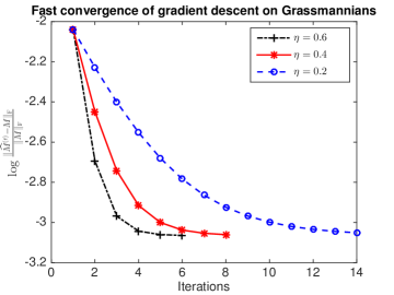
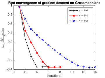
Figure 1: Convergence of Algorithm 1 in relative matrix Frobenius norm and the max-norm, with respect to step size $\eta$ and the number of iterations. The parameters are $d_{1}=d_{2}=d=2000,r=3,\lambda_{i}=d,\sigma_{\xi}=0.6$ and $U,V$ are generated from the SVD of $d\times r$ Rademacher random matrices. The sample size is $n=4r^{2}d\log(d)$ and the noise is Gaussian.

Next, we investigate how the proposed inference tools behave under Gaussian noise and for four different linear forms corresponding to $T_{1}=e_{1}e_{1}^{\mathsf{T}}$, $T_{2}=e_{1}e_{1}^{\mathsf{T}}-e_{1}e_{2}^{\mathsf{T}}$, $T_{3}=e_{1}e_{1}^{\mathsf{T}}-e_{1}e_{2}^{\mathsf{T}}+e_{2}e_{1}^{\mathsf{T}}$ and

$$T_{4}=e_{1}e_{1}^{\mathsf{T}}-e_{1}e_{2}^{\mathsf{T}}+2e_{2}e_{1}^{\mathsf{T}}+3e_{2}e_{2}^{\mathsf{T}}.$$

For each $T$, we drew the density histogram of $(\widehat{m}_{T}-m_{T})/\big{(}\widehat{\sigma}_{\xi}\widehat{s}_{T}\sqrt{d_{1}d_{2}/n}\big{)}$ based on $1000$ independent simulation runs. The density histograms are displayed in Figure 2 where the red curve represents the p.d.f. of standard normal distributions. The sample size was $n=4r^{2}d\log(d)$ for $T_{1},T_{2}$ and $n=5r^{2}d\log(d)$ for $T_{3},T_{4}$. The empirical observation agrees fairly well with our theoretical results.

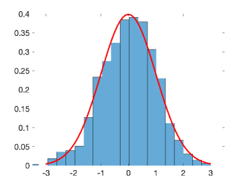
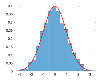
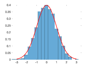
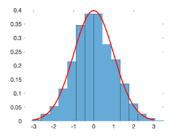
Figure 2: Normal approximation of $\frac{\widehat{m}_{T}-m_{T}}{\widehat{\sigma}_{\xi}\widehat{s}_{T}\sqrt{d_{1}d_{2}/n}}$. The parameters are $d_{1}=d_{2}=d=2000,r=3,\lambda_{i}=d,\sigma_{\xi}=0.6$ and $U,V$ are generated from the SVD of $d\times r$ Rademacher random matrices. The sample size is $n=4r^{2}d\log(d)$ for the top two and $n=5r^{2}d\log(d)$ for bottom two. The noise is Gaussian. Each density histogram is based on 1000 independent simulations and the red curve represents the p.d.f. of standard normal distributions. Top left: $T=e_{1}e_{1}^{\mathsf{T}}$, top right: $T=e_{1}e_{1}^{\mathsf{T}}-e_{1}e_{2}^{\mathsf{T}}$. Bottom left: $T=e_{1}e_{1}^{\mathsf{T}}-e_{1}e_{2}^{\mathsf{T}}+e_{2}e_{1}^{\mathsf{T}}$, bottom right: $T=e_{1}e_{1}^{\mathsf{T}}-e_{1}e_{2}^{\mathsf{T}}+2e_{2}e_{1}^{\mathsf{T}}+3e_{2}e_{2}^{\mathsf{T}}$.

Finally, we examine the performance of the proposed approach under non-Gaussian noise. In particular, we repeated the last set of experiments with noise $(\xi/\sqrt{3}\sigma_{\xi})\in{\rm Unif}([-1,1])$. The density histograms are displayed in Figure 3 where the red curve represents the p.d.f. of standard normal distributions. Again the empirical evidences support the asymptotic normality of the proposed statistic.

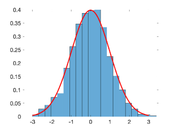
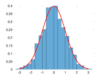
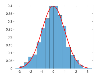
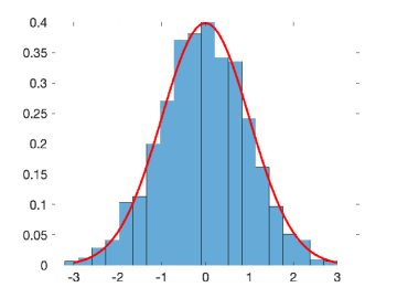
Figure 3: Normal approximation of $\frac{\widehat{m}_{T}-m_{T}}{\widehat{\sigma}_{\xi}\widehat{s}_{T}\sqrt{d_{1}d_{2}/n}}$. The parameters are $d_{1}=d_{2}=d=2000,r=3,\lambda_{i}=d,\sigma_{\xi}=0.6$ and $U,V$ are generated from the SVD of $d\times r$ Rademacher random matrices. The sample size is $n=4r^{2}d\log(d)$ for the top two and $n=5r^{2}d\log(d)$ for the bottom two. The non-Gaussian noise $(\xi/\sqrt{3}\sigma_{\xi})\in{\rm Unif}([-1,1])$. Each density histogram is based on 1000 independent simulations and the red curve represents the p.d.f. of standard normal distributions. Top left: $T=e_{1}e_{1}^{\mathsf{T}}$, top right: $T=e_{1}e_{1}^{\mathsf{T}}-e_{1}e_{2}^{\mathsf{T}}$. Bottom left: $T=e_{1}e_{1}^{\mathsf{T}}-e_{1}e_{2}^{\mathsf{T}}+e_{2}e_{1}^{\mathsf{T}}$, bottom right: $T=e_{1}e_{1}^{\mathsf{T}}-e_{1}e_{2}^{\mathsf{T}}+2e_{2}e_{1}^{\mathsf{T}}+3e_{2}e_{2}^{\mathsf{T}}$.

6.2 Real-world data examples

We now turn our attention to two real-world data examples – the Jester and MovieLens datasets. The Jester dataset contains ratings of $100$ jokes from $\sim 70K$ users (goldberg2001eigentaste). The dataset consists of 3 subsets of data with different characteristics as summarized in Table 1. For each subset, the numbers of ratings of all users are equal. MovieLens was a recommender system created by GroupLens that recommends movies for its users. We use three datasets released by MovieLens (harper2016movielens) whose details are summarized in Table 1. In these three datasets, each user rates at least $20$ movies.

Table 1: Summary of Datasets

Dataset #users #jokes #ratings per user rating values Jester-1 24983 100 $29$ [-10, 10] Jester-2 23500 100 $34$ [-10, 10] Jester-3 24938 100 $14$ [-10, 10] Dataset #users #movies total #ratings rating values ml-100k 943 1682 $\sim 10^{5}$ {1,2,3,4,5} ml-1m 6040 3952 $\sim 10^{6}$ {1,2,3,4,5} ml-10m 71567 10681 $\sim 10^{7}$ $\{0.5,1.0,\cdots,4.5,5.0\}$

For illustration, we consider the task of recommending jokes or movies to a particular users. Because of the lack of ground truth, we resort to resampling. For the Jester dataset, we randomly sample $\sim 2000$ users, and for each user $2$ ratings that at least $\zeta\in\{0,2,6,10,14\}$ apart. We removed these ratings from the training and used the proposed procedure to infer, for each user ($i$), between these two jokes ($j_{1}$ or $j_{2}$) with ratings which one should be recommended. This amounts to the following one-sided tests:

$$H_{0}:M(i,j_{1})\leq M(i,j_{2})\quad{\rm v.s.}\quad H_{1}:M(i,j_{1})>M(i,j_{2}).$$

We ran the proposed procedure on the training data and evaluate the test statistic $\hat{z}$ for each user from the testing set. In particular, we fixed the rank $r=2$ corresponding to the smallest estimate $\hat{\sigma}_{\xi}$. Note that we do not know the true value of $M(i,j)$ and only observe $Y(i,j)=M(i,j)+\xi(i,j)$. We therefore use ${\mathbb{I}}(Y(i,j_{1})>Y(i,j_{2}))$ as a proxy to differentiate between $H_{0}$ and $H_{1}$. Assuming that the $\xi$ has a distribution symmetric about 0, then ${\mathbb{I}}(Y(i,j_{1})>Y(i,j_{2}))$ is more likely to take value $0$ under $H_{0}$, and $1$ under $H_{1}$. We shall evaluate the performance of our procedure based on its discriminant power in predicting ${\mathbb{I}}(Y(i,j_{1})>Y(i,j_{2}))$. In particular, we record the ROC curve of $\hat{z}$ for all users from the testing set. The results, averaged over $10$ simulation runs for each value of $\zeta$, are reported in Figure 4. Clearly, we can observe an increase in predictive power as $\zeta$ increases suggesting $\hat{z}$ as a reasonable statistic for testing $H_{0}$ against $H_{1}$.

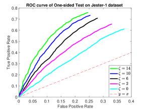
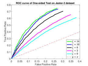
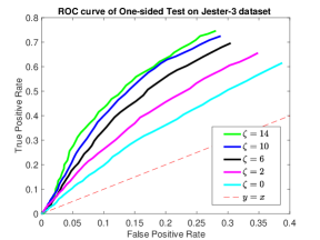
Figure 4: ROC curves for one-sided tests $H_{0}:M(i,j_{1})\leq M(i,j_{2})\ {\rm v.s.}\ H_{1}:M(i,j_{1})>M(i,j_{2})$ on Jester datasets. The testing data are sampled such that $|Y(i,j_{1})-Y(i,j_{2})|\geq\zeta$. The estimated noise level $\hat{\sigma}_{\xi}=4.5160$ on Jester-1, $\hat{\sigma}_{\xi}=4.4843$ on Jester-2, and $\hat{\sigma}_{\xi}=5.1152$ on Jester-3. The rightmost point of each ROC curve corresponds to the significance level $\theta=0.5$ so that $z_{\theta}=0$.

We ran a similar experiment on the MovieLens datasets. In each simulation run, we randomly sampled $\sim 800$ users and $2$ ratings each as the test data. These ratings are sampled such that $|Y(i,j_{1})-Y(i,j_{2})|\geq\zeta$ for $\zeta=0,1,2,3,4$. The false positive rates and true positive rates of our proposed procedure were again recorded. The ROC curves, averaged again over $10$ runs for each value of $\zeta$, are shown in Figure 5. This again indicates a reasonable performance of the proposed testing procedure. Empirically, we observe a better de-biasing approach on these datasets which is $\widehat{M}_{1}^{\scriptscriptstyle\sf unbs}=\widehat{M}_{1}^{\scriptscriptstyle\sf init}+\sum_{i\in\mathfrak{D}_{2}}(Y_{i}-\langle\widehat{M}_{1}^{\scriptscriptstyle\sf init},X_{i}\rangle)X_{i}$. The rationale is to partially replace $\widehat{M}_{1}^{\scriptscriptstyle\sf init}$’s entries with the observed training ratings. This improvement might be due to the severe heterogeneity in the numbers of observed ratings from distinct users, or due to the unknown noise distributions.

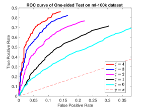
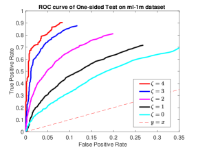
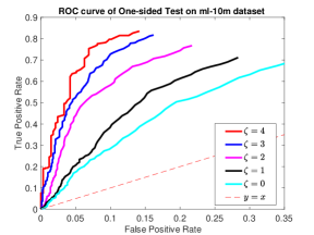
Figure 5: ROC curves for one-sided tests $H_{0}:M(i,j_{1})\leq M(i,j_{2})\ {\rm v.s.}\ H_{1}:M(i,j_{1})>M(i,j_{2})$ on MovieLens datasets. The testing data are sampled such that $|Y(i,j_{1})-Y(i,j_{2})|\geq\zeta$. The estimated noise level $\hat{\sigma}_{\xi}=0.9973$ on ml-100k, $\hat{\sigma}_{\xi}=0.8936$ on ml-1m, and $\hat{\sigma}_{\xi}=0.9151$ on ml-10m. The rightmost point of each ROC curve corresponds to the significance level $\theta=0.5$ so that $z_{\theta}=0$.

7 Proofs

Throughout the proof, we write $\gamma_{n}$ in short for $\gamma_{n,d_{1},d_{2}}$.

7.1 De-localized perturbation of singular vectors

Essential to our proofs is the precise characterization of the empirical singular spaces. To this end, we shall first develop bounds for the estimation error of $\widehat{U}_{1},\widehat{U}_{2},\widehat{V}_{1}$ and $\widehat{V}_{2}$. Recall that the matrix $(2,{\rm max})$-norm is defined as $\|A\|_{\scriptscriptstyle\sf 2,max}=\max_{j\in[d_{1}]}\|e_{j}^{\mathsf{T}}A\|$. This can be naturally extended to a distance on Grassmannians

$$d_{\scriptscriptstyle\sf 2,max}(U_{1},U_{2}):=\|U_{1}U_{1}^{\mathsf{T}}-U_{2}U_{2}^{\mathsf{T}}\|_{\scriptscriptstyle\sf 2,max},$$

for $U_{1},U_{2}\in\mathbb{O}^{d\times r}$. The main goal of this subsection is to establish the following result:

Theorem 4.

Under Assumptions 1-3, there exists an absolute constant $C>0$ such that if $n\geq C\mu_{\scriptscriptstyle\sf max}^{2}rd_{1}\log d_{1}$, then with probability at least $1-5d_{1}^{-2}\log d_{1}$,

$$d_{\scriptscriptstyle\sf 2,max}(\widehat{U}_{i},U)\leq C_{2}\mu_{\scriptscriptstyle\sf max}\frac{(1+\gamma_{n})\sigma_{\xi}}{\lambda_{r}}\cdot\sqrt{\frac{rd_{2}d_{1}\log d_{1}}{n}}$$

and

$$d_{\scriptscriptstyle\sf 2,max}(\widehat{V}_{i},V)\leq C_{2}\mu_{\scriptscriptstyle\sf max}\frac{(1+\gamma_{n})\sigma_{\xi}}{\lambda_{r}}\cdot\sqrt{\frac{rd_{1}^{2}\log d_{1}}{n}}$$

for $i=1,2$ and some absolute constant $C_{2}>0$.

Immediately following Theorem 4 and Assumption 3, we know that

$$\big{\|}e_{j}^{\mathsf{T}}\widehat{U}_{1}\big{\|}=\big{\|}e_{j}^{\mathsf{T}} (\widehat{U}_{1}\widehat{U}_{1}^{\mathsf{T}}-UU^{\mathsf{T}})\widehat{U}_{1}\big{\|}+\big{\|}e_{j}^{\mathsf{T}}UU^{\mathsf{T}}\widehat{U}_{1}\big{\|}$$

$$\leq C_{2}\frac{\sigma_{\xi}}{\lambda_{r}}\sqrt{\frac{d_{1}^{2}d_{2}\log d_{1}}{n}}\cdot\mu_{\scriptscriptstyle\sf max}\sqrt{\frac{r}{d_{1}}}+\|e_{j}^{\mathsf{T}}U\|\leq 2\mu_{\scriptscriptstyle\sf max}\sqrt{\frac{r}{d_{1}}}.$$

Then, we conclude that

$$\|\widehat{U}_{i}\|_{\scriptscriptstyle\sf 2,max}\leq 2\mu_{\scriptscriptstyle\sf max}\sqrt{\frac{r}{d_{1}}}\quad{\rm and}\quad\|\widehat{V}_{i}\|_{\scriptscriptstyle\sf 2,max}\leq 2\mu_{\scriptscriptstyle\sf max}\sqrt{\frac{r}{d_{2}}},\quad\forall i=1,2,$$

an observation that we shall repeatedly use in the following subsections.

7.1.1 Preliminary bounds

Denote $\widehat{\Delta}_{1}=M-\widehat{M}_{1}^{\scriptscriptstyle\sf init}$ and $\widehat{\Delta}_{2}=M-\widehat{M}_{2}^{\scriptscriptstyle\sf init}$. We then write

$$\widehat{M}_{1}^{\scriptscriptstyle\sf unbs}=M+\underbrace{\frac{d_{1}d_{2}}{n_{0}}\sum_{i=n_{0}+1}^{n}\xi_{i}X_{i}}_{\widehat{Z}_{1}^{(1)}}+\underbrace{\Big{(}\frac{d_{1}d_{2}}{n_{0}}\sum_{i=n_{0}+1}^{n}\langle\widehat{\Delta}_{1},X_{i}\rangle X_{i}-\widehat{\Delta}_{1}\Big{)}}_{\widehat{Z}_{2}^{(1)}}$$ (7.1)

and

$$\widehat{M}_{2}^{\scriptscriptstyle\sf unbs}=M+\underbrace{\frac{d_{1}d_{2}}{n_{0}}\sum_{i=1}^{n_{0}}\xi_{i}X_{i}}_{\widehat{Z}_{1}^{(2)}}+\underbrace{\Big{(}\frac{d_{1}d_{2}}{n_{0}}\sum_{i=1}^{n_{0}}\langle\widehat{\Delta}_{2},X_{i}\rangle X_{i}-\widehat{\Delta}_{2}\Big{)}}_{\widehat{Z}_{2}^{(2)}},$$ (7.2)

where $\widehat{\Delta}_{1}$ is independent with $\{(X_{i},\xi_{i})\}_{i=n_{0}+1}^{n}$, and $\widehat{\Delta}_{2}$ is independent with $\{(X_{i},\xi_{i})\}_{i=1}^{n_{0}}$. Denote $\widehat{Z}^{(i)}=\widehat{Z}_{1}^{(i)}+\widehat{Z}_{2}^{(i)}$ and then $\widehat{M}_{i}^{\scriptscriptstyle\sf unbs}=M+\widehat{Z}^{(i)}$ for $i=1,2$. Clearly, $\mathbb{E}\widehat{Z}^{(i)}=\mathbb{E}\widehat{Z}_{1}^{(i)}+\mathbb{E}\widehat{Z}_{2}^{(i)}=0$.

Observe that eq. (7.1, 7.2) admit explicit representation formulas for $\widehat{M}_{1}^{\scriptscriptstyle\sf unbs},\widehat{M}_{2}^{\scriptscriptstyle\sf unbs}$. Meanwhile, because $\|\widehat{\Delta}_{1}\|_{\scriptscriptstyle\sf max},\|\widehat{\Delta}_{2}\|_{\scriptscriptstyle\sf max}=o_{P}(\sigma_{\xi})$, the strength of $\widehat{Z}^{(1)}_{2}$ and $\widehat{Z}^{(2)}_{2}$ are dominated by that of $\widehat{Z}^{(1)}_{1}$ and $\widehat{Z}^{(2)}_{1}$, respectively. Observe that the perturbation by $\widehat{Z}^{(1)}_{1}$ is analogous (or close) to a random perturbation with i.id. entry-wise noise. Put it differently, the debiasing treatment by (7.1,7.2) is essentially to re-randomize $\widehat{M}_{1}^{\scriptscriptstyle\sf init}$ and $\widehat{M}_{2}^{\scriptscriptstyle\sf init}$. It plays the key role in characterizing the distributions of $\widehat{U}_{1},\widehat{U}_{2}$ and $\widehat{V}_{1},\widehat{V}_{2}$.

We begin with several preliminary properties of $\{\widehat{U}_{i}\}_{i=1}^{2}$ and $\{\widehat{V}_{i}\}_{i=1}^{2}$. Recall that $\widehat{U}_{1}$ and $\widehat{V}_{1}$ are top-$r$ left and right singular vectors of $\widehat{M}_{1}^{\scriptscriptstyle\sf unbs}=M+\widehat{Z}_{1}^{(1)}+\widehat{Z}_{2}^{(1)}$. The following bounds for $\widehat{Z}^{(i)}_{j}$s are useful for our derivation.

Lemma 1.

There exist absolute constants $C_{1},C_{2}>0$ such that if $n\geq C_{1}d_{1}\log d_{1}$, with probability at least $1-2d_{1}^{-2}$, the following bounds hold for $i=1,2$

$$\big{\|}\widehat{Z}_{1}^{(i)}\big{\|}\leq C_{2}\sigma_{\xi}\sqrt{\frac{d_{1}^{2}d_{2}\log d_{1}}{n}}\quad{\rm and}\quad\big{\|}\widehat{Z}_{2}^{(i)}\big{\|}\leq C_{2}\|\widehat{\Delta}_{i}\|_{\scriptscriptstyle\sf max}\sqrt{\frac{d_{1}^{2}d_{2}\log d_{1}}{n}},$$

where the probability of the second inequality is conditioned on $\widehat{\Delta}_{i}$.

We shall defer the proof of Lemma 1 to the Appendix. These bounds can be readily used to derive bounds for the empirical singular vectors under Frobenius-norm distance and operator-norm distance. Recall that for $U_{1},U_{2}\in\mathbb{O}^{d\times r}$, the Frobenius-norm distance and operator-norm distance are defined by

$$d_{\scriptscriptstyle\sf F}(U_{1},U_{2})=\|U_{1}U_{1}^{\mathsf{T}}-U_{2}U_{2}^{\mathsf{T}}\|_{\scriptscriptstyle\sf F}\quad{\rm and}\quad d_{\scriptscriptstyle\sf O}(U_{1},U_{2})=\|U_{1}U_{1}^{\mathsf{T}}-U_{2}U_{2}^{\mathsf{T}}\|.$$

It is well known that

$$\min_{O\in\mathbb{O}^{r\times r}}\|U_{1}-U_{2}O\|_{\scriptscriptstyle\sf F}\leq\sqrt{2}d_{\scriptscriptstyle\sf F}(U_{1},U_{2})\leq\sqrt{2}\cdot\min_{O\in\mathbb{O}^{r\times r}}\|U_{1}-U_{2}O\|_{\scriptscriptstyle\sf F}$$

and

$$\min_{O\in\mathbb{O}^{r\times r}}\|U_{1}-U_{2}O\|\leq\sqrt{2}d_{\scriptscriptstyle\sf O}(U_{1},U_{2})\leq\sqrt{2}\cdot\min_{O\in\mathbb{O}^{r\times r}}\|U_{1}-U_{2}O\|.$$

See, e.g., Edelman et al. (1998).

Lemma 2.

Under Assumptions 1-3, there exists an absolute constant $C>0$ such that if $n\geq Cd_{1}\log d_{1}$, then with probability at least $1-2d_{1}^{-2}$,

$$\max\{d_{\scriptscriptstyle\sf F}(\widehat{U}_{i},U),d_{\scriptscriptstyle\sf F}(\widehat{V}_{i},V)\}\leq C_{2}\frac{(1+\gamma_{n})\sigma_{\xi}}{\lambda_{r}}\cdot\sqrt{\frac{rd_{1}^{2}d_{2}\log{d_{1}}}{n}}\quad\textrm{ for }i=1,2,$$

and

$$\max\{d_{\scriptscriptstyle\sf O}(\widehat{U}_{i},U),d_{\scriptscriptstyle\sf O}(\widehat{V}_{i},V)\}\leq C_{2}\frac{(1+\gamma_{n})\sigma_{\xi}}{\lambda_{r}}\cdot\sqrt{\frac{d_{1}^{2}d_{2}\log d_{1}}{n}}\quad\textrm{ for }i=1,2,$$

where $C_{2}>0$ is an absolute constant and $\gamma_{n}$ is defined by Assumption 1.

7.2 Proof of Theorem 1

We are now in position to prove Theorem 1. Recall that

$$\widehat{m}_{T}-m_{T}= \frac{1}{2}\big{<}\widehat{U}_{1}\widehat{U}_{1}^{\mathsf{T}}\widehat{Z}^{(1)}\widehat{V}_{1}\widehat{V}_{1}^{\mathsf{T}},T\big{>}+\frac{1}{2}\big{<}\widehat{U}_{2}\widehat{U}_{2}^{\mathsf{T}}\widehat{Z}^{(2)}\widehat{V}_{2}\widehat{V}_{2}^{\mathsf{T}},T\big{>}$$

$$+\frac{1}{2}\big{<}\widehat{U}_{1}\widehat{U}_{1}^{\mathsf{T}}M\widehat{V}_{1}\widehat{V}_{1}^{\mathsf{T}}-M,T\big{>}+\frac{1}{2}\big{<}\widehat{U}_{2}\widehat{U}_{2}^{\mathsf{T}}M\widehat{V}_{2}\widehat{V}_{2}^{\mathsf{T}}-M,T\big{>}.$$

Our strategy is to show that $\big{\{}\big{|}\big{<}\widehat{U}_{i}\widehat{U}_{i}^{\mathsf{T}}\widehat{Z}^{(i)}\widehat{V}_{i}\widehat{V}_{i}^{\mathsf{T}},T\big{>}\big{|}\big{\}}_{i=1}^{2}$ are negligible. Then, we prove the normal approximation of $\big{\{}\big{<}\widehat{U}_{i}\widehat{U}_{i}^{\mathsf{T}}M\widehat{V}_{i}\widehat{V}_{i}^{\mathsf{T}}-M,T\big{>}\big{\}}_{i=1}^{2}$. We begin with the upper bounds of $\big{\{}\big{|}\big{<}\widehat{U}_{i}\widehat{U}_{i}^{\mathsf{T}}\widehat{Z}^{(i)}\widehat{V}_{i}\widehat{V}_{i}^{\mathsf{T}},T\big{>}\big{|}\big{\}}_{i=1}^{2}$.

Lemma 3.

Under Assumptions 1-3, and conditioned on the event in Theorem 4, there exist absolute constants $C_{1},C_{2}>0$ such that with probability at least $1-2d_{1}^{-2}$,

$$\big{|}\big{<}\widehat{U}_{i}\widehat{U}_{i}^{\mathsf{T}}\widehat{Z}^{(i)}\widehat{V}_{i}\widehat{V}_{i}^{\mathsf{T}},T\big{>}\big{|}\leq C_{1} \|T\|_{\ell_{1}}\mu_{\scriptscriptstyle\sf max}^{2}\sigma_{\xi}\sqrt{\frac{r\log d_{1}}{n}}$$

$$+C_{2}\|T\|_{\ell_{1}}\mu_{\scriptscriptstyle\sf max}^{2}\frac{\sigma_{\xi}}{\lambda_{r}}\sqrt{\frac{rd_{1}^{2}d_{2}\log d_{1}}{n}}\cdot\sigma_{\xi}\sqrt{\frac{rd_{1}\log d_{1}}{n}}.$$

We now prove the normal approximation of

$$\frac{1}{2}\big{<}\widehat{U}_{1}\widehat{U}_{1}^{\mathsf{T}}M\widehat{V}_{1}\widehat{V}_{1}^{\mathsf{T}}-M,T\big{>}+\frac{1}{2}\big{<}\widehat{U}_{2}\widehat{U}_{2}^{\mathsf{T}}M\widehat{V}_{2}\widehat{V}_{2}^{\mathsf{T}}-M,T\big{>}.$$

Let $\Theta$ and $A$ be defined as in the proof of Theorem 4. Moreover, we define

$$\widehat{\Theta}_{1}=\left(\begin{array}[]{cc}\widehat{U}_{1}&0\\ 0&\widehat{V}_{1}\end{array}\right)\quad{\rm and}\quad\widehat{\Theta}_{2}=\left(\begin{array}[]{cc}\widehat{U}_{2}&0\\ 0&\widehat{V}_{2}\end{array}\right).$$

Then, we write

$$\widehat{\Theta}_{1}\widehat{\Theta}_{1}^{\mathsf{T}}A\widehat{\Theta}_{1}\widehat{\Theta}_{1}^{\mathsf{T}}-\Theta\Theta^{\mathsf{T}}A\Theta\Theta^{\mathsf{T}}=\left(\begin{array}[]{cc}0&\widehat{U}_{1}\widehat{U}_{1}^{\mathsf{T}}M\widehat{V}_{1}\widehat{V}_{1}^{\mathsf{T}}-M\\ (\widehat{U}_{1}\widehat{U}_{1}^{\mathsf{T}}M\widehat{V}_{1}\widehat{V}_{1}^{\mathsf{T}}-M)^{\mathsf{T}}&0\end{array}\right)$$

and

$$\widehat{\Theta}_{2}\widehat{\Theta}_{2}^{\mathsf{T}}A\widehat{\Theta}_{2}\widehat{\Theta}_{2}^{\mathsf{T}}-\Theta\Theta^{\mathsf{T}}A\Theta\Theta^{\mathsf{T}}=\left(\begin{array}[]{cc}0&\widehat{U}_{2}\widehat{U}_{2}^{\mathsf{T}}M\widehat{V}_{2}\widehat{V}_{2}^{\mathsf{T}}-M\\ (\widehat{U}_{2}\widehat{U}_{2}^{\mathsf{T}}M\widehat{V}_{2}\widehat{V}_{2}^{\mathsf{T}}-M)^{\mathsf{T}}&0\end{array}\right).$$

Denote

$$\widetilde{T}=\left(\begin{array}[]{cc}0&T\\ 0&0\end{array}\right)\quad{\rm and}\quad\widehat{E}^{(i)}=\left(\begin{array}[]{cc}0&\widehat{Z}^{(i)}\\ \widehat{Z}^{(i)\mathsf{T}}&0\end{array}\right)\quad\forall i=1,2.$$

Therefore, we have

$$\frac{1}{2}\big{<}\widehat{U}_{1}\widehat{U}_{1}^{\mathsf{T}}M\widehat{V}_{1}\widehat{V}_{1}^{\mathsf{T}} -M,T\big{>}+\frac{1}{2}\big{<}\widehat{U}_{2}\widehat{U}_{2}^{\mathsf{T}}M\widehat{V}_{2}\widehat{V}_{2}^{\mathsf{T}}-M,T\big{>}$$

$$= \frac{1}{2}\big{<}\widehat{\Theta}_{1}\widehat{\Theta}_{1}^{\mathsf{T}}A\widehat{\Theta}_{1}\widehat{\Theta}_{1}^{\mathsf{T}}-\Theta\Theta^{\mathsf{T}}A\Theta\Theta^{\mathsf{T}},\widetilde{T}\big{>}+\frac{1}{2}\big{<}\widehat{\Theta}_{2}\widehat{\Theta}_{2}^{\mathsf{T}}A\widehat{\Theta}_{2}\widehat{\Theta}_{2}^{\mathsf{T}}-\Theta\Theta^{\mathsf{T}}A\Theta\Theta^{\mathsf{T}},\widetilde{T}\big{>}.$$

By (7.11), we write

$$\widehat{\Theta}_{i}\widehat{\Theta}_{i}^{\mathsf{T}}-\Theta\Theta^{\mathsf{T}}=\sum_{k=1}^{\infty}{\cal S}_{A,k}(\widehat{E}^{(i)})\quad\forall i=1,2,$$

and as a result, for $i=1,2$,

$$\widehat{\Theta}_{i}\widehat{\Theta}_{i}^{\mathsf{T}}A \widehat{\Theta}\widehat{\Theta}^{\mathsf{T}}-\Theta\Theta^{\mathsf{T}}A\Theta\Theta^{\mathsf{T}}$$

$$= \big{(}{\cal S}_{A,1}(\widehat{E}^{(i)})A\Theta\Theta^{\mathsf{T}}+\Theta\Theta^{\mathsf{T}}A{\cal S}_{A,1}(\widehat{E}^{(i)})\big{)}+\sum_{k=2}^{\infty}\big{(}{\cal S}_{A,k}(\widehat{E}^{(i)})A\Theta\Theta^{\mathsf{T}}+\Theta\Theta^{\mathsf{T}}A{\cal S}_{A,k}(\widehat{E}^{(i)})\big{)}$$

$$\hskip 56.9055pt+(\widehat{\Theta}_{i}\widehat{\Theta}_{i}^{\mathsf{T}}-\Theta\Theta^{\mathsf{T}})A(\widehat{\Theta}_{i}\widehat{\Theta}_{i}^{\mathsf{T}}-\Theta\Theta^{\mathsf{T}}).$$

Then, we write

$$\frac{1}{2}\big{<}\widehat{U}_{1}\widehat{U}_{1}^{\mathsf{T}}M\widehat{V}_{1}\widehat{V}_{1}^{\mathsf{T}} -M,T\big{>}+\frac{1}{2}\big{<}\widehat{U}_{2}\widehat{U}_{2}^{\mathsf{T}}M\widehat{V}_{2}\widehat{V}_{2}^{\mathsf{T}}-M,T\big{>}$$

$$= \frac{1}{2}\sum_{i=1}^{2}\big{<}\big{(}{\cal S}_{A,1}(\widehat{E}^{(i)})A\Theta\Theta^{\mathsf{T}}+\Theta\Theta^{\mathsf{T}}A{\cal S}_{A,1}(\widehat{E}^{(i)})\big{)},\widetilde{T}\big{>}$$

$$+ \frac{1}{2}\sum_{i=1}^{2}\sum_{k=2}^{\infty}\big{<}\big{(}{\cal S}_{A,k}(\widehat{E}^{(i)})A\Theta\Theta^{\mathsf{T}}+\Theta\Theta^{\mathsf{T}}A{\cal S}_{A,k}(\widehat{E}^{(i)})\big{)},\widetilde{T}\big{>}$$

$$+ \frac{1}{2}\sum_{i=1}^{2}\big{<}(\widehat{\Theta}_{i}\widehat{\Theta}_{i}^{\mathsf{T}}-\Theta\Theta^{\mathsf{T}})A(\widehat{\Theta}_{i}\widehat{\Theta}_{i}^{\mathsf{T}}-\Theta\Theta^{\mathsf{T}}),\widetilde{T}\big{>}.$$

By the definition of ${\cal S}_{A,1}(\widehat{E}^{(i)})$, we write

$$\frac{1}{2}\sum_{i=1}^{2}\big{<}{\cal S}_{A,1} (\widehat{E}^{(i)})A\Theta\Theta^{\mathsf{T}}+\Theta\Theta^{\mathsf{T}}A{\cal S}_{A,1}(\widehat{E}^{(i)}),\widetilde{T}\big{>}$$

$$= \langle U_{\perp}U_{\perp}^{\mathsf{T}}(\widehat{Z}^{(1)}/2+\widehat{Z}^{(2)}/2)VV^{\mathsf{T}},T\rangle+\langle UU^{\mathsf{T}}(\widehat{Z}^{(1)}/2+\widehat{Z}^{(2)}/2)V_{\perp}V_{\perp}^{\mathsf{T}},T\rangle.$$

We begin with the normal approximation of $\frac{1}{2}\sum_{i=1}^{2}\big{<}{\cal S}_{A,1}(\widehat{E}^{(i)})A\Theta\Theta^{\mathsf{T}}+\Theta\Theta^{\mathsf{T}}A{\cal S}_{A,1}(\widehat{E}^{(i)}),\widetilde{T}\big{>}$.

Lemma 4.

Under Assumptions 1-3 and suppose that $n\geq C_{1}\mu_{\scriptscriptstyle\sf max}^{2}rd_{1}\log d_{1}$, we have

$$\sup_{x\in\mathbb{R}}\bigg{|}\mathbb{P}\bigg{(} \frac{\frac{1}{2}\sum_{i=1}^{2}\big{<}{\cal S}_{A,1}(\widehat{E}^{(i)})A\Theta\Theta^{\mathsf{T}}+\Theta\Theta^{\mathsf{T}}A{\cal S}_{A,1}(\widehat{E}^{(i)}),\widetilde{T}\big{>}}{\sigma_{\xi}(\|V^{\mathsf{T}}T^{\mathsf{T}}\|_{\scriptscriptstyle\sf F}^{2}+\|U^{\mathsf{T}}T\|_{\scriptscriptstyle\sf F}^{2})^{1/2}\cdot\sqrt{d_{1}d_{2}/n}}\leq x\bigg{)}-\Phi(x)\bigg{|}$$

$$\hskip 56.9055pt\leq C_{2}\frac{\mu_{\scriptscriptstyle\sf max}^{4}\|T\|_{\ell_{1}}^{2}}{\alpha_{T}^{2}\|T\|_{\scriptscriptstyle\sf F}^{2}}\cdot\frac{r\sqrt{\log d_{1}}}{d_{2}}+\frac{3}{d_{1}^{2}}+C_{3}\gamma_{n}\sqrt{\log d_{1}}+C_{4}\mu_{\scriptscriptstyle\sf max}\sqrt{\frac{rd_{1}}{n}}.$$

where $C_{1},C_{2},C_{3},C_{4}>0$ are absolute constants and $\gamma_{n}$ is defined by Assumption 1.

Lemma 5 and Lemma 6 characterize sharp bounds for the remainder terms.

Lemma 5.

Under Assumptions 1-3, under the event of Theorem 4,

$$\big{|}\sum_{i=1}^{2}\sum_{k=2}^{\infty}\big{<}\big{(}{\cal S}_{A,k}(\widehat{E}^{(i)}) A\Theta\Theta^{\mathsf{T}}+\Theta\Theta^{\mathsf{T}}A{\cal S}_{A,k}(\widehat{E}^{(i)})\big{)},\widetilde{T}\big{>}\big{|}$$

$$\leq C_{2}\|T\|_{\ell_{1}}\mu_{\scriptscriptstyle\sf max}^{2}\sigma_{\xi}\sqrt{\frac{rd_{1}\log d_{1}}{n}}\cdot\Big{(}\frac{\sigma_{\xi}}{\lambda_{r}}\cdot\sqrt{\frac{rd_{1}^{2}d_{2}\log d_{1}}{n}}\Big{)},$$

where $C_{2}>0$ is some absolute constant.

Lemma 6.

Under Assumptions 1-3, on the event of Theorem 4,

$$\sum_{i=1}^{2}\big{|}\big{<}(\widehat{\Theta}_{i}\widehat{\Theta}_{i}^{\mathsf{T}}-\Theta \Theta^{\mathsf{T}})A(\widehat{\Theta}_{i}\widehat{\Theta}_{i}^{\mathsf{T}}-\Theta\Theta^{\mathsf{T}}),\widetilde{T}\big{>}\big{|}$$

$$\leq C_{2}\kappa_{0}\mu_{\scriptscriptstyle\sf max}^{2}\|T\|_{\ell_{1}}\sigma_{\xi}\sqrt{\frac{rd_{1}\log d_{1}}{n}}\cdot\frac{\sigma_{\xi}}{\lambda_{r}}\sqrt{\frac{rd_{1}^{2}d_{2}\log d_{1}}{n}}$$

for some absolute constant $C_{2}>0$ and $\kappa(M)\leq\kappa_{0}$ denotes $M$’s condition number.

We write

$$\frac{\widehat{m}_{T}-m_{T}}{\sigma_{\xi}(\|V^{\mathsf{T}}T^{\mathsf{T}}\|_{\scriptscriptstyle\sf F}^{2}+\|U^{\mathsf{T}}T\|_{\scriptscriptstyle\sf F}^{2})^{1/2}\cdot\sqrt{d_{1}d_{2}/n}}$$

$$\hskip 56.9055pt=\frac{\sum_{i=1}^{2}\langle\widehat{U}_{i}\widehat{U}_{i}^{\mathsf{T}}\widehat{Z}^{(i)}\widehat{V}_{i}\widehat{V}_{i}^{\mathsf{T}},T\rangle/2}{\sigma_{\xi}(\|V^{\mathsf{T}}T^{\mathsf{T}}\|_{\scriptscriptstyle\sf F}^{2}+\|U^{\mathsf{T}}T\|_{\scriptscriptstyle\sf F}^{2})^{1/2}\cdot\sqrt{d_{1}d_{2}/n}}$$

$$\hskip 56.9055pt+\frac{\sum_{i=1}^{2}\big{<}{\cal S}_{A,1}(\widehat{E}^{(i)})A\Theta\Theta^{\mathsf{T}}+\Theta\Theta^{\mathsf{T}}A{\cal S}_{A,1}(\widehat{E}^{(i)}),\widetilde{T}\big{>}/2}{\sigma_{\xi}(\|V^{\mathsf{T}}T^{\mathsf{T}}\|_{\scriptscriptstyle\sf F}^{2}+\|U^{\mathsf{T}}T\|_{\scriptscriptstyle\sf F}^{2})^{1/2}\cdot\sqrt{d_{1}d_{2}/n}}$$

$$\hskip 56.9055pt+\frac{\sum_{i=1}^{2}\sum_{k=2}^{\infty}\big{<}\big{(}{\cal S}_{A,k}(\widehat{E}^{(i)})A\Theta\Theta^{\mathsf{T}}+\Theta\Theta^{\mathsf{T}}A{\cal S}_{A,k}(\widehat{E}^{(i)})\big{)},\widetilde{T}\big{>}/2}{\sigma_{\xi}(\|V^{\mathsf{T}}T^{\mathsf{T}}\|_{\scriptscriptstyle\sf F}^{2}+\|U^{\mathsf{T}}T\|_{\scriptscriptstyle\sf F}^{2})^{1/2}\cdot\sqrt{d_{1}d_{2}/n}}$$

$$\hskip 56.9055pt+\frac{\sum_{i=1}^{2}\big{<}(\widehat{\Theta}_{i}\widehat{\Theta}_{i}^{\mathsf{T}}-\Theta\Theta^{\mathsf{T}})A(\widehat{\Theta}_{i}\widehat{\Theta}_{i}^{\mathsf{T}}-\Theta\Theta^{\mathsf{T}}),\widetilde{T}\big{>}/2}{\sigma_{\xi}(\|V^{\mathsf{T}}T^{\mathsf{T}}\|_{\scriptscriptstyle\sf F}^{2}+\|U^{\mathsf{T}}T\|_{\scriptscriptstyle\sf F}^{2})^{1/2}\cdot\sqrt{d_{1}d_{2}/n}}.$$

Under Assumption 4, it holds that $\|V^{\mathsf{T}}T^{\mathsf{T}}\|_{\scriptscriptstyle\sf F}^{2}+\|U^{\mathsf{T}}T\|_{\scriptscriptstyle\sf F}^{2}\geq\alpha_{T}^{2}\|T\|_{\scriptscriptstyle\sf F}^{2}r/d_{1}$. As a result,

$$\sigma_{\xi}(\|V^{\mathsf{T}}T^{\mathsf{T}}\|_{\scriptscriptstyle\sf F}^{2}+\|U^{\mathsf{T}}T\|_{\scriptscriptstyle\sf F}^{2})^{1/2}\cdot\sqrt{d_{1}d_{2}/n}\geq\alpha_{T}\|T\|_{\scriptscriptstyle\sf F}\sigma_{\xi}\sqrt{\frac{rd_{2}}{n}}.$$

Together with Lemma 3,5 and Lemma 6, we get, with probability at least $1-6d_{1}^{-2}\log d_{1}$, that

$$\frac{\big{|}(\widehat{m}_{T}-m_{T})-\sum_{i=1}^{2}\big{<}{\cal S}_{A,1}(\widehat{E}^{(i)})A\Theta\Theta^{\mathsf{T}}+\Theta\Theta^{\mathsf{T}}A{\cal S}_{A,1}(\widehat{E}^{(i)}),\widetilde{T}\big{>}/2\big{|}}{\sigma_{\xi}(\|V^{\mathsf{T}}T^{\mathsf{T}}\|_{\scriptscriptstyle\sf F}^{2}+\|U^{\mathsf{T}}T\|_{\scriptscriptstyle\sf F}^{2})^{1/2}\cdot\sqrt{d_{1}d_{2}/n}}$$

$$\hskip 28.45274pt\leq C_{1}\frac{\mu_{\scriptscriptstyle\sf max}^{2}\|T\|_{\ell_{1}}}{\alpha_{T}\|T\|_{\scriptscriptstyle\sf F}}\cdot\sqrt{\frac{\log d_{1}}{d_{2}}}+C_{2}\kappa_{0}\frac{\mu_{\scriptscriptstyle\sf max}^{2}\|T\|_{\ell_{1}}}{\alpha_{T}\|T\|_{\scriptscriptstyle\sf F}}\cdot\frac{\sigma_{\xi}}{\lambda_{r}}\sqrt{\frac{\alpha_{d}rd_{1}^{2}d_{2}\log^{2}d_{1}}{n}}$$

for some absolute constants $C_{1},C_{2}>0$. By the normal approximation of $\sum_{i=1}^{2}\big{<}{\cal S}_{A,1}(\widehat{E}^{(i)})A\Theta\Theta^{\mathsf{T}}+\Theta\Theta^{\mathsf{T}}A{\cal S}_{A,1}(\widehat{E}^{(i)}),\widetilde{T}\big{>}/2$ in Lemma 4 and the Lipschitz property of $\Phi(x)$, we get

$$\sup_{x\in\mathbb{R}}\Big{|}\mathbb{P} \Big{(}\frac{\widehat{m}_{T}-m_{T}}{\sigma_{\xi}(\|V^{\mathsf{T}}T^{\mathsf{T}}\|_{\scriptscriptstyle\sf F}^{2}+\|U^{\mathsf{T}}T\|_{\scriptscriptstyle\sf F}^{2})^{1/2}\cdot\sqrt{d_{1}d_{2}/n}}\leq x\Big{)}-\Phi(x)\Big{|}$$

$$\leq C_{1}\frac{\mu_{\scriptscriptstyle\sf max}^{2}\|T\|_{\ell_{1}}}{\alpha_{T}\|T\|_{\scriptscriptstyle\sf F}}\sqrt{\frac{\log d_{1}}{d_{2}}}+C_{2}\kappa_{0}\frac{\mu_{\scriptscriptstyle\sf max}^{2}\|T\|_{\ell_{1}}}{\alpha_{T}\|T\|_{\scriptscriptstyle\sf F}}\cdot\frac{\sigma_{\xi}}{\lambda_{r}}\sqrt{\frac{\alpha_{d}rd_{1}^{2}d_{2}\log^{2}d_{1}}{n}}$$

$$+ C_{4}\frac{\mu_{\scriptscriptstyle\sf max}^{4}\|T\|_{\ell_{1}}^{2}}{\alpha_{T}^{2}\|T\|_{\scriptscriptstyle\sf F}^{2}}\cdot\frac{r\sqrt{\log d_{1}}}{d_{2}}+\frac{6\log d_{1}}{d_{1}^{2}}+C_{5}\gamma_{n}\sqrt{\log d_{1}}+C_{6}\mu_{\scriptscriptstyle\sf max}\sqrt{\frac{rd_{1}}{n}},$$

which concludes the proof of Theorem 1.

7.3 Proof of Theorem 2

It suffices to prove the normal approximation of

$$\frac{\widehat{m}_{T}-m_{T}}{\widehat{\sigma}_{\xi}\widehat{s}_{T}\cdot\sqrt{d_{1}d_{2}/n}}$$

with data-driven estimators $\widehat{\sigma}_{\xi}$ and $\widehat{s}_{T}$. Write

$$\frac{\widehat{m}_{T}-m_{T}}{\widehat{\sigma}_{\xi}\widehat{s}_{T}\cdot\sqrt{d_{1}d_{2}/n}}$$

$$\hskip 56.9055pt=\frac{\widehat{m}_{T}-m_{T}}{\sigma_{\xi}(\|V^{\mathsf{T}}T^{\mathsf{T}}\|_{\scriptscriptstyle\sf F}^{2}+\|U^{\mathsf{T}}T\|_{\scriptscriptstyle\sf F}^{2})^{1/2}\cdot\sqrt{d_{1}d_{2}/n}}$$

$$\hskip 71.13188pt+\frac{\widehat{m}_{T}-m_{T}}{\widehat{\sigma}_{\xi}\widehat{s}_{T}\cdot\sqrt{d_{1}d_{2}/n}}\cdot\Big{(}1-\frac{\widehat{\sigma}_{\xi}}{\sigma_{\xi}}\Big{)}$$

$$\hskip 71.13188pt+\frac{\widehat{m}_{T}-m_{T}}{\sigma_{\xi}(\|V^{\mathsf{T}}T^{\mathsf{T}}\|_{\scriptscriptstyle\sf F}^{2}+\|U^{\mathsf{T}}T\|_{\scriptscriptstyle\sf F}^{2})^{1/2}\cdot\sqrt{d_{1}d_{2}/n}}\cdot\Big{(}\frac{(\|V^{\mathsf{T}}T^{\mathsf{T}}\|_{\scriptscriptstyle\sf F}^{2}+\|U^{\mathsf{T}}T\|_{\scriptscriptstyle\sf F}^{2})^{1/2}}{\widehat{s}_{T}}-1\Big{)}.$$

Recall that

$$\widehat{\sigma}_{\xi}^{2}=\frac{1}{2n_{0}}\sum_{i=n_{0}+1}^{n} \big{(}Y_{i}-\langle\widehat{M}_{1}^{\scriptscriptstyle\sf init},X_{i}\rangle\big{)}^{2}+\frac{1}{2n_{0}}\sum_{i=1}^{n_{0}}(Y_{i}-\langle\widehat{M}_{2}^{\scriptscriptstyle\sf init},X_{i}\rangle)^{2}$$

$$=\frac{1}{n}\sum_{i=1}^{n}\xi_{i}^{2}+\frac{1}{2n_{0}}\sum_{i=n_{0}+1}^{n}\langle\widehat{\Delta}_{1},X_{i}\rangle^{2}+\frac{1}{2n_{0}}\sum_{i=1}^{n_{0}}\langle\widehat{\Delta}_{2},X_{i}\rangle^{2}$$

$$\hskip 56.9055pt+\frac{1}{n_{0}}\sum_{i=n_{0}+1}^{n}\xi_{i}\langle\widehat{\Delta}_{1},X_{i}\rangle+\frac{1}{n_{0}}\sum_{i=1}^{n_{0}}\xi_{i}\langle\widehat{\Delta}_{2},X_{i}\rangle.$$

Note that $\{(X_{i},\xi_{i})\}_{i=n_{0}+1}^{n}$ are independent with $\widehat{\Delta}_{1}$. By Bernstein inequality and under Assumption 1, it is easy to show that, with probability at least $1-2d_{1}^{-2}$,

$$\big{|}\widehat{\sigma}_{\xi}^{2}-\sigma_{\xi}^{2}\big{|}\leq\frac{2(\|\widehat{\Delta}_{1}\|_{\scriptscriptstyle\sf F}^{2}+\|\widehat{\Delta}_{2}\|_{\scriptscriptstyle\sf F}^{2})}{d_{1}d_{2}}+\frac{C_{1}\sigma_{\xi}^{2}\log d_{1}}{\sqrt{n}}\leq\frac{C_{1}\sigma_{\xi}^{2}\log d_{1}}{\sqrt{n}}+C_{2}\gamma_{n}^{2}\cdot\sigma_{\xi}^{2}.$$

Then, if $C_{2}\gamma_{n}^{2}\leq 1/3$ so that $|\widehat{\sigma}_{\xi}^{2}-\sigma_{\xi}^{2}|\leq\sigma_{\xi}^{2}/2$, we get

$$\Big{|}1-\frac{\widehat{\sigma}_{\xi}}{\sigma_{\xi}}\Big{|}\leq\Big{|}1-\frac{\widehat{\sigma}_{\xi}^{2}}{\sigma_{\xi}^{2}}\Big{|}\leq\frac{C_{1}\log d_{1}}{\sqrt{n}}+C_{2}\gamma_{n}^{2}.$$

We now bound $\big{|}\|TV\|_{\scriptscriptstyle\sf F}^{2}-\|T\widehat{V}_{1}\|_{\scriptscriptstyle\sf F}^{2}\big{|}$. Observe that $V$ and $\widehat{V}_{1}$ both have orthonormal columns. Then,

$$\big{|}\|TV\|_{\scriptscriptstyle\sf F}^{2}-\|T \widehat{V}_{1}\|_{\scriptscriptstyle\sf F}^{2}\big{|}=\big{|}\|TVV^{\mathsf{T}}\|_{\scriptscriptstyle\sf F}^{2}-\|T\widehat{V}_{1}\widehat{V}_{1}^{\mathsf{T}}\|_{\scriptscriptstyle\sf F}^{2}\big{|}$$

$$\leq\big{\|}T(VV^{\mathsf{T}}-\widehat{V}_{1}\widehat{V}_{1}^{\mathsf{T}})\big{\|}_{\scriptscriptstyle\sf F}^{2}+2\big{|}\big{<}T(VV^{\mathsf{T}}-\widehat{V}_{1}\widehat{V}_{1}^{\mathsf{T}}),TVV^{\mathsf{T}}\big{>}\big{|}.$$

Clearly,

$$\big{\|}T(VV^{\mathsf{T}}-\widehat{V}_{1}\widehat{V}_{1}^{\mathsf{T}})\big{\|}_{\scriptscriptstyle\sf F}^{2}\leq\Big{(}\sum_{(j_{1},j_{2})\in{\rm supp}(T)}|T_{j_{1},j_{2}}|\big{\|}e_{j_{2}}^{\mathsf{T}}(VV^{\mathsf{T}}-\widehat{V}_{1}\widehat{V}_{1}^{\mathsf{T}})\big{\|}\Big{)}^{2}$$

$$\leq\|T\|_{\ell_{1}}^{2}\cdot\|VV^{\mathsf{T}}-\widehat{V}_{1}\widehat{V}_{1}^{\mathsf{T}}\|_{\scriptscriptstyle\sf 2,max}^{2}\leq C_{1}\mu_{\scriptscriptstyle\sf max}^{2}\frac{\|T\|_{\ell_{1}}^{2}}{d_{2}}\cdot\Big{(}\frac{\sigma_{\xi}^{2}}{\lambda_{r}^{2}}\Big{)}\frac{rd_{1}^{2}d_{2}\log d_{1}}{n}.$$

Similarly,

$$\big{|}\big{<}T(VV^{\mathsf{T}}-\widehat{V}_{1}\widehat{V}_{1}^{\mathsf{T}}),TVV^{\mathsf{T}}\big{>}\big{|}\leq\|TV\|_{\scriptscriptstyle\sf F}\|T(VV^{\mathsf{T}}-\widehat{V}_{1}\widehat{V}_{1}^{\mathsf{T}})V\|_{\scriptscriptstyle\sf F}$$

$$\leq\|TV\|_{\scriptscriptstyle\sf F}\|T\|_{\ell_{1}}\|(VV^{\mathsf{T}}-\widehat{V}_{1}\widehat{V}_{1}^{\mathsf{T}})V\|_{\scriptscriptstyle\sf 2,max}$$

$$\leq\|TV\|_{\scriptscriptstyle\sf F}\|T\|_{\ell_{1}}\mu_{\scriptscriptstyle\sf max}\cdot\frac{\sigma_{\xi}}{\lambda_{r}}\sqrt{\frac{rd_{1}^{2}\log d_{1}}{n}}.$$

Therefore,

$$\big{|}\|TV\|_{\scriptscriptstyle\sf F}^{2}-\|T \widehat{V}_{1}\|_{\scriptscriptstyle\sf F}^{2}\big{|}=\big{|}\|TVV^{\mathsf{T}}\|_{\scriptscriptstyle\sf F}^{2}-\|T\widehat{V}_{1}\widehat{V}_{1}^{\mathsf{T}}\|_{\scriptscriptstyle\sf F}^{2}\big{|}$$

$$\leq C_{1}\mu_{\scriptscriptstyle\sf max}^{2}\frac{\|T\|_{\ell_{1}}^{2}}{d_{2}}\cdot\Big{(}\frac{\sigma_{\xi}^{2}}{\lambda_{r}^{2}}\Big{)}\frac{rd_{1}^{2}d_{2}\log d_{1}}{n}+C_{2}\|TV\|_{\scriptscriptstyle\sf F}\|T\|_{\ell_{1}}\mu_{\scriptscriptstyle\sf max}\cdot\frac{\sigma_{\xi}}{\lambda_{r}}\sqrt{\frac{rd_{1}^{2}\log d_{1}}{n}}.$$

Similar bounds can be shown for $\big{|}\|U^{\mathsf{T}}T\|_{\scriptscriptstyle\sf F}^{2}-\|\widehat{U}_{1}^{\mathsf{T}}T\|_{\scriptscriptstyle\sf F}^{2}\big{|}.$ The same bounds also hold for $\|\widehat{U}_{2}^{\mathsf{T}}T\|_{\scriptscriptstyle\sf F}^{2}$ and $\|T\widehat{V}_{2}\|_{\scriptscriptstyle\sf F}^{2}$. Under the event of Theorem 4,

$$\big{|}\widehat{s}_{T}^{2}- \big{(}\|V^{\mathsf{T}}T^{\mathsf{T}}\|_{\scriptscriptstyle\sf F}^{2}+\|U^{\mathsf{T}}T\|_{\scriptscriptstyle\sf F}^{2}\big{)}\big{|}$$

$$\leq C_{1}\mu_{\scriptscriptstyle\sf max}^{2}\frac{\|T\|_{\ell_{1}}^{2}}{d_{2}}\cdot\Big{(}\frac{\sigma_{\xi}^{2}}{\lambda_{r}^{2}}\Big{)}\frac{rd_{1}^{2}d_{2}\log d_{1}}{n}+C_{2}\|TV\|_{\scriptscriptstyle\sf F}\|T\|_{\ell_{1}}\mu_{\scriptscriptstyle\sf max}\cdot\frac{\sigma_{\xi}}{\lambda_{r}}\sqrt{\frac{rd_{1}^{2}\log d_{1}}{n}},$$

and as a result

$$\bigg{|}\frac{\widehat{s}_{T}^{2}}{\|V^{\mathsf{T}}T^{\mathsf{T}}\|_{\scriptscriptstyle\sf F}^{2}+\|U^{\mathsf{T}}T\|_{\scriptscriptstyle\sf F}^{2}}-1\bigg{|}\leq C_{1}\mu_{\scriptscriptstyle\sf max}\frac{\|T\|_{\ell_{1}}}{\|T\|_{\scriptscriptstyle\sf F}\alpha_{T}}\cdot\frac{\sigma_{\xi}}{\lambda_{r}}\sqrt{\frac{\alpha_{d}d_{1}^{2}d_{2}\log d_{1}}{n}},$$

where we used the fact $\|V^{\mathsf{T}}T^{\mathsf{T}}\|_{\scriptscriptstyle\sf F}^{2}+\|U^{\mathsf{T}}T\|_{\scriptscriptstyle\sf F}^{2}\geq\alpha_{T}^{2}\|T\|_{\scriptscriptstyle\sf F}^{2}(r/d_{1})$ and also the fact

$$\|V^{\mathsf{T}}T^{\mathsf{T}}\|_{\scriptscriptstyle\sf F}^{2}+\|U^{\mathsf{T}}T\|_{\scriptscriptstyle\sf F}^{2}\geq\max\{\|TV\|_{\scriptscriptstyle\sf F},\|U^{\mathsf{T}}T\|_{\scriptscriptstyle\sf F}\}\cdot\alpha_{T}\|T\|_{\scriptscriptstyle\sf F}\sqrt{r/d_{1}},$$

due to Assumption 4. It also implies, under condition (3.5), that

$$\widehat{s}_{T}^{2}\geq\big{(}\|V^{\mathsf{T}}T^{\mathsf{T}}\|_{\scriptscriptstyle\sf F}^{2}+\|U^{\mathsf{T}}T\|_{\scriptscriptstyle\sf F}^{2}\big{)}/2\geq\alpha_{T}^{2}\|T\|_{\scriptscriptstyle\sf F}^{2}\cdot\frac{r}{2d_{1}}.$$

Then,

$$\bigg{|}\frac{(\|V^{\mathsf{T}}T^{\mathsf{T}}\|_{\scriptscriptstyle\sf F}^{2}+\|U^{\mathsf{T}}T\|_{\scriptscriptstyle\sf F}^{2})^{1/2}}{\widehat{s}_{T}}-1\bigg{|}\leq \bigg{|}\frac{\|V^{\mathsf{T}}T^{\mathsf{T}}\|_{\scriptscriptstyle\sf F}^{2}+\|U^{\mathsf{T}}T\|_{\scriptscriptstyle\sf F}^{2}}{\widehat{s}_{T}^{2}}-1\bigg{|}$$

$$\leq C_{2}\mu_{\scriptscriptstyle\sf max}\frac{\|T\|_{\ell_{1}}}{\|T\|_{\scriptscriptstyle\sf F}\alpha_{T}}\cdot\frac{\sigma_{\xi}}{\lambda_{r}}\sqrt{\frac{\alpha_{d}d_{1}^{2}d_{2}\log d_{1}}{n}}.$$

By the normal approximation in Theorem 1, there is an event ${\cal E}_{2}$ with

$$\mathbb{P}({\cal E}_{2})\geq 1-C_{1}\frac{\|T\|_{\ell_{1}}\mu_{\scriptscriptstyle\sf max}^{2}}{\|T\|_{\scriptscriptstyle\sf F}\alpha_{T}}\sqrt{\frac{\log d_{1}}{d_{2}}}-C_{2}\kappa_{0}\frac{\|T\|_{\ell_{1}}\mu_{\scriptscriptstyle\sf max}^{2}}{\|T\|_{\scriptscriptstyle\sf F}\alpha_{T}}\cdot\frac{\sigma_{\xi}}{\lambda_{r}}\sqrt{\frac{\alpha_{d}rd_{1}^{2}d_{2}\log^{2}d_{1}}{n}}$$

$$- C_{3}\frac{\|T\|_{\ell_{1}}^{2}\mu_{\scriptscriptstyle\sf max}^{2}}{\|T\|_{\scriptscriptstyle\sf F}^{2}\alpha_{T}^{2}}\cdot\frac{r\sqrt{\log d_{1}}}{d_{1}}-\frac{6\log d_{1}}{d_{1}^{2}}-C_{4}\gamma_{n}\sqrt{\log d_{1}}-C_{5}\mu_{\scriptscriptstyle\sf max}\sqrt{\frac{rd_{1}}{n}},$$

so that on event ${\cal E}_{2}$,

$$\frac{\widehat{m}_{T}-m_{T}}{\widehat{\sigma}_{\xi}\widehat{s}_{T}\cdot\sqrt{d_{1}d_{2}/n}}\leq C_{6}\sqrt{\log d_{1}}$$

and

$$\frac{\widehat{m}_{T}-m_{T}}{\sigma_{\xi}(\|V^{\mathsf{T}}T^{\mathsf{T}}\|_{\scriptscriptstyle\sf F}^{2}+\|U^{\mathsf{T}}T\|_{\scriptscriptstyle\sf F}^{2})^{1/2}\cdot\sqrt{d_{1}d_{2}/n}}\leq C_{6}\sqrt{\log d_{1}}.$$

Therefore, under event ${\cal E}_{2}$, with probability at least $1-2d_{1}^{-2}$,

$$\bigg{|}\frac{\widehat{m}_{T}-m_{T}}{\widehat{\sigma}_{\xi}\widehat{s}_{T}\cdot\sqrt{d_{1}d_{2}/n}}\cdot\Big{(}1-\frac{\widehat{\sigma}_{\xi}}{\sigma_{\xi}}\Big{)}\bigg{|}\leq\frac{C_{1}\log^{3/2}d_{1}}{\sqrt{n}}+C_{2}\gamma_{n}^{2}\sqrt{\log d_{1}}$$ (7.3)

and

$$\bigg{|}\frac{\widehat{m}_{T}-m_{T}}{\sigma_{\xi}(\|V^{\mathsf{T}}T^{\mathsf{T}}\|_{\scriptscriptstyle\sf F}^{2}+\|U^{\mathsf{T}}T\|_{\scriptscriptstyle\sf F}^{2})^{1/2}\cdot\sqrt{d_{1}d_{2}/n}}\cdot\Big{(}\frac{(\|V^{\mathsf{T}}T^{\mathsf{T}}\|_{\scriptscriptstyle\sf F}^{2}+\|U^{\mathsf{T}}T\|_{\scriptscriptstyle\sf F}^{2})^{1/2}}{\widehat{s}_{T}}-1\Big{)}\bigg{|}$$

$$\hskip 56.9055pt\leq C_{2}\mu_{\scriptscriptstyle\sf max}\frac{\|T\|_{\ell_{1}}}{\|T\|_{\scriptscriptstyle\sf F}\alpha_{T}}\cdot\frac{\sigma_{\xi}}{\lambda_{r}}\sqrt{\frac{\alpha_{d}rd_{1}^{2}d_{2}\log d_{1}^{2}}{n}}.$$ (7.4)

As a result, if

$$\lim_{d_{1},d_{2}\to\infty}\max\bigg{\{}\frac{\mu_{\scriptscriptstyle\sf max}^{2}\|T\|_{\ell_{1}}}{\alpha_{T}\|T\|_{\scriptscriptstyle\sf F}}\sqrt{\frac{r\log d_{1}}{d_{2}}},\frac{\kappa_{0}\mu_{\scriptscriptstyle\sf max}^{2}\|T\|_{\ell_{1}}}{\alpha_{T}\|T\|_{\scriptscriptstyle\sf F}}\cdot\frac{\sigma_{\xi}}{\lambda_{r}}\sqrt{\frac{\alpha_{d}rd_{1}^{2}d_{2}\log d_{1}^{2}}{n}},\gamma_{n}\sqrt{\log d_{1}}\bigg{\}}=0,$$

then

$$\frac{\widehat{m}_{T}-m_{T}}{\widehat{\sigma}_{\xi}\widehat{s}_{T}\cdot\sqrt{d_{1}d_{2}/n}}\overset{{\rm d}}{\longrightarrow}{\cal N}(0,1)$$

as $d_{1},d_{2}\to\infty$.

7.4 Proof of Theorem 3

We begin with the accuracy of $\widehat{G}^{(t)}$. By the definition of $\widehat{G}^{(t)}$, we have

$$\frac{d_{1}d_{2}}{N_{0}}\sum_{j\in\mathfrak{D}_{2t}}\big{(}\langle\widehat{U}^{(t)}\widehat{G}^{(t)}(\widehat{V}^{(t)})^{\mathsf{T}},X_{j}\rangle-Y_{j}\big{)}\widehat{U}^{(t)\mathsf{T}}X_{j}\widehat{V}^{(t)}=0.$$ (7.5)

To this end, let $\widehat{O}_{U}^{(t)}$ and $\widehat{O}_{V}^{(t)}$ be any orthogonal matrices so that

$$\max\big{(}\|\widehat{U}^{(t)}-U\widehat{O}_{U}^{(t)}\|,\|\widehat{V}^{(t)}-V\widehat{O}_{V}^{(t)}\|\big{)}\leq\frac{1}{C_{1}\mu_{\scriptscriptstyle\sf max}\kappa_{0}^{2}\sqrt{r}}$$ (7.6)

for some large enough constant $C_{1}>0$.

Lemma 7.

Suppose that $\|\widehat{U}^{(t)}\|_{\scriptscriptstyle\sf 2,max}\leq 2\mu_{\scriptscriptstyle\sf max}\sqrt{r/d_{1}}$ and $\|\widehat{V}^{(t)}\|_{\scriptscriptstyle\sf 2,max}\leq 2\mu_{\scriptscriptstyle\sf max}\sqrt{r/d_{2}}$ and if $n\geq C_{2}\mu_{\scriptscriptstyle\sf max}^{4}r^{3}(r^{2}+\log d_{1})\log d_{1}$, then with probability at least $1-3d_{1}^{-2}$,

$$\big{\|}\widehat{G}^{(t)}- \widehat{O}_{U}^{(t)\mathsf{T}}\Lambda\widehat{O}_{V}^{(t)}\big{\|}$$

$$\leq C_{3}\sigma_{\xi}\sqrt{\frac{rd_{1}d_{2}\log d_{1}}{N_{0}}}+2\|\Lambda\|\cdot\big{(}\|\widehat{U}^{(t)}-U\widehat{O}_{U}^{(t)}\|^{2}+\|\widehat{V}^{(t)}-V\widehat{O}_{V}^{(t)}\|^{2}\big{)}$$

$$+ C_{4}\|\Lambda\|\Big{(}\sqrt{\frac{r}{d_{2}}}\|\widehat{U}^{(t)}-U\widehat{O}_{U}^{(t)}\|_{\scriptscriptstyle\sf 2,max}+\sqrt{\frac{r}{d_{1}}}\|\widehat{V}^{(t)}-V\widehat{O}_{V}^{(t)}\|_{\scriptscriptstyle\sf 2,max}\big{)}\cdot\mu_{\scriptscriptstyle\sf max}\sqrt{\frac{rd_{1}d_{2}\log d_{1}}{N_{0}}}$$

for some absolute constants $C_{2},C_{3},C_{4}>0$.

Let $\widehat{G}^{(t)}=\widehat{L}_{G}^{(t)}\widehat{\Lambda}^{(t)}\widehat{R}_{G}^{(t)\mathsf{T}}$ denote $\widehat{G}^{(t)}$’s SVD where $\widehat{L}_{G}^{(t)}$, $\widehat{R}_{G}^{(t)}$ are both $r\times r$ orthogonal matrices and $\widehat{\Lambda}^{(t)}$ is a diagonal matrix. Recall the gradient descent step of Algorithm 1,

$$\widehat{U}^{(t+0.5)}=\widehat{U}^{(t)}\widehat{L}_{G}^{(t)}-\eta\cdot\frac{d_{1}d_{2}}{N_{0}}\sum_{j\in\mathfrak{D}_{2t+1}}\big{<}\widehat{U}^{(t)}\widehat{G}^{(t)}\widehat{V}^{(t)\mathsf{T}}-U\Lambda V^{\mathsf{T}},X_{j}\big{>}X_{j}\widehat{V}^{(t)}\widehat{R}^{(t)}_{G}(\widehat{\Lambda}^{(t)})^{-1}$$

$$-\eta\cdot\frac{d_{1}d_{2}}{N_{0}}\sum_{j\in\mathfrak{D}_{2t+1}}\xi_{j}X_{j}\widehat{V}^{(t)}\widehat{R}^{(t)}_{G}(\widehat{\Lambda}^{(t)})^{-1}.$$

Observe that $(\widehat{U}^{(t)},\widehat{V}^{(t)},\widehat{G}^{(t)})$ are independent with $\mathfrak{D}_{2t+1}$. Then, we write

$$\widehat{U}^{(t+0.5)}=\widehat{U}^{(t)}\widehat{L}_{G}^{(t)}-\eta\cdot(\widehat{U}^{(t)}\widehat{G}^{(t)}\widehat{V}^{(t)\mathsf{T}}-U\Lambda V^{\mathsf{T}})\widehat{V}^{(t)}\widehat{R}_{G}^{(t)}(\widehat{\Lambda}^{(t)})^{-1}+\widehat{E}_{V}^{(t)}+\widehat{E}_{\xi,V}^{(t)},$$

where

$$\widehat{E}_{V}^{(t)}=\eta\cdot(\widehat{U}^{(t)} \widehat{G}^{(t)}\widehat{V}^{(t)\mathsf{T}}-U\Lambda V^{\mathsf{T}})\widehat{V}^{(t)}\widehat{R}_{G}^{(t)}(\widehat{\Lambda}^{(t)})^{-1}$$

$$- \eta\cdot\frac{d_{1}d_{2}}{N_{0}}\sum_{j\in\mathfrak{D}_{2t+1}}\big{<}\widehat{U}^{(t)}\widehat{G}^{(t)}\widehat{V}^{(t)\mathsf{T}}-U\Lambda V^{\mathsf{T}},X_{j}\big{>}X_{j}\widehat{V}^{(t)}\widehat{R}_{G}^{(t)}(\widehat{\Lambda}^{(t)})^{-1}$$

and

$$\widehat{E}_{\xi,V}^{(t)}=-\eta\cdot\frac{d_{1}d_{2}}{N_{0}}\sum_{j\in\mathfrak{D}_{2t+1}}\xi_{j}X_{j}\widehat{V}^{(t)}\widehat{R}_{G}^{(t)}(\widehat{\Lambda}^{(t)})^{-1}.$$

Note that

$$(\widehat{U}^{(t)}\widehat{G}^{(t)}\widehat{V}^{(t)\mathsf{T}}-U\Lambda V^{\mathsf{T}})\widehat{V}^{(t)}\widehat{R}_{G}^{(t)}(\widehat{\Lambda}^{(t)})^{-1}=\widehat{U}^{(t)}\big{(}\widehat{G}^{(t)}-\widehat{O}_{U}^{(t)\mathsf{T}}\Lambda\widehat{O}_{V}^{(t)}\big{)}\widehat{R}^{(t)}_{G}(\widehat{\Lambda}^{(t)})^{-1}$$

$$+ \big{(}\widehat{U}^{(t)}\widehat{L}_{G}^{(t)}-U\widehat{O}_{U}^{(t)}\widehat{L}_{G}^{(t)}\big{)}\widehat{L}_{G}^{(t)\mathsf{T}}\widehat{O}_{U}^{(t)\mathsf{T}}\Lambda\widehat{O}_{V}^{(t)}\widehat{R}_{G}^{(t)}(\widehat{\Lambda}^{(t)})^{-1}$$

$$+U\Lambda(\widehat{V}^{(t)}\widehat{O}_{V}^{(t)\mathsf{T}}-V)^{\mathsf{T}}\widehat{V}^{(t)}\widehat{R}_{G}^{(t)}(\widehat{\Lambda}^{(t)})^{-1}.$$

Therefore,

$$\widehat{U}^{(t+0.5)}= U\widehat{O}_{U}^{(t)}\widehat{L}_{G}^{(t)}+(\widehat{U}^{(t)}\widehat{L}_{G}^{(t)}-U\widehat{O}^{(t)}_{U}\widehat{L}_{G}^{(t)})\big{(}I-\eta\cdot\widehat{L}_{G}^{(t)\mathsf{T}}\widehat{O}_{U}^{(t)\mathsf{T}}\Lambda\widehat{O}_{V}^{(t)}\widehat{R}_{G}^{(t)}(\widehat{\Lambda}^{(t)})^{-1}\big{)}$$

$$- \eta\cdot\widehat{U}^{(t)}\big{(}\widehat{G}^{(t)}-\widehat{O}_{U}^{(t)\mathsf{T}}\Lambda\widehat{O}_{V}^{(t)}\big{)}\widehat{R}^{(t)}_{G}(\widehat{\Lambda}^{(t)})^{-1}$$

$$-\eta\cdot U\Lambda(\widehat{V}^{(t)}\widehat{O}_{V}^{(t)\mathsf{T}}-V)^{\mathsf{T}}\widehat{V}^{(t)}\widehat{R}_{G}^{(t)}(\widehat{\Lambda}^{(t)})^{-1}$$

$$\hskip 56.9055pt+\widehat{E}_{V}^{(t)}+\widehat{E}_{\xi,V}^{(t)}.$$ (7.7)

Lemma 8.

Under Assumptions 2 and 3 and the assumptions of Lemma 7, suppose that $\|\widehat{U}^{(t)}\|_{\scriptscriptstyle\sf 2,max}\leq 2\mu_{\scriptscriptstyle\sf max}\sqrt{r/d_{1}}$, $\|\widehat{V}^{(t)}\|_{\scriptscriptstyle\sf 2,max}\leq 2\mu_{\scriptscriptstyle\sf max}\sqrt{r/d_{2}}$,

$$\max\Big{\{}\|\widehat{U}^{(t)}-U\widehat{O}_{U}^{(t)}\|,\|\widehat{V}^{(t)}-V\widehat{O}_{V}^{(t)}\|\Big{\}}\leq 1/(C_{1}\mu_{\scriptscriptstyle\sf max}\kappa_{0}\sqrt{r\alpha_{d}}),$$

and $n\geq C_{2}\alpha_{d}\kappa_{0}^{2}\mu_{\scriptscriptstyle\sf max}^{4}r^{2}d_{1}(r+\log d_{1})\log d_{1}$ for some large enough constant $C_{1},C_{2}>0$, if $\eta\in[0.25,0.75]$, then the following bound holds with probability at least $1-2d_{1}^{-2}$,

$$\big{\|}\widehat{U}^{(t+0.5)}-U\widehat{O}_{U}^{(t)}\widehat{L}_{G}^{(t)}\big{\|}_{\scriptscriptstyle\sf 2,max}\leq\Big{(}1- \frac{9\eta}{10}\Big{)}\|\widehat{U}^{(t)}-U\widehat{O}_{U}^{(t)}\|_{\scriptscriptstyle\sf 2,max}+C_{3}\eta\frac{\sigma_{\xi}}{\lambda_{r}}\sqrt{\frac{rd_{1}d_{2}\log d_{1}}{N_{0}}}$$

$$+\frac{\eta}{8}\cdot\big{(}\|\widehat{U}^{(t)}-U\widehat{O}_{U}^{(t)}\|_{\scriptscriptstyle\sf 2,max}+\|\widehat{V}^{(t)}-V\widehat{O}_{V}^{(t)}\|_{\scriptscriptstyle\sf 2,max}\big{)};$$

and with probability at least $1-2d_{1}^{-2}$,

$$\big{\{}|1-\lambda_{r} (\widehat{U}^{(t+0.5)})|,|1-\lambda_{1}(\widehat{U}^{(t+0.5)})|\big{\}}\leq C_{3}\eta\frac{\sigma_{\xi}}{\lambda_{r}}\cdot\sqrt{\frac{d_{1}^{2}d_{2}\log d_{1}}{N_{0}}}$$

$$+C_{4} (\kappa_{0}\eta+\kappa_{0}^{2}\eta^{2})\cdot\big{(}\|\widehat{U}^{(t)}-U\widehat{O}_{U}^{(t)}\|^{2}+\|\widehat{V}^{(t)}-V\widehat{O}_{V}^{(t)}\|^{2}\big{)}$$

$$+C_{5} \eta\kappa_{0}\cdot\Big{(}\sqrt{\frac{r}{d_{2}}}\|\widehat{U}^{(t)}-U\widehat{O}_{U}^{(t)}\|_{\scriptscriptstyle\sf 2,max}+\sqrt{\frac{r}{d_{1}}}\|\widehat{V}^{(t)}-V\widehat{O}_{V}^{(t)}\|_{\scriptscriptstyle\sf 2,max}\Big{)}\cdot\mu_{\scriptscriptstyle\sf max}\sqrt{\frac{rd_{1}^{2}d_{2}}{N_{0}}},$$

for some absolute constants $C_{3},C_{4},C_{5}>0$.

By Lemma 8, we denote the SVD of $\widehat{U}^{(t+0.5)}$ by $\widehat{U}^{(t+0.5)}=\widehat{U}^{(t+1)}\widehat{\Sigma}_{U}^{(t+1)}\widehat{K}_{U}^{(t+1)\mathsf{T}}$ where $\widehat{\Sigma}_{U}^{(t+1)}$ is diagonal and

$$\|\widehat{\Sigma}_{U}^{(t+1)}-I\|$$

$$\leq C_{3}\eta\frac{\sigma_{\xi}}{\lambda_{r}}\cdot\sqrt{\frac{d_{1}^{2}d_{2}\log d_{1}}{N_{0}}}+C_{4}(\kappa_{0}\eta+\kappa_{0}^{2}\eta^{2})\cdot\big{(}\|\widehat{U}^{(t)}-U\widehat{O}_{U}^{(t)}\|^{2}+\|\widehat{V}^{(t)}-V\widehat{O}_{V}^{(t)}\|^{2}\big{)}$$

$$+C_{5} \eta\kappa_{0}\cdot\Big{(}\sqrt{\frac{r}{d_{2}}}\|\widehat{U}^{(t)}-U\widehat{O}_{U}^{(t)}\|_{\scriptscriptstyle\sf 2,max}+\sqrt{\frac{r}{d_{1}}}\|\widehat{V}^{(t)}-V\widehat{O}_{V}^{(t)}\|_{\scriptscriptstyle\sf 2,max}\Big{)}\cdot\mu_{\scriptscriptstyle\sf max}\sqrt{\frac{rd_{1}^{2}d_{2}}{N_{0}}}.$$

By $\widehat{U}^{(t+1)}\widehat{\Sigma}_{U}^{(t+1)}\widehat{K}_{U}^{(t+1)\mathsf{T}}=U\widehat{O}_{U}^{(t)}\widehat{L}_{G}^{(t)}+\big{(}\widehat{U}^{(t+0.5)}-U\widehat{O}_{U}^{(t)}\widehat{L}_{G}^{(t)}\big{)}$, we write

$$\widehat{U}^{(t+1)}=U\widehat{O}_{U}^{(t)}\widehat{L}_{G}^{(t)}\widehat{K}_{U}^{(t+1)}(\widehat{\Sigma}_{U}^{(t+1)})^{-1}+\big{(}\widehat{U}^{(t+0.5)}-U\widehat{O}_{U}^{(t)}\widehat{L}_{G}^{(t)}\big{)}\widehat{K}_{U}^{(t+1)}(\widehat{\Sigma}_{U}^{(t+1)})^{-1}$$

and obtain

$$\widehat{U}^{(t+1)}-U\widehat{O}_{U}^{(t)}\widehat{L}_{G}^{(t)}\widehat{K}_{U}^{(t+1)}=U\widehat{O}_{U}^{(t)}\widehat{L}_{G}^{(t)}\widehat{K}_{U}^{(t+1)}\big{(}(\widehat{\Sigma}_{U}^{(t+1)})^{-1}-I\big{)}$$

$$+\big{(}\widehat{U}^{(t+0.5)}-U\widehat{O}_{U}^{(t)}\widehat{L}_{G}^{(t)}\big{)}\widehat{K}_{U}^{(t+1)}(\widehat{\Sigma}_{U}^{(t+1)})^{-1}.$$ (7.8)

Note that $\widehat{O}_{U}^{(t)}\widehat{L}_{G}^{(t)}\widehat{K}_{U}^{(t+1)}$ is an $r\times r$ orthogonal matrix. The Assumptions of Lemma 8 can guarantee $\lambda_{r}(\widehat{\Sigma}_{U}^{(t+1)})\geq 1-\eta/20$ so that $\|(\widehat{\Sigma}_{U}^{(t+1)})^{-1}\|\leq 1+\eta/10$.

Therefore,

$$\big{\|}\widehat{U}^{(t+1)}-U \widehat{O}_{U}^{(t)}\widehat{L}_{G}^{(t)}\widehat{K}_{U}^{(t+1)}\big{\|}_{\scriptscriptstyle\sf 2,max}\leq \|U\|_{\scriptscriptstyle\sf 2,max}\cdot\big{\|}(\widehat{\Sigma}_{U}^{(t+1)})^{-1}-I\big{\|}+(1+\eta/10)\|\widehat{U}^{(t+0.5)}-U\widehat{O}_{U}^{(t)}\widehat{L}_{G}^{(t)}\|_{\scriptscriptstyle\sf 2,max}.$$

Then, by Lemma 8,

$$\big{\|} \widehat{U}^{(t+1)}-U\widehat{O}_{U}^{(t)}\widehat{L}_{G}^{(t)}\widehat{K}_{U}^{(t+1)}\big{\|}_{\scriptscriptstyle\sf 2,max}\leq\mu_{\scriptscriptstyle\sf max}\sqrt{\frac{r}{d_{1}}}\big{\|}(\widehat{\Sigma}_{U}^{(t+1)})^{-1}-I\big{\|}+(1+\eta/10)\|\widehat{U}^{(t+0.5)}-U\widehat{O}_{U}^{(t)}\widehat{L}_{G}^{(t)}\|_{\scriptscriptstyle\sf 2,max}$$

$$\leq C_{3}\eta\mu_{\scriptscriptstyle\sf max}\cdot\frac{\sigma_{\xi}}{\lambda_{r}}\sqrt{\frac{rd_{1}d_{2}\log d_{1}}{N_{0}}}+C_{4}(\kappa_{0}\eta+\kappa_{0}^{2}\eta^{2})\mu_{\scriptscriptstyle\sf max}\cdot\sqrt{\frac{r}{d_{1}}}\big{(}\|\widehat{U}^{(t)}-U\widehat{O}_{U}^{(t)}\|^{2}+\|\widehat{V}^{(t)}-V\widehat{O}_{V}^{(t)}\|^{2}\big{)}$$

$$\hskip 14.22636pt+C_{5}\eta\cdot\Big{(}\sqrt{\frac{r}{d_{2}}}\|\widehat{U}^{(t)}-U\widehat{O}_{U}^{(t)}\|_{\scriptscriptstyle\sf 2,max}+\sqrt{\frac{r}{d_{1}}}\|\widehat{V}^{(t)}-V\widehat{O}_{V}^{(t)}\|_{\scriptscriptstyle\sf 2,max}\Big{)}\cdot\mu_{\scriptscriptstyle\sf max}^{2}\kappa_{0}\sqrt{\frac{r^{2}d_{1}d_{2}}{N_{0}}}$$

$$\hskip 14.22636pt+\Big{(}1-\frac{4\eta}{5}\Big{)}\|\widehat{U}^{(t)}-U\widehat{O}_{U}^{(t)}\|_{\scriptscriptstyle\sf 2,max}+C_{3}\eta\frac{\sigma_{\xi}}{\lambda_{r}}\sqrt{\frac{rd_{1}d_{2}\log d_{1}}{N_{0}}}$$

$$\hskip 28.45274pt+\frac{\eta}{7}\cdot\big{(}\|\widehat{U}^{(t)}-U\widehat{O}_{U}^{(t)}\|_{\scriptscriptstyle\sf 2,max}+\|\widehat{V}^{(t)}-V\widehat{O}_{V}^{(t)}\|_{\scriptscriptstyle\sf 2,max}\big{)}$$

$$\hskip 14.22636pt\leq\Big{(}1-\frac{4\eta}{5}\Big{)}\|\widehat{U}^{(t)}-U\widehat{O}_{U}^{(t)}\|_{\scriptscriptstyle\sf 2,max}+\frac{\eta}{6}\cdot\big{(}\|\widehat{U}^{(t)}-U\widehat{O}_{U}^{(t)}\|_{\scriptscriptstyle\sf 2,max}+\|\widehat{V}^{(t)}-V\widehat{O}_{V}^{(t)}\|_{\scriptscriptstyle\sf 2,max}\big{)}$$

$$\hskip 28.45274pt+C_{3}\eta\frac{\sigma_{\xi}}{\lambda_{r}}\sqrt{\frac{rd_{1}d_{2}\log d_{1}}{N_{0}}},$$

where the last inequality holds as long as $n\geq C_{5}\alpha_{d}\kappa_{0}^{2}\mu_{\scriptscriptstyle\sf max}^{4}d_{1}r^{3}\log d_{1}$, $\|\widehat{U}^{(t)}-U\widehat{O}_{U}^{(t)}\|+\|\widehat{V}^{(t)}-V\widehat{O}_{V}^{(t)}\|\leq(C_{6}\kappa_{0}^{2}\mu_{\scriptscriptstyle\sf max}\sqrt{r\alpha_{d}})^{-1}$ for some large enough constants $C_{5},C_{6}>0$. Then,

$$\big{\|}\widehat{U}^{(t+1)}-U\widehat{O}_{U}^{(t)}\widehat{L}_{G}^{(t)}\widehat{K}_{U}^{(t+1)}\big{\|}_{\scriptscriptstyle\sf 2,max}\leq C_{3}\eta\frac{\sigma_{\xi}}{\lambda_{r}}\sqrt{\frac{rd_{1}d_{2}\log d_{1}}{N_{0}}}$$

$$+\Big{(}1-\frac{4\eta}{5}\Big{)}\|\widehat{U}^{(t)}-U\widehat{O}_{U}^{(t)}\|_{\scriptscriptstyle\sf 2,max}+\frac{\eta}{6}\cdot\big{(}\|\widehat{U}^{(t)}-U\widehat{O}_{U}^{(t)}\|_{\scriptscriptstyle\sf 2,max}+\|\widehat{V}^{(t)}-V\widehat{O}_{V}^{(t)}\|_{\scriptscriptstyle\sf 2,max}\big{)}.$$

Similarly, the gradient descent step for $\widehat{V}^{(t)}$ reads

$$\widehat{V}^{(t+0.5)}=\widehat{V}^{(t)}\widehat{R}_{G}^{(t)}-\eta\cdot\frac{d_{1}d_{2}}{N_{0}}\sum_{j\in\mathfrak{D}_{2t+1}}\big{<}\widehat{U}^{(t)}\widehat{G}^{(t)}\widehat{V}^{(t)\mathsf{T}}-U\Lambda V^{\mathsf{T}},X_{j}\big{>}X_{j}^{\mathsf{T}}\widehat{U}^{(t)}\widehat{L}^{(t)}_{G}(\widehat{\Lambda}^{(t)})^{-1}$$

$$-\eta\cdot\frac{d_{1}d_{2}}{N_{0}}\sum_{j\in\mathfrak{D}_{2t+1}}\xi_{j}X_{j}^{\mathsf{T}}\widehat{U}^{(t)}\widehat{L}^{(t)}_{G}(\widehat{\Lambda}^{(t)})^{-1}.$$

Let $\widehat{V}^{(t+0.5)}=\widehat{V}^{(t+1)}\widehat{\Sigma}_{V}^{(t+1)}\widehat{K}_{V}^{(t+1)\mathsf{T}}$ denote $\widehat{V}^{(t+0.5)}$’s SVD where $\widehat{K}_{V}^{(t+1)}$ is an orthogonal matrix. In the same fashion, with probability at least $1-4d_{1}^{-2}$,

$$\big{\|}\widehat{V}^{(t+1)}-V\widehat{O}_{V}^{(t)}\widehat{R}_{G}^{(t)}\widehat{K}_{V}^{(t+1)}\big{\|}_{\scriptscriptstyle\sf 2,max}\leq C_{3}\eta\frac{\sigma_{\xi}}{\lambda_{r}}\sqrt{\frac{rd_{1}d_{2}\log d_{1}}{N_{0}}}$$

$$+\Big{(}1-\frac{4\eta}{5}\Big{)}\|\widehat{V}^{(t)}-V\widehat{O}_{V}^{(t)}\|_{\scriptscriptstyle\sf 2,max}+\frac{\eta}{6}\cdot\big{(}\|\widehat{U}^{(t)}-U\widehat{O}_{U}^{(t)}\|_{\scriptscriptstyle\sf 2,max}+\|\widehat{V}^{(t)}-V\widehat{O}_{V}^{(t)}\|_{\scriptscriptstyle\sf 2,max}\big{)}.$$

Then, we conclude with

$$\big{\|}\widehat{U}^{(t+1)}-U\widehat{O}_{U}^{(t)}\widehat{L}_{G}^{(t)}\widehat{K}_{U}^{(t+1)}\big{\|}_{\scriptscriptstyle\sf 2,max}+\big{\|}\widehat{V}^{(t+1)}-V\widehat{O}_{V}^{(t)}\widehat{R}_{G}^{(t)}\widehat{K}_{V}^{(t+1)}\big{\|}_{\scriptscriptstyle\sf 2,max}$$

$$\leq C_{3}\eta\frac{\sigma_{\xi}}{\lambda_{r}}\sqrt{\frac{rd_{1}d_{2}\log d_{1}}{N_{0}}}+\Big{(}1-\frac{2\eta}{3}\Big{)}\cdot\big{(}\|\widehat{U}^{(t)}-U\widehat{O}_{U}^{(t)}\|_{\scriptscriptstyle\sf 2,max}+\|\widehat{V}^{(t)}-V\widehat{O}_{V}^{(t)}\|_{\scriptscriptstyle\sf 2,max}\big{)},$$ (7.9)

where both $\widehat{O}_{U}^{(t)}\widehat{L}_{G}^{(t)}\widehat{K}_{U}^{(t+1)}$ and $\widehat{O}_{V}^{(t)}\widehat{R}_{G}^{(t)}\widehat{K}_{V}^{(t+1)}$ are orthogonal matrices.

The contraction property of the iterations is then proved after replacing $\widehat{O}_{U}^{(t)}$ and $\widehat{O}_{V}^{(t)}$ with the orthogonal matrices defined in Theorem 3. It suffices to show that

$$\max\Big{\{}\|\widehat{U}^{(t)}-U\widehat{O}_{U}^{(t)}\|,\|\widehat{V}^{(t)}-V\widehat{O}_{V}^{(t)}\|\Big{\}}\leq\frac{1}{C_{6}\mu_{\scriptscriptstyle\sf max}\kappa_{0}^{2}\sqrt{r\alpha_{d}}},$$ (7.10)

and $\|\widehat{U}^{(t)}\|_{\scriptscriptstyle\sf 2,max}\leq 2\mu_{\scriptscriptstyle\sf max}\sqrt{r/d_{1}},\|\widehat{V}^{(t)}\|_{\scriptscriptstyle\sf 2,max}\leq 2\mu_{\scriptscriptstyle\sf max}\sqrt{r/d_{2}}$ for all $1\leq t\leq m$ and some large constant $C_{6}>0$.

We first show $\|\widehat{U}^{(t)}\|_{\scriptscriptstyle\sf 2,max}\leq 2\mu_{\scriptscriptstyle\sf max}\sqrt{r/d_{1}},\|\widehat{V}^{(t)}\|_{\scriptscriptstyle\sf 2,max}\leq 2\mu_{\scriptscriptstyle\sf max}\sqrt{r/d_{2}}$ for all $1\leq t\leq m$. By the contraction property (7.9), it suffices to show $\|\widehat{U}^{(1)}-U\widehat{O}_{U}^{(1)}\|_{\scriptscriptstyle\sf 2,max}\leq\mu_{\scriptscriptstyle\sf max}\sqrt{r/d_{1}},\|\widehat{V}^{(1)}-V\widehat{O}_{V}^{(1)}\|_{\scriptscriptstyle\sf 2,max}\leq\mu_{\scriptscriptstyle\sf max}\sqrt{r/d_{1}}$ and $C_{3}(\sigma_{\xi}/\lambda_{r})\sqrt{rd_{1}d_{2}\log d_{1}/N_{0}}\leq\mu_{\scriptscriptstyle\sf max}\sqrt{r/d_{1}}$ where the last inequality holds automatically under Assumption 3. Similarly as the proof of Theorem 4, with probability at least $1-5d_{1}^{-2}\log d_{1}$,

$$d_{\scriptscriptstyle\sf 2,max}(\widehat{U}^{(1)},U)\leq C_{2}\mu_{\scriptscriptstyle\sf max}\frac{\sigma_{\xi}+\|M\|_{\scriptscriptstyle\sf max}}{\lambda_{r}}\cdot\sqrt{\frac{rd_{2}d_{1}\log d_{1}}{N_{0}}},$$

$$d_{\scriptscriptstyle\sf 2,max}(\widehat{V}^{(1)},V)\leq C_{2}\mu_{\scriptscriptstyle\sf max}\frac{\sigma_{\xi}+\|M\|_{\scriptscriptstyle\sf max}}{\lambda_{r}}\cdot\sqrt{\frac{rd_{1}d_{1}\log d_{1}}{N_{0}}}.$$

Since $\|M\|_{\scriptscriptstyle\sf max}\leq\|\Lambda\|\|U\|_{\scriptscriptstyle\sf 2,max}\|V\|_{\scriptscriptstyle\sf 2,max}\leq\mu_{\scriptscriptstyle\sf max}^{2}\|\Lambda\|\sqrt{r^{2}/d_{1}d_{2}}$, it implies $\|\widehat{U}^{(1)}-U\widehat{O}_{U}^{(1)}\|_{\scriptscriptstyle\sf 2,max}\leq\mu_{\scriptscriptstyle\sf max}\sqrt{r/d_{1}}$ and $\|\widehat{V}^{(1)}-V\widehat{O}_{V}^{(1)}\|_{\scriptscriptstyle\sf 2,max}\leq\mu_{\scriptscriptstyle\sf max}\sqrt{r/d_{1}}$ as long as

$$n\geq C_{2}\alpha_{d}\mu_{\scriptscriptstyle\sf max}^{4}\kappa_{0}^{2}r^{2}d_{1}\log^{2}d_{1}\quad{\rm and}\quad C_{2}\frac{\sigma_{\xi}}{\lambda_{r}}\cdot\sqrt{\frac{\alpha_{d}d_{1}^{2}d_{2}\log^{2}d_{1}}{n}}\leq 1$$

for some large enough constant $C_{2}>0$.

We then show (7.10) for all $t=1,\cdots,m$. By eq. (I.1), we write

$$\widehat{U}^{(t+1)} \widehat{\Sigma}_{U}^{(t+1)}-U\widehat{O}_{U}^{(t)}\widehat{L}_{G}^{(t)}\widehat{K}_{U}^{(t+1)}$$

$$=(\widehat{U}^{(t)}\widehat{L}_{G}^{(t)}-U\widehat{O}^{(t)}_{U}\widehat{L}_{G}^{(t)})\big{(}I-\eta\cdot\widehat{L}_{G}^{(t)\mathsf{T}}\widehat{O}_{U}^{(t)\mathsf{T}}\Lambda\widehat{O}_{V}^{(t)}\widehat{R}_{G}^{(t)}(\widehat{\Lambda}^{(t)})^{-1}\big{)}\widehat{K}_{U}^{(t+1)}$$

$$- \eta\cdot\widehat{U}^{(t)}\big{(}\widehat{G}^{(t)}-\widehat{O}_{U}^{(t)\mathsf{T}}\Lambda\widehat{O}_{V}^{(t)}\big{)}\widehat{R}^{(t)}_{G}(\widehat{\Lambda}^{(t)})^{-1}\widehat{K}_{U}^{(t+1)}$$

$$- \eta\cdot U\Lambda(\widehat{V}^{(t)}\widehat{O}_{V}^{(t)\mathsf{T}}-V)^{\mathsf{T}}\widehat{V}^{(t)}\widehat{R}_{G}^{(t)}(\widehat{\Lambda}^{(t)})^{-1}\widehat{K}_{U}^{(t+1)}+\widehat{E}_{V}^{(t)}\widehat{K}_{U}^{(t+1)}+\widehat{E}_{\xi,V}^{(t)}\widehat{K}_{U}^{(t+1)}.$$

Similar as the proof of Lemma 8 and (I.1), we can write

$$\big{\|}\widehat{U}^{(t+1)}\widehat{\Sigma}_{U}^{(t+1)} -U\widehat{O}_{U}^{(t)}\widehat{L}_{G}^{(t)}\widehat{K}_{U}^{(t+1)}\big{\|}\leq(1-0.9\eta)\|\widehat{U}^{(t)}-U\widehat{O}_{U}^{(t)}\|+2\eta\frac{\|\widehat{G}^{(t)}-\widehat{O}_{U}^{(t)\mathsf{T}}\Lambda\widehat{O}_{V}^{(t)}\|}{\lambda_{r}}$$

$$\hskip 56.9055pt+2\eta\kappa_{0}\|\widehat{V}^{(t)}-V\widehat{O}_{V}^{(t)}\|^{2}+\big{\|}\widehat{E}_{V}^{(t)}\widehat{K}_{U}^{(t+1)}+\widehat{E}_{\xi,V}^{(t)}\widehat{K}_{U}^{(t+1)}\big{\|},$$

and as a result

$$\big{\|}\widehat{U}^{(t+1)} -U\widehat{O}_{U}^{(t)}\widehat{L}_{G}^{(t)}\widehat{K}_{U}^{(t+1)}\big{\|}$$

$$\leq (1-0.9\eta)\|\widehat{U}^{(t)}-U\widehat{O}_{U}^{(t)}\|+2\eta\frac{\|\widehat{G}^{(t)}-\widehat{O}_{U}^{(t)\mathsf{T}}\Lambda\widehat{O}_{V}^{(t)}\|}{\lambda_{r}}+2\eta\kappa_{0}\|\widehat{V}^{(t)}-V\widehat{O}_{V}^{(t)}\|^{2}$$

$$\hskip 56.9055pt+\big{\|}\widehat{E}_{V}^{(t)}\widehat{K}_{U}^{(t+1)}+\widehat{E}_{\xi,V}^{(t)}\widehat{K}_{U}^{(t+1)}\big{\|}+\|\widehat{\Sigma}_{U}^{(t+1)}-I\|.$$

Then, by Lemma 7-8 and the upper bound of $\|\widehat{E}_{V}^{(t)}+\widehat{E}^{(t)}_{\xi,V}\|$ in the proof of Lemma 8,

$$\big{\|} \widehat{U}^{(t+1)}-U\widehat{O}_{U}^{(t)}\widehat{L}_{G}^{(t)}\widehat{K}_{U}^{(t+1)}\big{\|}\leq(1-0.8\eta)\|\widehat{U}^{(t)}-U\widehat{O}_{U}^{(t)}\|+C_{3}\eta\frac{\sigma_{\xi}}{\lambda_{r}}\cdot\sqrt{\frac{d_{1}^{2}d_{2}\log d_{1}}{N_{0}}}$$

$$+C_{4}(\kappa_{0}\eta+\kappa_{0}^{2}\eta^{2})\cdot\big{(}\|\widehat{U}^{(t)}-U\widehat{O}_{U}^{(t)}\|^{2}+\|\widehat{V}^{(t)}-V\widehat{O}_{V}^{(t)}\|^{2}\big{)}$$

$$+C_{5}\eta\kappa_{0}\cdot\Big{(}\sqrt{\frac{r}{d_{2}}}\|\widehat{U}^{(t)}-U\widehat{O}_{U}^{(t)}\|_{\scriptscriptstyle\sf 2,max}+\sqrt{\frac{r}{d_{1}}}\|\widehat{V}^{(t)}-V\widehat{O}_{V}^{(t)}\|_{\scriptscriptstyle\sf 2,max}\Big{)}\cdot\mu_{\scriptscriptstyle\sf max}\sqrt{\frac{rd_{1}^{2}d_{2}}{N_{0}}}.$$

Similarly, we can get the bound for $\|\widehat{V}^{(t+1)}-V\widehat{O}_{V}^{(t)}\widehat{R}_{G}^{(t)}\widehat{K}_{V}^{(t+1)}\|$ and as a result

$$\big{\|} \widehat{U}^{(t+1)}-U\widehat{O}_{U}^{(t)}\widehat{L}_{G}^{(t)}\widehat{K}_{U}^{(t+1)}\big{\|}+\|\widehat{V}^{(t+1)}-V\widehat{O}_{V}^{(t)}\widehat{R}_{G}^{(t)}\widehat{K}_{V}^{(t+1)}\|$$

$$\leq(1-0.8\eta)\big{(}\|\widehat{U}^{(t)}-U\widehat{O}_{U}^{(t)}\|+\|\widehat{V}^{(t)}-U\widehat{O}_{V}^{(t)}\|\big{)}+C_{3}\eta\frac{\sigma_{\xi}}{\lambda_{r}}\cdot\sqrt{\frac{d_{1}^{2}d_{2}\log d_{1}}{N_{0}}}$$

$$+C_{4}(\kappa_{0}\eta+\kappa_{0}^{2}\eta^{2})\cdot\big{(}\|\widehat{U}^{(t)}-U\widehat{O}_{U}^{(t)}\|^{2}+\|\widehat{V}^{(t)}-V\widehat{O}_{V}^{(t)}\|^{2}\big{)}$$

$$+C_{5}\eta\kappa_{0}\cdot\Big{(}\sqrt{\frac{r}{d_{2}}}\|\widehat{U}^{(t)}-U\widehat{O}_{U}^{(t)}\|_{\scriptscriptstyle\sf 2,max}+\sqrt{\frac{r}{d_{1}}}\|\widehat{V}^{(t)}-V\widehat{O}_{V}^{(t)}\|_{\scriptscriptstyle\sf 2,max}\Big{)}\cdot\mu_{\scriptscriptstyle\sf max}\sqrt{\frac{rd_{1}^{2}d_{2}}{N_{0}}}.$$

By the previous proof, with probability at least $1-2d_{1}^{-2}$,

$$\|\widehat{U}^{(t)}-U\widehat{O}_{U}^{(t)}\|_{\scriptscriptstyle\sf 2,max}\leq C_{1}\mu_{\scriptscriptstyle\sf max}\sqrt{\frac{r}{d_{1}}}\quad{\rm and}\quad\|\widehat{V}^{(t)}-V\widehat{O}_{V}^{(t)}\|_{\scriptscriptstyle\sf 2,max}\leq C_{1}\mu_{\scriptscriptstyle\sf max}\sqrt{\frac{r}{d_{2}}}.$$

If $\|\widehat{U}^{(t)}-U\widehat{O}_{U}^{(t)}\|+\|\widehat{V}^{(t)}-V\widehat{O}_{V}^{(t)}\|\leq 1/(3C_{4}\mu_{\scriptscriptstyle\sf max}\kappa_{0}^{2}\sqrt{r\alpha_{d}})$, we get

$$\big{\|} \widehat{U}^{(t+1)}-U\widehat{O}_{U}^{(t)}\widehat{L}_{G}^{(t)}\widehat{K}_{U}^{(t+1)}\big{\|}+\|\widehat{V}^{(t+1)}-V\widehat{O}_{V}^{(t)}\widehat{R}_{G}^{(t)}\widehat{K}_{V}^{(t+1)}\|$$

$$\leq C_{3}\eta\frac{\sigma_{\xi}}{\lambda_{r}}\cdot\sqrt{\frac{d_{1}^{2}d_{2}\log d_{1}}{N_{0}}}+\big{(}1-\frac{\eta}{2}\big{)}\cdot\big{(}\|\widehat{U}^{(t)}-U\widehat{O}_{U}^{(t)}\|+\|\widehat{V}^{(t)}-V\widehat{O}_{V}^{(t)}\|\big{)}+2C_{5}\eta\mu_{\scriptscriptstyle\sf max}^{2}\kappa_{0}\sqrt{\frac{r^{3}d_{1}}{N_{0}}}$$

$$\hskip 56.9055pt\leq\frac{1}{3C_{4}\mu_{\scriptscriptstyle\sf max}\kappa_{0}^{2}\sqrt{r\alpha_{d}}},$$

where the last inequality holds as long as $\eta\leq 0.75$ and $n\geq C_{6}\alpha_{d}\mu_{\scriptscriptstyle\sf max}^{6}\kappa_{0}^{6}r^{3}d_{1}\log^{2}d_{1}$ and $\mu_{\scriptscriptstyle\sf max}\kappa_{0}^{2}(\sigma_{\xi}/\lambda_{r})\cdot\sqrt{\alpha_{d}rd_{1}^{2}d_{2}\log^{2}d_{1}/n}\leq C_{7}^{-1}$ for some large enough constants $C_{6},C_{7}>0$. Then, it suffices to prove $\|\widehat{U}^{(1)}-U\widehat{O}_{U}^{(1)}\|+\|\widehat{V}^{(1)}-V\widehat{O}_{V}^{(1)}\|\leq 1/(3C_{4}\mu_{\scriptscriptstyle\sf max}\kappa_{0}^{2}\sqrt{r\alpha_{d}})$ where, by Davis-Kahan theorem, with probability at least $1-2d_{1}^{-2}$,

$$\|\widehat{U}^{(1)}\widehat{U}^{(1)\mathsf{T}}- UU^{\mathsf{T}}\|+\|\widehat{V}^{(1)}\widehat{V}^{(1)\mathsf{T}}-VV^{\mathsf{T}}\|\leq C_{4}\frac{\sigma_{\xi}+\|M\|_{\scriptscriptstyle\sf max}}{\lambda_{r}}\cdot\sqrt{\frac{d_{1}^{2}d_{2}\log d_{1}}{N_{0}}}\leq\frac{1}{3C_{4}\mu_{\scriptscriptstyle\sf max}\kappa_{0}^{2}\sqrt{r\alpha_{d}}},$$

as long as $n\geq C_{5}\alpha_{d}\kappa_{0}^{6}\mu_{\scriptscriptstyle\sf max}^{6}r^{3}d_{1}\log^{2}d_{1}$ and $C_{6}\mu_{\scriptscriptstyle\sf max}\kappa_{0}^{2}(\sigma_{\xi}/\lambda_{r})\cdot\sqrt{\alpha_{d}rd_{1}^{2}d_{2}\log^{2}d_{1}/n}\leq 1$. We then conclude the proof of the first statement of Theorem 3.

We now prove the second statement. Recall that $N_{0}\asymp n/\log d_{1}$, by the first statement with $\eta=0.75$, we get with probability at least $1-4md_{1}^{-2}$,

$$\big{\|} \widehat{U}^{(m)}-U\widehat{O}_{U}^{(m)}\big{\|}_{\scriptscriptstyle\sf 2,max}+\big{\|}\widehat{V}^{(m)}-V\widehat{O}_{V}^{(m)}\big{\|}_{\scriptscriptstyle\sf 2,max}-2C_{3}\frac{\sigma_{\xi}}{\lambda_{r}}\sqrt{\frac{rd_{1}d_{2}\log^{2}d_{1}}{n}}$$

$$\leq \Big{(}\frac{1}{2}\Big{)}^{m}\cdot\bigg{(}\big{\|}\widehat{U}^{(1)}-U\widehat{O}_{U}^{(1)}\big{\|}_{\scriptscriptstyle\sf 2,max}+\big{\|}\widehat{V}^{(1)}-V\widehat{O}_{V}^{(1)}\big{\|}_{\scriptscriptstyle\sf 2,max}-2C_{3}\frac{\sigma_{\xi}}{\lambda_{r}}\sqrt{\frac{rd_{1}d_{2}\log^{2}d_{1}}{n}}\bigg{)}.$$

Similar as the proof of Theorem 4, with probability at least $1-d_{1}^{-2}$,

$$\|\widehat{U}^{(1)}-U\widehat{O}_{U}^{(1)} \|_{\scriptscriptstyle\sf 2,max}+\|\widehat{V}^{(1)}-V\widehat{O}_{V}^{(1)}\|_{\scriptscriptstyle\sf 2,max}\leq C_{4}\mu_{\scriptscriptstyle\sf max}\frac{\sigma_{\xi}}{\lambda_{r}}\sqrt{\frac{rd_{1}^{2}\log^{2}d_{1}}{n}}+C_{5}\mu_{\scriptscriptstyle\sf max}\frac{\|M\|_{\scriptscriptstyle\sf max}}{\lambda_{r}}\sqrt{\frac{rd_{1}^{2}\log^{2}d_{1}}{n}}.$$

Therefore, if $m=2\lceil\log(\alpha_{d}\|M\|_{\scriptscriptstyle\sf max}/\sigma_{\xi})\rceil\leq 2C_{1}\lceil\log d_{1}\rceil$, we get

$$\big{\|}\widehat{U}^{(m)}-U \widehat{O}_{U}^{(m)}\big{\|}_{\scriptscriptstyle\sf 2,max}+\big{\|}\widehat{V}^{(m)}-V\widehat{O}_{V}^{(m)}\big{\|}_{\scriptscriptstyle\sf 2,max}\leq C_{4}\frac{\sigma_{\xi}}{\lambda_{r}}\sqrt{\frac{rd_{1}d_{2}\log^{2}d_{1}}{n}},$$

which holds with probability at least $1-4C_{1}d_{1}^{-2}\log d_{1}$. Then, by Lemma 7,

$$\big{\|}\widehat{M}^{(m)}-M\big{\|}_{\scriptscriptstyle\sf max}\leq 2\|\Lambda\|\mu_{\scriptscriptstyle\sf max}\cdot\Big{(}\sqrt{\frac{r}{d_{2}}}\|\widehat{U}^{m}-U\widehat{O}_{U}^{(m)}\|_{\scriptscriptstyle\sf 2,max}+\sqrt{\frac{r}{d_{1}}}\|\widehat{V}^{(m)}-V\widehat{O}_{V}^{(m)}\|_{\scriptscriptstyle\sf 2,max}\Big{)}$$

$$+\mu_{\scriptscriptstyle\sf max}^{2}\sqrt{\frac{r^{2}}{d_{1}d_{2}}}\|\widehat{G}^{(m)}-\widehat{O}_{U}^{(m)\mathsf{T}}\Lambda\widehat{O}_{V}^{(m)}\|\leq C_{3}\mu_{\scriptscriptstyle\sf max}\kappa_{0}\sigma_{\xi}\sqrt{\frac{r^{2}d_{1}\log^{2}d_{1}}{n}}.$$

7.5 Proof of Theorem 4

W.L.O.G., we only prove the bounds for $d_{\scriptscriptstyle\sf 2,max}(\widehat{U}_{1},U)$ and $d_{\scriptscriptstyle\sf 2,max}(\widehat{V}_{1},V)$. To this end, define the $(d_{1}+d_{2})\times(2r)$ matrices

$$\Theta=\left(\begin{array}[]{cc}U&0\\ 0&V\end{array}\right)\quad{\rm and}\quad\widehat{\Theta}_{1}=\left(\begin{array}[]{cc}\widehat{U}_{1}&0\\ 0&\widehat{V}_{1}\end{array}\right).$$

We also define the $(d_{1}+d_{2})\times(d_{1}+d_{2})$ matrices

$$A=\left(\begin{array}[]{cc}0&M\\ M^{\mathsf{T}}&0\end{array}\right)\quad{\rm and}\quad\widehat{E}^{(1)}=\left(\begin{array}[]{cc}0&\widehat{Z}^{(1)}\\ \widehat{Z}^{(1)\mathsf{T}}&0\end{array}\right).$$

Let $U_{\perp}\in\mathbb{R}^{d_{1}\times(d_{1}-r)}$ and $V_{\perp}\in\mathbb{R}^{d_{2}\times(d_{2}-r)}$ so that $(U_{\perp},U)$ and $(V_{\perp},V)$ are orthogonal matrices. For any positive integer $s\geq 1$, we define

$$\mathfrak{P}^{-s}=\begin{cases}\left(\begin{array}[]{cc}U\Lambda^{-s}U^{\mathsf{T}}&0\\ 0&V\Lambda^{-s}V^{\mathsf{T}}\end{array}\right),&\textrm{ if }s\textrm{ is even};\\ \left(\begin{array}[]{cc}0&U\Lambda^{-s}V^{\mathsf{T}}\\ V\Lambda^{-s}U^{\mathsf{T}}&0\end{array}\right),&\textrm{ if }s\textrm{ is odd}.\end{cases}$$

Define also

$$\mathfrak{P}^{0}=\mathfrak{P}^{\perp}=\left(\begin{array}[]{cc}U_{\perp}U_{\perp}^{\mathsf{T}}&0\\ 0&V_{\perp}V_{\perp}^{\mathsf{T}}\end{array}\right).$$

As shown by Xia (2019b), if $\lambda_{r}\geq 2\|\widehat{Z}^{(1)}\|$, then

$$\widehat{\Theta}_{1}\widehat{\Theta}^{\mathsf{T}}_{1}-\Theta\Theta^{\mathsf{T}}=\sum_{k=1}^{\infty}\underbrace{\sum_{\mathbf{s}:s_{1}+\cdots+s_{k+1}=k}(-1)^{1+\tau(\mathbf{s})}\cdot\mathfrak{P}^{-s_{1}}\widehat{E}^{(1)}\mathfrak{P}^{-s_{2}}\cdots\mathfrak{P}^{-s_{k}}\widehat{E}^{(1)}\mathfrak{P}^{-s_{k+1}}}_{{\cal S}_{A,k}(\widehat{E}^{(1)})},$$ (7.11)

where $s_{1},\cdots,s_{k+1}\geq 0$ are integers and $\tau(\mathbf{s})=\sum_{i=1}^{k+1}{\bf 1}(s_{i}>0)$. We aim to prove sharp upper bounds for $\|\widehat{U}_{1}\widehat{U}_{1}^{\mathsf{T}}-UU^{\mathsf{T}}\|_{\scriptscriptstyle\sf 2,max}$ and $\|\widehat{V}_{1}\widehat{V}_{1}^{\mathsf{T}}-VV^{\mathsf{T}}\|_{\scriptscriptstyle\sf 2,max}$. Note that

$$\widehat{\Theta}_{1}\widehat{\Theta}^{\mathsf{T}}_{1}-\Theta\Theta^{\mathsf{T}}=\left(\begin{array}[]{cc}\widehat{U}_{1}\widehat{U}_{1}^{\mathsf{T}}-UU^{\mathsf{T}}&0\\ 0&\widehat{V}_{1}\widehat{V}_{1}^{\mathsf{T}}-VV^{\mathsf{T}}\end{array}\right).$$

Therefore, it suffices to investigate $\|\widehat{\Theta}_{1}\widehat{\Theta}^{\mathsf{T}}_{1}-\Theta\Theta^{\mathsf{T}}\|_{\scriptscriptstyle\sf 2,max}$. By (7.11), we obtain

$$\|\widehat{\Theta}_{1}\widehat{\Theta}^{\mathsf{T}}_{1}-\Theta\Theta^{\mathsf{T}}\|_{\scriptscriptstyle\sf 2,max}\leq\sum_{k=1}^{\infty}\sum_{\mathbf{s}:s_{1}+\cdots+s_{k+1}=k}\big{\|}\mathfrak{P}^{-s_{1}}\widehat{E}^{(1)}\mathfrak{P}^{-s_{2}}\cdots\mathfrak{P}^{-s_{k}}\widehat{E}^{(1)}\mathfrak{P}^{-s_{k+1}}\big{\|}_{\scriptscriptstyle\sf 2,max}.$$

Denote $e_{j}$ the $j$-th canonical basis vector in $\mathbb{R}^{d_{1}+d_{2}}$ for any $j\in[d_{1}+d_{2}]$. Recall Assumption 2 and the definition of $\mathfrak{P}^{-s}$, it is obvious that for all $s\geq 1$,

$$\max_{j\in[d_{1}]}\big{\|}e_{j}^{\mathsf{T}}\mathfrak{P}^{-s}\big{\|}\leq\mu_{\scriptscriptstyle\sf max}\sqrt{\frac{r}{d_{1}}}\cdot\|\Lambda^{-s}\|\quad{\rm and}\quad\max_{j\in[d_{2}]}\big{\|}e_{j+d_{1}}^{\mathsf{T}}\mathfrak{P}^{-s}\big{\|}\leq\mu_{\scriptscriptstyle\sf max}\sqrt{\frac{r}{d_{2}}}\cdot\|\Lambda^{-s}\|.$$

For any $(s_{1},\cdots,s_{k+1})$ such that $\sum_{j=1}^{k+1}s_{j}=k$ and $s_{1}\geq 1$, we have

$$\big{\|}e_{j}^{\mathsf{T}}\mathfrak{P}^{-s_{1}}\widehat{E}^{(1)}\mathfrak{P}^{-s_{2}}\cdots \mathfrak{P}^{-s_{k}}\widehat{E}^{(1)}\mathfrak{P}^{-s_{k+1}}\big{\|}\leq\|e_{j}^{\mathsf{T}}\mathfrak{P}^{-s_{1}}\|\cdot\big{\|}\widehat{E}^{(1)}\mathfrak{P}^{-s_{2}}\cdots\mathfrak{P}^{-s_{k}}\widehat{E}^{(1)}\mathfrak{P}^{-s_{k+1}}\big{\|}$$

$$\leq \|e_{j}^{\mathsf{T}}\mathfrak{P}^{-s_{1}}\|\cdot\|\widehat{E}^{(1)}\|^{k}\|\Lambda^{-1}\|^{k-s_{1}}.$$

By Lemma 1, there exists an event ${\cal E}_{0}$ with $\mathbb{P}({\cal E}_{0})\geq 1-2d_{1}^{-2}$ so that on ${\cal E}_{0}$,

$$\big{\|}\widehat{E}^{(1)}\big{\|}\leq\underbrace{C_{2}(1+\gamma_{n})\sigma_{\xi}\sqrt{\frac{d_{1}^{2}d_{2}\log d_{1}}{n}}}_{\delta}.$$ (7.12)

Therefore, on event ${\cal E}_{0}$, if $s_{1}\geq 1$, then

$$\max_{j\in[d_{1}]}\big{\|}e_{j}^{\mathsf{T}}\mathfrak{P}^{-s_{1}}\widehat{E}^{(1)}\mathfrak{P}^{-s_{2}}\cdots\mathfrak{P}^{-s_{k}}\widehat{E}^{(1)}\mathfrak{P}^{-s_{k+1}}\big{\|}\leq\Big{(}\frac{\delta}{\lambda_{r}}\Big{)}^{k}\cdot\mu_{\scriptscriptstyle\sf max}\sqrt{\frac{r}{d_{1}}}$$

and

$$\max_{j\in[d_{2}]}\big{\|}e_{j+d_{1}}^{\mathsf{T}}\mathfrak{P}^{-s_{1}}\widehat{E}^{(1)}\mathfrak{P}^{-s_{2}}\cdots\mathfrak{P}^{-s_{k}}\widehat{E}^{(1)}\mathfrak{P}^{-s_{k+1}}\big{\|}\leq\Big{(}\frac{\delta}{\lambda_{r}}\Big{)}^{k}\cdot\mu_{\scriptscriptstyle\sf max}\sqrt{\frac{r}{d_{2}}},$$

where $\delta$ is defined in (7.12).

As a result, it suffices to prove the upper bounds for $\|\mathfrak{P}^{-s_{1}}\widehat{E}^{(1)}\mathfrak{P}^{-s_{2}}\cdots\mathfrak{P}^{-s_{k}}\widehat{E}^{(1)}\mathfrak{P}^{-s_{k+1}}\|_{\scriptscriptstyle\sf 2,max}$ for $s_{1}=0$. Because $s_{1}+\cdots+s_{k+1}=k$, there must exists $s_{j}\geq 1$ for some $j\geq 2$. It then suffices to prove the upper bounds for $\|\mathfrak{P}^{\perp}(\mathfrak{P}^{\perp}\widehat{E}^{(1)}\mathfrak{P}^{\perp})^{k}\widehat{E}^{(1)}\Theta\|_{\scriptscriptstyle\sf 2,max}$ with $k\geq 0$. Note that we used the fact $\Theta\Theta^{\mathsf{T}}\mathfrak{P}^{-s}\Theta\Theta^{\mathsf{T}}=\mathfrak{P}^{-s}$ for any integer $s\geq 1$.

Lemma 9.

Under the event ${\cal E}_{0}$ where (7.12) holds, there exist absolute constants $C_{1},C_{2}>0$ so that, for all $k\geq 0$, the following bounds hold with probability at least $1-2(k+1)d_{1}^{-2}$,

$$\max_{j\in[d_{1}]}\big{\|}e_{j}^{\mathsf{T}}\mathfrak{P}^{\perp}(\mathfrak{P}^{\perp}\widehat{E}^{(1)}\mathfrak{P}^{\perp})^{k}\widehat{E}^{(1)}\Theta\big{\|}\leq C_{1}(C_{2}\delta)^{k+1}\cdot\mu_{\scriptscriptstyle\sf max}\sqrt{\frac{r}{d_{1}}},$$

$$\max_{j\in[d_{2}]}\big{\|}e_{j+d_{1}}^{\mathsf{T}}\mathfrak{P}^{\perp}(\mathfrak{P}^{\perp}\widehat{E}^{(1)}\mathfrak{P}^{\perp})^{k}\widehat{E}^{(1)}\Theta\big{\|}\leq C_{1}(C_{2}\delta)^{k+1}\cdot\mu_{\scriptscriptstyle\sf max}\sqrt{\frac{r}{d_{2}}}$$

where $\delta$ is defined in (7.12) and $\mu_{\scriptscriptstyle\sf max}$ is the incoherence constant in Assumption 2.

We shall defer the proof of Lemma 9 to Appendix.

By Lemma 9 and (7.12), choosing $k_{\scriptscriptstyle\sf max}=\lceil 2\log d_{1}\rceil$ yields that, for all $\mathbf{s}=(s_{1},\cdots,s_{k+1})$ with $\sum_{j=1}^{k+1}s_{j}=k$,

$$\max_{j\in[d_{1}]}\big{\|}e_{j}^{\mathsf{T}}\mathfrak{P}^{-s_{1}}\widehat{E}^{(1)}\mathfrak{P}^{-s_{2}}\cdots\mathfrak{P}^{-s_{k}}\widehat{E}^{(1)}\mathfrak{P}^{-s_{k+1}}\big{\|}\leq C_{1}\Big{(}\frac{C_{2}\delta}{\lambda_{r}}\Big{)}^{k}\cdot\mu_{\scriptscriptstyle\sf max}\sqrt{\frac{r}{d_{1}}},$$

which holds for all $k\leq k_{\scriptscriptstyle\sf max}$ with probability at least $1-4d_{1}^{-2}\log d_{1}$, under event ${\cal E}_{0}$. Then,

$$\max_{j\in[d_{1}]}\big{\|}e_{j}^{\mathsf{T}}(\widehat{U}_{1}\widehat{U}_{1}^{\mathsf{T}}-UU^{\mathsf{T}})\big{\|}=\max_{j\in[d_{1}]}\big{\|}e_{j}^{\mathsf{T}}(\widehat{\Theta}\widehat{\Theta}^{\mathsf{T}}-\Theta\Theta^{\mathsf{T}})\big{\|},$$

where we abuse the notations that $e_{j}\in\mathbb{R}^{d_{1}}$ on the left hand side and $e_{j}\in\mathbb{R}^{d_{1}+d_{2}}$ on the right hand side. Then, by the representation formula (7.11),

$$\max_{j\in[d_{1}]}\big{\|}e_{j}^{\mathsf{T}}(\widehat{U}_{1}\widehat{U}_{1}^{\mathsf{T}}-UU^{\mathsf{T}})\big{\|}\leq \max_{j\in[d_{1}]}\sum_{k=1}^{k_{\scriptscriptstyle\sf max}}\sum_{\mathbf{s}:s_{1}+\cdots+s_{k+1}=k}\big{\|}e_{j}^{\mathsf{T}}\mathfrak{P}^{-s_{1}}\widehat{E}^{(1)}\mathfrak{P}^{-s_{2}}\cdots\mathfrak{P}^{-s_{k}}\widehat{E}^{(1)}\mathfrak{P}^{-s_{k+1}}\big{\|}$$

$$+\sum_{k=k_{\scriptscriptstyle\sf max}+1}^{\infty}\sum_{\mathbf{s}:s_{1}+\cdots+s_{k+1}=k}\big{\|}\mathfrak{P}^{-s_{1}}\widehat{E}^{(1)}\mathfrak{P}^{-s_{2}}\cdots\mathfrak{P}^{-s_{k}}\widehat{E}^{(1)}\mathfrak{P}^{-s_{k+1}}\big{\|}_{\scriptscriptstyle\sf 2,max}.$$

Obviously,

$${\rm Card}\Big{(}\big{\{}(s_{1},\cdots,s_{k+1}):\sum_{j=1}^{k+1}s_{j}=k,s_{j}\in\mathbb{Z},s_{j}\geq 0\big{\}}\Big{)}\leq 4^{k}.$$

Therefore, under event ${\cal E}_{0}$,

$$\max_{j\in[d_{1}]}\big{\|}e_{j}^{\mathsf{T}}(\widehat{U}_{1}\widehat{U}_{1}^{\mathsf{T}}-UU^{\mathsf{T}})\big{\|}\leq \sum_{k=1}^{k_{\scriptscriptstyle\sf max}}C_{1}\Big{(}\frac{4C_{2}\delta}{\lambda_{r}}\Big{)}^{k}\cdot\mu_{\scriptscriptstyle\sf max}\sqrt{\frac{r}{d_{1}}}+\sum_{k=k_{\scriptscriptstyle\sf max}+1}^{\infty}4^{k}\cdot\Big{(}\frac{\delta}{\lambda_{r}}\Big{)}^{k}$$

$$\leq C_{1}\sum_{k=1}^{k_{\scriptscriptstyle\sf max}}\Big{(}\frac{4C_{2}\delta}{\lambda_{r}}\Big{)}^{k}\cdot\mu_{\scriptscriptstyle\sf max}\sqrt{\frac{r}{d_{1}}}+\sum_{k=k_{\scriptscriptstyle\sf max}+1}^{\infty}\Big{(}\frac{4\delta}{\lambda_{r}}\Big{)}^{k}.$$

If $8C_{2}\delta/\lambda_{r}\leq 1$ and $C_{2}>4$, then

$$\max_{j\in[d_{1}]}\big{\|}e_{j}^{\mathsf{T}}(\widehat{U}_{1}\widehat{U}_{1}^{\mathsf{T}}-UU^{\mathsf{T}})\big{\|}\leq C_{1}\frac{\delta}{\lambda_{r}}\cdot\mu_{\scriptscriptstyle\sf max}\sqrt{\frac{r}{d_{1}}}+2\Big{(}\frac{4\delta}{\lambda_{r}}\Big{)}^{k_{\scriptscriptstyle\sf max}+1}$$

$$\leq C_{1}\frac{\delta}{\lambda_{r}}\cdot\mu_{\scriptscriptstyle\sf max}\sqrt{\frac{r}{d_{1}}}+\frac{8\delta}{\lambda_{r}}\cdot\Big{(}\frac{1}{2C_{2}}\Big{)}^{\lceil 2\log d_{1}\rceil}$$

$$\leq C_{2}\frac{(1+\gamma_{n})\sigma_{\xi}}{\lambda_{r}}\sqrt{\frac{d_{1}^{2}d_{2}\log d_{1}}{n}}\cdot\mu_{\scriptscriptstyle\sf max}\sqrt{\frac{r}{d_{1}}}.$$

Therefore,

$$\mathbb{P}\Big{(}\big{\|}\widehat{U}_{1}\widehat{U}_{1}^{\mathsf{T}}-UU^{\mathsf{T}}\big{\|}_{\scriptscriptstyle\sf 2,max}\leq C_{2}\frac{(1+\gamma_{n})\sigma_{\xi}}{\lambda_{r}}\sqrt{\frac{d_{1}^{2}d_{2}\log d_{1}}{n}}\cdot\mu_{\scriptscriptstyle\sf max}\sqrt{\frac{r}{d_{1}}}\Big{)}\geq 1-5d_{1}^{-2}\log d_{1}.$$

Similarly, on the same event,

$$\big{\|}\widehat{V}_{1}\widehat{V}_{1}^{\mathsf{T}}-VV^{\mathsf{T}}\big{\|}_{\scriptscriptstyle\sf 2,max}\leq C_{2}\frac{(1+\gamma_{n})\sigma_{\xi}}{\lambda_{r}}\sqrt{\frac{d_{1}^{2}d_{2}\log d_{1}}{n}}\cdot\mu_{\scriptscriptstyle\sf max}\sqrt{\frac{r}{d_{2}}},$$

which proves the claimed bound.

Appendix A Proof of Lemma 1

W.L.O.G., we only prove the bounds for $\|\widehat{Z}_{1}^{(1)}\|$ and $\|\widehat{Z}_{2}^{(1)}\|$. Recall that $\widehat{Z}_{1}^{(1)}$ is defined by

$$\widehat{Z}_{1}^{(1)}=\frac{d_{1}d_{2}}{n_{0}}\sum_{i=n_{0}+1}^{n}\xi_{i}X_{i}$$

where $\{(\xi_{i},X_{i})\}_{i=n_{0}+1}^{n}$ are i.i.d. The $\psi_{\alpha}$-norm of a random variable $Y$ is defined by $\|Y\|_{\psi_{\alpha}}=\inf\{t>0:\mathbb{E}\exp^{|Y/t|^{\alpha}}\leq 2\}$ for $\alpha\in[1,2]$. Since $\xi$ is sub-Gaussian, we obtain $\|\xi\|_{\psi_{2}}\lesssim\sigma_{\xi}$. Clearly,

$$\big{\|}\|\xi_{i}X_{i}\|\big{\|}_{\psi_{2}}\leq\|\xi_{i}\|_{\psi_{2}}\lesssim\sigma_{\xi}$$

where we used the fact $X_{i}\in\mathfrak{E}=\{e_{j_{1}}e_{j_{2}}^{\mathsf{T}}:j_{1}\in[d_{1}],j_{2}\in[d_{2}]\}$. Meanwhile,

$$\big{\|}\mathbb{E}\xi_{i}^{2}X_{i}X_{i}^{\mathsf{T}}\big{\|}=\bigg{\|}\sigma_{\xi}^{2}\cdot\frac{1}{d_{1}d_{2}}\sum_{j_{1}=1}^{d_{1}}\sum_{j_{2}=1}^{d_{2}}e_{j_{1}}e_{j_{2}}^{\mathsf{T}}e_{j_{2}}e_{j_{1}}^{\mathsf{T}}\bigg{\|}=\big{\|}\frac{\sigma_{\xi}^{2}}{d_{1}}\cdot I_{d_{1}}\big{\|}\leq\frac{\sigma_{\xi}^{2}}{d_{1}}.$$

Similar bounds also hold for $\|\mathbb{E}\xi_{i}^{2}X_{i}^{\mathsf{T}}X_{i}\|$ and we conclude with

$$\max\big{\{}\big{\|}\mathbb{E}\xi_{i}^{2}X_{i}X_{i}^{\mathsf{T}}\big{\|},\|\mathbb{E}\xi_{i}^{2}X_{i}^{\mathsf{T}}X_{i}\|\big{\}}\leq\frac{\sigma_{\xi}^{2}}{d_{2}}.$$

By matrix Bernstein inequality (Koltchinskii (2011); Minsker (2017); Tropp (2012)), for all $t>0$, the following bound holds with probability at least $1-e^{-t}$,

$$\big{\|}\widehat{Z}_{1}^{(1)}\big{\|}\leq C_{1}\sigma_{\xi}\sqrt{\frac{d_{1}^{2}d_{2}(t+\log d_{1})}{n}}+C_{2}\sigma_{\xi}\frac{d_{1}d_{2}(t+\log d_{1})}{n}.$$

By setting $t=2\log d_{1}$ and the fact $n\geq C_{3}d_{1}\log d_{1}$, we conclude with

$$\mathbb{P}\bigg{(}\|\widehat{Z}_{1}^{(1)}\|\geq C_{1}\sigma_{\xi}\sqrt{\frac{d_{1}^{2}d_{2}(t+\log d_{1})}{n}}\bigg{)}\leq\frac{1}{d_{1}^{2}}.$$

The upper bound for $\|\widehat{Z}_{2}^{(1)}\|$ can be derived in the same fashion by observing that

$$\big{\|}d_{1}d_{2}\langle\widehat{\Delta}_{1},X_{i}\rangle X_{i}-\widehat{\Delta}_{1}\big{\|}\leq d_{1}d_{2}\|\widehat{\Delta}_{1}\|_{\scriptscriptstyle\sf max}+\|\widehat{\Delta}_{1}\|\leq 2d_{1}d_{2}\|\widehat{\Delta}_{1}\|_{\scriptscriptstyle\sf max}$$

and

$$\big{\|}\mathbb{E}\big{(}d_{1}d_{2}\langle\widehat{\Delta}_{1}, X_{i}\rangle X_{i}-\widehat{\Delta}_{1}\big{)}\big{(}d_{1}d_{2}\langle\widehat{\Delta}_{1},X_{i}\rangle X_{i}-\widehat{\Delta}_{1}\big{)}^{\mathsf{T}}\big{\|}$$

$$\leq \big{\|}d_{1}^{2}d_{2}^{2}\mathbb{E}\langle\widehat{\Delta}_{1},X_{i}\rangle^{2}X_{i}X_{i}^{\mathsf{T}}\big{\|}+\|\widehat{\Delta}_{1}\|^{2}\leq d_{1}^{2}d_{2}\|\widehat{\Delta}_{1}\|_{\scriptscriptstyle\sf max}^{2}+\|\widehat{\Delta}_{1}\|^{2}\leq 2d_{1}^{2}d_{2}\|\widehat{\Delta}_{1}\|_{\scriptscriptstyle\sf max}^{2}.$$

Appendix B Proof of Lemma 2

W.L.O.G., we only prove the upper bounds for $(\widehat{U}_{1},\widehat{V}_{1})$ since the proof for $(\widehat{U}_{2},\widehat{V}_{2})$ is identical. Recall from Assumption 1 that $\|\widehat{\Delta}_{1}\|_{\scriptscriptstyle\sf max}\leq C_{1}\gamma_{n}\cdot\sigma_{\xi}$ with probability at least $1-d_{1}^{-2}$. To this end, we conclude with

$$\mathbb{P}\bigg{(}\|\widehat{Z}^{(1)}\|\geq C_{2}(1+\gamma_{n})\sigma_{\xi}\sqrt{\frac{d_{1}^{2}d_{2}\log d_{1}}{n}}\bigg{)}\leq\frac{2}{d_{1}^{2}}.$$

Recall that $\widehat{M}_{1}^{\scriptscriptstyle\sf unbs}=M+\widehat{Z}^{(1)}$. By Davis-Kahan Theorem (Davis and Kahan (1970)) or Wedin’s $\sin\Theta$ Theorem (Wedin (1972)), we get

$$\max\{d_{\scriptscriptstyle\sf O}(\widehat{U}_{1},U),d_{\scriptscriptstyle\sf O}(\widehat{V}_{1},V)\}\leq\frac{\sqrt{2}\|\widehat{Z}^{(1)}\|}{\lambda_{r}}\leq C_{2}\frac{\sqrt{2}(1+\gamma_{n})\sigma_{\xi}}{\lambda_{r}}\cdot\sqrt{\frac{d_{1}^{2}d_{2}\log d_{1}}{n}}$$

where the last inequality holds with probability at least $1-2d_{1}^{-2}$. Similarly, with the same probability,

$$\max\{d_{\scriptscriptstyle\sf F}(\widehat{U}_{1},U),d_{\scriptscriptstyle\sf F}(\widehat{V}_{1},V)\}\leq\frac{\sqrt{2r}\|\widehat{Z}^{(1)}\|}{\lambda_{r}}\leq C_{2}\frac{\sqrt{2}(1+\gamma_{n})\sigma_{\xi}}{\lambda_{r}}\cdot\sqrt{\frac{rd_{1}^{2}d_{2}\log d_{1}}{n}}$$

which concludes the proof of Lemma 2.

Appendix C Proof of Lemma 9

For notational simplicity, we write $\widehat{E}=\widehat{E}^{(1)}$ in this section.

C.1 Case 0: $k=0$

W.L.O.G., we bound $\|e_{j}^{\mathsf{T}}\mathfrak{P}^{\perp}\widehat{E}\Theta\|$ for $j\in[d_{1}]$. Clearly,

$$\|e_{j}^{\mathsf{T}}\mathfrak{P}^{\perp}\widehat{E}\Theta\|\leq \|e_{j}^{\mathsf{T}}\Theta\Theta^{\mathsf{T}}\widehat{E}\Theta\|+\|e_{j}^{\mathsf{T}}\widehat{E}\Theta\|\leq\delta\mu_{\scriptscriptstyle\sf max}\cdot\sqrt{\frac{r}{d_{1}}}+\|e_{j}^{\mathsf{T}}\widehat{E}\Theta\|$$

where $\delta$ denotes the upper bound of $\|\widehat{E}\|$ defined in (7.12) and the last inequality is due to $\|U\|_{\scriptscriptstyle\sf 2,max}\leq\mu_{\scriptscriptstyle\sf max}\sqrt{r/d_{1}}$. By the definitions of $\widehat{E}$ and $\Theta$, $\|e_{j}^{\mathsf{T}}\widehat{E}\Theta\|=\|e_{j}^{\mathsf{T}}\widehat{Z}^{(1)}V\|$ where we abuse the notations and denote $e_{j}$ the canonical basis vectors in $\mathbb{R}^{d_{1}}$.

Recall that $\widehat{Z}^{(1)}=\widehat{Z}_{1}^{(1)}+\widehat{Z}_{2}^{(1)}$. We write

$$e_{j}^{\mathsf{T}}\widehat{Z}^{(1)}V=\frac{d_{1}d_{2}}{n_{0}}\sum_{i=n_{0}+1}^{n}\xi_{i}e_{j}^{\mathsf{T}}X_{i}V+\Big{(}\frac{d_{1}d_{2}}{n_{0}}\sum_{i=n_{0}+1}^{n}\langle\widehat{\Delta}_{1},X_{i}\rangle e_{j}^{\mathsf{T}}X_{i}V-e_{j}^{\mathsf{T}}\widehat{\Delta}_{1}V\Big{)}.$$

Clearly,

$$\big{\|}\|\xi_{i}e_{j}^{\mathsf{T}}X_{i}V\|\big{\|}_{\psi_{2}}\leq\sigma_{\xi}\|V\|_{\scriptscriptstyle\sf 2,max}\leq\sigma_{\xi}\mu_{\scriptscriptstyle\sf max}\cdot\sqrt{\frac{r}{d_{2}}}$$

and

$$\mathbb{E}\xi_{i}^{2}e_{j}^{\mathsf{T}}X_{i}VV^{\mathsf{T}}X_{i}^{\mathsf{T}}e_{j}\leq\frac{\sigma_{\xi}^{2}}{d_{1}d_{2}}\cdot\operatorname{tr}(VV^{\mathsf{T}})\leq\frac{r\sigma_{\xi}^{2}}{d_{1}d_{2}}.$$

Then, by Bernstein inequality, we get

$$\mathbb{P}\bigg{(}\big{\|}e_{j}^{\mathsf{T}}\widehat{Z}_{1}^{(1)}V\big{\|}\geq C_{1}\sigma_{\xi}\sqrt{\frac{rd_{1}d_{2}(t+\log d_{1})}{n}}+C_{2}\mu_{\scriptscriptstyle\sf max}\sigma_{\xi}\frac{d_{1}\sqrt{rd_{2}}(t+\log d_{1})}{n}\bigg{)}\leq e^{-t}$$

for all $t>0$ and some absolute constants $C_{1},C_{2}>0$. Similarly,

$$\mathbb{P}\bigg{(}\big{\|}e_{j}^{\mathsf{T}}\widehat{Z}_{2}^{(1)}V\big{\|}\geq C_{1}\|\widehat{\Delta}_{1}\|_{\scriptscriptstyle\sf max}\sqrt{\frac{rd_{1}d_{2}(t+\log d_{1})}{n}}+C_{2}\mu_{\scriptscriptstyle\sf max}\|\widehat{\Delta}_{1}\|_{\scriptscriptstyle\sf max}\frac{d_{1}\sqrt{rd_{2}}(t+\log d_{1})}{n}\bigg{)}$$

$$\leq e^{-t}$$

By setting $t=3\log d_{1}$ and observing $\|\widehat{\Delta}_{1}\|_{\scriptscriptstyle\sf max}\leq C_{1}\gamma_{n}\cdot\sigma_{\xi}$, we conclude that

$$\|e_{j}^{\mathsf{T}}\widehat{Z}^{(1)}V\|\leq C_{1}(1+\gamma_{n})\sigma_{\xi}\sqrt{\frac{rd_{1}d_{2}\log d_{1}}{n}}=\delta\cdot\sqrt{\frac{r}{d_{1}}}$$

which holds with probability at least $1-2d_{1}^{-3}$ and we used the assumption $n\geq C\mu_{\scriptscriptstyle\sf max}^{2}rd_{1}\log d_{1}$ for some large enough constant $C>0$. As a result,

$$\mathbb{P}\Big{(}\max_{j\in[d_{1}]}\|e_{j}^{\mathsf{T}}\mathfrak{P}^{\perp}\widehat{E}\Theta\|\leq 2\delta\mu_{\scriptscriptstyle\sf max}\cdot\sqrt{\frac{r}{d_{1}}}\Big{)}\geq 1-2d_{1}d_{1}^{-3}.$$

Following the same arguments, we can prove the bound for $\max_{j\in[d_{2}]}\|e_{d_{1}+j}^{\mathsf{T}}\mathfrak{P}^{\perp}\widehat{E}\Theta\|$. Therefore, with probability at least $1-2d_{1}^{-2}$,

$$\max_{j\in[d_{1}]}\|e_{j}^{\mathsf{T}}\mathfrak{P}^{\perp}\widehat{E}\Theta\|\leq 2\delta\mu_{\scriptscriptstyle\sf max}\cdot\sqrt{\frac{r}{d_{1}}}\quad{\rm and}\quad\max_{j\in[d_{2}]}\|e_{d_{1}+j}^{\mathsf{T}}\mathfrak{P}^{\perp}\widehat{E}\Theta\|\leq 2\delta\mu_{\scriptscriptstyle\sf max}\cdot\sqrt{\frac{r}{d_{2}}}$$

where $\delta$ is defined by (7.12).

C.2 Case 1: $k=1$

W.L.O.G., we bound $\max_{j\in[d_{1}]}\big{\|}e_{j}^{\mathsf{T}}\mathfrak{P}^{\perp}\widehat{E}\mathfrak{P}^{\perp}\widehat{E}\Theta\big{\|}$. Observe that

$$\big{\|}e_{j}^{\mathsf{T}}\mathfrak{P}^{\perp}\widehat{E}\mathfrak{P}^{\perp}\widehat{E}\Theta\big{\|}\leq \big{\|}e_{j}^{\mathsf{T}}\Theta\Theta^{\mathsf{T}}\widehat{E}\mathfrak{P}^{\perp}\widehat{E}\Theta\big{\|}+\big{\|}e_{j}^{\mathsf{T}}\widehat{E}\mathfrak{P}^{\perp}\widehat{E}\Theta\big{\|}\leq \delta^{2}\mu_{\scriptscriptstyle\sf max}\cdot\sqrt{\frac{r}{d_{1}}}+\big{\|}e_{j}^{\mathsf{T}}\widehat{E}\mathfrak{P}^{\perp}\widehat{E}\Theta\big{\|}.$$

By the definition of $\widehat{E}$ and $\mathfrak{P}^{\perp}$, we have

$$\widehat{E}\mathfrak{P}^{\perp}\widehat{E}\Theta=\left(\begin{array}[]{cc}\widehat{Z}^{(1)}V_{\perp}V_{\perp}^{\mathsf{T}}\widehat{Z}^{(1)\mathsf{T}}U&0\\ 0&\widehat{Z}^{(1)\mathsf{T}}U_{\perp}U_{\perp}^{\mathsf{T}}\widehat{Z}^{(1)}V\end{array}\right).$$

It suffices to prove the upper bound for $\big{\|}e_{j}^{\mathsf{T}}\widehat{Z}^{(1)}V_{\perp}V_{\perp}^{\mathsf{T}}\widehat{Z}^{(1)\mathsf{T}}U\big{\|}$. Define $\mathfrak{I}_{j}=e_{j}e_{j}^{\mathsf{T}}\in\mathbb{R}^{d_{1}\times d_{1}}$ and $\mathfrak{I}_{j}^{\perp}={\cal I}-\mathfrak{I}_{j}$. Then, write $\widehat{Z}^{(1)}=\mathfrak{I}_{j}\widehat{Z}^{(1)}+\mathfrak{I}_{j}^{\perp}\widehat{Z}^{(1)}$ and

$$e_{j}^{\mathsf{T}}\widehat{Z}^{(1)}V_{\perp}V_{\perp}^{\mathsf{T}}\widehat{Z}^{(1)\mathsf{T}}U=e_{j}^{\mathsf{T}}\widehat{Z}^{(1)}V_{\perp}V_{\perp}^{\mathsf{T}}\big{(}\mathfrak{I}_{j}\widehat{Z}^{(1)}\big{)}^{\mathsf{T}}U+e_{j}^{\mathsf{T}}\widehat{Z}^{(1)}V_{\perp}V_{\perp}^{\mathsf{T}}\big{(}\mathfrak{I}_{j}^{\perp}\widehat{Z}^{(1)}\big{)}^{\mathsf{T}}U.$$

As a result,

$$\big{\|}e_{j}^{\mathsf{T}}\widehat{Z}^{(1)}V_{\perp}V_{\perp}^{\mathsf{T}}\widehat{Z}^{(1)\mathsf{T}}U\big{\|}\leq \big{\|}e_{j}^{\mathsf{T}}\widehat{Z}^{(1)}V_{\perp}V_{\perp}^{\mathsf{T}}\big{(}\mathfrak{I}_{j}\widehat{Z}^{(1)}\big{)}^{\mathsf{T}}U\big{\|}+\big{\|}e_{j}^{\mathsf{T}}\widehat{Z}^{(1)}V_{\perp}V_{\perp}^{\mathsf{T}}\big{(}\mathfrak{I}_{j}^{\perp}\widehat{Z}^{(1)}\big{)}^{\mathsf{T}}U\big{\|}$$

$$\leq \|e_{j}^{\mathsf{T}}U\|\|e_{j}^{\mathsf{T}}\widehat{Z}^{(1)}V_{\perp}V_{\perp}^{\mathsf{T}}\widehat{Z}^{(1)\mathsf{T}}e_{j}\|+\big{\|}e_{j}^{\mathsf{T}}\widehat{Z}^{(1)}V_{\perp}V_{\perp}^{\mathsf{T}}\big{(}\mathfrak{I}_{j}^{\perp}\widehat{Z}^{(1)}\big{)}^{\mathsf{T}}U\big{\|}$$

$$\leq \delta^{2}\mu_{\scriptscriptstyle\sf max}\cdot\sqrt{\frac{r}{d_{1}}}+\big{\|}e_{j}^{\mathsf{T}}\widehat{Z}^{(1)}V_{\perp}V_{\perp}^{\mathsf{T}}\big{(}\mathfrak{I}_{j}^{\perp}\widehat{Z}^{(1)}\big{)}^{\mathsf{T}}U\big{\|}.$$

Recall

$$\widehat{Z}^{(1)}=\frac{d_{1}d_{2}}{n_{0}}\sum_{i=n_{0}+1}^{n}\xi_{i}X_{i}+\Big{(}\frac{d_{1}d_{2}}{n_{0}}\sum_{i=n_{0}+1}^{n}\langle\widehat{\Delta}_{1},X_{i}\rangle X_{i}-\widehat{\Delta}_{1}\Big{)}.$$

Define

$${\cal N}_{j}=\big{\{}n_{0}+1\leq i\leq n:e_{j}^{\mathsf{T}}X_{i}\neq 0\big{\}}\quad{\rm and}\quad{\cal N}_{j}^{\scriptscriptstyle c}=\big{\{}n_{0}+1\leq i\leq n:i\notin{\cal N}_{j}\big{\}}.$$

By Chernoff bound, we get that if $n\geq C_{1}d_{1}\log d_{1}$ for a large enough absolute constant $C_{1}>0$, then

$$\mathbb{P}\Big{(}\bigcap_{j=1}^{d_{1}}\Big{\{}\frac{n_{0}}{2d_{1}}\leq\big{|}{\cal N}_{j}\big{|}\leq\frac{2n_{0}}{d_{1}}\Big{\}}\Big{)}\geq 1-e^{-c_{1}n/d_{1}}$$ (C.1)

for some absolute constant $c_{1}>0$. Denote the above event by ${\cal E}_{1}$ with $\mathbb{P}\big{(}{\cal E}_{1}\big{)}\geq 1-e^{-c_{1}n/d_{1}}$.

We now prove the upper bound $\big{\|}e_{j}^{\mathsf{T}}\widehat{Z}^{(1)}V_{\perp}V_{\perp}^{\mathsf{T}}\big{(}\mathfrak{I}_{j}^{\perp}\widehat{Z}^{(1)}\big{)}^{\mathsf{T}}U\big{\|}$ conditioned on ${\cal N}_{j}$. To this end, by the definitions of $\mathfrak{I}_{j}$ and $\mathfrak{I}_{j}^{\perp}$, we write

$$e_{j}^{\mathsf{T}}\widehat{Z}^{(1)}V_{\perp}V_{\perp}^{\mathsf{T}}\big{(}\mathfrak{I}_{j}^{\perp}\widehat{Z}^{(1)}\big{)}^{\mathsf{T}}U= \frac{d_{1}d_{2}}{n_{0}}\sum_{i\in{\cal N}_{j}}\xi_{i}e_{j}^{\mathsf{T}}X_{i}V_{\perp}V_{\perp}^{\mathsf{T}}\big{(}\mathfrak{I}_{j}^{\perp}\widehat{Z}^{(1)}\big{)}^{\mathsf{T}}U$$

$$+ \Big{[}\frac{d_{1}d_{2}}{n_{0}}\sum_{i\in{\cal N}_{j}}\langle\widehat{\Delta}_{1},X_{i}\rangle e_{j}^{\mathsf{T}}X_{i}V_{\perp}V_{\perp}^{\mathsf{T}}\big{(}\mathfrak{I}_{j}^{\perp}\widehat{Z}^{(1)}\big{)}^{\mathsf{T}}U-e_{j}^{\mathsf{T}}\widehat{\Delta}_{1}V_{\perp}V_{\perp}^{\mathsf{T}}\big{(}\mathfrak{I}_{j}^{\perp}\widehat{Z}^{(1)}\big{)}^{\mathsf{T}}U\Big{]}.$$

Note that, conditioned on ${\cal N}_{j}$, $\{\xi_{i},X_{i}\}_{i\in{\cal N}_{j}}$ are independent with $\mathfrak{I}_{j}^{\perp}\widehat{Z}^{(1)}$. Conditioned on ${\cal N}_{j}$ and $\mathfrak{I}_{j}^{\perp}\widehat{Z}^{(1)}$, the following facts are obvious.

$$\Big{\|}\xi_{i}\big{\|}e_{j}^{\mathsf{T}}X_{i}V_{\perp}V_{\perp}^{\mathsf{T}}\big{(}\mathfrak{I}_{j}^{\perp}\widehat{Z}^{(1)}\big{)}^{\mathsf{T}}U\big{\|}\Big{\|}_{\psi_{2}}\leq \sigma_{\xi}\big{\|}V_{\perp}V_{\perp}^{\mathsf{T}}\big{(}\mathfrak{I}_{j}^{\perp}\widehat{Z}^{(1)}\big{)}^{\mathsf{T}}U\big{\|}_{\scriptscriptstyle\sf 2,max}.$$

By the results of Case 0 when $k=0$, we have

$$\big{\|}V_{\perp}V_{\perp}^{\mathsf{T}}\big{(}\mathfrak{I}_{j}^{\perp}\widehat{Z}^{(1)}\big{)}^{\mathsf{T}}U\big{\|}_{\scriptscriptstyle\sf 2,max}\leq \big{\|}V_{\perp}V_{\perp}^{\mathsf{T}}\big{(}\mathfrak{I}_{j}\widehat{Z}^{(1)}\big{)}^{\mathsf{T}}U\big{\|}_{\scriptscriptstyle\sf 2,max}+\big{\|}V_{\perp}V_{\perp}^{\mathsf{T}}\widehat{Z}^{(1)\mathsf{T}}U\big{\|}_{\scriptscriptstyle\sf 2,max}$$

$$\leq \delta\mu_{\scriptscriptstyle\sf max}\cdot\sqrt{\frac{r}{d_{1}}}+\delta\mu_{\scriptscriptstyle\sf max}\cdot\sqrt{\frac{r}{d_{2}}}\leq 2\delta\mu_{\scriptscriptstyle\sf max}\cdot\sqrt{\frac{r}{d_{2}}}.$$

Meanwhile, (note that conditioned on $i\in{\cal N}_{j}$, $X_{i}\overset{{\rm d}}{=}e_{j}e_{k}^{\mathsf{T}}$ with $k$ being uniformly distributed over $[d_{2}]$)

$$\mathbb{E}\xi_{i}^{2}e_{j}^{\mathsf{T}}X_{i}V_{\perp}V_{\perp}^{\mathsf{T}} \big{(}\mathfrak{I}_{j}^{\perp}\widehat{Z}^{(1)}\big{)}^{\mathsf{T}}UU^{\mathsf{T}}\big{(}\mathfrak{I}_{j}^{\perp}\widehat{Z}^{(1)}\big{)}V_{\perp}V_{\perp}^{\mathsf{T}}X_{i}^{\mathsf{T}}e_{j}\Big{|}\big{(}\mathfrak{I}_{j}^{\perp}\widehat{Z}^{(1)}\big{)},i\in{\cal N}_{j}$$

$$=\frac{\sigma_{\xi}^{2}}{d_{2}}\|V_{\perp}V_{\perp}^{\mathsf{T}}(\mathfrak{I}_{j}^{\perp}\widehat{Z}^{(1)})^{\mathsf{T}}U\|_{\scriptscriptstyle\sf F}^{2}\leq\frac{r\sigma_{\xi}^{2}}{d_{2}}\cdot\big{\|}\big{(}\mathfrak{I}_{j}^{\perp}\widehat{Z}^{(1)}\big{)}^{\mathsf{T}}U\big{\|}^{2}$$

By Bernstein inequality, for all $t>0$, we get

$$\mathbb{P}\bigg{(}\Big{\|}\sum_{i\in{\cal N}_{j}}\xi_{i}e_{j}^{\mathsf{T}}X_{i}V_{\perp} V_{\perp}^{\mathsf{T}}\big{(}\mathfrak{I}_{j}^{\perp}\widehat{Z}^{(1)}\big{)}^{\mathsf{T}}U\Big{\|}\geq C_{1}\sigma_{\xi}|{\cal N}_{j}|^{1/2}\sqrt{\frac{r(t+\log d_{1})}{d_{2}}}\big{\|}\big{(}\mathfrak{I}_{j}^{\perp}\widehat{Z}^{(1)}\big{)}^{\mathsf{T}}U\big{\|}$$

$$+ C_{2}(t+\log d_{1})\sigma_{\xi}\cdot\big{\|}V_{\perp}V_{\perp}^{\mathsf{T}}\big{(}\mathfrak{I}_{j}^{\perp}\widehat{Z}^{(1)}\big{)}^{\mathsf{T}}U\big{\|}_{\scriptscriptstyle\sf 2,max}\bigg{|}\mathfrak{I}_{j}^{\perp}\widehat{Z}^{(1)},{\cal N}_{j}\bigg{)}\geq 1-e^{-t}$$

for some absolute constants $C_{1},C_{2}>0$.

On event ${\cal E}_{0}$,

$$\big{\|}\big{(}\mathfrak{I}_{j}^{\perp}\widehat{Z}^{(1)}\big{)}^{\mathsf{T}}U\big{\|}\leq\|\widehat{Z}^{(1)}\|\leq\delta.$$

By setting $t=3\log d_{1}$, then with probability at least $1-d_{1}^{-3}$,

$$\Big{\|}\frac{d_{1}d_{2}}{n_{0}}\sum_{i=n_{0}+1}^{n}\xi_{i}e_{j}^{\mathsf{T}}X_{i}V_{\perp}V_{\perp}^{\mathsf{T}} \big{(}\mathfrak{I}_{j}^{\perp}\widehat{Z}^{(1)}\big{)}^{\mathsf{T}}U\Big{\|}$$

$$\leq C_{1}\delta\cdot\sigma_{\xi}\sqrt{\frac{rd_{1}d_{2}\log d_{1}}{n}}+C_{2}\delta\cdot\mu_{\scriptscriptstyle\sf max}\sigma_{\xi}\frac{\sqrt{rd_{2}d_{1}^{2}\log^{2}d_{1}}}{n}$$

$$\leq 2C_{1}\delta\cdot\sigma_{\xi}\sqrt{\frac{rd_{1}d_{2}\log d_{1}}{n}}\leq C_{2}\delta^{2}\cdot\sqrt{\frac{r}{d_{1}}}$$

conditioned on ${\cal E}_{0}\cap{\cal E}_{1}$. The second inequality holds as long as $n\geq C\mu_{\scriptscriptstyle\sf max}^{2}d_{1}\log d_{1}$ for some large enough constant $C>0$.

Similarly, since $\widehat{\Delta}_{1}$ is independent with $\{(X_{i},\xi_{i})\}_{i=n_{0}+1}^{n}$, with probability at least $1-d_{1}^{-3}$,

$$\Big{\|}\frac{d_{1}d_{2}}{n_{0}}\sum_{i=n_{0}+1}^{n}\langle\widehat{\Delta}_{1},X_{i}\rangle e_{j}^{\mathsf{T}}X_{i}V_{\perp}V_{\perp}^{\mathsf{T}}\big{(}\mathfrak{I}_{j}^{\perp}\widehat{Z}^{(1)}\big{)}^{\mathsf{T}}U-e_{j}^{\mathsf{T}}\widehat{\Delta}_{1}V_{\perp}V_{\perp}^{\mathsf{T}}\big{(}\mathfrak{I}_{j}^{\perp}\widehat{Z}^{(1)}\big{)}^{\mathsf{T}}U\Big{\|}\leq C_{2}\delta^{2}\cdot\sqrt{\frac{r}{d_{1}}}$$

as long as $\|\widehat{\Delta}_{1}\|_{\scriptscriptstyle\sf max}\leq\sigma_{\xi}$. Therefore, conditioned on ${\cal E}_{0}\cap{\cal E}_{1}$, with probability at least $1-2d_{1}^{-3}$,

$$\big{\|}e_{j}^{\mathsf{T}}\widehat{Z}^{(1)}V_{\perp}V_{\perp}^{\mathsf{T}}\big{(}\mathfrak{I}_{j}^{\perp}\widehat{Z}^{(1)}\big{)}^{\mathsf{T}}U\big{\|}\leq C_{2}\delta^{2}\cdot\sqrt{\frac{r}{d_{1}}}.$$

Therefore, conditioned on ${\cal E}_{0}\cap{\cal E}_{1}$,

$$\mathbb{P}\bigg{(}\max_{j\in[d_{1}]}\|e_{j}^{\mathsf{T}}\mathfrak{P}^{\perp}\widehat{E}\mathfrak{P}^{\perp}\widehat{E}\Theta\|\geq C_{2}\delta^{2}\cdot\mu_{\scriptscriptstyle\sf max}\sqrt{\frac{r}{d_{1}}}\bigg{)}\leq 2d_{1}^{-2}.$$

Finally, conditioned on ${\cal E}_{0}\cap{\cal E}_{1}$, with probability at least $1-4d_{1}^{-2}$,

$$\max_{j\in[d_{1}]}\|e_{j}^{\mathsf{T}}\mathfrak{P}^{\perp}\widehat{E}\mathfrak{P}^{\perp}\widehat{E}\Theta\|\leq C_{2}\delta^{2}\cdot\mu_{\scriptscriptstyle\sf max}\sqrt{\frac{r}{d_{1}}}\quad{\rm and}\quad\max_{j\in[d_{2}]}\|e_{d_{1}+j}^{\mathsf{T}}\mathfrak{P}^{\perp}\widehat{E}\mathfrak{P}^{\perp}\widehat{E}\Theta\|\leq C_{2}\delta^{2}\cdot\mu_{\scriptscriptstyle\sf max}\sqrt{\frac{r}{d_{2}}}.$$

C.3 General $k\geq 2$

(Induction Assumption) Suppose that for all $1\leq k_{0}\leq k$ with $k\geq 2$, the following bounds hold, under events ${\cal E}_{0}\cap{\cal E}_{1}$, with probability at least $1-2kd_{1}^{-2}$

$$\max_{j\in[d_{1}]}\big{\|}e_{j}^{\mathsf{T}}\mathfrak{P}^{\perp}\big{(}\mathfrak{P}^{\perp}\widehat{E}\mathfrak{P}^{\perp}\big{)}^{k_{0}-1}\widehat{E}\Theta\big{\|}\leq C_{1}(C_{2}\delta)^{k_{0}}\cdot\mu_{\scriptscriptstyle\sf max}\sqrt{\frac{r}{d_{1}}}$$ (C.2)

and

$$\max_{j\in[d_{2}]}\big{\|}e_{j+d_{1}}^{\mathsf{T}}\mathfrak{P}^{\perp}\big{(}\mathfrak{P}^{\perp}\widehat{E}\mathfrak{P}^{\perp}\big{)}^{k_{0}-1}\widehat{E}\Theta\big{\|}\leq C_{1}(C_{2}\delta)^{k_{0}}\cdot\mu_{\scriptscriptstyle\sf max}\sqrt{\frac{r}{d_{2}}}$$ (C.3)

where $C_{1},C_{2}>0$ are some absolute constants.

Based on the Induction Assumption, we prove the upper bound for $\big{\|}\big{(}\mathfrak{P}^{\perp}\widehat{E}\mathfrak{P}^{\perp}\big{)}^{k}\widehat{E}\Theta\big{\|}_{\scriptscriptstyle\sf 2,max}$. W.O.L.G, we consider $\|e_{j}^{\mathsf{T}}\big{(}\mathfrak{P}^{\perp}\widehat{E}\mathfrak{P}^{\perp}\big{)}^{k}\widehat{E}\Theta\big{\|}$ for any $j\in[d_{1}]$. To this end, define the dilation operator $\mathfrak{D}$ so that

$$\mathfrak{D}(M)=\left(\begin{array}[]{cc}0&M\\ M^{\mathsf{T}}&0\end{array}\right).$$

Then, $\widehat{E}=\mathfrak{D}(\widehat{Z}^{(1)})$. Similarly, define the following projectors on $\widehat{E}$,

$${\cal P}_{j}(\widehat{E})=\mathfrak{D}\big{(}e_{j}e_{j}^{\mathsf{T}}\widehat{Z}^{(1)}\big{)}\quad{\rm and}\quad{\cal P}_{j}^{\perp}(\widehat{E})=\mathfrak{D}\big{(}\mathfrak{I}_{j}^{\perp}\widehat{Z}^{(1)}\big{)}.$$

On event ${\cal E}_{0}$,

$$\big{\|}e_{j}^{\mathsf{T}}\big{(}\mathfrak{P}^{\perp}\widehat{E} \mathfrak{P}^{\perp}\big{)}^{k}\widehat{E}\Theta\big{\|}=\big{\|}e_{j}^{\mathsf{T}}\mathfrak{P}^{\perp}\widehat{E}\big{(}\mathfrak{P}^{\perp}\widehat{E}\mathfrak{P}^{\perp}\big{)}^{k-1}\widehat{E}\Theta\big{\|}$$

$$\leq \big{\|}e_{j}^{\mathsf{T}}\Theta\Theta^{\mathsf{T}}\widehat{E}\big{(}\mathfrak{P}^{\perp}\widehat{E}\mathfrak{P}^{\perp}\big{)}^{k-1}\widehat{E}\Theta\big{\|}+\big{\|}e_{j}^{\mathsf{T}}\widehat{E}\big{(}\mathfrak{P}^{\perp}\widehat{E}\mathfrak{P}^{\perp}\big{)}^{k-1}\widehat{E}\Theta\big{\|}$$

$$\leq \delta^{k+1}\cdot\mu_{\scriptscriptstyle\sf max}\sqrt{\frac{r}{d_{1}}}+\big{\|}e_{j}^{\mathsf{T}}\widehat{E}\big{(}\mathfrak{P}^{\perp}\widehat{E}\mathfrak{P}^{\perp}\big{)}^{k-1}\widehat{E}\Theta\big{\|}.$$

We then write

$$e_{j}^{\mathsf{T}}\widehat{E}\big{(}\mathfrak{P}^{\perp}\widehat{E}\mathfrak{P}^{\perp}\big{)}^{k-1}\widehat{E}\Theta=e_{j}^{\mathsf{T}}\widehat{E} \mathfrak{P}^{\perp}{\cal P}_{j}(\widehat{E})\mathfrak{P}^{\perp}\big{(}\mathfrak{P}^{\perp}\widehat{E}\mathfrak{P}^{\perp}\big{)}^{k-2}\widehat{E}\Theta$$

$$+ e_{j}^{\mathsf{T}}\widehat{E}\mathfrak{P}^{\perp}{\cal P}_{j}^{\perp}(\widehat{E})\mathfrak{P}^{\perp}\big{(}\mathfrak{P}^{\perp}\widehat{E}\mathfrak{P}^{\perp}\big{)}^{k-2}\widehat{E}\Theta.$$

By the Induction Assumption, under event ${\cal E}_{0}$,

$$\big{\|}e_{j}^{\mathsf{T}}\widehat{E}\mathfrak{P}^{\perp}{\cal P}_{j}(\widehat{E})\mathfrak{P}^{\perp}\big{(}\mathfrak{P}^{\perp}\widehat{E}\mathfrak{P}^{\perp}\big{)}^{k-2}\widehat{E}\Theta\big{\|}\leq \|\widehat{E}\|\cdot\big{\|}{\cal P}_{j}(\widehat{E})\mathfrak{P}^{\perp}\big{(}\mathfrak{P}^{\perp}\widehat{E}\mathfrak{P}^{\perp}\big{)}^{k-2}\widehat{E}\Theta\big{\|}_{\scriptscriptstyle\sf 2,max}$$

$$\leq C_{1}(C_{2}\delta)^{k}\delta\cdot\mu_{\scriptscriptstyle\sf max}\sqrt{\frac{r}{d_{1}}}.$$

Similarly,

$$e_{j}^{\mathsf{T}}\widehat{E}\mathfrak{P}^{\perp} {\cal P}_{j}^{\perp}(\widehat{E})\mathfrak{P}^{\perp}\big{(}\mathfrak{P}^{\perp}\widehat{E}\mathfrak{P}^{\perp}\big{)}^{k-2}\widehat{E}\Theta$$

$$= e_{j}^{\mathsf{T}}\widehat{E}\mathfrak{P}^{\perp}{\cal P}_{j}^{\perp}(\widehat{E})\mathfrak{P}^{\perp}\big{(}\mathfrak{P}^{\perp}\widehat{E}\big{)}^{k-1}\Theta$$

$$= e_{j}^{\mathsf{T}}\widehat{E}\big{(}\mathfrak{P}^{\perp}{\cal P}_{j}^{\perp}(\widehat{E})\big{)}^{k}\Theta+\sum_{t=1}^{k-1}e_{j}^{\mathsf{T}}\widehat{E}\big{(}\mathfrak{P}^{\perp}{\cal P}_{j}^{\perp}(\widehat{E})\big{)}^{t}\mathfrak{P}^{\perp}{\cal P}_{j}(\widehat{E})\big{(}\mathfrak{P}^{\perp}\widehat{E}\big{)}^{k-1-t}\Theta.$$

By the Induction Assumption and under event ${\cal E}_{0}$,

$$\big{\|}e_{j}^{\mathsf{T}}\widehat{E}\big{(}\mathfrak{P}^{\perp}{\cal P}_{j}^{\perp}( \widehat{E})\big{)}^{t}\mathfrak{P}^{\perp}{\cal P}_{j}(\widehat{E})\big{(}\mathfrak{P}^{\perp}\widehat{E}\big{)}^{k-1-t}\Theta\big{\|}$$

$$\leq \|\widehat{E}\|^{t+1}\big{\|}{\cal P}_{j}(\widehat{E})\big{(}\mathfrak{P}^{\perp}\widehat{E}\big{)}^{k-1-t}\Theta\big{\|}_{\scriptscriptstyle\sf 2,max}\leq C_{1}(C_{2}\delta)^{k-t}\delta^{t+1}\cdot\mu_{\scriptscriptstyle\sf max}\sqrt{\frac{r}{d_{1}}}$$

which holds for all $1\leq t\leq k-1$. Therefore, we conclude that on event ${\cal E}_{0}\cap{\cal E}_{1}$, with probability at least $1-2kd_{1}^{-2}$,

$$\big{\|}e_{j}^{\mathsf{T}}\widehat{E}\big{(}\mathfrak{P}^{\perp}\widehat{E}\mathfrak{P}^{\perp}\big{)}^{k-1}\widehat{E}\Theta\big{\|}\leq \big{\|}e_{j_{1}}^{\mathsf{T}}\widehat{E}\big{(}\mathfrak{P}^{\perp}{\cal P}_{j_{1}}^{\perp}(\widehat{E})\big{)}^{k}\Theta\big{\|}+C_{1}\mu_{\scriptscriptstyle\sf max}\sqrt{\frac{r}{d_{1}}}\cdot\sum_{t=0}^{k}(C_{2}\delta)^{k-t}\delta^{t+1}$$

$$\leq \big{\|}e_{j_{1}}^{\mathsf{T}}\widehat{E}\big{(}\mathfrak{P}^{\perp}{\cal P}_{j_{1}}^{\perp}(\widehat{E})\big{)}^{k}\Theta\big{\|}+C_{1}\mu_{\scriptscriptstyle\sf max}\sqrt{\frac{r}{d_{1}}}(C_{2}\delta)^{k+1}\cdot\sum_{t=0}^{k}C_{2}^{-(t+1)}$$

$$\leq \big{\|}e_{j_{1}}^{\mathsf{T}}\widehat{E}\big{(}\mathfrak{P}^{\perp}{\cal P}_{j_{1}}^{\perp}(\widehat{E})\big{)}^{k}\Theta\big{\|}+\frac{C_{1}}{2}\mu_{\scriptscriptstyle\sf max}\sqrt{\frac{r}{d_{1}}}(C_{2}\delta)^{k+1}$$

as long as $C_{2}>4$. We now bound $\big{\|}e_{j}^{\mathsf{T}}\widehat{E}\big{(}\mathfrak{P}^{\perp}{\cal P}_{j}^{\perp}(\widehat{E})\big{)}^{k}\Theta\big{\|}$. The idea is the same to Case 1 and we shall utilize the independence between $e_{j}^{\mathsf{T}}\widehat{E}$ and ${\cal P}_{j}^{\perp}(\widehat{E})$, conditioned on ${\cal N}_{j}$. Indeed, conditioned on ${\cal N}_{j}$ and ${\cal P}_{j}^{\perp}(\widehat{E})$, by Bernstein inequality, for all $t\geq 0$,

$$\mathbb{P}\bigg{(}\big{\|}e_{j}^{\mathsf{T}}\widehat{E}\big{(}\mathfrak{P}^{\perp}{\cal P}_{j}^{\perp} (\widehat{E})\big{)}^{k}\Theta\big{\|}\geq C_{1}\sigma_{\xi}\sqrt{\frac{rd_{1}d_{2}(t+\log d_{1})}{n}}\|{\cal P}_{j}^{\perp}\widehat{E}\|^{k}$$

$$+C_{2}\sigma_{\xi}\frac{d_{1}d_{2}(t+\log d_{1})}{n}\big{\|}\big{(}\mathfrak{P}^{\perp}{\cal P}_{j}^{\perp}(\widehat{E})\big{)}^{k}\Theta\big{\|}_{\scriptscriptstyle\sf 2,max}\bigg{|}{\cal N}_{j},{\cal P}_{j}^{\perp}(\widehat{E})\bigg{)}\leq e^{-t}.$$

Again, by the Induction Assumption and under event ${\cal E}_{0}$,

$$\big{\|}\big{(}\mathfrak{P}^{\perp} {\cal P}_{j}^{\perp}(\widehat{E})\big{)}^{k}\Theta\big{\|}_{\scriptscriptstyle\sf 2,max}\leq\big{\|}\big{(}\mathfrak{P}^{\perp}{\cal P}_{j}^{\perp}(\widehat{E})\big{)}^{k-1}\mathfrak{P}^{\perp}{\cal P}_{j}(\widehat{E})\Theta\big{\|}_{\scriptscriptstyle\sf 2,max}+\big{\|}\big{(}\mathfrak{P}^{\perp}{\cal P}_{j}^{\perp}(\widehat{E})\big{)}^{k-1}\mathfrak{P}^{\perp}\widehat{E}\Theta\big{\|}_{\scriptscriptstyle\sf 2,max}$$

$$\leq C_{1}\delta^{k}\cdot\mu_{\scriptscriptstyle\sf max}\sqrt{\frac{r}{d_{2}}}+\big{\|}\big{(}\mathfrak{P}^{\perp}{\cal P}_{j}^{\perp}(\widehat{E})\big{)}^{k-1}\mathfrak{P}^{\perp}\widehat{E}\Theta\big{\|}_{\scriptscriptstyle\sf 2,max}$$

$$\leq C_{1}\delta^{k}\cdot\mu_{\scriptscriptstyle\sf max}\sqrt{\frac{r}{d_{2}}}+\|(\mathfrak{P}^{\perp}\widehat{E})^{k}\Theta\|_{\scriptscriptstyle\sf 2,max}+\sum_{t=1}^{k-1}\Big{\|}\big{(}\mathfrak{P}^{\perp}{\cal P}_{j}^{\perp}(\widehat{E})\big{)}^{k-t-1}\mathfrak{P}^{\perp}{\cal P}_{j}(\widehat{E})\big{(}\mathfrak{P}^{\perp}\widehat{E}\big{)}^{t}\Theta\Big{\|}_{\scriptscriptstyle\sf 2,max}$$

$$\hskip 56.9055pt\leq C_{1}\delta^{k}\mu_{\scriptscriptstyle\sf max}\sqrt{\frac{r}{d_{2}}}+C_{1}\mu_{\scriptscriptstyle\sf max}\sqrt{\frac{r}{d_{2}}}\cdot\sum_{t=0}^{k-1}(C_{2}\delta)^{t+1}\delta^{k-t-1}\leq 2C_{1}\mu_{\scriptscriptstyle\sf max}\sqrt{\frac{r}{d_{2}}}\cdot(C_{2}\delta)^{k}.$$

By setting $t=3\log d_{1}$, conditioned on Induction Assumption, with probability at least $1-d_{1}^{-3}$,

$$\big{\|}e_{j}^{\mathsf{T}}\widehat{E}\big{(}\mathfrak{P}^{\perp}{\cal P}_{j}^{\perp}(\widehat{E})\big{)}^{k}\Theta\big{\|}\leq C_{1}\delta^{k}\cdot\sigma_{\xi}\sqrt{\frac{rd_{1}d_{2}\log d_{1}}{n}}+2C_{1}(C_{2}\delta)^{k}\cdot\mu_{\scriptscriptstyle\sf max}\sigma_{\xi}\frac{\sqrt{d_{2}d_{1}^{2}\log d_{1}^{2}}}{n}$$

$$\leq 2C_{1}(C_{2}\delta)^{k}\cdot\sigma_{\xi}\sqrt{\frac{rd_{1}d_{2}\log d_{1}}{n}}\leq\frac{C_{1}}{2}\sqrt{\frac{r}{d_{1}}}(C_{2}\delta)^{k+1}$$

where the last inequality holds as long as $n\geq C\mu_{\scriptscriptstyle\sf max}^{2}rd_{1}\log d_{1}$ for a large enough $C>0$.

Therefore, conditioned on Induction Assumption, with probability at least $1-d_{1}^{-2}$

$$\max_{j\in[d_{1}]}\big{\|}e_{j}^{\mathsf{T}}(\mathfrak{P}^{\perp}\widehat{E}\mathfrak{P}^{\perp})^{k}\widehat{E}\Theta\big{\|}\leq C_{1}(C_{2}\delta)^{k+1}\cdot\mu_{\scriptscriptstyle\sf max}\sqrt{\frac{r}{d_{1}}}.$$

Finally, we conclude that, under event ${\cal E}_{0}\cap{\cal E}_{1}$, with probability at least $1-2(k+1)d_{\max}^{-2}$ so that for all $1\leq k_{0}\leq k+1$,

$$\max_{j\in[d_{1}]}\big{\|}e_{j}^{\mathsf{T}}\mathfrak{P}^{\perp}\big{(}\mathfrak{P}^{\perp}\widehat{E}\mathfrak{P}^{\perp}\big{)}^{k_{0}-1}\widehat{E}\Theta\big{\|}\leq C_{1}(C_{2}\delta)^{k_{0}}\cdot\mu_{\scriptscriptstyle\sf max}\sqrt{\frac{r}{d_{1}}}$$ (C.4)

and

$$\max_{j\in[d_{2}]}\big{\|}e_{j+d_{1}}^{\mathsf{T}}\mathfrak{P}^{\perp}\big{(}\mathfrak{P}^{\perp}\widehat{E}\mathfrak{P}^{\perp}\big{)}^{k_{0}-1}\widehat{E}\Theta\big{\|}\leq C_{1}(C_{2}\delta)^{k_{0}}\cdot\mu_{\scriptscriptstyle\sf max}\sqrt{\frac{r}{d_{2}}}$$ (C.5)

where $C_{1},C_{2}>0$ are some absolute constants. We conclude the proof of Lemma 9

Appendix D Proof of Lemma 3

W.O.L.G., we only prove the upper bound for $\big{|}\big{<}\widehat{U}_{1}\widehat{U}_{1}^{\mathsf{T}}\widehat{Z}^{(1)}\widehat{V}_{1}\widehat{V}_{1}^{\mathsf{T}},T\big{>}\big{|}$. Clearly,

$$\big{|}\big{<}\widehat{U}_{1}\widehat{U}_{1}^{\mathsf{T}}\widehat{Z}^{(1)}\widehat{V}_{1}\widehat{V}_{1}^{\mathsf{T}},T\big{>}\big{|}\leq\|T\|_{\ell_{1}}\cdot\big{\|}\widehat{U}_{1}\widehat{U}_{1}^{\mathsf{T}}\widehat{Z}^{(1)}\widehat{V}_{1}\widehat{V}_{1}^{\mathsf{T}}\big{\|}_{\scriptscriptstyle\sf max}.$$

It suffices to prove the upper bound for $\big{\|}\widehat{U}_{1}\widehat{U}_{1}^{\mathsf{T}}\widehat{Z}^{(1)}\widehat{V}_{1}\widehat{V}_{1}^{\mathsf{T}}\big{\|}_{\scriptscriptstyle\sf max}$. By Theorem 4,

$$\big{\|}\widehat{U}_{1}\widehat{U}_{1}^{\mathsf{T}}\widehat{Z}^{(1)}\widehat{V}_{1}\widehat{V}_{1}^{\mathsf{T}}\big{\|}_{\scriptscriptstyle\sf max}\leq \big{\|}UU^{\mathsf{T}}\widehat{Z}^{(1)}VV^{\mathsf{T}}\big{\|}_{\scriptscriptstyle\sf max}+\big{\|}(\widehat{U}_{1}\widehat{U}_{1}^{\mathsf{T}}-UU^{\mathsf{T}})\widehat{Z}^{(1)}VV^{\mathsf{T}}\big{\|}_{\scriptscriptstyle\sf max}$$

$$+ \big{\|}UU^{\mathsf{T}}\widehat{Z}^{(1)}(\widehat{V}_{1}\widehat{V}_{1}^{\mathsf{T}}-VV^{\mathsf{T}})\big{\|}_{\scriptscriptstyle\sf max}+\big{\|}(\widehat{U}_{1}\widehat{U}_{1}^{\mathsf{T}}-UU^{\mathsf{T}})\widehat{Z}^{(1)}(\widehat{V}_{1}\widehat{V}_{1}^{\mathsf{T}}-VV^{\mathsf{T}})\big{\|}_{\scriptscriptstyle\sf max}$$

$$\leq \big{\|}UU^{\mathsf{T}}\widehat{Z}^{(1)}VV^{\mathsf{T}}\big{\|}_{\scriptscriptstyle\sf max}+\|\widehat{Z}^{(1)}\|\|\widehat{U}_{1}\widehat{U}_{1}^{\mathsf{T}}-UU^{\mathsf{T}}\|_{\scriptscriptstyle\sf 2,max}\|V\|_{\scriptscriptstyle\sf 2,max}$$

$$+\|\widehat{Z}^{(1)}\|\|\widehat{V}_{1} \widehat{V}_{1}^{\mathsf{T}}-VV^{\mathsf{T}}\|_{\scriptscriptstyle\sf 2,max}\|U\|_{\scriptscriptstyle\sf 2,max}+\|\widehat{Z}^{(1)}\|\|\widehat{V}_{1}\widehat{V}_{1}^{\mathsf{T}}-VV^{\mathsf{T}}\|_{\scriptscriptstyle\sf 2,max}\|\widehat{U}_{1}\widehat{U}_{1}^{\mathsf{T}}-UU^{\mathsf{T}}\|_{\scriptscriptstyle\sf 2,max}$$

$$\leq \big{\|}UU^{\mathsf{T}}\widehat{Z}^{(1)}VV^{\mathsf{T}}\big{\|}_{\scriptscriptstyle\sf max}+C_{2}\mu_{\scriptscriptstyle\sf max}^{2}\frac{\sigma_{\xi}}{\lambda_{r}}\sqrt{\frac{rd_{1}^{2}d_{2}\log d_{1}}{n}}\cdot\sigma_{\xi}\sqrt{\frac{rd_{1}\log d_{1}}{n}}$$

which holds under the event in Theorem 4. Now, we prove the bound for $\|UU^{\mathsf{T}}\widehat{Z}^{(1)}VV^{\mathsf{T}}\|_{\scriptscriptstyle\sf max}$. For any $j_{1}\in[d_{1}],j_{2}\in[d_{2}]$, we write

$$e_{j_{1}}^{\mathsf{T}}UU^{\mathsf{T}}\widehat{Z}^{(1)}VV^{\mathsf{T}}e_{j_{2}}= \frac{d_{1}d_{2}}{n_{0}}\sum_{i=n_{0}+1}^{n}\xi_{i}e_{j_{1}}^{\mathsf{T}}UU^{\mathsf{T}}X_{i}VV^{\mathsf{T}}e_{j_{2}}$$

$$+ e_{j_{1}}^{\mathsf{T}}UU^{\mathsf{T}}\Big{(}\frac{d_{1}d_{2}}{n_{0}}\sum_{i=n_{0}+1}^{n}\langle\widehat{\Delta}_{1},X_{i}\rangle X_{i}-\widehat{\Delta}_{1}\Big{)}VV^{\mathsf{T}}e_{j_{2}}.$$

Clearly,

$$\big{\|}\xi_{i}e_{j_{1}}^{\mathsf{T}}UU^{\mathsf{T}}X_{i}VV^{\mathsf{T}}e_{j_{2}}\big{\|}_{\psi_{2}}\leq\sigma_{\xi}\mu_{\scriptscriptstyle\sf max}^{4}\cdot\frac{r^{2}}{d_{1}d_{2}}$$

and

$$\mathbb{E}\big{(}\xi_{i}e_{j_{1}}^{\mathsf{T}}UU^{\mathsf{T}}X_{i}VV^{\mathsf{T}}e_{j_{2}}\big{)}^{2}= \frac{\sigma_{\xi}^{2}}{d_{1}d_{2}}\sum_{i_{1}=1}^{d_{1}}\sum_{i_{2}=1}^{d_{2}}(e_{j_{1}}^{\mathsf{T}}UU^{\mathsf{T}}e_{i_{1}})^{2}(e_{i_{2}}^{\mathsf{T}}VV^{\mathsf{T}}e_{j_{2}})^{2}$$

$$= \frac{\sigma_{\xi}^{2}}{d_{1}d_{2}}\|e_{j_{1}}^{\mathsf{T}}U\|^{2}\|e_{j_{2}}^{\mathsf{T}}V\|^{2}\leq\frac{\mu_{\scriptscriptstyle\sf max}^{4}\sigma_{\xi}^{2}r}{d_{1}^{2}d_{2}^{2}}.$$

By Bernstein inequality, for all $t\geq 0$, with probability at least $1-e^{-t}$,

$$\Big{|}\frac{d_{1}d_{2}}{n_{0}}\sum_{i=n_{0}+1}^{n}\xi_{i}e_{j_{1}}^{\mathsf{T}}UU^{\mathsf{T}}X_{i}VV^{\mathsf{T}}e_{j_{2}}\Big{|}\leq C_{1}\mu_{\scriptscriptstyle\sf max}^{2}\sigma_{\xi}\cdot\sqrt{\frac{r(t+\log d_{1})}{n}}+C_{2}\mu_{\scriptscriptstyle\sf max}^{4}\sigma_{\xi}\cdot\frac{r^{2}(t+\log d_{1})}{n}.$$

By setting $t=3\log d_{1}$ and the union bound for all $j_{1}\in[d_{1}],j_{2}\in[d_{2}]$, we conclude that

$$\mathbb{P}\Big{(}\|UU^{\mathsf{T}}\widehat{Z}_{1}^{(1)}VV^{\mathsf{T}}\|_{\scriptscriptstyle\sf max}\geq C_{1}\mu_{\scriptscriptstyle\sf max}^{2}\sigma_{\xi}\sqrt{\frac{r\log d_{1}}{n}}\Big{)}\leq d_{1}^{-2}$$

as long as $n\geq C_{3}\mu_{\scriptscriptstyle\sf max}^{4}r\log d_{1}$. Similar bounds also hold for $\|UU^{\mathsf{T}}\widehat{Z}_{2}^{(1)}VV^{\mathsf{T}}\|_{\scriptscriptstyle\sf max}$. Therefore, conditioned on the event of Theorem 4, with probability at least $1-2d_{1}^{-2}$,

$$\|\widehat{U}_{1}\widehat{U}_{1}^{\mathsf{T}}\widehat{Z}^{(1)}\widehat{V}_{1}\widehat{V}_{1}^{\mathsf{T}}\|_{\scriptscriptstyle\sf max}\leq C_{1}\mu_{\scriptscriptstyle\sf max}^{2}\sigma_{\xi}\sqrt{\frac{r\log d_{1}}{n}}+C_{2}\mu_{\scriptscriptstyle\sf max}^{2}\frac{\sigma_{\xi}}{\lambda_{r}}\sqrt{\frac{rd_{1}^{2}d_{2}\log d_{1}}{n}}\cdot\sigma_{\xi}\sqrt{\frac{rd_{1}\log d_{1}}{n}}$$

which concludes the proof of Lemma 3.

Appendix E Proof of Lemma 4

We aim to show the normal approximation of

$$\frac{1}{2}\sum_{i=1}^{2}\big{(}\big{<}U_{\perp}U_{\perp}^{\mathsf{T}} \widehat{Z}^{(i)}VV^{\mathsf{T}},T\big{>}+\big{<}UU\widehat{Z}^{(i)}V_{\perp}V_{\perp}^{\mathsf{T}},T\big{>}\big{)}$$

$$= \big{<}U_{\perp}U_{\perp}^{\mathsf{T}}(\widehat{Z}^{(1)}/2+\widehat{Z}^{(2)}/2)VV^{\mathsf{T}},T\big{>}+\big{<}UU(\widehat{Z}^{(1)}/2+\widehat{Z}^{(2)}/2)V_{\perp}V_{\perp}^{\mathsf{T}},T\big{>}.$$

Recall that $\widehat{Z}^{(i)}=\widehat{Z}_{1}^{(i)}+\widehat{Z}_{2}^{(i)}$ where

$$\widehat{Z}_{1}^{(1)}=\frac{d_{1}d_{2}}{n_{0}}\sum_{i=n_{0}+1}^{n}\xi_{i}X_{i}\quad{\rm and}\quad\widehat{Z}_{1}^{(2)}=\frac{d_{1}d_{2}}{n_{0}}\sum_{i=1}^{n_{0}}\xi_{i}X_{i}$$

so that (recall that $n=2n_{0}$)

$$\frac{\widehat{Z}^{(1)}_{1}+\widehat{Z}^{(2)}_{1}}{2}=\frac{d_{1}d_{2}}{n}\sum_{i=1}^{n}\xi_{i}X_{i}$$

and

$$\frac{\widehat{Z}^{(1)}_{2}+\widehat{Z}^{(2)}_{2}}{2}=\frac{d_{1}d_{2}}{n}\Big{(}\sum_{i=1}^{n_{0}}\langle\widehat{\Delta}_{2},X_{i}\rangle X_{i}+\sum_{i=n_{0}+1}^{n}\langle\widehat{\Delta}_{1},X_{i}\rangle X_{i}\Big{)}-\frac{\widehat{\Delta}_{1}+\widehat{\Delta}_{2}}{2}.$$

Therefore, write

$$\big{<}U_{\perp}U_{\perp}^{\mathsf{T}}(\widehat{Z}_{1}^{(1)}/2+\widehat{Z}^{(2)}_{1}/2) VV^{\mathsf{T}},T\big{>}+\big{<}UU(\widehat{Z}_{1}^{(1)}/2+\widehat{Z}^{(2)}_{1}/2)V_{\perp}V_{\perp}^{\mathsf{T}},T\big{>}$$

$$=\frac{d_{1}d_{2}}{n}\sum_{i=1}^{n}\xi_{i}\big{(}\big{<}U_{\perp}U_{\perp}^{\mathsf{T}}X_{i}VV^{\mathsf{T}},T\big{>}+\big{<}UU^{\mathsf{T}}X_{i}V_{\perp}V_{\perp}^{\mathsf{T}},T\big{>}\big{)}$$

which is a sum of i.i.d. random variables: $\xi\big{(}\big{<}U_{\perp}U_{\perp}^{\mathsf{T}}XVV^{\mathsf{T}},T\big{>}+\big{<}UU^{\mathsf{T}}XV_{\perp}V_{\perp}^{\mathsf{T}},T\big{>}\big{)}$. To apply Berry-Essen theorem, we calculate its second and third moments. Clearly,

$$\mathbb{E}\xi^{2}\big{(}\big{<}U_{\perp}U_{\perp}^{\mathsf{T}} XVV^{\mathsf{T}},T\big{>}+\big{<}UUXV_{\perp}V_{\perp}^{\mathsf{T}},T\big{>}\big{)}^{2}$$

$$= \sigma_{\xi}^{2}\mathbb{E}\big{(}\big{<}U_{\perp}U_{\perp}^{\mathsf{T}}XVV^{\mathsf{T}},T\big{>}+\big{<}UUXV_{\perp}V_{\perp}^{\mathsf{T}},T\big{>}\big{)}^{2}$$

$$= \sigma_{\xi}^{2}\big{(}\mathbb{E}\big{<}U_{\perp}U_{\perp}^{\mathsf{T}}XVV^{\mathsf{T}},T\big{>}^{2}+\mathbb{E}\big{<}UUXV_{\perp}V_{\perp}^{\mathsf{T}},T\big{>}^{2}$$

$$\hskip 56.9055pt+2\mathbb{E}\big{<}U_{\perp}U_{\perp}^{\mathsf{T}}XVV^{\mathsf{T}},T\big{>}\big{<}UU^{\mathsf{T}}XV_{\perp}V_{\perp}^{\mathsf{T}},T\big{>}\big{)}.$$

Recall that $X$ is uniformly distributed over $\mathfrak{E}=\{e_{j_{1}}e_{j_{2}}^{\mathsf{T}}:j_{1}\in[d_{1}],j_{2}\in[d_{2}]\}$. Therefore,

$$\mathbb{E}\big{<}U_{\perp}U_{\perp}^{\mathsf{T}}XVV^{\mathsf{T}},T\big{>}^{2}= \frac{1}{d_{1}d_{2}}\sum_{i_{1}=1}^{d_{1}}\sum_{i_{2}=1}^{d_{2}}(e_{i_{2}}^{\mathsf{T}}VV^{\mathsf{T}}T^{\mathsf{T}}U_{\perp}U_{\perp}^{\mathsf{T}}e_{i_{1}})^{2}$$

$$= \frac{1}{d_{1}d_{2}}\|VV^{\mathsf{T}}T^{\mathsf{T}}U_{\perp}U_{\perp}^{\mathsf{T}}\|_{\scriptscriptstyle\sf F}^{2}=\frac{1}{d_{1}d_{2}}\|V^{\mathsf{T}}T^{\mathsf{T}}U_{\perp}\|_{\scriptscriptstyle\sf F}^{2}.$$

Similarly, $\mathbb{E}\big{<}UUXV_{\perp}V_{\perp}^{\mathsf{T}},T\big{>}^{2}=\|U^{\mathsf{T}}TV_{\perp}\|_{\scriptscriptstyle\sf F}^{2}/(d_{1}d_{2})$. Meanwhile,

$$\mathbb{E}\big{<}U_{\perp}U_{\perp}^{\mathsf{T}} XVV^{\mathsf{T}},T\big{>}\big{<}UU^{\mathsf{T}}XV_{\perp}V_{\perp}^{\mathsf{T}},T\big{>}$$

$$= \frac{1}{d_{1}d_{2}}\sum_{i_{1}=1}^{d_{1}}\sum_{i_{2}=1}^{d_{2}}(e_{i_{2}}^{\mathsf{T}}VV^{\mathsf{T}}T^{\mathsf{T}}U_{\perp}U_{\perp}^{\mathsf{T}}e_{i_{1}})\cdot(e_{i_{1}}^{\mathsf{T}}UU^{\mathsf{T}}TV_{\perp}V_{\perp}^{\mathsf{T}}e_{i_{2}})$$

$$= \frac{1}{d_{1}d_{2}}\sum_{i_{2}=1}^{d_{2}}e_{i_{2}}^{\mathsf{T}}VV^{\mathsf{T}}T^{\mathsf{T}}U_{\perp}U_{\perp}^{\mathsf{T}}UU^{\mathsf{T}}TV_{\perp}V_{\perp}^{\mathsf{T}}e_{i_{2}}$$

$$= 0$$

where we used the fact $U^{\mathsf{T}}U_{\perp}=0$. As a result, the second moment is

$$\mathbb{E}\xi^{2}\big{(}\big{<}U_{\perp}U_{\perp}^{\mathsf{T}}XVV^{\mathsf{T}},T\big{>}+\big{<}UUXV_{\perp}V_{\perp}^{\mathsf{T}},T\big{>}\big{)}^{2}=\frac{\sigma_{\xi}^{2}}{d_{1}d_{2}}\big{(}\|V^{\mathsf{T}}T^{\mathsf{T}}U_{\perp}\|_{\scriptscriptstyle\sf F}^{2}+\|U^{\mathsf{T}}TV_{\perp}\|_{\scriptscriptstyle\sf F}^{2}\big{)}.$$

Next, we bound the third moment of $\xi\big{(}\big{<}U_{\perp}U_{\perp}^{\mathsf{T}}XVV^{\mathsf{T}},T\big{>}+\big{<}UUXV_{\perp}V_{\perp}^{\mathsf{T}},T\big{>}\big{)}$. By the sub-Gaussian Assumption 3, we have

$$\mathbb{E}|\xi|^{3}\big{|}\big{<}U_{\perp} U_{\perp}^{\mathsf{T}}XVV^{\mathsf{T}},T\big{>}+\big{<}UU^{\mathsf{T}}XV_{\perp}V_{\perp}^{\mathsf{T}},T\big{>}\big{|}^{3}$$

$$\leq C_{2}\sigma_{\xi}^{3}\cdot\mathbb{E}\big{|}\big{<}U_{\perp}U_{\perp}^{\mathsf{T}}XVV^{\mathsf{T}},T\big{>}+\big{<}UU^{\mathsf{T}}XV_{\perp}V_{\perp}^{\mathsf{T}},T\big{>}\big{|}^{3}$$

$$= C_{2}\sigma_{\xi}^{3}\cdot\frac{1}{d_{1}d_{2}}\sum_{i_{1}=1}^{d_{1}}\sum_{i_{2}=1}^{d_{2}}\big{|}\big{<}U_{\perp}U_{\perp}^{\mathsf{T}}e_{i_{1}}e_{i_{2}}^{\mathsf{T}}VV^{\mathsf{T}},T\big{>}+\big{<}UU^{\mathsf{T}}e_{i_{1}}e_{i_{2}}^{\mathsf{T}}V_{\perp}V_{\perp}^{\mathsf{T}},T\big{>}\big{|}^{3}$$

$$\leq \frac{C_{3}\sigma_{\xi}^{3}}{d_{1}d_{2}}\cdot\sum_{i_{1}=1}^{d_{1}}\sum_{i_{2}=1}^{d_{2}}\big{(}\big{|}\big{<}U_{\perp}U_{\perp}^{\mathsf{T}}e_{i_{1}}e_{i_{2}}^{\mathsf{T}}VV^{\mathsf{T}},T\big{>}\big{|}^{3}+\big{|}\big{<}UU^{\mathsf{T}}e_{i_{1}}e_{i_{2}}^{\mathsf{T}}V_{\perp}V_{\perp}^{\mathsf{T}},T\big{>}\big{|}^{3}\big{)}.$$

Clearly,

$$\big{|}\big{<}U_{\perp}U_{\perp}^{\mathsf{T}}e_{i_{1}}e_{i_{2}}^{\mathsf{T}}VV^{\mathsf{T}},T\big{>}\big{|}=\big{|}\big{<}U_{\perp}^{\mathsf{T}}e_{i_{1}}e_{i_{2}}^{\mathsf{T}}V,U_{\perp}^{\mathsf{T}}TV\big{>}\big{|}\leq\|U_{\perp}^{\mathsf{T}}TV\|_{\scriptscriptstyle\sf F}\big{\|}U_{\perp}^{\mathsf{T}}e_{i_{1}}e_{i_{2}}^{\mathsf{T}}V\big{\|}$$

$$\leq\|U_{\perp}^{\mathsf{T}}TV\|_{\scriptscriptstyle\sf F}\mu_{\scriptscriptstyle\sf max}\sqrt{\frac{r}{d_{2}}}\leq\|U_{\perp}^{\mathsf{T}}TV\|_{\scriptscriptstyle\sf F}\cdot\mu_{\scriptscriptstyle\sf max}\sqrt{\frac{r}{d_{2}}}.$$

Similar bound also holds for $|\langle UU^{\mathsf{T}}e_{i_{1}}e_{i_{2}}^{\mathsf{T}}V_{\perp}V_{\perp}^{\mathsf{T}},T\rangle|$. Then,

$$\mathbb{E}|\xi|^{3}\big{|} \big{<}U_{\perp}U_{\perp}^{\mathsf{T}}XVV^{\mathsf{T}},T\big{>}+\big{<}UU^{\mathsf{T}}XV_{\perp}V_{\perp}^{\mathsf{T}},T\big{>}\big{|}^{3}$$

$$\leq C_{3}\frac{\sqrt{r}\mu_{\scriptscriptstyle\sf max}\sigma_{\xi}^{3}}{d_{1}d_{2}\sqrt{d_{2}}}$$

$$\times \sum_{i_{1}=1}^{d_{1}}\sum_{i_{2}=1}^{d_{2}}\big{(}\big{|}\big{<}U_{\perp}U_{\perp}^{\mathsf{T}}e_{i_{1}}e_{i_{2}}^{\mathsf{T}}VV^{\mathsf{T}},T\big{>}\big{|}^{2}\|U_{\perp}^{\mathsf{T}}TV\|_{\scriptscriptstyle\sf F}+\big{|}\big{<}UU^{\mathsf{T}}e_{i_{1}}e_{i_{2}}^{\mathsf{T}}V_{\perp}V_{\perp}^{\mathsf{T}},T\big{>}\big{|}^{2}\|U^{\mathsf{T}}TV_{\perp}\|_{\scriptscriptstyle\sf F}\big{)}.$$

We write

$$\sum_{i_{1}=1}^{d_{1}}\sum_{i_{2}=1}^{d_{2}}\big{(} \big{|}\big{<}U_{\perp}U_{\perp}^{\mathsf{T}}e_{i_{1}}e_{i_{2}}^{\mathsf{T}}VV^{\mathsf{T}},T\big{>}\big{|}^{2}$$

$$= \sum_{i_{1}=1}^{d_{1}}\sum_{i_{2}=1}^{d_{2}}(e_{i_{1}}^{\mathsf{T}}U_{\perp}U_{\perp}^{\mathsf{T}}TVV^{\mathsf{T}}e_{i_{2}})^{2}=\|U_{\perp}U_{\perp}^{\mathsf{T}}TVV^{\mathsf{T}}\|_{\scriptscriptstyle\sf F}^{2}=\|U_{\perp}^{\mathsf{T}}TV\|_{\scriptscriptstyle\sf F}^{2}$$

Therefore,

$$\mathbb{E}|\xi|^{3}\big{|}\big{<}U_{\perp} U_{\perp}^{\mathsf{T}}XVV^{\mathsf{T}},T\big{>}+\big{<}UU^{\mathsf{T}}XV_{\perp}V_{\perp}^{\mathsf{T}},T\big{>}\big{|}^{3}$$

$$\leq C_{1}\frac{\sigma_{\xi}^{3}\mu_{\scriptscriptstyle\sf max}\sqrt{r}}{d_{1}d_{2}\sqrt{d_{2}}}\big{(}\|U_{\perp}^{\mathsf{T}}TV\|_{\scriptscriptstyle\sf F}^{3}+\|U^{\mathsf{T}}TV_{\perp}\|_{\scriptscriptstyle\sf F}^{3}\big{)}.$$

By Berry-Essen theorem (Berry (1941), Esseen (1956)), we get

$$\sup_{x\in\mathbb{R}}\bigg{|}\mathbb{P}\bigg{(} \frac{\langle U_{\perp}U_{\perp}^{\mathsf{T}}(\widehat{Z}^{(1)}_{1}/2+\widehat{Z}^{(2)}_{1}/2)VV^{\mathsf{T}},T\rangle+\langle UU^{\mathsf{T}}(\widehat{Z}^{(1)}_{1}/2+\widehat{Z}^{(2)}_{1}/2)V_{\perp}V_{\perp}^{\mathsf{T}},T\rangle}{\sigma_{\xi}(\|V^{\mathsf{T}}T^{\mathsf{T}}U_{\perp}\|_{\scriptscriptstyle\sf F}^{2}+\|U^{\mathsf{T}}TV_{\perp}\|_{\scriptscriptstyle\sf F}^{2})^{1/2}\cdot\sqrt{d_{1}d_{2}/n}}\leq x\bigg{)}-\Phi(x)\bigg{|}$$

$$\leq C_{4}\mu_{\scriptscriptstyle\sf max}\sqrt{\frac{rd_{1}}{n}}\cdot\frac{\|U^{\mathsf{T}}TV_{\perp}\|_{\scriptscriptstyle\sf F}^{3}+\|U_{\perp}^{\mathsf{T}}TV\|_{\scriptscriptstyle\sf F}^{3}}{(\|V^{\mathsf{T}}T^{\mathsf{T}}U_{\perp}\|_{\scriptscriptstyle\sf F}^{2}+\|U^{\mathsf{T}}TV_{\perp}\|_{\scriptscriptstyle\sf F}^{2})^{3/2}}\leq C_{4}\mu_{\scriptscriptstyle\sf max}\sqrt{\frac{rd_{1}}{n}},$$ (E.1)

where $\Phi(x)$ denotes the c.d.f. of standard normal distributions. By Assumption 2, we write

$$\|U^{\mathsf{T}} TV\|_{\scriptscriptstyle\sf F}$$

$$=\Big{\|}\sum_{j_{1},j_{2}}T_{j_{1},j_{2}}U^{\mathsf{T}}e_{j_{1}}e_{j_{2}}^{\mathsf{T}}V\Big{\|}_{\scriptscriptstyle\sf F}\leq \sum_{j_{1},j_{2}}|T_{j_{1},j_{2}}|\cdot\|U^{\mathsf{T}}e_{j_{1}}\|\|V^{\mathsf{T}}e_{j_{2}}\|\leq\|T\|_{\ell_{1}}\cdot\mu_{\scriptscriptstyle\sf max}^{2}\sqrt{\frac{r^{2}}{d_{1}d_{2}}}.$$ (E.2)

We then replace $\|V^{\mathsf{T}}T^{\mathsf{T}}U_{\perp}\|_{\scriptscriptstyle\sf F}^{2}$ and $\|U^{\mathsf{T}}TV_{\perp}\|_{\scriptscriptstyle\sf F}^{2}$ with $\|TV\|_{\scriptscriptstyle\sf F}^{2}$ and $\|U^{\mathsf{T}}T\|_{\scriptscriptstyle\sf F}^{2}$, respectively, to simplify the representation. We write

$$\frac{\langle U_{\perp}U_{\perp}^{\mathsf{T}}(\widehat{Z}^{(1)}_{1}/2+\widehat{Z}^{(2)}_{1}/2)VV^{\mathsf{T}},T\rangle+\langle UU^{\mathsf{T}}(\widehat{Z}^{(1)}_{1}/2+\widehat{Z}^{(2)}_{1}/2)V_{\perp}V_{\perp}^{\mathsf{T}},T\rangle}{\sigma_{\xi}(\|V^{\mathsf{T}}T^{\mathsf{T}}U_{\perp}\|_{\scriptscriptstyle\sf F}^{2}+\|U^{\mathsf{T}}TV_{\perp}\|_{\scriptscriptstyle\sf F}^{2})^{1/2}\cdot\sqrt{d_{1}d_{2}/n}}$$

$$=\frac{\langle U_{\perp}U_{\perp}^{\mathsf{T}}(\widehat{Z}^{(1)}_{1}/2+\widehat{Z}^{(2)}_{1}/2)VV^{\mathsf{T}},T\rangle+\langle UU^{\mathsf{T}}(\widehat{Z}^{(1)}_{1}/2+\widehat{Z}^{(2)}_{1}/2)V_{\perp}V_{\perp}^{\mathsf{T}},T\rangle}{\sigma_{\xi}(\|TV\|_{\scriptscriptstyle\sf F}^{2}+\|U^{\mathsf{T}}T\|_{\scriptscriptstyle\sf F}^{2})^{1/2}\cdot\sqrt{d_{1}d_{2}/n}}$$

$$\hskip 56.9055pt+\frac{\langle U_{\perp}U_{\perp}^{\mathsf{T}}(\widehat{Z}^{(1)}_{1}/2+\widehat{Z}^{(2)}_{1}/2)VV^{\mathsf{T}},T\rangle+\langle UU^{\mathsf{T}}(\widehat{Z}^{(1)}_{1}/2+\widehat{Z}^{(2)}_{1}/2)V_{\perp}V_{\perp}^{\mathsf{T}},T\rangle}{\sigma_{\xi}(\|V^{\mathsf{T}}T^{\mathsf{T}}U_{\perp}\|_{\scriptscriptstyle\sf F}^{2}+\|U^{\mathsf{T}}TV_{\perp}\|_{\scriptscriptstyle\sf F}^{2})^{1/2}\cdot\sqrt{d_{1}d_{2}/n}}$$

$$\hskip 142.26378pt\times\bigg{(}1-\frac{(\|V^{\mathsf{T}}T^{\mathsf{T}}U_{\perp}\|_{\scriptscriptstyle\sf F}^{2}+\|U^{\mathsf{T}}TV_{\perp}\|_{\scriptscriptstyle\sf F}^{2})^{1/2}}{(\|TV\|_{\scriptscriptstyle\sf F}^{2}+\|U^{\mathsf{T}}T\|_{\scriptscriptstyle\sf F}^{2})^{1/2}}\bigg{)}.$$

By Bernstein inequality, there exists an event ${\cal E}_{2}$ with $\mathbb{P}({\cal E}_{2})\geq 1-d_{1}^{-2}$ so that under ${\cal E}_{2}$,

$$\bigg{|}\frac{\langle U_{\perp}U_{\perp}^{\mathsf{T}}(\widehat{Z}^{(1)}_{1}/2+\widehat{Z}^{(2)}_{1}/2)VV^{\mathsf{T}},T\rangle+\langle UU^{\mathsf{T}}(\widehat{Z}^{(1)}_{1}/2+\widehat{Z}^{(2)}_{1}/2)V_{\perp}V_{\perp}^{\mathsf{T}},T\rangle}{\sigma_{\xi}(\|V^{\mathsf{T}}T^{\mathsf{T}}U_{\perp}\|_{\scriptscriptstyle\sf F}^{2}+\|U^{\mathsf{T}}TV_{\perp}\|_{\scriptscriptstyle\sf F}^{2})^{1/2}\cdot\sqrt{d_{1}d_{2}/n}}\bigg{|}\leq C_{2}\sqrt{\log d_{1}}$$

for some large enough constant $C_{2}>0$. On the other hand, by Assumption 4,

$$1-\frac{(\|V^{\mathsf{T}}T^{\mathsf{T}}U_{\perp}\|_{\scriptscriptstyle\sf F}^{2}+\|U^{\mathsf{T}}TV_{\perp}\|_{\scriptscriptstyle\sf F}^{2})^{1/2}}{(\|TV\|_{\scriptscriptstyle\sf F}^{2}+\|U^{\mathsf{T}}T\|_{\scriptscriptstyle\sf F}^{2})^{1/2}} \leq 1-\frac{\|V^{\mathsf{T}}T^{\mathsf{T}}U_{\perp}\|_{\scriptscriptstyle\sf F}^{2}+\|U^{\mathsf{T}}TV_{\perp}\|_{\scriptscriptstyle\sf F}^{2}}{\|TV\|_{\scriptscriptstyle\sf F}^{2}+\|U^{\mathsf{T}}T\|_{\scriptscriptstyle\sf F}^{2}}$$

$$= \frac{\|V^{\mathsf{T}}T^{\mathsf{T}}U\|_{\scriptscriptstyle\sf F}^{2}+\|U^{\mathsf{T}}TV\|_{\scriptscriptstyle\sf F}^{2}}{\|TV\|_{\scriptscriptstyle\sf F}^{2}+\|U^{\mathsf{T}}T\|_{\scriptscriptstyle\sf F}^{2}}$$

$$\leq \frac{\mu_{\scriptscriptstyle\sf max}^{4}\|T\|_{\ell_{1}}^{2}}{\alpha_{T}^{2}\|T\|_{\scriptscriptstyle\sf F}^{2}}\cdot\frac{r}{d_{2}}$$

where the last inequality is due to (E.2). Therefore, we conclude that, under event ${\cal E}_{2}$,

$$\bigg{|}\frac{\langle U_{\perp}U_{\perp}^{\mathsf{T}}(\widehat{Z}^{(1)}_{1}/2+\widehat{Z}^{(2)}_{1}/2)VV^{\mathsf{T}},T\rangle+\langle UU^{\mathsf{T}}(\widehat{Z}^{(1)}_{1}/2+\widehat{Z}^{(2)}_{1}/2)V_{\perp}V_{\perp}^{\mathsf{T}},T\rangle}{\sigma_{\xi}(\|V^{\mathsf{T}}T^{\mathsf{T}}U_{\perp}\|_{\scriptscriptstyle\sf F}^{2}+\|U^{\mathsf{T}}TV_{\perp}\|_{\scriptscriptstyle\sf F}^{2})^{1/2}\cdot\sqrt{d_{1}d_{2}/n}}$$

$$\hskip 56.9055pt-\frac{\langle U_{\perp}U_{\perp}^{\mathsf{T}}(\widehat{Z}^{(1)}_{1}/2+\widehat{Z}^{(2)}_{1}/2)VV^{\mathsf{T}},T\rangle+\langle UU^{\mathsf{T}}(\widehat{Z}^{(1)}_{1}/2+\widehat{Z}^{(2)}_{1}/2)V_{\perp}V_{\perp}^{\mathsf{T}},T\rangle}{\sigma_{\xi}(\|TV\|_{\scriptscriptstyle\sf F}^{2}+\|U^{\mathsf{T}}T\|_{\scriptscriptstyle\sf F}^{2})^{1/2}\cdot\sqrt{d_{1}d_{2}/n_{0}}}\bigg{|}$$

$$\hskip 113.81102pt\leq C_{2}\frac{\mu_{\scriptscriptstyle\sf max}^{4}\|T\|_{\ell_{1}}^{2}}{\alpha_{T}^{2}\|T\|_{\scriptscriptstyle\sf F}^{2}}\cdot\frac{r\sqrt{\log d_{1}}}{d_{2}}.$$

By the Lipschitz property of $\Phi(x)$, it is obvious that (see, e.g., Xia (2019a, b))

$$\sup_{x\in\mathbb{R}}\bigg{|}\mathbb{P}\bigg{(} \frac{\langle U_{\perp}U_{\perp}^{\mathsf{T}}(\widehat{Z}^{(1)}_{1}/2+\widehat{Z}^{(2)}_{1}/2)VV^{\mathsf{T}},T\rangle+\langle UU^{\mathsf{T}}(\widehat{Z}^{(1)}_{1}/2+\widehat{Z}^{(2)}_{1}/2)V_{\perp}V_{\perp}^{\mathsf{T}},T\rangle}{\sigma_{\xi}(\|V^{\mathsf{T}}T^{\mathsf{T}}\|_{\scriptscriptstyle\sf F}^{2}+\|U^{\mathsf{T}}T\|_{\scriptscriptstyle\sf F}^{2})^{1/2}\cdot\sqrt{d_{1}d_{2}/n}}\leq x\bigg{)}-\Phi(x)\bigg{|}$$

$$\leq C_{4}\mu_{\scriptscriptstyle\sf max}\sqrt{\frac{rd_{1}}{n}}+C_{2}\frac{\mu_{\scriptscriptstyle\sf max}^{4}\|T\|_{\ell_{1}}^{2}}{\alpha_{T}^{2}\|T\|_{\scriptscriptstyle\sf F}^{2}}\cdot\frac{r\sqrt{\log d_{1}}}{d_{2}}+\frac{1}{d_{1}^{2}}.$$

Next, we prove the upper bound for

$$\big{<}U_{\perp}U_{\perp}^{\mathsf{T}}(\widehat{Z}_{2}^{(1)}/2+\widehat{Z}^{(2)}_{2}/2)VV^{\mathsf{T}},T\big{>}+\big{<}UU^{\mathsf{T}}(\widehat{Z}_{2}^{(1)}/2+\widehat{Z}^{(2)}_{2}/2)V_{\perp}V_{\perp}^{\mathsf{T}},T\big{>}.$$

We write

$$\big{<}U_{\perp}U_{\perp}^{\mathsf{T}} \widehat{Z}_{2}^{(1)}VV^{\mathsf{T}},T\big{>}$$

$$= \frac{d_{1}d_{2}}{n_{0}}\sum_{i=n_{0}+1}^{n}\langle\widehat{\Delta}_{1},X_{i}\rangle\operatorname{tr}\big{(}T^{\mathsf{T}}U_{\perp}U_{\perp}^{\mathsf{T}}X_{i}VV^{\mathsf{T}}\big{)}-\operatorname{tr}\big{(}T^{\mathsf{T}}U_{\perp}U_{\perp}^{\mathsf{T}}\widehat{\Delta}_{1}VV^{\mathsf{T}}\big{)}.$$

Observe that

$$\big{|}\langle\widehat{\Delta}_{1},X_{i}\rangle\operatorname{tr}\big{(}T^{\mathsf{T}}U_{\perp}U_{\perp}^{\mathsf{T}}X_{i}VV^{\mathsf{T}}\big{)} \big{|}\leq\|\widehat{\Delta}_{1}\|_{\scriptscriptstyle\sf max}\|U_{\perp}^{\mathsf{T}}TV\|_{\scriptscriptstyle\sf F}\cdot\mu_{\scriptscriptstyle\sf max}\sqrt{\frac{r}{d_{2}}}.$$

Moreover,

$$\mathbb{E}\langle\widehat{\Delta}_{1},X_{i}\rangle^{2}\Big{(}\operatorname{tr}\big{(} T^{\mathsf{T}}U_{\perp}U_{\perp}^{\mathsf{T}}X_{i}VV^{\mathsf{T}}\big{)}\Big{)}^{2}\leq\|\widehat{\Delta}_{1}\|_{\scriptscriptstyle\sf max}^{2}\cdot\mathbb{E}\Big{(}\operatorname{tr}\big{(}T^{\mathsf{T}}U_{\perp}U_{\perp}^{\mathsf{T}}X_{i}VV^{\mathsf{T}}\big{)}\Big{)}^{2}$$

$$= \frac{\|\widehat{\Delta}_{1}\|_{\scriptscriptstyle\sf max}^{2}}{d_{1}d_{2}}\sum_{i_{1}=1}^{d_{1}}\sum_{i_{2}=1}^{d_{2}}e_{i_{1}}^{\mathsf{T}}U_{\perp}U_{\perp}^{\mathsf{T}}TVV^{\mathsf{T}}e_{i_{2}}e_{i_{2}}^{\mathsf{T}}VV^{\mathsf{T}}T^{\mathsf{T}}U_{\perp}U_{\perp}^{\mathsf{T}}e_{i_{1}}$$

$$= \frac{\|\widehat{\Delta}_{1}\|_{\scriptscriptstyle\sf max}^{2}}{d_{1}d_{2}}\|U_{\perp}^{\mathsf{T}}TV\|_{\scriptscriptstyle\sf F}^{2}.$$

By Bernstein inequality, with probability at least $1-d_{1}^{-2}$,

$$\frac{\big{|}\big{<}U_{\perp}U_{\perp}^{\mathsf{T}}\widehat{Z}_{2}^{(1)}VV^{\mathsf{T}},T\big{>}+\big{<}UU^{\mathsf{T}}\widehat{Z}_{2}^{(1)}V_{\perp}V_{\perp}^{\mathsf{T}},T\big{>}\big{|}}{\|U_{\perp}^{\mathsf{T}}TV\|_{\scriptscriptstyle\sf F}+\|U^{\mathsf{T}}TV_{\perp}\|_{\scriptscriptstyle\sf F}}$$

$$\hskip 85.35826pt\leq C_{2}\|\widehat{\Delta}_{1}\|_{\scriptscriptstyle\sf max}\sqrt{\frac{d_{1}d_{2}\log d_{1}}{n}}+C_{3}\mu_{\scriptscriptstyle\sf max}\|\widehat{\Delta}_{1}\|_{\scriptscriptstyle\sf max}\cdot\frac{\sqrt{rd_{1}^{2}d_{2}\log d_{1}}}{n}$$

$$\hskip 85.35826pt\leq C_{2}\|\widehat{\Delta}_{1}\|_{\scriptscriptstyle\sf max}\sqrt{\frac{d_{1}d_{2}\log d_{1}}{n}}$$

where the last bound holds as long as $n\geq C\mu_{\scriptscriptstyle\sf max}^{2}rd_{1}\log d_{1}$ for a large enough constant $C>0$. Recall from Assumption 1 that

$$\mathbb{P}\Big{(}\|\widehat{\Delta}_{1}\|_{\scriptscriptstyle\sf max}^{2}\leq C_{2}\gamma_{n}^{2}\cdot\sigma_{\xi}^{2}\Big{)}\geq 1-d_{1}^{-2}.$$

Therefore, with probability at least $1-2d_{1}^{-2}$, for $i=1,2$,

$$\frac{\big{|}\big{<}U_{\perp}U_{\perp}^{\mathsf{T}}\widehat{Z}_{2}^{(i)}VV^{\mathsf{T}},T\big{>}+\big{<}UU^{\mathsf{T}}\widehat{Z}_{2}^{(i)}V_{\perp}V_{\perp}^{\mathsf{T}},T\big{>}\big{|}}{\sigma_{\xi}(\|V^{\mathsf{T}}T^{\mathsf{T}}\|_{\scriptscriptstyle\sf F}^{2}+\|U^{\mathsf{T}}T\|_{\scriptscriptstyle\sf F}^{2})^{1/2}\cdot\sqrt{d_{1}d_{2}/n}}\leq C_{3}\gamma_{n}\sqrt{\log d_{1}}.$$

By Lipschitz property of $\Phi(x)$, then

$$\sup_{x\in\mathbb{R}}\bigg{|}\mathbb{P}\bigg{(} \frac{\langle U_{\perp}U_{\perp}^{\mathsf{T}}(\widehat{Z}^{(1)}/2+\widehat{Z}^{(2)}/2)VV^{\mathsf{T}},T\rangle+\langle UU^{\mathsf{T}}(\widehat{Z}^{(1)}/2+\widehat{Z}^{(2)}/2)V_{\perp}V_{\perp}^{\mathsf{T}},T\rangle}{\sigma_{\xi}(\|V^{\mathsf{T}}T^{\mathsf{T}}\|_{\scriptscriptstyle\sf F}^{2}+\|U^{\mathsf{T}}T\|_{\scriptscriptstyle\sf F}^{2})^{1/2}\cdot\sqrt{d_{1}d_{2}/n}}\leq x\bigg{)}-\Phi(x)\bigg{|}$$

$$\leq C_{2}\frac{\mu_{\scriptscriptstyle\sf max}^{4}\|T\|_{\ell_{1}}^{2}}{\alpha_{T}^{2}\|T\|_{\scriptscriptstyle\sf F}^{2}}\cdot\frac{r\sqrt{\log d_{1}}}{d_{2}}+\frac{3}{d_{1}^{2}}+C_{3}\gamma_{n}\sqrt{\log d_{1}}+C_{4}\mu_{\scriptscriptstyle\sf max}\sqrt{\frac{rd_{1}}{n}}.$$

We conclude the proof of Lemma 4.

Appendix F Proof of Lemma 5

The following fact is clear.

$$\big{|}\sum_{i=1}^{2}\sum_{k=2}^{\infty}\big{<} \big{(}{\cal S}_{A,k}(\widehat{E}^{(i)})A\Theta\Theta^{\mathsf{T}}+\Theta\Theta^{\mathsf{T}}A{\cal S}_{A,k}(\widehat{E}^{(i)})\big{)},\widetilde{T}\big{>}\big{|}$$

$$\leq \sum_{i=1}^{2}\sum_{k=2}^{\infty}\big{|}\big{<}\big{(}{\cal S}_{A,k}(\widehat{E}^{(i)})A\Theta\Theta^{\mathsf{T}}+\Theta\Theta^{\mathsf{T}}A{\cal S}_{A,k}(\widehat{E}^{(i)})\big{)},\widetilde{T}\big{>}\big{|}$$

$$\leq \|T\|_{\ell_{1}}\cdot\sum_{i=1}^{2}\sum_{k=2}^{\infty}\max_{\begin{subarray}{c}j_{1}\in[d_{1}]\\ j_{2}\in[d_{2}]\end{subarray}}\big{|}e_{j_{1}}^{\mathsf{T}}\big{(}{\cal S}_{A,k}(\widehat{E}^{(i)})A\Theta\Theta^{\mathsf{T}}+\Theta\Theta^{\mathsf{T}}A{\cal S}_{A,k}(\widehat{E}^{(i)})\big{)}e_{d_{1}+j_{2}}\big{|}.$$

Observe that for $i=1,2$

$$\big{|}e_{j_{1}}^{\mathsf{T}}\big{(}{\cal S}_{A,k}(\widehat{E}^{(i)})A\Theta\Theta^{\mathsf{T}}\big{)}e_{j_{2}+d_{1}}\big{|}\leq\mu_{\scriptscriptstyle\sf max}\sqrt{\frac{r}{d_{2}}}\cdot\big{\|}e_{j_{1}}^{\mathsf{T}}{\cal S}_{A,k}(\widehat{E}^{(i)})A\Theta\big{\|}$$

and

$$\big{|}e_{j_{1}}^{\mathsf{T}}\big{(}\Theta\Theta^{\mathsf{T}}A{\cal S}_{A,k}(\widehat{E}^{(i)})\big{)}e_{d_{1}+j_{2}}\big{|}\leq\mu_{\scriptscriptstyle\sf max}\sqrt{\frac{r}{d_{1}}}\cdot\|e_{d_{1}+j_{2}}^{\mathsf{T}}{\cal S}_{A,k}(\widehat{E}^{(i)})A\Theta\|.$$

Recall that

$${\cal S}_{A,k}(\widehat{E}^{(i)})=\sum_{\mathbf{s}:s_{1}+\cdots+s_{k+1}=k}\mathfrak{P}^{-s_{1}}\widehat{E}^{(i)}\mathfrak{P}^{-s_{2}}\cdots\mathfrak{P}^{-s_{k}}\widehat{E}^{(i)}\mathfrak{P}^{-s_{k+1}},\quad\forall i=1,2.$$

Then, we write

$$e_{j_{1}}^{\mathsf{T}}{\cal S}_{A,k}(\widehat{E}^{(i)})A\Theta=\sum_{\mathbf{s}:s_{1}+\cdots+s_{k+1}=k}e_{j_{1}}^{\mathsf{T}}\mathfrak{P}^{-s_{1}}\widehat{E}^{(i)}\mathfrak{P}^{-s_{2}}\cdots\mathfrak{P}^{-s_{k}}\widehat{E}^{(i)}\mathfrak{P}^{-s_{k+1}}A\Theta.$$

Clearly, if $s_{k+1}=0$, then $\mathfrak{P}^{-s_{k+1}}A=\mathfrak{P}^{\perp}A=0$. Therefore, it suffices to focus on $s_{k+1}\geq 1$. Then,

$$e_{j_{1}}^{\mathsf{T}}{\cal S}_{A,k}(\widehat{E}^{(i)})A\Theta=\sum_{\begin{subarray}{c}\mathbf{s}:s_{1}+\cdots+s_{k+1}=k\\ s_{k+1}\geq 1\end{subarray}}e_{j_{1}}^{\mathsf{T}}\mathfrak{P}^{-s_{1}}\widehat{E}^{(i)}\mathfrak{P}^{-s_{2}}\cdots\mathfrak{P}^{-s_{k}}\widehat{E}^{(i)}\Theta\Theta^{\mathsf{T}}\mathfrak{P}^{-s_{k+1}}A\Theta.$$

Let $k_{\scriptscriptstyle\sf max}=2\lceil\log d_{1}\rceil$. Then, for all $k\leq k_{\scriptscriptstyle\sf max}$, $i=1,2$ and by Lemma 9 (and the arguments for the cases $s_{1}\geq 1$),

$$\max_{j_{1}\in[d_{1}]}\big{\|}e_{j_{1}}^{\mathsf{T}}\mathfrak{P}^{-s_{1}}\widehat{E}^{(i)} \mathfrak{P}^{-s_{2}}\cdots\mathfrak{P}^{-s_{k}}\widehat{E}^{(i)}\Theta\Theta^{\mathsf{T}}\mathfrak{P}^{-s_{k+1}}A\Theta\big{\|}$$

$$\leq \max_{j_{1}\in[d_{1}]}\|e_{j_{1}}^{\mathsf{T}}\mathfrak{P}^{-s_{1}}\widehat{E}^{(i)}\mathfrak{P}^{-s_{2}}\cdots\mathfrak{P}^{-s_{k}}\widehat{E}^{(i)}\Theta\|\cdot\|\mathfrak{P}^{-s_{k+1}}A\|$$

$$\leq C_{1}\Big{(}\frac{C_{2}\delta}{\lambda_{r}}\Big{)}^{k-1}\delta\cdot\mu_{\scriptscriptstyle\sf max}\sqrt{\frac{r}{d_{1}}}$$

where $\delta$ is the upper bound of $\|\widehat{E}^{(i)}\|$ defined by (7.12). Therefore, conditioned on event ${\cal E}_{0}$ (see (7.12)) and the event of Lemma 9 , for all $k\leq k_{\scriptscriptstyle\sf max}$,

$$\max_{j_{1}\in[d_{1}]}\big{\|}e_{j_{1}}^{\mathsf{T}}{\cal S}_{A,k}(\widehat{E}^{(i)})A\Theta\big{\|}\leq C_{1}\Big{(}\frac{4C_{2}\delta}{\lambda_{r}}\Big{)}^{k-1}\delta\cdot\mu_{\scriptscriptstyle\sf max}\sqrt{\frac{r}{d_{1}}}\leq C_{1}\Big{(}\frac{4C_{2}\delta}{\lambda_{r}}\Big{)}^{k-1}\delta\cdot\mu_{\scriptscriptstyle\sf max}\sqrt{\frac{r}{d_{1}}}.$$

As a result, we get

$$\max_{\begin{subarray}{c}j_{1}\in[d_{1}]\\ j_{2}\in[d_{2}]\end{subarray}}\sum_{i=1}^{2}\sum_{k=2}^{k_{\scriptscriptstyle\sf max}}\big{|}e_{j_{1}}^{\mathsf{T}}\big{(} {\cal S}_{A,k}(\widehat{E}^{(i)})A\Theta\Theta^{\mathsf{T}}+\Theta\Theta^{\mathsf{T}}A{\cal S}_{A,k}(\widehat{E}^{(i)})\big{)}e_{d_{1}+j_{2}}\big{|}$$

$$\leq C_{1}\mu_{\scriptscriptstyle\sf max}^{2}\frac{r}{\sqrt{d_{1}d_{2}}}\delta\cdot\sum_{k=2}^{k_{\scriptscriptstyle\sf max}}\Big{(}\frac{4C_{2}\delta}{\lambda_{r}}\Big{)}^{k-1}\leq C_{1}\mu_{\scriptscriptstyle\sf max}^{2}\frac{r}{\sqrt{d_{1}d_{2}}}\delta\cdot\frac{\delta}{\lambda_{r}}$$

where the last inequality holds since $8C_{2}\delta/\lambda_{r}<1$ by Assumption 3. Moreover, on event ${\cal E}_{0}$, we have

$$\max_{\begin{subarray}{c}j_{1}\in[d_{1}]\\ j_{2}\in[d_{2}]\end{subarray}}\sum_{i=1}^{2}\sum_{k=k_{\scriptscriptstyle\sf max}+1}^{\infty}\big{|}e_{j_{1}}^{\mathsf{T}}\big{(} {\cal S}_{A,k}(\widehat{E}^{(i)})A\Theta\Theta^{\mathsf{T}}+\Theta\Theta^{\mathsf{T}}A{\cal S}_{A,k}(\widehat{E}^{(i)})\big{)}e_{d_{1}+j_{2}}\big{|}$$

$$\leq 2\mu_{\scriptscriptstyle\sf max}\sqrt{\frac{r}{d_{2}}}\cdot\sum_{k=k_{\scriptscriptstyle\sf max}+1}^{\infty}\sum_{\mathbf{s}:s_{1}+\cdots+s_{k+1}=k}\delta\cdot\Big{(}\frac{\delta}{\lambda_{r}}\Big{)}^{k-1}$$

$$\leq 2\mu_{\scriptscriptstyle\sf max}\sqrt{\frac{r}{d_{2}}}\cdot\sum_{k=k_{\scriptscriptstyle\sf max}+1}^{\infty}\delta\cdot\Big{(}\frac{4\delta}{\lambda_{r}}\Big{)}^{k-1}\leq 2\delta\mu_{\scriptscriptstyle\sf max}\sqrt{\frac{r}{d_{2}}}\cdot\Big{(}\frac{4\delta}{\lambda_{r}}\Big{)}^{k_{\scriptscriptstyle\sf max}}$$

$$\leq 2\mu_{\scriptscriptstyle\sf max}\sqrt{\frac{r}{d_{1}^{2}d_{2}}}\delta\cdot\frac{\delta}{\lambda_{r}}$$

where the last inequality is due to $(1/2)^{\log d_{1}}\leq d_{1}^{-1}$. Therefore, under the event of Theorem 4,

$$\big{|}\sum_{i=1}^{2}\sum_{k=2}^{\infty}\big{<}\big{(}{\cal S}_{A,k}(\widehat{E}^{(i)})A\Theta\Theta^{\mathsf{T}}+ \Theta\Theta^{\mathsf{T}}A{\cal S}_{A,k}(\widehat{E}^{(i)})\big{)},\widetilde{T}\big{>}\big{|}$$

$$\leq C_{2}\|T\|_{\ell_{1}}\mu_{\scriptscriptstyle\sf max}^{2}\Big{(}\frac{\delta}{\lambda_{r}}\Big{)}\cdot\frac{r\delta}{\sqrt{d_{1}d_{2}}}$$

which concludes the proof by replacing $\delta$ with $C\sigma_{\xi}\sqrt{d_{1}^{2}d_{2}\log d_{1}/n}$.

Appendix G Proof of Lemma 6

By the definitions of $A$ and $\{\hat{\Theta}_{i}\}_{i=1}^{2}$, we have

$$\big{<}(\widehat{\Theta}_{i}\widehat{\Theta}_{i}^{\mathsf{T}}-\Theta\Theta^{\mathsf{T}})A(\widehat{\Theta}_{i}\widehat{\Theta}_{i}^{\mathsf{T}}-\Theta\Theta^{\mathsf{T}}),\widetilde{T}\big{>}=\big{<}(\widehat{U}_{i}\widehat{U}_{i}^{\mathsf{T}}-UU^{\mathsf{T}})M(\widehat{V}_{i}\widehat{V}_{i}^{\mathsf{T}}-VV^{\mathsf{T}}),T\big{>}$$

for $i=1,2$. Then,

$$\big{|}\big{<}(\widehat{\Theta}_{i}\widehat{\Theta}_{i}^{\mathsf{T}}-\Theta \Theta^{\mathsf{T}})A(\widehat{\Theta}_{i}\widehat{\Theta}_{i}^{\mathsf{T}}-\Theta\Theta^{\mathsf{T}}),\widetilde{T}\big{>}\big{|}$$

$$\leq \big{\|}(\widehat{U}_{i}\widehat{U}_{i}^{\mathsf{T}}-UU^{\mathsf{T}})M(\widehat{V}_{i}\widehat{V}_{i}^{\mathsf{T}}-VV^{\mathsf{T}})\big{\|}_{\scriptscriptstyle\sf max}\cdot\|T\|_{\ell_{1}}$$

$$\leq \|T\|_{\ell_{1}}\cdot\|\Lambda\|\|\widehat{U}_{i}\widehat{U}_{i}^{\mathsf{T}}-UU^{\mathsf{T}}\|_{\scriptscriptstyle\sf 2,max}\|\widehat{V}_{i}\widehat{V}_{i}^{\mathsf{T}}-VV^{\mathsf{T}}\|_{\scriptscriptstyle\sf 2,max}.$$

Therefore, under the event of Theorem 4,

$$\big{|}\big{<}(\widehat{\Theta}_{i}\widehat{\Theta}_{i}^{\mathsf{T}}-\Theta \Theta^{\mathsf{T}})A(\widehat{\Theta}_{i}\widehat{\Theta}_{i}^{\mathsf{T}}-\Theta\Theta^{\mathsf{T}}),\widetilde{T}\big{>}\big{|}$$

$$\leq C_{2}\kappa_{0}\mu_{\scriptscriptstyle\sf max}^{2}\|T\|_{\ell_{1}}\sigma_{\xi}\sqrt{\frac{r^{2}d_{1}\log d_{1}}{n}}\cdot\frac{\sigma_{\xi}}{\lambda_{r}}\sqrt{\frac{d_{1}^{2}d_{2}\log d_{1}}{n}}.$$

Appendix H Proof of Lemma 7

By eq. (7.5), we write

$$\frac{d_{1}d_{2}}{N_{0}}\sum_{j\in\mathfrak{D}_{2t}}\langle\widehat{U}^{(t)}\widehat{G}^{(t)}\widehat{V}^{(t)\mathsf{T}}-U\Lambda V^{\mathsf{T}},X_{j}\rangle \widehat{U}^{(t)\mathsf{T}}X_{j}\widehat{V}^{(t)}-\frac{d_{1}d_{2}}{N_{0}}\sum_{j\in\mathfrak{D}_{2t}}\xi_{j}\widehat{U}^{(t)\mathsf{T}}X_{j}\widehat{V}^{(t)}=0$$

where, due to data splitting, $(\widehat{U}^{(t)},\widehat{V}^{(t)})$ are independent with $\mathfrak{D}_{2t}$. Note that

$$\widehat{U}^{(t)}\widehat{G}^{(t)} \widehat{V}^{(t)\mathsf{T}}-U\Lambda V^{\mathsf{T}}$$

$$= \widehat{U}^{(t)}(\widehat{G}^{(t)}-\widehat{O}_{U}^{(t)\mathsf{T}}\Lambda\widehat{O}_{V}^{(t)})\widehat{V}^{(t)\mathsf{T}}+\big{(}\widehat{U}^{(t)}\widehat{O}_{U}^{(t)\mathsf{T}}\Lambda(\widehat{V}^{(t)}\widehat{O}_{V}^{(t)\mathsf{T}})^{\mathsf{T}}-U\Lambda V^{\mathsf{T}}\big{)}.$$

Then,

$$\widehat{G}^{(t)}- \widehat{O}_{U}^{(t)\mathsf{T}}\Lambda\widehat{O}_{V}^{(t)}$$

$$= \big{(}\widehat{G}^{(t)}-\widehat{O}_{U}^{(t)\mathsf{T}}\Lambda\widehat{O}_{V}^{(t)}\big{)}-\frac{d_{1}d_{2}}{N_{0}}\sum_{j\in\mathfrak{D}_{2t}}\langle\widehat{G}^{(t)}-\widehat{O}_{U}^{(t)\mathsf{T}}\Lambda\widehat{O}_{V}^{(t)},\widehat{U}^{(t)\mathsf{T}}X_{j}\widehat{V}^{(t)}\rangle\widehat{U}^{(t)\mathsf{T}}X_{j}\widehat{V}^{(t)}$$

$$-\frac{d_{1}d_{2}}{N_{0}}\sum_{j\in\mathfrak{D}_{2t}}\langle\big{(}\widehat{U}^{(t)}\widehat{O}_{U}^{(t)\mathsf{T}}\Lambda(\widehat{V}^{(t)}\widehat{O}_{V}^{(t)\mathsf{T}})^{\mathsf{T}}-U\Lambda V^{\mathsf{T}}\big{)},X_{j}\rangle\widehat{U}^{(t)\mathsf{T}}X_{j}\widehat{V}^{(t)}$$

$$\hskip 56.9055pt+\frac{d_{1}d_{2}}{N_{0}}\sum_{j\in\mathfrak{D}_{2t}}\xi_{j}\widehat{U}^{(t)\mathsf{T}}X_{j}\widehat{V}^{(t)}.$$

Since $\|\widehat{U}^{(t)}\|\leq 2\mu_{\scriptscriptstyle\sf max}\sqrt{r/d_{1}},\|\widehat{V}^{(t)}\|\leq 2\mu_{\scriptscriptstyle\sf max}\sqrt{r/d_{2}}$, then

$$\Big{\|}\big{\|}\xi_{i}\widehat{U}^{(t)\mathsf{T}}X_{i}\widehat{V}^{(t)}\big{\|}\Big{\|}_{\psi_{2}}\lesssim\sigma_{\xi}\cdot\mu_{\scriptscriptstyle\sf max}^{2}\sqrt{\frac{r^{2}}{d_{1}d_{2}}}$$

where the $\psi_{2}$-norm of a random variable $Z$ is defined by $\|Z\|_{\psi_{2}}=\min\{C>0:\exp(|Z|^{2}/C^{2})\leq 2\}$. Meanwhile,

$$\big{\|}\mathbb{E}(\xi^{2}\widehat{U}^{(t)\mathsf{T}}X\widehat{V}^{(t)}\widehat{V}^{(t)\mathsf{T}}X^{\mathsf{T}}\widehat{U}^{(t)})\big{\|}=\sigma_{\xi}^{2}\big{\|}\mathbb{E}(\widehat{U}^{(t)\mathsf{T}}X\widehat{V}^{(t)}\widehat{V}^{(t)\mathsf{T}}X^{\mathsf{T}}\widehat{U}^{(t)})\big{\|}=\sigma_{\xi}^{2}\cdot\frac{r}{d_{1}d_{2}}.$$

By matrix Bernstein inequality (Tropp, 2012; Koltchinskii et al., 2011), for any $t\geq 0$,

$$\mathbb{P}\Big{(}\Big{\|}\frac{d_{1}d_{2}}{N_{0}}\sum_{j\in\mathfrak{D}_{2t}}\xi_{j}\widehat{U}^{(t)\mathsf{T}}X_{j}\widehat{V}^{(t)}\Big{\|}\geq C_{2}\sigma_{\xi} \sqrt{\frac{rd_{1}d_{2}(t+\log d_{1})}{N_{0}}}+C_{3}\mu_{\scriptscriptstyle\sf max}^{2}\sigma_{\xi}\frac{\sqrt{r^{2}d_{1}d_{2}}(t+\log d_{1})}{N_{0}}\Big{)}\leq e^{-t}.$$

By setting $t=2\log d_{1}$ and the fact $n\geq C_{5}\mu_{\scriptscriptstyle\sf max}^{4}r\log^{2}d_{1}$, we get, with probability at least $1-d_{1}^{-2}$, that

$$\Big{\|}\frac{d_{1}d_{2}}{N_{0}}\sum_{j\in\mathfrak{D}_{2t}}\xi_{j}\widehat{U}^{(t)\mathsf{T}}X_{j}\widehat{V}^{(t)}\Big{\|}\leq C_{2}\sigma_{\xi}\sqrt{\frac{rd_{1}d_{2}\log d_{1}}{N_{0}}}$$

for some absolute constant $C_{2}>0$.

We then prove the upper bound for

$$\Big{\|}\big{(}\widehat{G}^{(t)}-\widehat{O}_{U}^{(t)\mathsf{T}}\Lambda \widehat{O}_{V}^{(t)}\big{)}-\frac{d_{1}d_{2}}{N_{0}}\sum_{j\in\mathfrak{D}_{2t}}\langle\widehat{G}^{(t)}-\widehat{O}_{U}^{(t)\mathsf{T}}\Lambda\widehat{O}_{V}^{(t)},\widehat{U}^{(t)\mathsf{T}}X_{j}\widehat{V}^{(t)}\rangle\widehat{U}^{(t)\mathsf{T}}X_{j}\widehat{V}^{(t)}\Big{\|}$$

where $\widehat{G}^{(t)}$ is dependent with $\{(X_{j},Y_{j})\}_{j\in\mathfrak{D}_{2t}}$. To this end, we write

$$\Big{\|}\big{(}\widehat{G}^{(t)}- \widehat{O}_{U}^{(t)\mathsf{T}}\Lambda\widehat{O}_{V}^{(t)}\big{)}-\frac{d_{1}d_{2}}{N_{0}}\sum_{j\in\mathfrak{D}_{2t}}\langle\widehat{G}^{(t)}-\widehat{O}_{U}^{(t)\mathsf{T}}\Lambda\widehat{O}_{V}^{(t)},\widehat{U}^{(t)\mathsf{T}}X_{j}\widehat{V}^{(t)}\rangle\widehat{U}^{(t)\mathsf{T}}X_{j}\widehat{V}^{(t)}\Big{\|}$$

$$\leq \|\widehat{G}^{(t)}-\widehat{O}_{U}^{(t)\mathsf{T}}\Lambda\widehat{O}_{V}^{(t)}\|\cdot\sup_{A\in\mathbb{R}^{r\times r},\|A\|\leq 1}\Big{\|}A-\frac{d_{1}d_{2}}{N_{0}}\sum_{j\in\mathfrak{D}_{2t}}\langle A,\widehat{U}^{(t)\mathsf{T}}X_{j}\widehat{V}^{(t)}\rangle\widehat{U}^{(t)\mathsf{T}}X_{j}\widehat{V}^{(t)}\Big{\|}.$$

Denote ${\cal O}_{r}=\{A\in\mathbb{R}^{r\times r},\|A\|\leq 1\}$ and ${\cal N}_{1/3}({\cal O}_{r})$ the $1/3$-net of ${\cal O}_{r}$, i.e., for any $A\in{\cal O}_{r}$, there exists $A_{0}\in{\cal N}_{1/3}({\cal O}_{r})$ so that $\|A-A_{0}\|\leq 1/3$. It is well-known by (Pajor, 1998; Koltchinskii and Xia, 2015) that ${\rm Card}\big{(}{\cal N}_{1/3}({\cal O}_{r})\big{)}\leq 3^{C_{2}r^{2}}$ for some absolute constants $C_{2}>0$. By the definition of ${\cal N}_{1/3}({\cal O}_{r})$,

$$\Big{\|}\big{(}\widehat{G}^{(t)}- \widehat{O}_{U}^{(t)\mathsf{T}}\Lambda\widehat{O}_{V}^{(t)}\big{)}-\frac{d_{1}d_{2}}{N_{0}}\sum_{j\in\mathfrak{D}_{2t}}\langle\widehat{G}^{(t)}-\widehat{O}_{U}^{(t)\mathsf{T}}\Lambda\widehat{O}_{V}^{(t)},\widehat{U}^{(t)\mathsf{T}}X_{j}\widehat{V}^{(t)}\rangle\widehat{U}^{(t)\mathsf{T}}X_{j}\widehat{V}^{(t)}\Big{\|}$$

$$\leq 3\|\widehat{G}^{(t)}-\widehat{O}_{U}^{(t)\mathsf{T}}\Lambda\widehat{O}_{V}^{(t)}\|\cdot\max_{A\in{\cal N}_{1/3}({\cal O}_{r})}\Big{\|}A-\frac{d_{1}d_{2}}{N_{0}}\sum_{j\in\mathfrak{D}_{2t}}\langle A,\widehat{U}^{(t)\mathsf{T}}X_{j}\widehat{V}^{(t)}\rangle\widehat{U}^{(t)\mathsf{T}}X_{j}\widehat{V}^{(t)}\Big{\|}.$$

For each $A\in{\cal N}_{1/3}({\cal O}_{r})$,

$$\big{\|}\langle A,\widehat{U}^{(t)\mathsf{T}}X_{i} \widehat{V}^{(t)}\rangle\widehat{U}^{(t)\mathsf{T}}X_{i}\widehat{V}^{(t)}\big{\|}\leq\|\widehat{U}^{(t)\mathsf{T}}X_{i}\widehat{V}^{(t)}\|_{\star}\cdot\|\widehat{U}^{(t)\mathsf{T}}X_{i}\widehat{V}^{(t)}\|\leq\|\widehat{U}^{(t)}\|_{\scriptscriptstyle\sf 2,max}^{2}\|\widehat{V}^{(t)}\|_{\scriptscriptstyle\sf 2,max}^{2}\leq\mu_{\scriptscriptstyle\sf max}^{4}\frac{r^{2}}{d_{1}d_{2}}$$

where $\|\cdot\|_{\star}$ denotes the matrix nuclear norm. Moreover,

$$\big{\|}\mathbb{E}\langle A,\widehat{U}^{(t)\mathsf{T}} X_{i}\widehat{V}^{(t)}\rangle^{2}\widehat{U}^{(t)\mathsf{T}}X_{i}\widehat{V}^{(t)}\widehat{V}^{(t)\mathsf{T}}X_{i}^{\mathsf{T}}\widehat{U}^{(t)}\big{\|}\leq\mu_{\scriptscriptstyle\sf max}^{4}\frac{r^{3}}{(d_{1}d_{2})^{2}}.$$

Therefore, for each $A\in{\cal N}_{1/3}({\cal O}_{r})$ and any $t>0$,

$$\mathbb{P}\bigg{(}\Big{\|}A-\frac{d_{1}d_{2}}{N_{0}}\sum_{j\in\mathfrak{D}_{2t}}\langle A,\widehat{U}^{(t)\mathsf{T}}X_{j}\widehat{V}^{(t)}\rangle\widehat{U}^{(t)\mathsf{T}}X_{j}\widehat{V}^{(t)}\Big{\|}\geq C_{1}\mu_{\scriptscriptstyle\sf max}^{2}\sqrt{\frac{r^{3}(t+\log d_{1})}{N_{0}}}$$

$$+ C_{2}\mu_{\scriptscriptstyle\sf max}^{4}\frac{r^{2}(t+\log d_{1})}{N_{0}}\bigg{)}\leq e^{-t}.$$

By setting $t=C_{2}r^{2}+2\log d_{1}$ and the union bound over all $A\in{\cal N}_{1/3}({\cal O}_{r})$, if $n\geq C_{3}\mu_{\scriptscriptstyle\sf max}^{4}(r^{3}+r\log d_{1})\log d_{1}$, then with probability at least $1-d_{1}^{-2}$,

$$\max_{A\in{\cal N}_{1/3}({\cal O}_{r})}\Big{\|}A-\frac{d_{1}d_{2}}{N_{0}}\sum_{j\in\mathfrak{D}_{2t}}\langle A,\widehat{U}^{(t)\mathsf{T}}X_{j}\widehat{V}^{(t)}\rangle\widehat{U}^{(t)\mathsf{T}}X_{j}\widehat{V}^{(t)}\Big{\|}\leq C_{1}\mu_{\scriptscriptstyle\sf max}^{2}\sqrt{\frac{r^{3}(r^{2}+\log d_{1})}{N_{0}}}$$

implying that

$$\Big{\|}\big{(}\widehat{G}^{(t)}- \widehat{O}_{U}^{(t)\mathsf{T}}\Lambda\widehat{O}_{V}^{(t)}\big{)}-\frac{d_{1}d_{2}}{N_{0}}\sum_{j\in\mathfrak{D}_{2t}}\langle\widehat{G}^{(t)}-\widehat{O}_{U}^{(t)\mathsf{T}}\Lambda\widehat{O}_{V}^{(t)},\widehat{U}^{(t)\mathsf{T}}X_{j}\widehat{V}^{(t)}\rangle\widehat{U}^{(t)\mathsf{T}}X_{j}\widehat{V}^{(t)}\Big{\|}$$

$$\leq \|\widehat{G}^{(t)}-\widehat{O}_{U}^{(t)\mathsf{T}}\Lambda\widehat{O}_{V}^{(t)}\|\cdot C_{1}\mu_{\scriptscriptstyle\sf max}^{2}\sqrt{\frac{r^{3}(r^{2}+\log d_{1})}{N_{0}}}.$$

Similarly if $n\geq C_{2}\mu_{\scriptscriptstyle\sf max}^{4}r\log^{2}d_{1}$, then with probability at least $1-d_{1}^{-2}$,

$$\Big{\|}\frac{d_{1}d_{2}}{N_{0}}\sum_{j\in\mathfrak{D}_{2t}}\langle\big{(}\widehat{U}^{(t)} \widehat{O}_{U}^{(t)\mathsf{T}}\Lambda(\widehat{V}^{(t)}\widehat{O}_{V}^{(t)\mathsf{T}})^{\mathsf{T}}-U\Lambda V^{\mathsf{T}}\big{)},X_{j}\rangle\widehat{U}^{(t)\mathsf{T}}X_{j}\widehat{V}^{(t)}\Big{\|}$$

$$\leq \big{\|}\widehat{U}^{(t)\mathsf{T}}\big{(}\widehat{U}^{(t)}\widehat{O}_{U}^{(t)\mathsf{T}}\Lambda(\widehat{V}^{(t)}\widehat{O}_{V}^{(t)\mathsf{T}})^{\mathsf{T}}-U\Lambda V^{\mathsf{T}}\big{)}\widehat{V}^{(t)}\big{\|}$$

$$+C_{2}\big{\|}\widehat{U}^{(t)}\widehat{O}_{U}^{(t)\mathsf{T}}\Lambda(\widehat{V}^{(t)}\widehat{O}_{V}^{(t)\mathsf{T}})^{\mathsf{T}}-U\Lambda V^{\mathsf{T}}\big{\|}_{\scriptscriptstyle\sf max}\cdot\sqrt{\frac{rd_{1}d_{2}\log d_{1}}{N_{0}}}$$

where we used the fact

$$\big{\|}\langle\big{(}\widehat{U}^{(t)} \widehat{O}_{U}^{(t)\mathsf{T}}\Lambda(\widehat{V}^{(t)}\widehat{O}_{V}^{(t)\mathsf{T}})^{\mathsf{T}}-U\Lambda V^{\mathsf{T}}\big{)},X_{j}\rangle\widehat{U}^{(t)\mathsf{T}}X_{j}\widehat{V}^{(t)}\big{\|}$$

$$\leq \big{\|}\widehat{U}^{(t)}\widehat{O}_{U}^{(t)\mathsf{T}}\Lambda(\widehat{V}^{(t)}\widehat{O}_{V}^{(t)\mathsf{T}})^{\mathsf{T}}-U\Lambda V^{\mathsf{T}}\big{\|}_{\scriptscriptstyle\sf max}\cdot\mu_{\scriptscriptstyle\sf max}^{2}\sqrt{\frac{r^{2}}{d_{1}d_{2}}}$$

and

$$\big{\|}\mathbb{E}\langle\widehat{U}^{(t)}\widehat{O}_{U}^{(t)\mathsf{T}} \Lambda(\widehat{V}^{(t)}\widehat{O}_{V}^{(t)\mathsf{T}})^{\mathsf{T}}-U\Lambda V^{\mathsf{T}},X_{j}\rangle^{2}\widehat{U}^{(t)\mathsf{T}}X_{j}\widehat{V}^{(t)}\widehat{V}^{(t)\mathsf{T}}X_{j}^{\mathsf{T}}\widehat{U}^{(t)}\big{\|}$$

$$\leq \big{\|}\widehat{U}^{(t)}\widehat{O}_{U}^{(t)\mathsf{T}}\Lambda(\widehat{V}^{(t)}\widehat{O}_{V}^{(t)\mathsf{T}})^{\mathsf{T}}-U\Lambda V^{\mathsf{T}}\big{\|}_{\scriptscriptstyle\sf max}^{2}\cdot\frac{r}{d_{1}d_{2}}.$$

Therefore, we conclude that if $n\geq C_{2}\mu_{\scriptscriptstyle\sf max}^{4}r^{3}(r^{2}+\log d_{1})\log d_{1}$, then with probability at least $1-3d_{1}^{-2}$,

$$\|\widehat{G}^{(t)}-\widehat{O}_{U}^{(t)\mathsf{T}} \Lambda\widehat{O}_{V}^{(t)}\|\leq\big{\|}\widehat{U}^{(t)\mathsf{T}}\big{(}\widehat{U}^{(t)}\widehat{O}_{U}^{(t)\mathsf{T}}\Lambda(\widehat{V}^{(t)}\widehat{O}_{V}^{(t)\mathsf{T}})^{\mathsf{T}}-U\Lambda V^{\mathsf{T}}\big{)}\widehat{V}^{(t)}\big{\|}+C_{6}\sigma_{\xi}\sqrt{\frac{rd_{1}d_{2}\log d_{1}}{N_{0}}}$$

$$+C_{2}\|\widehat{U}^{(t)}\widehat{O}_{U}^{(t)\mathsf{T}}\Lambda(\widehat{V}^{(t)}\widehat{O}_{V}^{(t)\mathsf{T}})^{\mathsf{T}}-U\Lambda V^{\mathsf{T}}\|_{\scriptscriptstyle\sf max}\cdot\sqrt{\frac{rd_{1}d_{2}\log d_{1}}{N_{0}}}$$

Note that

$$\|\widehat{U}^{(t)}\widehat{O}_{U}^{(t)\mathsf{T}}\Lambda(\widehat{V}^{(t)} \widehat{O}_{V}^{(t)\mathsf{T}})^{\mathsf{T}}-U\Lambda V^{\mathsf{T}}\|_{\scriptscriptstyle\sf max}$$

$$\leq 3\|\Lambda\|\mu_{\scriptscriptstyle\sf max}\cdot\Big{(}\sqrt{\frac{r}{d_{2}}}\|\widehat{U}^{(t)}-U\widehat{O}_{U}^{(t)}\|_{\scriptscriptstyle\sf 2,max}+\sqrt{\frac{r}{d_{1}}}\|\widehat{V}^{(t)}-V\widehat{O}_{V}^{(t)}\|_{\scriptscriptstyle\sf 2,max}\big{)}.$$

By the differential property of Grassmannians, see, e.g., (Keshavan et al., 2010a; Xia and Yuan, 2017; Edelman et al., 1998),

$$\big{\|}\widehat{U}^{(t)\mathsf{T}}\big{(}\widehat{U}^{(t)}\widehat{O}_{U}^{(t)\mathsf{T}} \Lambda(\widehat{V}^{(t)}\widehat{O}_{V}^{(t)\mathsf{T}})^{\mathsf{T}}-U\Lambda V^{\mathsf{T}}\big{)}\widehat{V}^{(t)}\big{\|}$$

$$\leq \|\Lambda\|\cdot\|\widehat{U}^{(t)\mathsf{T}}(\widehat{U}^{(t)}\widehat{O}_{U}^{(t)\mathsf{T}}-U)\|+\|\Lambda\|\cdot\|\widehat{V}^{(t)\mathsf{T}}(\widehat{V}^{(t)}\widehat{O}_{V}^{(t)\mathsf{T}}-V)\|$$

$$\leq 2\|\Lambda\|\cdot\|\widehat{U}^{(t)}-U\widehat{O}_{U}^{(t)}\|^{2}+2\|\Lambda\|\cdot\|\widehat{V}^{(t)}-V\widehat{O}_{V}^{(t)}\|^{2}.$$

Finally, we conclude with probability at least $1-3d_{1}^{-2}$,

$$\big{\|}\widehat{G}^{(t)}- \widehat{O}_{U}^{(t)\mathsf{T}}\Lambda\widehat{O}_{V}^{(t)}\big{\|}\leq C_{5}\sigma_{\xi}\sqrt{\frac{rd_{1}d_{2}\log d_{1}}{N_{0}}}+2\|\Lambda\|\cdot\big{(}\|\widehat{U}^{(t)}-U\widehat{O}_{U}^{(t)}\|^{2}+\|\widehat{V}^{(t)}-V\widehat{O}_{V}^{(t)}\|^{2}\big{)}$$

$$+ C_{7}\|\Lambda\|\Big{(}\sqrt{\frac{r}{d_{2}}}\|\widehat{U}^{(t)}-U\widehat{O}_{U}^{(t)}\|_{\scriptscriptstyle\sf 2,max}+\sqrt{\frac{r}{d_{1}}}\|\widehat{V}^{(t)}-V\widehat{O}_{V}^{(t)}\|_{\scriptscriptstyle\sf 2,max}\big{)}\cdot\mu_{\scriptscriptstyle\sf max}\sqrt{\frac{rd_{1}d_{2}\log d_{1}}{N_{0}}}$$

Appendix I Proof of Lemma 8

Recall that

$$\widehat{U}^{(t+0.5)}- U\widehat{O}_{U}^{(t)}\widehat{L}_{G}^{(t)}=(\widehat{U}^{(t)}\widehat{L}_{G}^{(t)}-U\widehat{O}^{(t)}_{U}\widehat{L}_{G}^{(t)})\big{(}I-\eta\cdot\widehat{L}_{G}^{(t)\mathsf{T}}\widehat{O}_{U}^{(t)\mathsf{T}}\Lambda\widehat{O}_{V}^{(t)}\widehat{R}_{G}^{(t)}(\widehat{\Lambda}^{(t)})^{-1}\big{)}$$

$$- \eta\cdot\widehat{U}^{(t)}\big{(}\widehat{G}^{(t)}-\widehat{O}_{U}^{(t)\mathsf{T}}\Lambda\widehat{O}_{V}^{(t)}\big{)}\widehat{R}^{(t)}_{G}(\widehat{\Lambda}^{(t)})^{-1}-\eta\cdot U\Lambda(\widehat{V}^{(t)}\widehat{O}_{V}^{(t)\mathsf{T}}-V)^{\mathsf{T}}\widehat{V}^{(t)}\widehat{R}_{G}^{(t)}(\widehat{\Lambda}^{(t)})^{-1}$$

$$\hskip 56.9055pt+\widehat{E}_{V}^{(t)}+\widehat{E}_{\xi,V}^{(t)}.$$ (I.1)

By Lemma 7,

$$\big{\|}\widehat{\Lambda}^{(t)}- \widehat{L}_{G}^{(t)\mathsf{T}}\widehat{O}_{U}^{(t)\mathsf{T}}\Lambda\widehat{O}_{V}^{(t)}\widehat{R}_{G}^{(t)}\big{\|}\leq C_{5}\sigma_{\xi}\sqrt{\frac{rd_{1}d_{2}\log d_{1}}{N_{0}}}+2\|\Lambda\|\cdot\big{(}\|\widehat{U}^{(t)}-U\widehat{O}_{U}^{(t)}\|^{2}+\|\widehat{V}^{(t)}-V\widehat{O}_{V}^{(t)}\|^{2}\big{)}$$

$$+ C_{7}\|\Lambda\|\Big{(}\sqrt{\frac{r}{d_{2}}}\|\widehat{U}^{(t)}-U\widehat{O}_{U}^{(t)}\|_{\scriptscriptstyle\sf 2,max}+\sqrt{\frac{r}{d_{1}}}\|\widehat{V}^{(t)}-V\widehat{O}_{V}^{(t)}\|_{\scriptscriptstyle\sf 2,max}\big{)}\cdot\mu_{\scriptscriptstyle\sf max}\sqrt{\frac{rd_{1}d_{2}\log d_{1}}{N_{0}}}$$ (I.2)

which implies that $\|\widehat{\Lambda}^{(t)}-\widehat{L}_{G}^{(t)\mathsf{T}}\widehat{O}_{U}^{(t)\mathsf{T}}\Lambda\widehat{O}_{V}^{(t)}\widehat{R}_{G}^{(t)}\|\leq\lambda_{r}/20$ under Assumption 3 and when $\max\{\|\widehat{U}^{(t)}-U\widehat{O}_{U}^{(t)}\|,\|\widehat{V}^{(t)}-V\widehat{O}_{V}^{(t)}\|\}\leq 1/(80\sqrt{\kappa_{0}})$, $\|\widehat{U}^{(t)}\|_{\scriptscriptstyle\sf 2,max}\leq 2\mu_{\scriptscriptstyle\sf max}\sqrt{r/d_{1}},\|\widehat{V}^{(t)}\|_{\scriptscriptstyle\sf 2,max}\leq 2\mu_{\scriptscriptstyle\sf max}\sqrt{r/d_{2}}$ and $n\geq C_{3}\kappa_{0}^{2}\mu_{\scriptscriptstyle\sf max}^{4}r^{3}\log d_{1}$.

Since $\eta\leq 0.75$, we have

$$\big{\|} (\widehat{U}^{(t)}\widehat{L}_{G}^{(t)}-U\widehat{O}^{(t)}_{U}\widehat{L}_{G}^{(t)})\big{(}I-\eta\cdot\widehat{L}_{G}^{(t)\mathsf{T}}\widehat{O}_{U}^{(t)\mathsf{T}}\Lambda\widehat{O}_{V}^{(t)}\widehat{R}_{G}^{(t)}(\widehat{\Lambda}^{(t)})^{-1}\big{)}\big{\|}_{\scriptscriptstyle\sf 2,max}$$

$$\leq \big{\|}(\widehat{U}^{(t)}\widehat{L}_{G}^{(t)}-U\widehat{O}^{(t)}_{U}\widehat{L}_{G}^{(t)})\big{\|}_{\scriptscriptstyle\sf 2,max}\cdot\big{\|}I-\eta\cdot\widehat{L}_{G}^{(t)\mathsf{T}}\widehat{O}_{U}^{(t)\mathsf{T}}\Lambda\widehat{O}_{V}^{(t)}\widehat{R}_{G}^{(t)}(\widehat{\Lambda}^{(t)})^{-1}\big{\|}$$

$$\leq \|\widehat{U}^{(t)}-U\widehat{O}_{U}^{(t)}\|_{\scriptscriptstyle\sf 2,max}\cdot(1-\eta)+\|\widehat{U}^{(t)}-U\widehat{O}_{U}^{(t)}\|_{\scriptscriptstyle\sf 2,max}\cdot\eta\big{\|}\widehat{\Lambda}^{(t)}-\widehat{L}_{G}^{(t)\mathsf{T}}\widehat{O}_{U}^{(t)\mathsf{T}}\Lambda\widehat{O}_{V}^{(t)}\widehat{R}_{G}^{(t)}\big{\|}\cdot\big{\|}(\widehat{\Lambda}^{(t)})^{-1}\big{\|}$$

$$\leq \big{(}1-\eta\big{)}\cdot\|\widehat{U}^{(t)}-U\widehat{O}_{U}^{(t)}\|_{\scriptscriptstyle\sf 2,max}+2\|\widehat{U}^{(t)}-U\widehat{O}_{U}^{(t)}\|_{\scriptscriptstyle\sf 2,max}\cdot\eta\big{\|}\widehat{\Lambda}^{(t)}-\widehat{L}_{G}^{(t)\mathsf{T}}\widehat{O}_{U}^{(t)\mathsf{T}}\Lambda\widehat{O}_{V}^{(t)}\widehat{R}_{G}^{(t)}\big{\|}\cdot\lambda_{r}^{-1}$$

where the last inequality is due to $\lambda_{r}(\widehat{\Lambda}^{(t)})\geq\lambda_{r}/2$ by (I.2). Again, by Lemma 7 and Assumption 3,

$$2\big{\|}\widehat{\Lambda}^{(t)}-\widehat{L}_{G}^{(t)\mathsf{T}}\widehat{O}_{U}^{(t)\mathsf{T}}\Lambda\widehat{O}_{V}^{(t)}\widehat{R}_{G}^{(t)}\big{\|}\cdot\lambda_{r}^{-1}\leq\frac{1}{10}.$$

Then, we obtain

$$\big{\|}(\widehat{U}^{(t)}\widehat{L}_{G}^{(t)}-U\widehat{O}^{(t)}_{U}\widehat{L}_{G}^{(t)})\big{(}I-\eta\cdot\widehat{L}_{G}^{(t)\mathsf{T}} \widehat{O}_{U}^{(t)\mathsf{T}}\Lambda\widehat{O}_{V}^{(t)}\widehat{R}_{G}^{(t)}(\widehat{\Lambda}^{(t)})^{-1}\big{)}\big{\|}_{\scriptscriptstyle\sf 2,max}\leq\Big{(}1-\frac{9\eta}{10}\Big{)}\cdot\|\widehat{U}^{(t)}-U\widehat{O}_{U}^{(t)}\|_{\scriptscriptstyle\sf 2,max}.$$

Since $\|\widehat{U}^{(t)}\|_{\scriptscriptstyle\sf max}\leq 2\mu_{\scriptscriptstyle\sf max}\sqrt{r/d_{1}}$, by (I.2), we get

$$\eta\big{\|}\widehat{U}^{(t)}\big{(} \widehat{G}^{(t)}-\widehat{O}_{U}^{(t)\mathsf{T}}\Lambda\widehat{O}_{V}^{(t)}\big{)}\widehat{R}^{(t)}_{G}(\widehat{\Lambda}^{(t)})^{-1}\big{\|}_{\scriptscriptstyle\sf 2,max}\leq 2\eta\|\widehat{U}^{(t)}\|_{\scriptscriptstyle\sf 2,max}\cdot\|\widehat{G}^{(t)}-\widehat{O}_{U}^{(t)\mathsf{T}}\Lambda\widehat{O}_{V}^{(t)}\|\cdot\lambda_{r}^{-1}$$

$$\leq C_{3}\frac{\mu_{\scriptscriptstyle\sf max}\eta\sigma_{\xi}}{\lambda_{r}}\cdot\sqrt{\frac{r^{2}d_{2}\log d_{1}}{N_{0}}}+C_{4}\eta\kappa_{0}\mu_{\scriptscriptstyle\sf max}\sqrt{\frac{r}{d_{1}}}\Big{(}\|\widehat{U}^{(t)}-U\widehat{O}_{U}^{(t)}\|^{2}+\|\widehat{V}^{(t)}-V\widehat{O}_{V}^{(t)}\|^{2}\Big{)}$$

$$+C_{5} \eta\kappa_{0}\mu_{\scriptscriptstyle\sf max}\cdot\Big{(}\sqrt{\frac{r}{d_{2}}}\|\widehat{U}^{(t)}-U\widehat{O}_{U}^{(t)}\|_{\scriptscriptstyle\sf 2,max}+\sqrt{\frac{r}{d_{1}}}\|\widehat{V}^{(t)}-V\widehat{O}_{V}^{(t)}\|_{\scriptscriptstyle\sf 2,max}\big{)}\cdot\mu_{\scriptscriptstyle\sf max}\sqrt{\frac{r^{2}d_{2}\log d_{1}}{N_{0}}}.$$

Observe that

$$C_{4}\kappa_{0}\mu_{\scriptscriptstyle\sf max}\sqrt{\frac{r}{d_{1}}}\|\widehat{U}^{(t)}-U\widehat{O}_{U}^{(t)}\|^{2}\leq C_{4}\kappa_{0}\mu_{\scriptscriptstyle\sf max}\sqrt{r}\|\widehat{U}^{(t)}-U\widehat{O}_{U}^{(t)}\|\cdot\frac{\|\widehat{U}^{(t)}-U\widehat{O}_{U}^{(t)}\|}{\sqrt{d_{1}}}$$

$$\leq C_{4}\kappa_{0}\mu_{\scriptscriptstyle\sf max}\sqrt{r}\|\widehat{U}^{(t)}-U\widehat{O}_{U}^{(t)}\|\cdot\frac{\|\widehat{U}^{(t)}-U\widehat{O}_{U}^{(t)}\|_{\scriptscriptstyle\sf F}}{\sqrt{d_{1}}}\leq\frac{\|\widehat{U}^{(t)}-U\widehat{O}_{U}^{(t)}\|_{\scriptscriptstyle\sf 2,max}}{20}$$

if $\|\widehat{U}^{(t)}-U\widehat{O}_{U}^{(t)}\|\leq 1/(20\kappa_{0}\mu_{\scriptscriptstyle\sf max}\sqrt{r})$. Similarly, if $\|\widehat{V}^{(t)}-V\widehat{O}_{V}^{(t)}\|\leq 1/(20\kappa_{0}\mu_{\scriptscriptstyle\sf max}\sqrt{r\alpha_{d}})$ where $\alpha_{d}=d_{1}/d_{2}$, then

$$C_{4}\kappa_{0}\mu_{\scriptscriptstyle\sf max}\sqrt{\frac{r}{d_{1}}}\|\widehat{V}^{(t)}-V\widehat{O}_{V}^{(t)}\|^{2}\leq\frac{\|\widehat{V}^{(t)}-V\widehat{O}_{V}^{(t)}\|_{\scriptscriptstyle\sf 2,max}}{20}.$$

Therefore,

$$C_{4}\kappa_{0}\mu_{\scriptscriptstyle\sf max}\sqrt{\frac{r}{d_{1}}}\Big{(}\|\widehat{U}^{(t)}-U \widehat{O}_{U}^{(t)}\|^{2}+\|\widehat{V}^{(t)}-V\widehat{O}_{V}^{(t)}\|^{2}\Big{)}$$

$$\leq\frac{\|\widehat{U}^{(t)}-U\widehat{O}_{U}^{(t)}\|_{\scriptscriptstyle\sf 2,max}+\|\widehat{V}^{(t)}-V\widehat{O}_{V}^{(t)}\|_{\scriptscriptstyle\sf 2,max}}{20}.$$

Moreover, if $n\geq C_{1}\alpha_{d}\kappa_{0}^{2}\mu_{\scriptscriptstyle\sf max}^{4}r^{3}\log^{2}d_{1}$, then

$$C_{5}\kappa_{0}\mu_{\scriptscriptstyle\sf max}\cdot\Big{(}\sqrt{\frac{r}{d_{2}}}\|\widehat{U}^{(t)}- U\widehat{O}_{U}^{(t)}\|_{\scriptscriptstyle\sf 2,max}+\sqrt{\frac{r}{d_{1}}}\|\widehat{V}^{(t)}-V\widehat{O}_{V}^{(t)}\|_{\scriptscriptstyle\sf 2,max}\big{)}\cdot\mu_{\scriptscriptstyle\sf max}\sqrt{\frac{r^{2}d_{2}\log d_{1}}{N_{0}}}$$

$$\leq \frac{\|\widehat{U}^{(t)}-U\widehat{O}_{U}^{(t)}\|_{\scriptscriptstyle\sf 2,max}+\|\widehat{V}^{(t)}-V\widehat{O}_{V}^{(t)}\|_{\scriptscriptstyle\sf 2,max}}{40}.$$

Then, we get

$$\eta\big{\|}\widehat{U}^{(t)} \big{(}\widehat{G}^{(t)}-\widehat{O}_{U}^{(t)\mathsf{T}}\Lambda\widehat{O}_{V}^{(t)}\big{)}\widehat{R}^{(t)}_{G}(\widehat{\Lambda}^{(t)})^{-1}\big{\|}_{\scriptscriptstyle\sf 2,max}$$

$$\leq C_{3}\frac{\eta\mu_{\scriptscriptstyle\sf max}\sigma_{\xi}}{\lambda_{r}}\cdot\sqrt{\frac{r^{2}d_{2}\log d_{1}}{N_{0}}}+\frac{3\eta}{40}\cdot\big{(}\|\widehat{U}^{(t)}-U\widehat{O}_{U}^{(t)}\|_{\scriptscriptstyle\sf 2,max}+\|\widehat{V}^{(t)}-V\widehat{O}_{V}^{(t)}\|_{\scriptscriptstyle\sf 2,max}\big{)}.$$

Since $\|(\widehat{V}^{(t)}\widehat{O}_{V}^{(t)\mathsf{T}}-V)^{\mathsf{T}}\widehat{V}^{(t)}\|\leq\|\widehat{V}^{(t)}\widehat{O}_{V}^{(t)\mathsf{T}}-V\|^{2}$, we get

$$\big{\|}U\Lambda(\widehat{V}^{(t)}\widehat{O}_{V}^{(t)\mathsf{T}}-V)^{\mathsf{T}}\widehat{V}^{(t)}\widehat{R}_{G}^{(t)}(\widehat{\Lambda}^{(t)})^{-1}\big{\|}_{\scriptscriptstyle\sf 2,max}\leq 2\kappa_{0}\mu_{\scriptscriptstyle\sf max}\sqrt{\frac{r}{d_{1}}}\|\widehat{V}^{(t)}\widehat{O}_{V}^{(t)\mathsf{T}}-V\|^{2}\leq\frac{1}{40}\cdot\|\widehat{V}^{(t)}-V\widehat{O}_{V}^{(t)}\|_{\scriptscriptstyle\sf 2,max}$$

if $\|\widehat{V}^{(t)}\widehat{O}_{V}^{(t)\mathsf{T}}-V\|\leq 1/(C_{2}\kappa_{0}\mu_{\scriptscriptstyle\sf max}\sqrt{r})$. Putting together the above bounds, we obtain

$$\big{\|} \widehat{U}^{(t+0.5)}-U\widehat{O}_{U}^{(t)}\widehat{L}_{G}^{(t)}\big{\|}_{\scriptscriptstyle\sf 2,max}\leq\Big{(}1-\frac{9\eta}{10}\Big{)}\|\widehat{U}^{(t)}-U\widehat{O}_{U}^{(t)}\|_{\scriptscriptstyle\sf 2,max}+C_{3}\eta\mu_{\scriptscriptstyle\sf max}\frac{\sigma_{\xi}}{\lambda_{r}}\sqrt{\frac{r^{2}d_{2}\log d_{1}}{N_{0}}}$$

$$+\frac{\eta}{10}\cdot\big{(}\|\widehat{U}^{(t)}-U\widehat{O}_{U}^{(t)}\|_{\scriptscriptstyle\sf 2,max}+\|\widehat{V}^{(t)}-V\widehat{O}_{V}^{(t)}\|_{\scriptscriptstyle\sf 2,max}\big{)}+\|\widehat{E}_{V}\|_{\scriptscriptstyle\sf 2,max}+\|\widehat{E}_{\xi,V}\|_{\scriptscriptstyle\sf 2,max}$$

Since $(\widehat{U}^{(t)},\widehat{G}^{(t)},\widehat{V}^{(t)})$ are independent with $\mathfrak{D}_{2t+1}$ and $\widehat{U}^{(t)},\widehat{V}^{(t)}$ are incoherent, by Bernstein inequality and an union bound for all rows, with probability at least $1-d_{1}^{-2}$,

$$\|\widehat{E}_{V}\|_{\scriptscriptstyle\sf 2,max}+\|\widehat{E}_{\xi,V}\|_{\scriptscriptstyle\sf 2,max}\leq C_{3}\eta\frac{\sigma_{\xi}+\|\widehat{M}^{(t)}-M\|_{\scriptscriptstyle\sf max}}{\lambda_{r}}\sqrt{\frac{rd_{1}d_{2}\log d_{1}}{N_{0}}}$$

where $\widehat{M}^{(t)}=\widehat{U}^{(t)}\widehat{G}^{(t)}\widehat{V}^{(t)\mathsf{T}}$. Note that

$$\big{\|}\widehat{M}^{(t)}- M\big{\|}_{\scriptscriptstyle\sf max}\leq\|(\widehat{U}^{(t)}-U\widehat{O}_{U}^{(t)})\widehat{G}^{(t)}\widehat{V}^{(t)\mathsf{T}}\|_{\scriptscriptstyle\sf max}+\|U\big{(}\widehat{O}_{U}^{(t)}\widehat{G}^{(t)}-\Lambda\widehat{O}_{V}^{(t)}\big{)}\widehat{V}^{(t)\mathsf{T}}\|_{\scriptscriptstyle\sf max}$$

$$\hskip 85.35826pt+\big{\|}U\Lambda\big{(}\widehat{V}^{(t)}\widehat{O}_{V}^{(t)\mathsf{T}}-V\big{)}^{\mathsf{T}}\big{\|}_{\scriptscriptstyle\sf 2,max}$$

$$\leq 2\mu_{\scriptscriptstyle\sf max}\|\Lambda\|\cdot\Big{(}\sqrt{\frac{r}{d_{2}}}\|\widehat{U}^{(t)}-U\widehat{O}_{U}^{(t)}\|_{\scriptscriptstyle\sf 2,max}+\sqrt{\frac{r}{d_{1}}}\|\widehat{V}^{(t)}-V\widehat{O}_{V}^{(t)}\|_{\scriptscriptstyle\sf 2,max}\Big{)}$$

$$\hskip 85.35826pt+\mu_{\scriptscriptstyle\sf max}^{2}\sqrt{\frac{r^{2}}{d_{1}d_{2}}}\|\widehat{G}^{(t)}-\widehat{O}_{U}^{(t)\mathsf{T}}\Lambda\widehat{O}_{V}^{(t)}\|.$$

Together with Lemma 7,

$$\mu_{\scriptscriptstyle\sf max}^{2}\sqrt{\frac{r^{2}}{d_{1}d_{2}}} \|\widehat{G}^{(t)}-\widehat{O}_{U}^{(t)\mathsf{T}}\Lambda\widehat{O}_{V}^{(t)}\|$$

$$\leq C_{5}\mu_{\scriptscriptstyle\sf max}^{2}\sigma_{\xi}\sqrt{\frac{r^{3}\log d_{1}}{N_{0}}}+4\mu_{\scriptscriptstyle\sf max}^{2}\|\Lambda\|\sqrt{\frac{r^{2}}{d_{1}d_{2}}}\big{(}\|\widehat{U}^{(t)}-U\widehat{O}_{U}^{(t)}\|^{2}+\|\widehat{V}^{(t)}-V\widehat{O}_{V}^{(t)}\|^{2}\big{)}$$

$$+C_{7}\mu_{\scriptscriptstyle\sf max}^{2}\|\Lambda\|\Big{(}\sqrt{\frac{r}{d_{2}}}\|\widehat{U}^{(t)}-U\widehat{O}_{U}^{(t)}\|_{\scriptscriptstyle\sf 2,max}+\sqrt{\frac{r}{d_{1}}}\|\widehat{V}^{(t)}-V\widehat{O}_{V}^{(t)}\|_{\scriptscriptstyle\sf 2,max}\big{)}\cdot\mu_{\scriptscriptstyle\sf max}\sqrt{\frac{r^{3}\log d_{1}}{N_{0}}}.$$

If $n\geq C_{3}\alpha_{d}\mu_{\scriptscriptstyle\sf max}^{4}r^{3}\log^{2}d_{1}$ and $\|\widehat{U}^{(t)}-U\widehat{O}_{U}^{(t)}\|+\|\widehat{V}^{(t)}-V\widehat{O}_{V}^{(t)}\|\leq 1/(10\mu_{\scriptscriptstyle\sf max}\sqrt{r})$, then

$$\big{\|}\widehat{M}^{(t)}-M\big{\|}_{\scriptscriptstyle\sf max}\leq \sigma_{\xi}+2\mu_{\scriptscriptstyle\sf max}\|\Lambda\|\cdot\Big{(}\sqrt{\frac{r}{d_{2}}}\|\widehat{U}^{(t)}-U\widehat{O}_{U}^{(t)}\|_{\scriptscriptstyle\sf 2,max}+\sqrt{\frac{r}{d_{1}}}\|\widehat{V}^{(t)}-V\widehat{O}_{V}^{(t)}\|_{\scriptscriptstyle\sf 2,max}\Big{)}$$ (I.3)

Therefore, if $n\geq C_{3}\alpha_{d}\kappa_{0}^{2}\mu_{\scriptscriptstyle\sf max}^{4}r^{2}d_{1}\log^{2}d_{1}$, with probability at least $1-2d_{1}^{-2}$,

$$\|\widehat{E}_{V}^{(t)} \|_{\scriptscriptstyle\sf 2,max}+\|\widehat{E}_{\xi,V}^{(t)}\|_{\scriptscriptstyle\sf 2,max}\leq C_{3}\eta\frac{\sigma_{\xi}}{\lambda_{r}}\sqrt{\frac{rd_{1}d_{2}\log d_{1}}{N_{0}}}+\frac{\eta}{40}\cdot\big{(}\|\widehat{U}^{(t)}-U\widehat{O}_{U}^{(t)}\|_{\scriptscriptstyle\sf 2,max}+\|\widehat{V}^{(t)}-V\widehat{O}_{V}^{(t)}\|_{\scriptscriptstyle\sf 2,max}\big{)}$$

and as a result

$$\big{\|}\widehat{U}^{(t+0.5)}-U\widehat{O}_{U}^{(t)} \widehat{L}_{G}^{(t)}\big{\|}_{\scriptscriptstyle\sf 2,max}\leq\Big{(}1-\frac{9\eta}{10}\Big{)}\|\widehat{U}^{(t)}-U\widehat{O}_{U}^{(t)}\|_{\scriptscriptstyle\sf 2,max}+C_{3}\eta\frac{\sigma_{\xi}}{\lambda_{r}}\sqrt{\frac{rd_{1}d_{2}\log d_{1}}{N_{0}}}$$

$$+\frac{\eta}{8}\cdot\big{(}\|\widehat{U}^{(t)}-U\widehat{O}_{U}^{(t)}\|_{\scriptscriptstyle\sf 2,max}+\|\widehat{V}^{(t)}-V\widehat{O}_{V}^{(t)}\|_{\scriptscriptstyle\sf 2,max}\big{)}.$$

Next, we investigate the singular values of $\widehat{U}^{(t+0.5)}-U\widehat{O}_{U}^{(t)}\widehat{L}_{G}^{(t)}$. Recall

$$\widehat{U}^{(t+0.5)}=\underbrace{\widehat{U}^{(t)}\widehat{L}_{G}^{(t)}-\eta\cdot(\widehat{U}^{(t)}\widehat{G}^{(t)}\widehat{V}^{(t)\mathsf{T}}-U\Lambda V^{\mathsf{T}})\widehat{V}^{(t)}\widehat{R}_{G}^{(t)}(\widehat{\Lambda}^{(t)})^{-1}}_{{\cal I}_{1}}+\underbrace{\widehat{E}_{V}^{(t)}+\widehat{E}_{\xi,V}^{(t)}}_{{\cal I}_{2}}.$$ (I.4)

By the independence between $(\widehat{U}^{(t)},\widehat{G}^{(t)},\widehat{V}^{(t)},\widehat{L}_{G}^{(t)},\widehat{R}_{G}^{(t)},\widehat{\Lambda}^{(t)})$ and $\mathfrak{D}_{2t+1}$, and matrix Bernstein inequality (Tropp, 2012; Koltchinskii et al., 2011), with probability at least $1-2d_{1}^{-2}$,

$$\big{\|}\widehat{E}_{V}^{(t)}+\widehat{E}_{\xi,V}^{(t)}\big{\|}\leq C_{4}\eta\cdot\frac{\sigma_{\xi}+\|\widehat{M}^{(t)}-M\|_{\scriptscriptstyle\sf max}}{\lambda_{r}}\sqrt{\frac{d_{1}^{2}d_{2}\log d_{1}}{N_{0}}}\leq C_{4}\eta\cdot\frac{\sigma_{\xi}}{\lambda_{r}}\sqrt{\frac{d_{1}^{2}d_{2}\log d_{1}}{N_{0}}}$$

$$+C_{5}\eta\kappa_{0}\mu_{\scriptscriptstyle\sf max} \sqrt{\frac{d_{1}^{2}d_{2}\log d_{1}}{N_{0}}}\cdot\Big{(}\sqrt{\frac{r}{d_{2}}}\|\widehat{U}^{(t)}-U\widehat{O}_{U}^{(t)}\|_{\scriptscriptstyle\sf 2,max}+\sqrt{\frac{r}{d_{1}}}\|\widehat{V}^{(t)}-V\widehat{O}_{V}^{(t)}\|_{\scriptscriptstyle\sf 2,max}\Big{)}$$

where the last inequality is due to (I.3). Note that the singular values of $\widehat{U}^{(t+0.5)}$ are the square root of eigenvalues of $\widehat{U}^{(t+0.5)\mathsf{T}}\widehat{U}^{(t+0.5)}$. We write

$$\widehat{U}^{(t+0.5)\mathsf{T}}\widehat{U}^{(t+0.5)}={\cal I}_{1}^{\mathsf{T}}{\cal I}_{1}+{\cal I}_{2}^{\mathsf{T}}{\cal I}_{2}+{\cal I}_{1}^{\mathsf{T}}{\cal I}_{2}+{\cal I}_{2}^{\mathsf{T}}{\cal I}_{1}.$$

Since $\|\widehat{U}^{(t)\mathsf{T}}(\widehat{U}^{(t)}-U\widehat{O}_{U}^{(t)})\|\leq 2\|\widehat{U}^{(t)}-U\widehat{O}_{U}^{(t)}\|^{2}$ and $\|\widehat{V}^{(t)\mathsf{T}}(\widehat{V}^{(t)}-V\widehat{O}_{V}^{(t)})\|\leq 2\|\widehat{V}^{(t)}-V\widehat{O}_{V}^{(t)}\|^{2}$, by Lemma 7, we get

$$\big{\|}{\cal I}_{1}^{\mathsf{T}} {\cal I}_{1}-I\big{\|}$$

$$\leq 3\kappa_{0}\eta\cdot\big{(}\|\widehat{U}^{(t)}-U\widehat{O}_{U}^{(t)}\|^{2}+\|\widehat{V}^{(t)}-V\widehat{O}_{V}^{(t)}\|^{2}\big{)}+2\lambda_{r}^{-1}\eta\cdot\|\widehat{O}_{U}^{(t)}\widehat{G}^{(t)}-\Lambda\widehat{O}_{V}^{(t)}\|$$

$$+2\eta^{2}\cdot\big{(}\kappa_{0}^{2}\|\widehat{U}^{(t)}-U\widehat{O}_{U}^{(t)}\|^{2}+\kappa_{0}^{2}\|\widehat{V}^{(t)}-V\widehat{O}_{V}^{(t)}\|^{2}+\lambda_{r}^{-2}\|\widehat{O}_{U}^{(t)}\widehat{G}^{(t)}-\Lambda\widehat{O}_{V}^{(t)}\|^{2}\big{)}$$

$$\leq 3(\kappa_{0}^{2}\eta^{2}+\kappa_{0}\eta)\cdot\big{(}\|\widehat{U}^{(t)}-U\widehat{O}_{U}^{(t)}\|^{2}+\|\widehat{V}^{(t)}-V\widehat{O}_{V}^{(t)}\|^{2}\big{)}+4\lambda_{r}^{-1}\eta\cdot\|\widehat{O}_{U}^{(t)}\widehat{G}^{(t)}-\Lambda\widehat{O}_{V}^{(t)}\|$$

$$\leq 3(\kappa_{0}^{2}\eta^{2}+\kappa_{0}\eta)\cdot\big{(}\|\widehat{U}^{(t)}-U\widehat{O}_{U}^{(t)}\|^{2}+\|\widehat{V}^{(t)}-V\widehat{O}_{V}^{(t)}\|^{2}\big{)}+C_{2}\eta\frac{\sigma_{\xi}}{\lambda_{r}}\cdot\sqrt{\frac{rd_{1}d_{2}\log d_{1}}{N_{0}}}$$

$$+C_{3} \eta\kappa_{0}\cdot\Big{(}\sqrt{\frac{r}{d_{2}}}\|\widehat{U}^{(t)}-U\widehat{O}_{U}^{(t)}\|_{\scriptscriptstyle\sf 2,max}+\sqrt{\frac{r}{d_{1}}}\|\widehat{V}^{(t)}-V\widehat{O}_{V}^{(t)}\|_{\scriptscriptstyle\sf 2,max}\Big{)}\cdot\mu_{\scriptscriptstyle\sf max}\sqrt{\frac{rd_{1}d_{2}\log d_{1}}{N_{0}}}.$$

Similar as above analysis, we have

$$\big{\|}{\cal I}_{2}^{\mathsf{T}}{\cal I}_{2}\big{\|}\leq C_{4}\eta^{2}\frac{\sigma_{\xi}^{2}}{\lambda_{r}^{2}}\cdot\frac{d_{1}^{2}d_{2}\log d_{1}}{N_{0}}$$

$$+ C_{5}\eta^{2}\kappa_{0}^{2}\mu_{\scriptscriptstyle\sf max}^{2}\frac{\alpha_{d}rd_{1}d_{2}\log d_{1}}{N_{0}}\cdot\big{(}\|\widehat{U}^{(t)}-U\widehat{O}_{U}^{(t)}\|_{\scriptscriptstyle\sf 2,max}^{2}+\|\widehat{V}^{(t)}-V\widehat{O}_{V}^{(t)}\|_{\scriptscriptstyle\sf 2,max}^{2}\big{)}.$$

When $\|\widehat{U}^{(t)}-U\widehat{O}_{U}^{(t)}\|+\|\widehat{V}^{(t)}-V\widehat{O}_{V}^{(t)}\|\leq 1/(C_{3}\kappa_{0}\sqrt{r})$ so that $\|{\cal I}_{1}\|\leq 2$, due to the independence between ${\cal I}_{1}$ and $\mathfrak{D}_{2t+1}$, by matrix Bernstein inequality, we get with probability at least $1-2d_{1}^{-2}$,

$$\big{\|}{\cal I}_{1}^{\mathsf{T}}{\cal I}_{2}+{\cal I}_{2}^{\mathsf{T}}{\cal I}_{1}\big{\|}\leq C_{3}\eta\frac{\sigma_{\xi}+\|\widehat{M}^{(t)}-M\|_{\scriptscriptstyle\sf max}}{\lambda_{r}}\cdot\sqrt{\frac{rd_{1}d_{2}\log d_{1}}{N_{0}}}\leq C_{3}\eta\frac{\sigma_{\xi}}{\lambda_{r}}\cdot\sqrt{\frac{rd_{1}d_{2}\log d_{1}}{N_{0}}}$$

$$+C_{4}\eta\mu_{\scriptscriptstyle\sf max}\kappa_{0}\cdot\sqrt{\frac{rd_{1}d_{2}\log d_{1}}{N_{0}}}\cdot\Big{(}\sqrt{\frac{r}{d_{1}}}\|\widehat{U}^{(t)}-U\widehat{O}_{U}^{(t)}\|_{\scriptscriptstyle\sf 2,max}+\sqrt{\frac{r}{d_{1}}}\|\widehat{V}^{(t)}-V\widehat{O}_{V}^{(t)}\|_{\scriptscriptstyle\sf 2,max}\Big{)}$$

where the last inequality is due to (I.3). Therefore, with probability at least $1-4d_{1}^{-2}$,

$$\big{\|} \widehat{U}^{(t+0.5)\mathsf{T}}\widehat{U}^{(t+0.5)}-I\big{\|}$$

$$\leq C_{3}\eta\frac{\sigma_{\xi}}{\lambda_{r}}\cdot\sqrt{\frac{d_{1}^{2}d_{2}\log d_{1}}{N_{0}}}+4(\kappa_{0}\eta+\kappa_{0}^{2}\eta^{2})\cdot\big{(}\|\widehat{U}^{(t)}-U\widehat{O}_{U}^{(t)}\|^{2}+\|\widehat{V}^{(t)}-V\widehat{O}_{V}^{(t)}\|^{2}\big{)}$$

$$+C_{3} \eta\kappa_{0}\cdot\Big{(}\sqrt{\frac{r}{d_{2}}}\|\widehat{U}^{(t)}-U\widehat{O}_{U}^{(t)}\|_{\scriptscriptstyle\sf 2,max}+\sqrt{\frac{r}{d_{1}}}\|\widehat{V}^{(t)}-V\widehat{O}_{V}^{(t)}\|_{\scriptscriptstyle\sf 2,max}\Big{)}\cdot\mu_{\scriptscriptstyle\sf max}\sqrt{\frac{rd_{1}^{2}d_{2}}{N_{0}}}.$$

implying that

$$\big{\{}|1-\lambda_{r} (\widehat{U}^{(t+0.5)})|,|1-\lambda_{1}(\widehat{U}^{(t+0.5)})|\big{\}}\leq C_{3}\eta\frac{\sigma_{\xi}}{\lambda_{r}}\cdot\sqrt{\frac{d_{1}^{2}d_{2}\log d_{1}}{N_{0}}}$$

$$+C_{4}(\kappa_{0}\eta+\kappa_{0}^{2}\eta^{2})\cdot\big{(}\|\widehat{U}^{(t)}-U\widehat{O}_{U}^{(t)}\|^{2}+\|\widehat{V}^{(t)}-V\widehat{O}_{V}^{(t)}\|^{2}\big{)}$$

$$+C_{5} \eta\kappa_{0}\cdot\Big{(}\sqrt{\frac{r}{d_{2}}}\|\widehat{U}^{(t)}-U\widehat{O}_{U}^{(t)}\|_{\scriptscriptstyle\sf 2,max}+\sqrt{\frac{r}{d_{1}}}\|\widehat{V}^{(t)}-V\widehat{O}_{V}^{(t)}\|_{\scriptscriptstyle\sf 2,max}\Big{)}\cdot\mu_{\scriptscriptstyle\sf max}\sqrt{\frac{rd_{1}^{2}d_{2}}{N_{0}}}$$

which concludes the proof of Lemma 8.

References

- Berry (1941) Andrew C Berry. The accuracy of the gaussian approximation to the sum of independent variates. Transactions of the american mathematical society, 49(1):122–136, 1941.
- Cai et al. (2010) Jian-Feng Cai, Emmanuel J Candès, and Zuowei Shen. A singular value thresholding algorithm for matrix completion. SIAM Journal on optimization, 20(4):1956–1982, 2010.
- Cai and Zhang (2015) T Tony Cai and Anru Zhang. Rop: Matrix recovery via rank-one projections. The Annals of Statistics, 43(1):102–138, 2015.
- Cai and Zhou (2016) T Tony Cai and Wen-Xin Zhou. Matrix completion via max-norm constrained optimization. Electronic Journal of Statistics, 10(1):1493–1525, 2016.
- Cai et al. (2016a) T Tony Cai, Tengyuan Liang, and Alexander Rakhlin. Geometric inference for general high-dimensional linear inverse problems. The Annals of Statistics, 44(4):1536–1563, 2016a.
- Cai et al. (2016b) Tianxi Cai, T Tony Cai, and Anru Zhang. Structured matrix completion with applications to genomic data integration. Journal of the American Statistical Association, 111(514):621–633, 2016b.
- Candes and Plan (2010) Emmanuel J Candes and Yaniv Plan. Matrix completion with noise. Proceedings of the IEEE, 98(6):925–936, 2010.
- Candès and Recht (2009) Emmanuel J Candès and Benjamin Recht. Exact matrix completion via convex optimization. Foundations of Computational mathematics, 9(6):717, 2009.
- Candès and Tao (2009) Emmanuel J Candès and Terence Tao. The power of convex relaxation: Near-optimal matrix completion. arXiv preprint arXiv:0903.1476, 2009.
- Carpentier and Kim (2018) Alexandra Carpentier and Arlene KH Kim. An iterative hard thresholding estimator for low rank matrix recovery with explicit limiting distribution. Statistica Sinica, 28:1371–1393, 2018.
- Carpentier et al. (2015) Alexandra Carpentier, Jens Eisert, David Gross, and Richard Nickl. Uncertainty quantification for matrix compressed sensing and quantum tomography problems. arXiv preprint arXiv:1504.03234, 2015.
- Carpentier et al. (2018) Alexandra Carpentier, Olga Klopp, Matthias Löffler, and Richard Nickl. Adaptive confidence sets for matrix completion. Bernoulli, 24(4A):2429–2460, 2018.
- Chen et al. (2019a) Ji Chen, Dekai Liu, and Xiaodong Li. Nonconvex rectangular matrix completion via gradient descent without regularization. arXiv preprint arXiv:1901.06116, 2019a.
- Chen and Wainwright (2015) Yudong Chen and Martin J Wainwright. Fast low-rank estimation by projected gradient descent: General statistical and algorithmic guarantees. arXiv preprint arXiv:1509.03025, 2015.
- Chen et al. (2019b) Yuxin Chen, Yuejie Chi, Jianqing Fan, Cong Ma, and Yuling Yan. Noisy matrix completion: Understanding statistical guarantees for convex relaxation via nonconvex optimization. arXiv preprint arXiv:1902.07698, 2019b.
- Chen et al. (2019c) Yuxin Chen, Jianqing Fan, Cong Ma, and Yuling Yan. Inference and uncertainty quantification for noisy matrix completion. arXiv preprint arXiv:1906.04159, 2019c.
- Chernozhukov et al. (2018) Victor Chernozhukov, Denis Chetverikov, Mert Demirer, Esther Duflo, Christian Hansen, Whitney Newey, and James Robins. Double/debiased machine learning for treatment and structural parameters. The Econometrics Journal, 21(1):C1–C68, 2018.
- Davis and Kahan (1970) Chandler Davis and William Morton Kahan. The rotation of eigenvectors by a perturbation. iii. SIAM Journal on Numerical Analysis, 7(1):1–46, 1970.
- Edelman et al. (1998) Alan Edelman, Tomás A Arias, and Steven T Smith. The geometry of algorithms with orthogonality constraints. SIAM journal on Matrix Analysis and Applications, 20(2):303–353, 1998.
- Esseen (1956) Carl-Gustav Esseen. A moment inequality with an application to the central limit theorem. Scandinavian Actuarial Journal, 1956(2):160–170, 1956.
- Gao et al. (2016) Chao Gao, Yu Lu, Zongming Ma, and Harrison H Zhou. Optimal estimation and completion of matrices with biclustering structures. The Journal of Machine Learning Research, 17(1):5602–5630, 2016.
- Ge et al. (2016) Rong Ge, Jason D Lee, and Tengyu Ma. Matrix completion has no spurious local minimum. In Advances in Neural Information Processing Systems, pages 2973–2981, 2016.
- Gross (2011) David Gross. Recovering low-rank matrices from few coefficients in any basis. IEEE Transactions on Information Theory, 57(3):1548–1566, 2011.
- Javanmard and Montanari (2014) Adel Javanmard and Andrea Montanari. Confidence intervals and hypothesis testing for high-dimensional regression. The Journal of Machine Learning Research, 15(1):2869–2909, 2014.
- Keshavan et al. (2010a) Raghunandan H Keshavan, Andrea Montanari, and Sewoong Oh. Matrix completion from a few entries. IEEE transactions on information theory, 56(6):2980–2998, 2010a.
- Keshavan et al. (2010b) Raghunandan H Keshavan, Andrea Montanari, and Sewoong Oh. Matrix completion from noisy entries. Journal of Machine Learning Research, 11(Jul):2057–2078, 2010b.
- Klopp (2014) Olga Klopp. Noisy low-rank matrix completion with general sampling distribution. Bernoulli, 20(1):282–303, 2014.
- Koltchinskii (2011) Vladimir Koltchinskii. Von neumann entropy penalization and low-rank matrix estimation. The Annals of Statistics, 39(6):2936–2973, 2011.
- Koltchinskii and Xia (2015) Vladimir Koltchinskii and Dong Xia. Optimal estimation of low rank density matrices. Journal of Machine Learning Research, 16(53):1757–1792, 2015.
- Koltchinskii et al. (2011) Vladimir Koltchinskii, Karim Lounici, and Alexandre B Tsybakov. Nuclear-norm penalization and optimal rates for noisy low-rank matrix completion. The Annals of Statistics, 39(5):2302–2329, 2011.
- Liu (2011) Yi-Kai Liu. Universal low-rank matrix recovery from pauli measurements. In Advances in Neural Information Processing Systems, pages 1638–1646, 2011.
- Ma et al. (2017) Cong Ma, Kaizheng Wang, Yuejie Chi, and Yuxin Chen. Implicit regularization in nonconvex statistical estimation: Gradient descent converges linearly for phase retrieval, matrix completion and blind deconvolution. arXiv preprint arXiv:1711.10467, 2017.
- Ma and Wu (2015) Zongming Ma and Yihong Wu. Volume ratio, sparsity, and minimaxity under unitarily invariant norms. IEEE Transactions on Information Theory, 61(12):6939–6956, 2015.
- Minsker (2017) Stanislav Minsker. On some extensions of bernstein’s inequality for self-adjoint operators. Statistics & Probability Letters, 127:111–119, 2017.
- Negahban and Wainwright (2011) Sahand Negahban and Martin J Wainwright. Estimation of (near) low-rank matrices with noise and high-dimensional scaling. The Annals of Statistics, 39(2):1069–1097, 2011.
- Pajor (1998) Alain Pajor. Metric entropy of the grassmann manifold. Convex Geometric Analysis, 34:181–188, 1998.
- Recht et al. (2010) Benjamin Recht, Maryam Fazel, and Pablo A Parrilo. Guaranteed minimum-rank solutions of linear matrix equations via nuclear norm minimization. SIAM review, 52(3):471–501, 2010.
- Rohde and Tsybakov (2011) Angelika Rohde and Alexandre B Tsybakov. Estimation of high-dimensional low-rank matrices. The Annals of Statistics, 39(2):887–930, 2011.
- Sun and Zhang (2012) Tingni Sun and Cun-Hui Zhang. Calibrated elastic regularization in matrix completion. In Advances in Neural Information Processing Systems, pages 863–871, 2012.
- Tropp (2012) Joel A Tropp. User-friendly tail bounds for sums of random matrices. Foundations of computational mathematics, 12(4):389–434, 2012.
- Van de Geer et al. (2014) Sara Van de Geer, Peter Bühlmann, Ya’acov Ritov, and Ruben Dezeure. On asymptotically optimal confidence regions and tests for high-dimensional models. The Annals of Statistics, 42(3):1166–1202, 2014.
- Wang et al. (2016) Lingxiao Wang, Xiao Zhang, and Quanquan Gu. A unified computational and statistical framework for nonconvex low-rank matrix estimation. arXiv preprint arXiv:1610.05275, 2016.
- Wedin (1972) Per-Åke Wedin. Perturbation bounds in connection with singular value decomposition. BIT Numerical Mathematics, 12(1):99–111, 1972.
- Xia (2019a) Dong Xia. Confidence region of singular subspaces for high-dimensional and low-rank matrix regression. IEEE Transactions on Information Theory, 2019a.
- Xia (2019b) Dong Xia. Normal approximation and confidence region of singular subspaces. arXiv preprint arXiv:1901.00304, 2019b.
- Xia and Yuan (2017) Dong Xia and Ming Yuan. On polynomial time methods for exact low-rank tensor completion. Foundations of Computational Mathematics, pages 1–49, 2017.
- Zhang and Zhang (2014) Cun-Hui Zhang and Stephanie S Zhang. Confidence intervals for low dimensional parameters in high dimensional linear models. Journal of the Royal Statistical Society: Series B (Statistical Methodology), 76(1):217–242, 2014.
- Zhao et al. (2015) Tuo Zhao, Zhaoran Wang, and Han Liu. A nonconvex optimization framework for low rank matrix estimation. In Advances in Neural Information Processing Systems, pages 559–567, 2015.
- Zheng and Lafferty (2016) Qinqing Zheng and John Lafferty. Convergence analysis for rectangular matrix completion using burer-monteiro factorization and gradient descent. arXiv preprint arXiv:1605.07051, 2016.