Sanja Singer, University of Zagreb, Faculty of Mechanical Engineering and Naval Architecture, Ivana Lučića 5, 10000 Zagreb, Croatia
Implicit Hari–Zimmermann algorithm for the generalized SVD on the GPUs
Abstract
A parallel, blocked, one-sided Hari–Zimmermann algorithm for the generalized singular value decomposition (GSVD) of a real or a complex matrix pair is here proposed, where and have the same number of columns, and are both of the full column rank. The algorithm targets either a single graphics processing unit (GPU), or a cluster of those, performs all non-trivial computation exclusively on the GPUs, requires the minimal amount of memory to be reasonably expected, scales acceptably with the increase of the number of GPUs available, and guarantees the reproducible, bitwise identical output of the runs repeated over the same input and with the same number of GPUs.
keywords:
generalized singular value decomposition, generalized eigendecomposition, graphics processing units, implicit Hari–Zimmermann algorithm, hierarchical blocking1 Introduction
The two-sided Hari–Zimmermann algorithm Hari (1984, 2018, 2019); Zimmermann (1969) is a Jacobi-type method for computing the generalized eigenvalue decomposition (GEVD) of a matrix pair , where both matrices are Hermitian of the same order and is positive definite.
If and are instead given implicitly by their factors and (not necessarily square nor with the same number of rows), respectively, such that , then the GEVD of can be computed implicitly, i.e., without assembling and in entirety from the factors, by a modification of the Hari–Zimmermann algorithm Novaković et al. (2015). However, pivot submatrices of and of a certain, usually small order are formed explicitly throughout the computation.
The modified algorithm is a method that jointly orthogonalizes the pairs of columns of and by a sequence of transformations that are applied from the right side of the factors only. Such a one-sided algorithm computes , , , , and , where , , and . The matrix is square and nonsingular, while and are non-negative, diagonal, and scaled such that . The method thus implicitly computes the GEVD of , but explicitly the generalized singular value decomposition (GSVD; see, e.g., Paige and Saunders (1981); Van Loan (1976)) of , with the generalized singular values forming the diagonal of (all of them finite, since has a positive diagonal). Furthermore, the generalized singular values can be considered to be sorted descendingly by a symmetric permutation, i.e., , and thus , , and , where , , and constitute a decomposition of possessing all other aforementioned properties.
The GEVD of , if required, can be recovered by letting and noting that , i.e., the columns of are the generalized eigenvectors, and the diagonal of contains the generalized eigenvalues of . However, the converse is not numerically sound, i.e., the GEVD should not, in general, be used for computing the GSVD. For a further clarification, see Appendix G.
The right generalized singular vectors , if needed, can either be computed from , or can be obtained simultaneously with by accumulating the inverses of the transformations that have been multiplied to form Singer et al. (2020). With from subsection 2.4, if
when transformations have been applied, then
The recent work Novaković et al. (2015) has shown that such method can be blocked and parallelized for the shared memory nodes and for the clusters of those, albeit only the real matrix pairs were considered therein. Even the sequential but blocked version outperformed the GSVD algorithm in LAPACK Anderson et al. (1999), and the parallel ones exhibited a decent scalability.
On the other hand, an efficient, parallel and blocked one-sided Jacobi-type algorithm for the “ordinary” and the hyperbolic SVD Novaković (2015, 2017) of a single real matrix has been developed for the GPUs, that utilizes the GPUs almost fully, with the CPU serving only the controlling purpose in the single-GPU case.
This work aims to merge the experience of those two approaches, and present a parallel and blocked one-sided (also called “implicit”) Hari–Zimmermann algorithm for the GSVD on the GPU(s) as an extension of the latter, but for the complex matrix pairs as well as for the real ones.
Even though the research in parallelization of the GSVD has a long history Bai (1994); Luk (1985), three novel and major differences from the earlier, Kogbetliantz-based procedures aim to ensure both the high performance and the high relative accuracy of this one: using the implicit Hari–Zimmermann algorithm as the basic method, that is blocked to exploit the GPU memory hierarchy, and the massive parallelism of the GPUs that suits the algorithm (and vice versa) perfectly.
In the last twenty years, many applications of GSVD have been found in science and technology. To mention just a few applications, the GSVD is used for dimension reduction for clustered text data Howland et al. (2003) and for face recognition algorithms Howland et al. (2006), where in both cases the matrix pair is naturally given implicitly, i.e., in a factored form.
In Alter et al. (2003) the GSVD serves for comparison of two different organisms to find their biological similarities based on a genome-scale expression data sets. Also, the GSVD can be used in beamforming Senaratne and Tellambura (2013) and separation of partially overlapping data packets Zhou and van der Veen (2017) in communication systems, machine condition monitoring when looking for symptoms of wear Cempel (2009), and filtering of brain activities while preforming two different tasks Zhao et al. (2010). In the last case, matrices could be very large.
This paper continues with section 2, where the complex and the real one-sided Hari–Zimmermann algorithms are introduced, together with the general, architecturally agnostic principles of their blocking and parallelization. In section 3 the single-GPU implementation are described in detail, while in section 4 the most straightforward multi-GPU implementation approach is suggested. The numerical testing results are summarized in section 5, and the paper concludes with some directions for future research in section 6. In Appendix A a non-essential method for enhancing the accuracy of the real and the complex dot-products on the GPUs is proposed.
2 The complex and the real one-sided Hari–Zimmermann algorithms
In this section the complex and the real one-sided Hari–Zimmermann algorithms are briefly described. Please see Hari (1984, 2018, 2019) for a more thorough overview of the two-sided algorithms, and Novaković et al. (2015) for a detailed explanation of the real implicit Hari–Zimmermann algorithm. In this paper the terminology and the implementation decisions of Singer et al. (2020), where the complex generalized hyperbolic SVD based on the implicit Hari–Zimmermann approach has been introduced, are closely followed, but without the hyperbolic scalar products (i.e., the signature matrix is taken to be identity here) and without forming the right generalized singular vectors from .
Let the matrices and be of size and , respectively, with . Then, is square of order , and assume that . Otherwise, for , the GSVD of is obtained by taking
Even though the algorithm works on the rectangular matrices, it might be beneficial performance-wise to avoid transforming very tall and skinny (block)columns by working on the square matrices instead. To shorten and , the problem is transformed by computing the QR factorization of with the column pivoting, , and then , with its columns prepermuted by , is shortened by the column-pivoted QR factorization, . The square matrices and , both of order , take the place of and in the algorithm, respectively. With in the decompositions of and of , the matrix from the former, sought-for decomposition can be recovered by using and the computed from the latter as .
It is assumed that , i.e., the column norms of are unity. Should it not be the case, and are then prescaled by a nonsingular, diagonal matrix , where , is the th column of and ; otherwise, . The iterative transformation phase starts with the matrix pair , where , and . Implicitly, and have been transformed by a congruence with as and .
2.1 Simultaneous diagonalization of a pair of pivot matrices
An iteration (or “step”) of the sequential non-blocked Hari–Zimmermann algorithm consists of selecting a pair of indices , , and thus two pivot submatrices, one of ,
and one of ,
which are then jointly diagonalized by a congruence transformation with a nonsingular matrix , to be defined in subsections 2.1.1 and 2.1.2, as
If is embedded into an matrix such that , , , , while letting be the identity matrix elsewhere, then looking two-sidedly the congruence with transforms the pair into a pair , where and . One-sidedly, the transformation by orthogonalizes the th and the th pivot columns of and to obtain and . Also, is accumulated into the product . In a one-sided sequential step only the th and the th columns of , , and are effectively transformed, in-place (i.e., overwritten), postmultiplying them by the matrix , while the other columns of these matrices remain intact:
As , it follows that . However, due to the floating-point rounding errors, these equations might not hold. To prevent to drift too far away from as the algorithm progresses, the squared Frobenius norms of and could be recomputed for each as and . Then, a rescaling of and as and , by a diagonal matrix such that and , should bring back close to . From and it is then possible to compute , with the final . In this version of the algorithm it is not necessary to rescale the columns of and by at the start, since such rescaling happens at each step, so . If , this version is equivalent to the standard (previously described) one, for which it can be formally set and .
Suppose that has been computed (by either version) such that it diagonalizes and , but . To keep sorted descendingly, swap the columns of by a permutation to obtain . Such will swap the th and the th columns of and as it orthogonalizes them. Sorting in each step is a heuristic that speeds up the algorithm notably in practice (see section 5), but it makes reasoning about the convergence harder and is not strictly necessary.
Computing from and is more involved in the complex case than in the real one. However, in both cases, first it is established whether the th and the th columns of and are numerically relatively orthogonal,
where is the precision of the chosen floating-point datatype. The relation relies on the expected (as opposed to the worst case) rounding error for the dot-products Drmač (1997) that form the elements of and , and while sensible in the real case, it is probably too tight in the complex case, where a more careful analysis of the complex dot-products might be employed in the future work and a handful of transformations subsequently might be skipped. If the aforesaid columns are relatively orthogonal, no non-trivial transformation is to take place, and , since still the column swap may be warranted. Rescaling by is thus not performed even for , since it might perturb the columns sufficiently enough for them to cease to be numerically orthogonal.
2.1.1 The complex case
The transformation matrix is sought in a form Hari (1984); Singer et al. (2020)
To that end, let , , or if , , and define to be with the sign of for and real. Then, let , set
and, noting that since is positive definite, with these quantities compute
where and . In these ranges of the angles, for the trigonometric identities and hold when . Otherwise, , , and . Then, compute , , , and , and with them finally obtain
where and .
An exception
If , i.e., if and , then is undefined, and might also be. In that case, it can be shown that and are diagonalized by
2.1.2 The real case
The transformation matrix is sought in a form Hari (1984); Novaković et al. (2015)
To that end, let and . Then, set
and compute
where .
Note that and (and the corresponding tangents) have the same sign in the range of . Assuming that the floating-point arithmetic unit does not trap on and , obtain as
and from it and using the same trigonometric identities as in the complex case. Finally, compute
where and .
An exception
Since the real case is in fact a simplification of the complex case, when is undefined, being , i.e., when and (or, in other words, when and are proportional), define
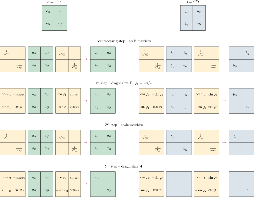
Figure 1 shows a schematic derivation of the two-sided Hari–Zimmermann transformations. Starting with a pair of symmetric matrices, where is positive definite, they are jointly transformed in four steps, i.e., twice by a diagonal scaling followed by a Jacobi rotation, after which both matrices become diagonal. The above formulas for follow by combining the last three steps into a convenient computation without the intermediate matrices.
2.2 Parallelization of the one-sided algorithm
The sequential one-sided algorithm in each step chooses a single pivot index pair, according to some criterion that is called a sequential Jacobi strategy. However, at most pivot column pairs of each matrix can be transformed concurrently if the indices in all index pairs are distinct.
In a parallel step a sequence of pivot index pairs, where , such that each index in the range from 1 to appears at most (and for even , exactly) once in the sequence, addresses pivot column pairs of and to be transformed—each pair by a separate, concurrent task. All permutations of a given are equivalent from the numerical point of view, since the resulting and are the same for every reordering of the sequence, and therefore any reordering represents the entire equivalence class.
For simplicity, a barrier is assumed between the successive parallel steps, i.e., all tasks of a step have to be completed before those of the following step are started.
A criterion to choose a pivot index pair sequence for each parallel step is called a parallel Jacobi strategy. Among the strategies that are simplest to compute are the ones that prescribe a pivot sequence for each step, until all index pairs are selected at least once. The choice of the steps is then periodically repeated. Let be the shortest such period. The first steps constitute the first sweep, the following steps the second sweep, and so on.
If in any sweep exactly different index pairs are chosen, such a strategy is called cyclic; otherwise, some index pairs are repeated in a sweep, and the strategy is called quasi-cyclic. For even , , and the equality holds if and only if the strategy is cyclic.
A strategy is defined for a fixed ; however, by a slight abuse of the usual terminology, a single principle by which the particular strategies are generated for some given matrix orders will simply be called a strategy kind, or even a strategy for short.
Based on the previous experience with the one-sided Jacobi-like algorithms, two parallel Jacobi strategy kinds have been selected for testing: the modified modulus (mm; see, e.g., Novaković and Singer (2011); Novaković et al. (2015)), quasi-cyclic with , and the generalized Mantharam–Eberlein (me; see Mantharam and Eberlein (1993); Novaković (2015)) cyclic one. Please see Figures 1 and 2 in the supplementary material, where a sweep of me and of mm, respectively, is shown two-sidedly on a matrix of order 32.
2.3 Blocking of the one-sided algorithm
Parallelization alone is not sufficient for achieving a decent performance of the algorithm on the modern architectures with multiple levels of the memory hierarchy.
The pointwise algorithm just described is therefore modified to work on the block columns of the matrices, instead of the columns proper. Each block column comprises an arbitrary but fixed number w, , of consecutive matrix columns. Instead of pivot submatrices of and , in the blocked algorithm pivot submatrices and are formed in the th (parallel or sequential) step by matrix multiplications,
where , , , , , and are the th and th block columns of , , and of width w.
Now, and can either be jointly diagonalized by a matrix , which leads to the full block (fb) algorithm Hari et al. (2014), as called in the context of the Jacobi methods, or their off-diagonal norms can be reduced by a sequence of congruences accumulated into , which is called the block-oriented (bo) algorithm Hari et al. (2010). The idea behind blocking is that , , and fit, by choosing w, into the small but fast cache memory (e.g., the shared memory of a GPU), to speed up the computation with them, as well as employing BLAS 3 (matrix multiplies) operations for the block column updates by afterwards:
The computation of in either fb or bo can be done by any convergent method; a two-sided method can be applied straightforwardly, but for the one-sided approach and have to be factorized first by, e.g., the Cholesky factorization
and then the same implicit Hari–Zimmermann method, pointwise or blocked, and in both cases, either parallel or sequential, can be recursively applied to and .
In the single-GPU algorithm, there is only one level of such a recursion, i.e., one level of blocking. The block, outer level of the algorithm and the pointwise, inner level do not need to employ the same strategy kind. Both levels, however, are parallel. The sweeps of the outer level are called the block (or outer) sweeps, and those of the inner level are called the pointwise (or inner) sweeps, which for fb are limited to 30 ( and are usually fully diagonalized in less than that number of sweeps), and for bo are limited to only one inner sweep. Apart from that, there is no other substantial difference between fb and bo.
The Cholesky factorization is not the only way to form and . One numerical stability improvement would be to use a diagonally pivoted version of the factorization instead Singer et al. (2012),
Another one would be to skip forming and explicitly by shortening the pivot block columns by the column-pivoted QR factorization directly Singer et al. (2020),
In both cases, let
where and are permutation matrices, while and are unitary and are not required to be stored, implicitly or explicitly, for any further computation.
However, the QR factorization (even without the column pivoting) of a pair of the tall and skinny block columns comes with a significant performance penalty on a GPU compared to the Cholesky factorization of a small, square pivot submatrix Novaković (2015), and the pivoted Cholesky factorization does not avoid a possibility of getting a severely ill-conditioned or by multiplying an ill-conditioned pair of block columns by itself. Both of these enhancements are therefore only mentioned here, with a performance comparison of the in-kernel QR factorizations versus the formation of the Grammian matrices and their Cholesky factorizations available in Appendix E. If the batched tall-and-skinny QR factorizations prove indispensable for a particularly ill-conditioned problem, cublasXgetrfBatched routine (with ) and Boukaram et al. (2018) could also be considered.
In the following, the blocked algorithm is assumed to form the pivot submatrices as
i.e., each one by a ZHERK (DSYRK in the real case) like operation in the BLAS terminology, and the non-pivoted Cholesky factorization is then used to obtain and , as demonstrated in Figure 2, where eight block columns of are depicted. The same illustration holds if is replaced by . The block columns of the same hue are paired together, according to the first step of the me strategy, giving four square blocks to be formed and factorized.
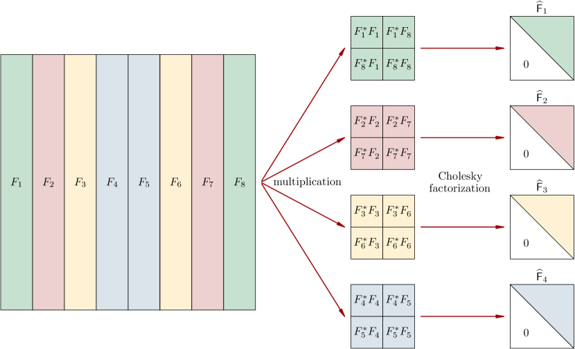
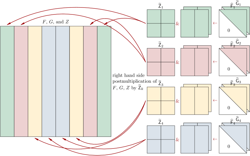
Figure 3 shows how each pair of the factors and is processed by the pointwise Hari–Zimmermann GSVD, leaving two matrices of the scaled left generalized singular vectors that are not used further, and a single matrix (rescaled, as noted in the following subsection 2.4) of the accumulated transformations. The block column pairs of , , and , with the physically disjoint but logically contiguous block columns, are then postmultiplied, each from the right by the corresponding , and replaced by the result.
2.4 Rescalings
Observe that is a product of several non-unitary matrices, elements of which can be larger than 1 by magnitude, so the norm of can build up significantly by such accumulation of the transformations. Also, if diagonalizes and , or reduces their off-diagonal norms, so does any matrix , where is a real, diagonal matrix with its diagonal elements positive and smaller than 1.
Let be such a matrix that reduces the norm of ,
where and stand for the th column of the final, transformed and , respectively, of which the latter has unit norm, and thus .
This is exactly the same scaling as it would be performed in the last, post-iterative phase of the algorithm,
except that and do not have to be rescaled and the norms of their columns do not have to be kept as they are all discarded immediately after has been computed.
Then, , is applied to the pivot block column pair of , , and instead of , and is considered embedded into in a similar way as would be in the pointwise case, i.e., starting from being , for each let
where the subscripting is to be interpreted as in Fortran.
To reduce the norm of the entire , a similar rescaling can be applied on , using the column norms of and , after each but the last block sweep. After the last block sweep, a rescaling of all three matrices (, , and ) is performed to obtain , , and , with the extraction of , , and .
2.5 Convergence
The inner level of the algorithm stops when there were no transformations, apart from the sorting permutations, applied in a sweep, or when the prescribed maximal number of sweeps has been reached. Then, the pivot block column pairs of , , and are updated concurrently for all by , which can be skipped for those where .
The same criterion could be used for the outer level, where the count of transformations applied in an outer sweep is a sum of all transformations applied in the inner level in all steps of the outer sweep. However, this criterion has to be relaxed Novaković (2015); Novaković et al. (2015), since the rounding errors in forming and factorizing the block pivot submatrices could spoil the attained numerical orthogonality of the original columns, and introduce a small number of unwarranted transformations that prevent the algorithm from detecting convergence even if it has in fact been reached.
Therefore, the transformations are divided in two classes: “big” and “small”. The latter are all where either:
-
C1.
, or
-
C2.
,
i.e., where is close to (a multiple of) identity, and the former are all other transformations. Note that neither definition of the small transformations implies that or are numerically equal to zero (and are usually not). Also, since tends to zero and therefore to one in the last sweeps of the algorithm, the first and the second definition should not differ significantly.
There are separate counters of the big transformations, and of all transformations applied in the inner level of the algorithm. The inner level still halts when there were no transformations of any class in a sweep, but the outer level stops when there were no big transformations applied in an outer sweeps (i.e., small transformations are allowed to occur but do not spoil the overall convergence). Such a heuristic criterion prevents in practice a long sequence of outer sweeps at the end of the algorithm, with only a few transformations close to identity in each.
2.6 Variants of the algorithm
To summarize the variants of the algorithm, see Table 1.
| ID | convergence | transformations | dot-products |
|---|---|---|---|
| 0 | criterion C1 | ( prescaled) | ordinary |
| 1 | criterion C1 | ( prescaled) | enhanced |
| 2 | criterion C1 | ( not scaled) | ordinary |
| 3 | criterion C1 | ( not scaled) | enhanced |
| 4 | criterion C2 | ( prescaled) | ordinary |
| 5 | criterion C2 | ( prescaled) | enhanced |
| 6 | criterion C2 | ( not scaled) | ordinary |
| 7 | criterion C2 | ( not scaled) | enhanced |
The first column, ID, sets a shorthand for the corresponding variant. The second column specifies a convergence criterion used. The third column distinguished between assuming the column norms of the second matrix to be unity, and rescaling of both matrices with each transformation. The fourth column relates to computing the dot-products the usual way, or by an enhanced, possibly more accurate procedure from Appendix A. Unless specified otherwise, the column sorting is employed in all cases. Thus, e.g., DHZ3-(mm-fb-me) refers to the double-precision real implicit blocked Hari–Zimmermann algorithm with ID equal to 3, using mm at the outer and me at the inner level of blocking of type fb. Similarly, ZHZ0-(me-bo-me) stands for the double-precision complex implicit blocked Hari–Zimmerman algorithm with ID equal to 0 (the “standard” variant), using me at both levels of blocking of type bo.
From now on, when a numeric variant ID is mentioned in the text, it is assumed that it should be looked up in Table 1.
3 The single-GPU implementation
In this section the single-GPU implementation of the complex and the real one-sided Hari–Zimmermann algorithms are described. The focus is on the complex algorithm, and the real one is commented on when substantially different. The target framework is CUDA C++ NVIDIA Corp. (2019) for the NVIDIA GPUs (Kepler series and newer), but also another general-purpose GPU programming environment with the analogous concepts and constructs could probably be used.
3.1 Data layout and transfer
Due to blocking employed by the algorithm, each matrix is viewed as column-striped, with the block columns containing consecutive columns each. To simplify the implementation, assume that is a multiple of 32, and let (so is even). If the assumption does not hold for the input, the matrices should then be bordered by appending columns to the right, and as many rows to the bottom. The elements , , …, in the columns newly added to the matrix should be set to unity, to avoid introducing zero columns, since it is essential for to be of full column rank. Other bordering elements should be set to zero, to prevent any transformation not implied by the original matrices from happening (see a bordering example in Novaković and Singer (2011)).
Another assumption, to simplify the loop unrolling in various parts of the code, is to have and as a multiple of 64. If it is not the case with the input, then, after a possible bordering as described above, rows of zeros should be appended to the bottom of the matrix .
3.1.1 The CPU and the GPU RAM layout and transfer
Data is laid out in the GPU RAM (also called “global memory” in the GPU context) in the following sequence:
after which follow the output-only vectors , , (with double-precision elements, each of length ), and (holding unsigned 8-byte integers, of length ). The rest of data is used both for input and output, i.e., the six double-precision matrices are constantly being read and overwritten within the GPU as the algorithm progresses. The matrices are loaded to the GPU at the beginning of the algorithm’s execution, if they are not already in place as a result of another computation, and optionally copied to the CPU at its end, as well as , , and .
In the pre- and post-processing stages on the CPU, input (, ) and output data ( in place of ; in place of ; and ), respectively, is repacked from (or to) the standard representation of complex matrices, in which the successive elements are complex numbers . Each double-precision matrix can therefore be loaded to, or copied from, the GPU with a single CUDA call.
This decision to keep all data in real-typed variables by splitting the real and the imaginary matrix parts and to perform the complex arithmetic manually is a design choice, not a necessity, since an implementation of the algorithm with the real and the imaginary parts interleaved in the customary way is also possible. There is no direct support for the standard C (with _Complex types) or C++ (with std::complex types) complex arithmetic in CUDA, so some non-standard approach has to be used anyway; e.g., the datatypes and the routines from the cuComplex.h header file, or those from the thrust library, or a custom implementation—possibly with a different memory layout—of complex numbers and the operations with them. The chosen, custom approach with the split data layout makes reading or writing only one (real or imaginary) component of the successive matrix elements straightforward, and such memory accesses can be contiguous.
In the auxiliary vector there are two counters, and , where is the index of a thread block in a grid of the main computational kernel. In the count of the “big” transformations, and in the count of all transformations applied in all kernel launches within a single block sweep are accumulated. At the beginning of each block sweep is zeroed out on the GPU, and is copied to a CPU vector at the end of the sweep.
3.1.2 The shared memory layout
For each thread block, the non-constant, non-register data (comprising three complex matrices: , , and ) for the main computational kernel is laid out in the shared memory as:
Each double-precision matrix is square, of order , with the elements stored in Fortran array order, for a total shared memory requirement of for a thread block. The shared memory is configured with 8-byte-wide banks. No other kernel requires any shared memory.
Let stand for the contiguous memory space occupied by and ; for and ; for and ; and for and , as the real and the imaginary parts of and matrices that share the same storage with , , and . Such overlapping of data is necessary for the formation of and from the block columns of and , respectively, as described below. Also, let stand for , , ; and for , , .
The real case
In the real Hari–Zimmermann algorithm matrices do not exist, so repacking of the input and the output data does not happen. The other properties of two data layouts still hold. The shared memory requirements are half of those for the complex algorithm, i.e., .
3.1.3 The constant memory layout
The constant memory on the GPU holds the pointers to the matrices and the vectors described above, with their dimensions, to avoid sending them as parameters in each kernel call. The Jacobi strategy table for the first, pointwise level of the algorithm is also stored in the constant memory, since it does not depend on the actual input data.
The strategy table contains 31 (or 32) rows, same as the number of steps of a chosen (quasi-)cyclic parallel strategy. Each row is an array of 16 index pairs , with , where no two indices in a row are the same. A pair of such indices addresses a pair of columns of the matrices and to be transformed concurrently with all other column pairs in the step.
3.1.4 Constants in the global memory
The Jacobi strategy table for the second, block level of the algorithm might not fit in the constant memory for the large , so it has to be stored in the global memory in such a case. It is similarly formatted as the table for the pointwise level, but with (or ) rows, each with index pairs. Here, a pair , with , addresses a pair of block columns of the matrices and . No two indices in a row are the same, i.e., every integer between 0 and appears exactly once in a row. Each row encodes a step of the chosen block level (quasi-)cyclic parallel strategy, which does not have to be of the same kind as the one chosen for the pointwise level.
3.2 Arithmetic operations
Since the data is held in the real-valued arrays only, the complex arithmetic is performed manually, computing the real and the imaginary parts of the result separately, rather than assembling the complex operands in the CUDA format each time an operation has to be performed, and disassembling the result when it has to be stored back in memory.
3.2.1 Complex arithmetic
The arithmetic operations on complex numbers needed by the algorithm are addition, subtraction, negation, complex conjugation, multiplication by a complex or a real number (or an inverse of the latter), and taking the absolute value. Only , , and an FMA-like operation (a complex multiplication and an addition fused) require special attention, while the rest are trivial to express by the real arithmetic directly in the code.
The absolute value is obtained as , without undue overflow. Still, it is possible that overflows when at least one component of is close enough by magnitude to the largest representable finite double-precision number, but such a problem can be mitigated by a joint downscaling of two matrices under transformation. For example, a scaling by would suffice, and would also keep the significand intact for all normalized (i.e., finite non-subnormal) numbers. Such rescaling has not been implemented, though it would not be overwhelmingly hard to apply the rescaling and restart the computation if any thread detects that its operation has overflowed, and makes that known to other threads in a block by a subsequent __syncthreads_count CUDA primitive invoked with a Boolean value indicating the presence of an overflow.
For multiplication, an inlineable routine (zmul) computes and returns the result via two output-only arguments, referring to and . With the CUDA FMA intrinsic __fma_rn it holds
computed in a way that requires three floating-point operations but two roundings only. Note that the operations are ordered arbitrarily, thus zmul could also be realized by multiplying the real parts of the factors first. is obtained by
where only two instead of three floating-point operations are required, with two roundings, and the choice of the real product arguments is arbitrary. In total, five operations (of which the negation is trivial) instead of six are needed.
The FMA-like operation is modeled after the CUDA one in the cuComplex.h header. Let . Then, zfma routine requires 3 operations with 2 roundings for
and 2 operations with 2 roundings for
It holds for all and .
3.2.2 Real arithmetic
The real arithmetic uses operations with the accuracy guarantees mandated by the IEEE 754 standard for floating-point arithmetic in rounding to nearest (ties to even) mode, except in the optional enhanced dot-product computation, where rounding to is also employed, as described in Appendix A.
A correctly rounded (i.e., with the relative error of no more than half ulp) double-precision device function, provided by Norbert Juffa in private communication, that improves the accuracy of the CUDA math library routine of the same name (let it be referred to by when a need arises to disambiguate between the two, and by when either is acceptable), is called wherever such an expression has to be computed.
3.2.3 Reproducibility
In both the real and the complex code function is expected, but not extensively verified, to be correctly rounded and thus reproducible. Reproducibility of the results is guaranteed for the complex code as long as it is for the function in all CUDA versions and on all GPUs under consideration. All other floating-point arithmetic operations with rounding (i.e., not including the comparisons and the negations) are expressed in the terms of the seven double precision CUDA intrinsics.
3.2.4 Integer arithmetic
To keep the memory requirements low, the pointwise level indices in the strategy table are stored as unsigned 1-byte integers, while the block level indices occupy 2 bytes each (i.e., , what is enough to exceed the RAM sizes of the present-day GPUs).
For dimensioning and indexing purposes the unsigned 4-byte integers (after a possible promotion) are used, since their range allows for addressing up to of double-precision floating-point data, which is twice the quantity of GPU RAM available on the testing hardware. However, 8-byte integers should be used instead if the future GPUs provide more memory than this limit.
Although Fortran array order is assumed throughout the paper and the code, the indices on a GPU are zero-based. The CUDA thread (block) indices blockIdx.x, threadIdx.x, and threadIdx.y are shortened as , , and , respectively.
3.3 Initialization of with optional rescaling of and
Here, initFGZ, the first of three computational kernels, is described. Its purpose is to initialize the matrix , having been zeroed out after allocation, to , a diagonal matrix such that , and to rescale and to and , by multiplying the elements of each column of the matrices by in the variants 0, 1, 4, and 5. Else, in other variants, .
The kernel is launched once, before the iterative phase of the algorithm, with a one-dimensional grid of thread blocks, each of which is also one-dimensional, with 64 threads (two warps of 32 consecutive-numbered threads).
A warp is in charge of one column of , , and , i.e., its threads access only the elements of that column , where
A warp reads 32 consecutive elements of and at a time. Each of its threads updates its register-stored partial sums
using one FMA operation for each update, and this is repeated by going to rows until . Initially, and . After passing through the entire column, those partial sums are added to obtain . Then, are summed and the result is distributed across the warp by a warp-shuffling NVIDIA Corp. (2019) sum-reduction, described in Appendix C, yielding the sum of squares of the magnitudes of the elements in the column, i.e., .
Such a computation occurs in the variants 0 and 4, while in the variants 1 and 5 the enhanced dot-product computation as in Appendix A updates the per-thread, register-stored partial sums , , , . After a pass over the column completes, are formed according to the rules of Appendix A and summed as above.
Either way, is then computed, and the th columns of and are scaled by in a loop similar to the one described above, i.e., for in steps of 32 while ,
and then the same scaling is performed on , with .
Finally, is written to by the lowest-numbered thread in a warp, i.e., , where is an index making a physical column treated as a logical column . In the single-GPU case, . In the variants 2, 3, 6, and 7, is set to 1 and no other processing occurs.
This and any other computation of the Frobenius norm of a vector via the sum of squares of its elements could overflow even if the result itself would not. See (Novaković, 2015, Appendix A) for one of several possible remedies.
3.4 Rescaling of and extraction of , , , , and
After each block sweep, another kernel, rescale, is called, with a Boolean flag f indicating whether it is the last sweep.
If f is false, only is rescaled according to the rules of subsection 2.4, and otherwise the full results of the GSVD computation (, , , , and ) are produced.
The kernel’s grid is identical, and the operation very similar to initFGZ. First, is computed, and if non-unity and f, is scaled by . If f, . Then, is computed, and if non-unity and f, is scaled by , as well as to obtain ; else, if f, .
Then , , and . If , is scaled by , as well as and to obtain and ; else, and .
Finally, if f, , , and are written to the GPU RAM by a thread . All variables indexed by above are per-thread and register-stored, unless a register spill occurs.
3.5 The main computational kernel
The main kernel comes in bstep1s and bstep1n versions, where the former is the default one, with the column sorting, while the latter is a non-sorting version.
The kernel is called once per a block step. Each such call constitutes the entire block step, and it cannot run concurrently with any other GPU part of the algorithm since it can update almost the whole allocated GPU memory.
The kernel’s grid is one-dimensional, with two-dimensional thread blocks, each of them having threads. A thread block in the block step is in charge of one pivot block column pair, , of , , and , where is for the me or for the mm strategy kind.
The computational subphases of bstep1(s/n)(),
-
1.
formation of and in the shared memory,
-
2.
the Cholesky factorizations of and as and , respectively,
-
3.
the pointwise implicit Hari–Zimmermann algorithm on the matrix pair , yielding ,
-
4.
postmultiplication of the pair of pivot block columns of , , and by ,
are all fused into a single kernel to effortlessly preserve the contents of the shared memory between them.
All the required matrix algebra routines have been written as device functions with the semantics similar to, but different from the standard BLAS, due to the data distribution and the memory constraints. For example, a single call of the BLAS-compatible ZHERK (or DSYRK in the real case) operation for the subphase 1 is not possible, since the two pivot block columns do not have to be adjacent in the global memory. The subphase 3 cannot use a single standard ZGEMM (or DGEMM) call for the same reason, but also because the block columns have to be overwritten in-place to avoid introducing any work arrays.
Since no two pivot block index pairs share an index, all thread blocks can be executed concurrently without any interdependencies or data races. Due to the shared memory requirement and a high thread count, it is not possible that more than two (or, in the real case, four) thread blocks could share a single GPU multiprocessor (an SM for short, which cannot have more than 2048 threads resident at present). On a Maxwell GPU, the profiler reports occupancy of 25% for the real and the complex bstep1s, i.e., at most one thread block is active on an SM at any time. That can be attributed to a huge register pressure, since 128 registers per thread are used for the main kernel (in the variant 0), with a significant amount of spillage, thus completely exhausting the SM’s register file. Should more than registers be available per SM, it might be possible to achieve a higher occupancy.
Therefore, for the matrices large enough, only a fraction of all thread blocks in the grid can execute at the same time on a GPU. It is a presumption (but not a requirement) that the CUDA runtime shall schedule a thread block for execution at an early opportunity after a running one terminates, thereby keeping the GPU busy despite of the possible execution time variations (i.e., the number of the inner sweeps and the transformations required) among the thread blocks, especially in the fb case.
Note that addresses a warp, , and , , denotes a lane (a thread) within the warp. Throughout a thread block, each warp is in charge of two “ordinary” (i.e., not block) columns, in the global or in the shared memory, but of which two varies between and within the subphases.
3.5.1 Subphase 1 (two ZHERK or DSYRK like operations)
The task of this subphase is to form and then in the shared memory, occupying (and ), and (and ), respectively, by a single pass through the pivot block columns of and . The resulting matrices are Hermitian in theory, but unlike in BLAS, both the strictly lower and the strictly upper triangle of each matrix are explicitly computed, even though only the lower triangle is read in the subphase 2, thus avoiding a possible issue with one triangle not being the exact transpose-conjugate of the other numerically.
A warp indexed by is assigned two column indices, and , in the range of the first and the second pivot block column, respectively, as
Each thread holds four register-stored variables,
initially set to zero, that hold the real (first two) and the imaginary (last two) parts of two (partial) dot-products of the columns of and, in the second instance, of , where .
In a loop over , starting from and terminating when , with , in each step two consecutive chunks of 32 rows (i.e., 64 rows) of the columns and are read from and into and . Each lane reads an element from the global memory and writes it into the shared memory, both in the coalesced manner, four times per chunk. The elements of the column are stored into the th column, and those of the column are stored into the th column of the shared memory buffer. The elements of the first chunk are stored into the th row, and of the second chunk into the th row of the buffer. The thread block is then synchronized, to complete filling the buffer by all warps.
An unrolled inner loop over , , followed by a synchronization call, updates the local partial dot-products.
For each , let , and
Two fused multiply-add operations perform the updates
The first updates constitute a computation of the dot-product of th and th column of and updating the partial sum with it, while the second ones form the dot-product of the th and th column and update with it. Note that all the rows of the buffer are read exactly once, albeit in the modular (circular) fashion throughout the loop, with the different starting offsets in each column to minimize the shared memory bank conflicts.
When the outer loop over terminates, and are stored into at the corresponding indices, and a synchronization barrier is reached, thus finalizing the formation of . The same procedure is repeated with instead of to obtain , substituting and for and , respectively, in the procedure described above. Note that could (however, unclear if it should) be used instead of , i.e., three chunks instead of two would be read into the buffer and the dot-products of the columns of length 96 instead of 64 would be computed. That would not be possible, though, for , since , once formed, must not be overwritten until the next subphase.
In Figure 4 the arguments A0D, A0J, A1D, A1J, AD, and AJ stand for the real and the imaginary planes of the th and the th columns of , and for and , respectively, in the first call of the device function. The same holds for and in the second call. The indices x, y0, and y1 correspond to , , and , respectively, while m is the number of rows of or .
// F??(A, i, j) = A[?? * j + i] (??=32|64)
// cuD: real, cuJ: imaginary part (double)
__device__ __forceinline__ void zAhA
(const cuD *const __restrict__ A0D,
 const cuJ *const __restrict__ A0J,
 const cuD *const __restrict__ A1D,
 const cuJ *const __restrict__ A1J,
 volatile cuD *const __restrict__ AD,
 volatile cuJ *const __restrict__ AJ,
 const unsigned m, const unsigned x,
 const unsigned y0, const unsigned y1)
{
  cuD y0xD = 0.0, y1xD = 0.0;
  cuJ y0xJ = 0.0, y1xJ = 0.0;
  const unsigned x32 = x + 32u;

  for (unsigned i = x; i < m; i += 32u) {
    // read the 1st 32 x 32 chunk from RAM
    F64(AD, x, y0) = A0D[i];
    F64(AJ, x, y0) = A0J[i];
    F64(AD, x, y1) = A1D[i];
    F64(AJ, x, y1) = A1J[i];

    i += 32u;
    // read the 2nd 32 x 32 chunk from RAM
    F64(AD, x32, y0) = A0D[i];
    F64(AJ, x32, y0) = A0J[i];
    F64(AD, x32, y1) = A1D[i];
    F64(AJ, x32, y1) = A1J[i];
    __syncthreads();

    #pragma unroll
    for (unsigned j = 0u; j < 64u; ++j) {
      const unsigned x_64 =
        (x + j) & 0x3Fu; // (x + j) % 64u
      const cuD _x_hD =  F64(AD, x_64, x);
      const cuJ _x_hJ = -F64(AJ, x_64, x);
      const cuD _y0_D =  F64(AD, x_64, y0);
      const cuJ _y0_J =  F64(AJ, x_64, y0);
      const cuD _y1_D =  F64(AD, x_64, y1);
      const cuJ _y1_J =  F64(AJ, x_64, y1);
      // [complex] y0x = _x_h * _y0_ + y0x
      Zfma(y0xD, y0xJ, _x_hD, _x_hJ,
        _y0_D, _y0_J, y0xD, y0xJ);
      // [complex] y1x = _x_h * _y1_ + y1x
      Zfma(y1xD, y1xJ, _x_hD, _x_hJ,
        _y1_D, _y1_J, y1xD, y1xJ);
    }
    __syncthreads();
  }

  // A^H * A stored into the shared memory
  F32(AD, x, y0) = y0xD;
  F32(AJ, x, y0) = y0xJ;
  F32(AD, x, y1) = y1xD;
  F32(AJ, x, y1) = y1xJ;
  __syncthreads();
}
3.5.2 Subphase 2 (two ZPOTRF or DPOTRF like operations)
The Cholesky factorization of or consists of two similar, unrolled loops over . The matrix (in Fortran array order) is accessed and transformed columnwise to avoid the shared memory bank conflicts, but then a transpose-conjugate operation must follow on the computed lower triangular factor to obtain the corresponding upper triangular one. Along with the transposition-conjugation, the strictly lower triangle is zeroed-out, since the following subphase makes no assumptions about the triangularity of the initial matrices.
The first loop iterates over . First, the th diagonal element of , , is read (the imaginary part is assumed to be zero) if and (i.e., in the threads of the th warp which correspond to the lower triangle, called the “active” threads), and the thread block is then synchronized.
The active threads then scale the th column below the diagonal, each thread the real and the imaginary part of its element in the th row, by , while the diagonal is set to , and the thread block is then synchronized.
Next, the columns to the right of the th have to be updated, with all warps (but not all their threads) participating in the update. Let . Then, if ,
and the thread block is synchronized. However, this only updates the columns from to . The same update has to be performed with instead of , i.e., if (which also ensures that ),
and another thread synchronization occurs.
The second loop over is identical to the first one, except that is used instead of and the second updates (of the th columns) are not needed since .
The ensuing transpose-conjugate with zeroing-out of the strictly lower triangle is performed by reading and into the register of the th thread if and , respectively (i.e., the indices belong to the lower triangle of ). Otherwise, those registers are set to 0. After negating the imaginary parts in the former case, the values are written to and , respectively, unfortunately requiring the shared memory bank conflicts, and the thread block is synchronized, yielding . The same procedure is then repeated with instead of , yielding .
3.5.3 Subphase 3 (the pointwise one-sided algorithm)
The pointwise implicit Hari–Zimmermann algorithm, described in section 2, subsections 2.1, 2.2, and the relevant parts of subsections 2.4 and 2.5, is implemented as follows.
The th warp transforms the pairs of columns of , , and in each inner step . Let , since the me strategy is used exclusively at the inner level in the tests. Each of the three pivot pairs comprise the columns indexed by and , where the indices are read from the th row of the inner strategy table at the position . Within a warp, the th thread is responsible for the elements in the th row of those columns.
First, is initialized similarly to the procedure described in subsection 3.3, but on the shared memory level. In the variants 2, 3, 6, and 7, the diagonal of is set to unity, and the rest to zero, by the threads in charge of those elements. In the variants 0 and 4, the sum of squares of the magnitudes of the elements of the columns , i.e., , where and , is computed by a sum-reduction as in Appendix C. The thread block is then synchronized. For each of the two indices , is set to zero, as well as , except when , where if , and one otherwise. The columns and are scaled by if it is not unity, and the thread block is synchronized. The similar procedure is applied in the variants 1 and 5, except that the partial sums of squares are computed as in Appendix A (see subsection 3.3), and summed by a routine from Appendix C.
Having thus obtained , , and , the iterative part of the algorithm starts, with at most 30 (fb) or 1 (bo) inner sweeps. At the start of each sweep two per-sweep counters, of the “big” () and of all () transformations applied, are reset to zero. The counters are kept in each thread, but their values are synchronized across all threads in a thread block.
In the step and the warp , let and . The elements of the three pivot column pairs are loaded into the registers by each thread reading its row from the shared memory, after which the thread block is synchronized. For each original element, there are two variables for its real and imaginary parts, and two more variables to hold the value of the new element after transformation, since the old value is used twice in computing the new one and thus cannot be overwritten. For example, has as its counterpart.
The pivot submatrices and are then formed. The diagonal elements are obtained by computing the squares of the column norms as above, and the off-diagonal ones are given by the dot-products, either ordinary (i.e., by sum-reducing the real and the imaginary parts of the products of an element of the th column conjugated and the corresponding element of the th column) or enhanced (as in Appendix A) ones.
However, and thus obtained have to be multiplied by from the left and right in the variants 2, 3, 6, and 7 to get and . If , then , , and , are scaled by ; otherwise, , as it is in the variants 0, 1, 4, and 5. If , then , , and , are scaled by ; otherwise, .
All threads in a warp now have the elements of the pivot submatrices held in their register-stored variables, and the elements’ values are identical across the warp. Therefore, the subsequent computation of on a per-thread basis also has to produce the same transformation across the warp.
First it has to be established whether a transformation is warranted. If the relative orthogonality criterion is satisfied, is set to zero, else to one. All threads in a thread block agree if there is some computational work (apart from merely the optional column sorting) to be done in the current step by uniformly incrementing ,
by the number of the thread block’s warps with the non-trivial transformations to be applied.
If and , then and , where and in bstep1s. Then, the values of the new variables are stored in the shared memory. When in bstep1n, or in bstep1s and , the new variables take the value of the corresponding old ones, i.e., no column swapping occurs.
Otherwise, for , is computed according to a procedure described either in subsection 2.1.1 for the complex, or in subsection 2.1.2 for the real case. Then, it is established whether the criterion C1 (for the variants 0, 1, 2, and 3) or the criterion C2 (for the variants 4, 5, 6, and 7) indicates that the transformation is “small”. If so, ; else, .
If , the first row of is scaled by . If , the second row of is scaled by . Now the completed transformation has to be applied to the pivot columns:
where . If one or both scaled cosines lying on the diagonal of are equal to one, the transformation can be (and is) simplified by removing the corresponding multiplications without numerically affecting the result.
In bstep1s, to determine if the column swap is required, the squares of the norms of the transformed columns of are computed as the sum-reduced sums of squares of the magnitudes of the new () elements, depending on the variant. Those two values are however not stored for the next step, because that would require an additional shared memory workspace that might not be available on all supported architectures.
In the real case it is easy to compute instead the transformed diagonal elements of the first pivot submatrix directly Novaković et al. (2015):
and to swap the th and the th column when .
If the norm of the th column is smaller than the norm of the th column, then the values of and are swapped via an intermediary variable. Else, or in bstep1n, no swaps occur. The values of the new variables are then stored in the shared memory, and is uniformly incremented across the thread block,
The th step is now complete.
At the end of a sweep, if , the loop is terminated. Else, the counters and , set at the start of this subphase to zero, are incremented by and , respectively.
The same rescaling as in subsection 3.4 with f=false, but performed on the shared memory, yields . Using the last values of and , the squares of the norms of the th column of and , respectively, are computed. Then, is read (or its last value is used), scaled by , stored, and the thread block is synchronized. The same procedure is repeated with instead of , giving .
A thread with stores and into as
and finally the thread block is synchronized.
3.5.4 Subphase 4 (three postmultiplications)
In this subphase the pivot block columns of , , and are multiplied by and overwritten by the respective results.
Each multiplication of a pair of pivot block columns (residing in the global memory) by (residing in the shared memory in ) and the following update are performed by a single pass over (i.e., a single read from and a single write to) the block columns, using the Cannon-like algorithm Cannon (1969) for parallel multiplication of two square matrices.
Reading the chunks of a block column pair from the global memory is identical to the one from the subphase 1 in subsection 3.5.1, except that in each iteration of the outer loop (over ) only one chunk is read to , instead of two (which would also be a possibility). The number of loop iterations (in parenthesis) depends on the number of rows of (), (), and (). Here, is when updating and , and when updating . The thread block is then synchronized.
The per-thread variables to hold the product of the current chunk with are set to zero. Each thread is in charge of forming the elements with indices and of the product .
The initial skews are defined as and . Then, in each iteration of the unrolled inner loop over the local elements of are updated,
and and are cyclically shifted as and . When the inner loop terminates, the thread block is synchronized.
The local values of now have to be written back to the global memory, where overwrites , while overwrites , for being one of . The thread block is then synchronized and the next outer iteration, if any are left, follows.
This procedure is called thrice to update , and , after which the kernel execution (i.e., the th outer step) terminates and the control returns to the CPU.
Figure 5 shows the postmultiplication device function, where the arguments A0D, A0J, A1D, and A1J have the same meaning as in Figure 4, but the columns of are also expected. A shared memory buffer, in which the chunks of a block column pair are loaded and packed, is pointed to by AD and AJ, while BD and BJ point to the accumulated transformation matrix from the subphase 3, by which the postmultiplication has to take place. The product of matrices A and B overwrites the respective chunk of the original block columns before another chunk is loaded.
__device__ __forceinline__ void zPostMult
(cuD *const __restrict__ A0D,
 cuJ *const __restrict__ A0J,
 cuD *const __restrict__ A1D,
 cuJ *const __restrict__ A1J,
 volatile cuD *const __restrict__ AD,
 volatile cuJ *const __restrict__ AJ,
 volatile const cuD *const __restrict__ BD,
 volatile const cuJ *const __restrict__ BJ,
 const unsigned x, const unsigned y0,
 const unsigned y1, const unsigned m)
{
  // Cannon-like C = A * B
  for (unsigned i = x; i < m; i += 32u) {
    F32(AD, x, y0) = A0D[i];
    F32(AJ, x, y0) = A0J[i];
    F32(AD, x, y1) = A1D[i];
    F32(AJ, x, y1) = A1J[i];
    __syncthreads();

    cuD Cxy0D = 0.0, Cxy1D = 0.0;
    cuJ Cxy0J = 0.0, Cxy1J = 0.0;
    unsigned // skew (mod 32)
      p0 = ((y0 + x) & 0x1Fu),
      p1 = ((y1 + x) & 0x1Fu);

    // multiply and cyclic shift (mod 32)
    #pragma unroll
    for (unsigned k = 0u; k < 32u; ++k) {
      Zfma(Cxy0D, Cxy0J,
        F32(AD, x, p0), F32(AJ, x, p0),
        F32(BD, p0, y0), F32(BJ, p0, y0),
        Cxy0D, Cxy0J);
      Zfma(Cxy1D, Cxy1J,
        F32(AD, x, p1), F32(AJ, x, p1),
        F32(BD, p1, y1), F32(BJ, p1, y1),
        Cxy1D, Cxy1J);
      p0 = (p0 + 1u) & 0x1Fu;
      p1 = (p1 + 1u) & 0x1Fu;
    }
    __syncthreads();

    A0D[i] = Cxy0D; A0J[i] = Cxy0J;
    A1D[i] = Cxy1D; A1J[i] = Cxy1J;
    __syncthreads();
  }
}
3.5.5 Dataflow and the shared memory perspective
In Figure 6 the subphases in the simpler, real case are summarized from a perspective of the data in the shared memory and the transformations that it undergoes.
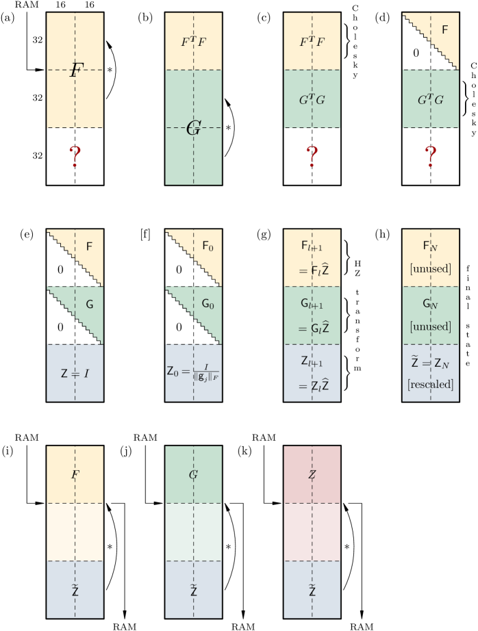
The subfigures (a–b) show the chunks of data coming from the global memory to form and . Two Cholesky factorizations are shown in the subfigures (c–d), after which the subfigures (e–h) correspond to the subphase 3. The subfigure [f] shows the optional (depending on the variant) prescaling of and . The final three subfigures, (i–k), show the three postmultiplications taking place, with a chunk of data read from and written to the global memory. Two different hues of the first and the middle parts of the shared memory depiction indicate that the chunks with 64 instead of 32 rows might be used there.
3.6 The CPU part of the algorithm
Algorithm 1 summarizes the CPU-side actions with a single GPU.
The same routine is called within the multi-GPU algorithm, except for allowing to be a parameter (not the constant as it is assumed here), a variation of the final rescaling of , and some differences regarding the initFGZ call, described in subsections 3.3 and 4.2. The copy-ins and copy-outs of the majority of data, as well as the initialization of the constant memory, are left out from Algorithm 1 but are included in the single-GPU timing in subsection 5.
Apart from the copy-ins, copy-outs, and zeroings of data, there is no scope for using more than one CUDA stream. All GPU operations can be performed in any predefined stream s (e.g., in the default one if no other has been explicitly chosen). Also, as no GPU computation, except the fast rescale, can be overlapped with any CPU task, the execution time of the algorithm depends almost solely on the GPU performance and the time required to set up a kernel call.
Each kernel invocation and each sequence of memory copy/set operations is followed in the testing code by a (generally redundant, except where noted in Algorithm 1) cudaStreamSynchronize call on the chosen stream s, to keep the CPU-side timing consistent (but maybe higher than it is necessary).
Except the reductions of and for very large matrices, no other part of the algorithm might benefit from being executed multi-threadedly on the CPU. From the CPU perspective, the algorithm is therefore purely sequential.
Note that the algorithm stops when , i.e., when no big transformations occurred in an outer sweep. The “global” counts and of all and of big transformations applied during the execution of Algorithm 1 are only informative here, but they are consulted in the multi-GPU algorithm’s stopping criterion.
4 The multi-GPU implementation
When the input data is larger than the available RAM on a single GPU, it is necessary to either split the workload among the several GPUs, or resort to some out-of-core technique for swapping the parts of data in and out of the GPU as the computation progresses. Here, only the former approach is followed, since it is simpler, more efficient and widely applicable now when the multi-GPU installations are becoming ubiquitous. In the case when not enough GPUs are available for the input data to be distributed across them, see an outline of a possible out-of-core single-GPU algorithm in Appendix B.
There is no single, best and straightforward way of generalizing a single-GPU algorithm to multiple GPUs. For the (ordinary and hyperbolic) SVD, the approach in Novaković (2015) was to distribute the matrix over the GPUs, shorten the assigned part of the matrix (the Grammian formation being done by cuBLAS, and the ensuing Cholesky factorization by MAGMA Tomov et al. (2010)), run the single-GPU algorithm on the shortened part, update the original (non-shortened) columns, and redistribute the parts. Despite its decent performance, such a three-level algorithm suffered from the increased memory usage and some numerical difficulties, both with the stopping criteria and with the relative accuracy obtained.
A different approach is taken here, to achieve the optimal GPU and CPU memory usage (without any work arrays) and a better accuracy, but with a possible performance penalty induced by transforming the tall and skinny parts of the matrices directly, without any shortening. As no floating-point computation is performed on the CPU, while the GPU computation still does not rely on any numerical libraries, it is guaranteed that the results stay bitwise identical in the repeated runs over the same input data with the same parameters and the same number of GPUs.
4.1 Algorithm setup
In this subsection the multi-GPU computational environment, the input and the output data distribution across the CPUs and the GPUs, the communication-aware Jacobi strategies, and the algorithm’s initialization are explained.
4.1.1 MPI environment
Unlike in Novaković (2015), where the multiple GPUs were assumed to belong to the same node, and thus a separate CPU thread of a single process could be dedicated for driving the computation on each GPU, here a more flexible solution has been chosen, by assigning to a GPU a single-threaded MPI Message Passing Interface Forum (2015) process. The GPUs can thus be selected from any number of nodes, with a different number of them on each node. Also, the GPUs are not required to be architecturally identical or even similar across the processes in an MPI job, as long as they all have enough RAM available.
The count of GPUs, and thus the governing MPI processes (), for the multi-GPU algorithm is not constrained in principle, save for being at least two (otherwise, the single-GPU algorithm is sufficient), and small enough so that at least two (but for the reasons of performance, a multiple of 32) columns of each matrix are available to each process, when the matrices are divided among them columnwise, as described below. The upper bound on the number of GPUs is a tunable parameter in the code, while the MPI implementation might have its own limit on the number of processes in a job.
The MPI processes need not be arranged in any special topology. Only the predefined MPI_COMM_WORLD communicator is used. A GPU and its governing process are jointly referred to by the process’ rank () in that communicator.
It is assumed that the MPI distribution is CUDA-aware in a sense that sending data from the GPU RAM of one process and receiving it in the CPU RAM of another (including the same) process is possible with the standard MPI point-to-point communication routines (i.e., no manual CPU buffering of the GPU data is necessary).
Also, the number of elements of each local submatrix has to be at most INT_MAX, which at present is the upper limit on the count of elements that can be transferred in a single MPI operation Hammond et al. (2014). That limit is easily circumvented by transferring the data in several smaller chunks, but such chunking has not been implemented since it was not needed for the amount of RAM () of the GPUs used for testing. That issue will have to be addressed for the future GPUs.
4.1.2 Data distribution
The matrices , , and , and the vectors , , and , are assumed to always stay distributed among the MPI processes, i.e., at no moment they are required to be present in entirety in any subset of the processes. The amount of the CPU and the GPU memory required is identical (i.e., not depending on ), constant throughout the computation, and derivable in advance from , , , and for all processes.
If or , the matrices , , and are bordered as described in subsection 3.1, but requiring that the enlarged satisfy . Similarly, the bordering is required if or .
The columns of the bordered matrices can be distributed evenly among the processes, such that each process is assigned columns. Let consecutive columns of an entire matrix be called a stripe, to avoid reusing the term “block column”. Then, a process holds two, not necessarily consecutive, stripes of each matrix, logically separate but with their real parts physically joined in the same memory allocation, as well as their imaginary parts. The dimensions of two joined stripes, one following the other in the Fortran array order, of (), (), and (), fit the requirements for the input data of the single-GPU algorithm.
The CPU RAM of the th process thus holds two joined stripes in , , , , , and allocations. The same memory arrangement is present in the GPU RAM, which holds the same stripes undergoing the transformations and joined in the allocations , , , , , and . The first stripe within an allocation is denoted by the index , and the second one by the index ; e.g., is the second stripe in .
A similar distribution is in place for , , and , where each process holds , , and in the CPU RAM, and , , and in the GPU RAM, where each allocation is of length and is unused in the algorithm until after the last step. Each process also has its convergence vectors and , of length , in the CPU and in the GPU RAM, respectively.
4.1.3 Communication-aware Jacobi strategies
The parallel Jacobi strategies, as defined in subsection 2.2, do not contain any explicit information on how to progress from one step to another by exchanging the pivot (block) columns among the tasks in a distributed memory environment. However, such a communication pattern can be easily retrieved by looking at each two successive steps, and , and for each task in the th step finding the tasks and in the th step that are to hold either th or th (block) column.
Therefore, given either me or mm strategy table for the order (with the stripes seen as the block columns), each process independently computes and encodes the strategy’s communication pattern before the start of the algorithm. Such a computation requires comparisons, but since is a small number an unacceptable overhead is not incurred. The computation can be (but it has not been) parallelized on a CPU, e.g., by turning the outer loop over into a parallel one. The multi-GPU algorithm then references the following encoded mapping when progressing from one step to the next.
After each outermost (multi-GPU) step of the algorithm, the first of each two joined stripes on the th GPU has to be transferred to either the first or the second stripe on the th CPU, for some . Similarly, the second stripe on the th GPU has to be transferred to either the first or the second stripe on the th CPU, for some , establishing a mapping
where , , while and are indices of the first and the second stripe in the entire matrix, , and are the MPI ranks. If the th stripe globally (i.e., the first locally) has to be transferred to the first stripe in the th process, that is encoded as , else the second stripe of the target is encoded as . Similarly, if the th stripe globally (i.e., the second locally) has to be transferred to the first stripe in the th process, that is encoded as , else the second stripe of the target is encoded as . Adding to the rank ensures that the rank can be encoded as either or .
The number of steps in a sweep, denoted by , is for me, and for mm. The strategy mapping, once computed, can be reused for multiple runs of the algorithm, as long as the strategy kind, (after bordering), and do not change between the runs.
4.1.4 Algorithm initialization
First, the CPU memory is allocated in each process, and the data is loaded (e.g., from a file), assuming , i.e., the th process contains the th and th stripes of , , and .
Then, the device memory is allocated, if it is not already available, and an MPI barrier is reached. Timing of the algorithm includes everything that occurs from this barrier on, except the optional deallocation of the device memory.
The constant memory on each GPU is set up, and the stripes are copied to the device (global) memory, all of which could be done asynchronously. The involved stream(s) are then synchronized, depending on the way the copies have been performed.
It remains to be decided how many sweeps in Algorithm 1 to allow. As with the pointwise level, there are two obvious choices: either some reasonably large number, e.g., (as in fb), or (as in bo). Now a variant of the multi-GPU algorithm is specified by the selected variant of the single-GPU algorithm, with the outermost strategy and the choice of added; e.g., ZHZ0-(me-bo, me-fb-me) for me and , respectively, using ZHZ0-(me-fb-me) at the single-GPU level.
As shown in subsection 5.3.2, the imbalance of the computational time each GPU requires with fb (i.e., one GPU may need more sweeps in Algorithm 1 than another to reach convergence within an outermost step) is significantly detrimental to the overall performance—contrary to the single-GPU case (see subsection 3.5). Unlike there, where such imbalance between the thread blocks’ sweep counts is offset by a large number of thread blocks to be scheduled on a small number of multiprocessors, here in the multi-GPU case there is a one-to-one correspondence between the number of tasks to perform and the number of execution units (GPUs) to perform them, so the time required for an outermost step depends on the slowest run of Algorithm 1 within it. Thus, bo is recommended here instead.
4.2 The main part of the algorithm
In the pre-iterative part of the algorithm, initFGZ kernel is called (see subsection 3.3), once in each process, in the chosen stream . It is not called again in the context of Algorithm 1. Here, the row offset in initFGZ is calculated according to the logical (not physical) index of a column, i.e., if , and otherwise, with and sent to the kernel as parameters. The stripes of , , and are then ready on each GPU (copying them to the CPU is not needed) for the iterative part of the algorithm.
4.2.1 Point-to-point communication and reductions
Except for a single collective MPI_Allreduce operation required per an outermost sweep, all other communication in the algorithm is of the non-blocking, point-to-point kind, occurring in every outermost step. The communication parts of the algorithm, from a given process’ perspective, are formalized in Algorithms 2, 3, 4, and 5, and put together in Algorithm 6.
The first guiding principle for such a design of the communication is to keep it as general as possible. Any process topology (including no topology in particular), suggested by the communication pattern of the chosen Jacobi strategy can be accommodated with equal ease.
The second principle is to facilitate hiding the communication overhead behind the GPU computation. Before a call of Algorithm 1 occurs within an outermost step of a given process, the non-blocking receives to the CPU stripes are started in anticipation of an early finish of the GPU work of the step in the processes that are to send their transformed stripes to the process in question. That way, while the given GPU still computes, its CPU can in theory start or even complete receiving one or both transformed stripes required in the following step. There remains an issue with several slowly progressing processes that might keep the rest of them idle, but at least the point-to-point data transfers can happen soon after the data is ready, not waiting for a massive data exchange with all processes communicating at the same time.
The third principle is to minimize the memory requirements of both the CPUs and the GPUs by sending the transformed data from the GPU RAM of one process to the CPU RAM of another two. That way, no separate, “shadow” GPU buffers are required to receive the data. The CPU stripes have to be present anyhow, to load the inputs and to collect the outputs, so they are reused as the communication buffers, with a penalty of the additional CPU-to-GPU data transfers after the main data exchange.
Matching a stripe to be sent from one process to a stripe that has to be received in another process is accomplished by MPI tags annotating the messages. In the complex case there are twelve stripes in total (six in the real case, without the imaginary stripes) to be received by a process in a single outermost step (see Algorithm 2 for their tag numbers).
When a message comes to a process, from any sender, it is only accepted if it bears a valid tag (between and , inclusive) and the message data is stored in the corresponding stripe, as in Algorithm 2. Likewise, when a stripe has to be sent, the strategy mapping is consulted to get the destination process’ rank, and decide if the stripe should become the first or the second one at the destination. According to that information, the message’s tag is calculated as in Algorithm 3.
4.2.2 The CPU part of the algorithm
The pre-iterative, iterative, and post-iterative parts of the algorithm are shown in Algorithm 6.
The final full rescaling with the extraction of the generalized singular values happens only once (i.e., not in the context of Algorithm 1). As the convergence criterion relies on sum-reducing the per-sweep counters of the big transformations applied in all processes, an implicit synchronization point at the end of a sweep is introduced.
5 Numerical testing
The purpose of the numerical testing of the single-GPU and the multi-GPU algorithms is twofold. First, it has been meant to compare the variants of the algorithms in terms of performance and accuracy and discover which (if any) variant stands out as the best one in either aspect. Second, it should inform the potential users about the algorithms’ behavior on two sets of realistic, small and medium-to-large sized problems.
By performance it is meant the wall execution time. Counting FLOPS (floating-point operations per second) rate makes less sense here than in the algorithms (such as the matrix multiplication) that solely depend on a subset of the arithmetic operations of a similar execution complexity, such as additions, subtractions, multiplications, and FMAs. Instead, the algorithms presented here necessarily involve a substantial amount of divisions and (reciprocal) square roots. Moreover, the majority of performance gains compared to a simple, pointwise algorithm come from a careful usage of the fast shared memory and the GPU registers, as it is also shown in Novaković (2015), and not from tweaking the arithmetic intensity. The wall time should therefore be more informative than FLOPS about the expected behavior of the algorithm on present-day hardware, and about the differences in the algorithm’s variants, since the future performance is very hard to predict without a complex model that takes into account all levels of the memory hierarchy, not only the arithmetic operations and the amount of parallelism available.
Accuracy of the algorithm can be assessed in several ways. In both the real and the complex case the relative normwise errors of the decompositions of and ,
were computed the same way as in Singer et al. (2020). Namely, had to be explicitly obtained as by solving the linear system . First, the LU factorization of with complete pivoting was performed by the LAPACK routine DGETC2 (or ZGETC2), followed by the system solving using the routine DGESC2 (or ZGESC2).
The ensuing matrix multiplications and the Frobenius norm computations were using Intel 80-bit hardware-supported extended precision (REAL(KIND=10) in GNU Fortran), to reduce the effects of the rounding errors on the final result while avoiding the expensive, emulated quadruple (128-bit) precision.
The numerical orthogonality of the left generalized singular vectors and was computed in the extended precision as and , respectively.
When the (almost) exact generalized singular values are known in advance, as is the case with the small real dataset (see subsection 5.1.2), the maximal relative error in the computed can be obtained as
5.1 Testing environment and data
The testing environment was the same for all tests, as described in subsection 5.1.1. Apart from the GPU compute architecture 7.0, some tests have been repeated on a Maxwell GPU (GeForce GTX TITAN X, architecture 5.2) and a Kepler GPU (GeForce GT 730, architecture 3.5), to verify the portability of the code and the numerical reproducibility of the results. Also, a few sample runs of the multi-GPU algorithm on a small matrix have been tried on a combination of those two GPUs, with the code built for both architectures, to ensure that the algorithm functions correctly in such a heterogeneous environment.
The testing data is synthetic (not from any application domain) and is described in subsection 5.1.2. Please see the supplementary material for its availability.
5.1.1 Testing environment
The testing environment comprises two Intel Xeon Silver 4114 CPUs, of RAM, and four NVIDIA Tesla V100-SXM2-16GB (Volta) GPUs per node, with a 64-bit Linux (CentOS 7.5.1804), the GCC 4.8.5 C++ compiler, CUDA 10.0, and a build of Open MPI 3.0.0 distribution with the CUDA support.
5.1.2 Testing data
Two datasets have been generated: a “small” and a “large” one, with their names referring to the orders of the square matrices forming the pairs contained in them. The small dataset contains both the real and the complex matrix pairs, with each matrix stored in (and then read from) its unformatted binary file, while the large dataset contains only the complex matrix pairs.
The small dataset has 19 matrix pairs for each datatype, with the orders of the matrices ranging from to in steps of . The large dataset has 3 matrix pairs, with the orders of the matrices being , , and , so that the GPU RAM requirements do not exceed the memory provided by one, two, and four GPUs, respectively. No matrices in either dataset require bordering.
The real matrix pairs in the small dataset were generated in quadruple datatype (REAL(KIND=16) in Intel Fortran) and rounded to double precision datatype. The same test generation method was employed as in Novaković et al. (2015). The required BLAS and LAPACK routines had been adapted as required. The core of the generation are two quadruple-adapted LAPACK testing routines: xLAGSY, that generates a pseudorandom symmetric matrix, here of the full bandwidth, from a given diagonal prescribing the eigenvalues of the matrix; and xLAROR, that here multiplies a given matrix from the left by a pseudorandom orthogonal matrix. The diagonals of , , and were generated by DLARND, a standard LAPACK’s pseudorandom number generator, here with the uniform probability distribution on , such that only those values returned by it that had been greater than were accepted. Then, was generated from , and from , both using xLAROR, while was obtained from using xLAGSY. After that, and (in quadruple). The generator finishes with a call to the preprocessing part, DGGSVP3, of the LAPACK’s GSVD method (see Anderson et al. (1999) and the routine’s comments), to make the data usable for comparison with DTGSJA Kogbetliantz-type GSVD routine from LAPACK. On the small dataset the relative errors in the generalized singular values computed on the CPU by LAPACK and on a single GPU by the proposed algorithm were compared.
The complex matrix pairs in both datasets were generated by a much simpler procedure, described in Singer et al. (2020). Namely, each matrix in a pair was generated by a call to ZLATMS LAPACK testing routine as Hermitian and positive definite, with its pseudorandom eigenvalues uniformly distributed in .
5.2 Results with the single-GPU algorithm
When presenting the performance of several variants, a decision has been made to show the execution time plots and tables for the fastest variant on the largest matrix pair in the small dataset, separately in the real and in the complex case. To compare those results with the ones from other variants, a useful measure is the relative slowdown on a given matrix order. Fixing the reference variant , as suggested by the results in the plots, for another variant and a matrix order let and be the execution times of and on a matrix pairs with the matrices of order , respectively. The relative slowdown of compared to on , given in percentages of the execution time of , is
The average relative slowdown across the entire dataset (with 19 matrix pairs) is given as .
5.2.1 Performance in the real case
In the left subfigure of Figure 7 the wall execution time of four subvariants of DHZ0 (the fastest of eight variants from Table 1 on the largest matrix pair) and the number of outer sweeps for two fastest subvariants on the small real dataset are shown.
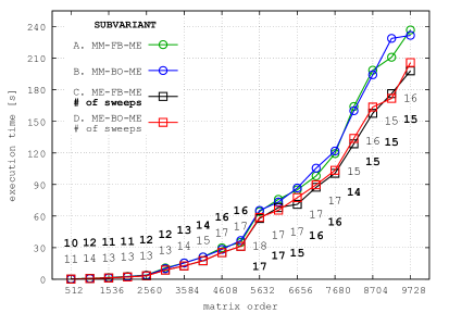
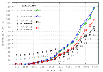
Table 21 in Appendix E contains the wall time for DHZ0-(me-fb-me), which is generally the fastest of the four subvariants.
In Table 2 the intervals of relative slowdown of other real single-GPU (me-fb-me) variants compared to DHZ0-(me-fb-me) (the reference variant) are given.
| ID | maximal relative | minimal relative | average relative |
| slowdown [%] | slowdown [%] | slowdown [%] | |
| 1 | 11.107853 | 0.984035 | 3.093490 |
| 2 | 17.137007 | 1.722547 | 4.870879 |
| 3 | 32.907217 | 3.144621 | 9.204879 |
| 4 | 0.328320 | -0.678588 | 0.139650 |
| 5 | 11.353652 | 1.395604 | 3.373963 |
| 6 | 17.962363 | 2.065662 | 5.199807 |
| 7 | 32.290521 | 3.511386 | 9.413653 |
5.2.2 Performance in the complex case
In the right subfigure of Figure 7 the wall execution time of four subvariants of ZHZ4 (the fastest of eight variants from Table 1 on the largest matrix pair) and the number of outer sweeps for two fastest subvariants on the small complex dataset are shown.
In Table 3 the intervals of relative slowdown of other complex single-GPU (me-fb-me) variants compared to ZHZ4-(me-fb-me) (the reference variant) are given. Since ZHZ0-(me-fb-me) is the fastest variant on average, differing from ZHZ4 only subtly (in the convergence criterion), ZHZ0 is used instead of ZHZ4 in the multi-GPU algorithm and in subsection 5.2.6. Table 22 in Appendix F shows the wall time for ZHZ0-(me-fb-me).
| ID | maximal relative | minimal relative | average relative |
|---|---|---|---|
| slowdown [%] | slowdown [%] | slowdown [%] | |
| 0 | 0.488301 | -6.403801 | -0.493666 |
| 1 | 2.309416 | -0.241201 | 0.841493 |
| 2 | 7.135216 | -1.206508 | 1.756809 |
| 3 | 12.632933 | 0.866139 | 3.167284 |
| 5 | 1.366689 | -0.442658 | 0.312471 |
| 6 | 8.423992 | 0.720393 | 2.287251 |
| 7 | 11.257148 | 1.092003 | 3.240513 |
5.2.3 Detailed timings of the main kernel’s subphases
Tables 4 and 5 show the percentages of time each subphase of the main kernel takes on a Volta GPU for the selected subvariants of the real and the complex single-GPU algorithm, respectively. As the problem size increases, the first and the fourth subphases (i.e., the matrix multiplications) start to dominate over the others. With a suitable modification for the recent GPU architectures like Ampere, the Hari–Zimmermann algorithm could therefore benefit from their dedicated hardware and instructions for speeding up the GEMM-like operations.
| subphases of [%] | subphases of [%] | |||||||
| 1 | 2 | 3 | 4 | 1 | 2 | 3 | 4 | |
| 512 | 12.3 | 10.0 | 53.8 | 23.9 | 20.9 | 17.0 | 21.3 | 40.7 |
| 1024 | 17.5 | 7.1 | 41.1 | 34.4 | 25.7 | 10.4 | 13.1 | 50.8 |
| 1536 | 20.6 | 5.3 | 34.1 | 40.0 | 28.2 | 7.3 | 9.3 | 55.2 |
| 2048 | 22.8 | 4.4 | 28.2 | 44.6 | 29.4 | 5.7 | 7.3 | 57.6 |
| 2560 | 24.9 | 3.7 | 23.3 | 48.0 | 30.6 | 4.6 | 5.9 | 59.0 |
| 3072 | 26.1 | 3.3 | 20.5 | 50.1 | 31.1 | 3.9 | 5.0 | 59.9 |
| 3584 | 26.5 | 2.9 | 18.7 | 51.8 | 31.2 | 3.4 | 4.4 | 61.0 |
| 4096 | 27.3 | 2.6 | 17.1 | 53.0 | 31.6 | 3.0 | 3.9 | 61.4 |
| 4608 | 27.8 | 2.4 | 15.4 | 54.4 | 31.7 | 2.7 | 3.5 | 62.1 |
| 5120 | 28.2 | 2.2 | 14.5 | 55.2 | 32.0 | 2.5 | 3.2 | 62.4 |
| 5632 | 28.8 | 2.0 | 13.2 | 56.0 | 32.2 | 2.2 | 2.9 | 62.7 |
| 6144 | 29.2 | 1.9 | 12.0 | 56.9 | 32.2 | 2.1 | 2.7 | 63.0 |
| 6656 | 29.4 | 1.8 | 11.7 | 57.2 | 32.4 | 1.9 | 2.5 | 63.2 |
| 7168 | 29.7 | 1.7 | 10.8 | 57.9 | 32.5 | 1.8 | 2.3 | 63.4 |
| 7680 | 30.0 | 1.7 | 10.1 | 58.3 | 32.5 | 1.8 | 2.1 | 63.6 |
| 8192 | 29.5 | 1.6 | 9.9 | 59.0 | 32.0 | 1.6 | 2.1 | 64.3 |
| 8704 | 30.3 | 1.5 | 8.9 | 59.2 | 32.6 | 1.7 | 1.9 | 63.8 |
| 9216 | 30.4 | 1.4 | 8.7 | 59.5 | 32.7 | 1.5 | 1.9 | 64.0 |
| 9728 | 30.6 | 1.4 | 8.2 | 59.9 | 32.7 | 1.5 | 1.7 | 64.1 |
| subphases of [%] | subphases of [%] | |||||||
| 1 | 2 | 3 | 4 | 1 | 2 | 3 | 4 | |
| 512 | 13.9 | 6.5 | 51.6 | 28.1 | 23.2 | 10.9 | 18.7 | 47.2 |
| 1024 | 19.6 | 4.7 | 35.8 | 39.9 | 27.2 | 6.5 | 10.8 | 55.5 |
| 1536 | 21.9 | 3.5 | 29.3 | 45.4 | 28.5 | 4.6 | 7.7 | 59.3 |
| 2048 | 24.7 | 2.8 | 23.3 | 49.2 | 30.2 | 3.5 | 6.0 | 60.3 |
| 2560 | 27.3 | 2.4 | 19.2 | 51.1 | 32.1 | 2.8 | 4.6 | 60.5 |
| 3072 | 28.4 | 2.1 | 16.3 | 53.2 | 32.5 | 2.4 | 3.9 | 61.2 |
| 3584 | 29.1 | 1.9 | 14.3 | 54.7 | 32.8 | 2.1 | 3.4 | 61.8 |
| 4096 | 29.5 | 1.7 | 12.9 | 55.9 | 32.9 | 1.8 | 3.0 | 62.3 |
| 4608 | 29.9 | 1.5 | 12.0 | 56.5 | 33.0 | 1.7 | 2.7 | 62.6 |
| 5120 | 30.1 | 1.4 | 11.2 | 57.3 | 33.1 | 1.5 | 2.4 | 63.0 |
| 5632 | 30.6 | 1.3 | 10.5 | 57.5 | 33.5 | 1.4 | 2.2 | 62.9 |
| 6144 | 30.8 | 1.2 | 9.7 | 58.3 | 33.4 | 1.3 | 2.1 | 63.2 |
| 6656 | 31.1 | 1.1 | 9.2 | 58.6 | 33.6 | 1.2 | 1.9 | 63.3 |
| 7168 | 31.3 | 1.1 | 8.5 | 59.2 | 33.6 | 1.1 | 1.8 | 63.5 |
| 7680 | 31.3 | 1.0 | 8.0 | 59.6 | 33.5 | 1.0 | 1.6 | 63.8 |
| 8192 | 32.2 | 1.0 | 7.4 | 59.4 | 34.2 | 1.0 | 1.6 | 63.3 |
| 8704 | 31.7 | 0.9 | 7.3 | 60.1 | 33.7 | 1.0 | 1.5 | 63.9 |
| 9216 | 31.7 | 0.9 | 7.1 | 60.3 | 33.7 | 0.9 | 1.4 | 64.0 |
| 9728 | 32.0 | 0.8 | 6.7 | 60.5 | 33.8 | 0.9 | 1.3 | 64.0 |
5.2.4 Intensities of the floating-point arithmetic operations
Tables 6 and 7 contain the relative intensity of floating-point operations with rounding across all invocations of all kernels (not only the main one, though other kernels’ contributions are negligible) on a Maxwell GPU. The columns names correspond to the double precision CUDA arithmetic intrinsics, while represents the calls to and functions (their constituent operations were not counted separately). The results strongly correlate with those from Tables 4 and 5; namely, the intensity of increases as the matrix multiplications take the larger portions of the overall time. For the smaller inputs the combined amount of divisions/reciprocals, square roots, and the function calls is in single percents, but according to (Arafa et al., 2019, Table IV) even such an amount has a considerable influence on the execution time; e.g., a division has on average close to 20 times the latency of a simple instruction (like ) on the Volta GPUs.
| 512 | 0.83 | 22.68 | 1.32 | 16.33 | 54.20 | 1.71 | 0.57 | 2.35 |
| 1024 | 0.55 | 15.86 | 0.91 | 11.18 | 68.29 | 1.17 | 0.39 | 1.64 |
| 1536 | 0.43 | 12.34 | 0.71 | 8.70 | 75.33 | 0.91 | 0.30 | 1.27 |
| 2048 | 0.34 | 9.99 | 0.57 | 7.01 | 80.06 | 0.74 | 0.25 | 1.03 |
| 2560 | 0.27 | 8.00 | 0.45 | 5.53 | 84.16 | 0.58 | 0.19 | 0.82 |
| 3072 | 0.23 | 6.86 | 0.38 | 4.72 | 86.44 | 0.49 | 0.16 | 0.71 |
| 3584 | 0.20 | 6.16 | 0.35 | 4.25 | 87.80 | 0.45 | 0.15 | 0.63 |
| 4096 | 0.17 | 5.43 | 0.31 | 3.71 | 89.31 | 0.39 | 0.13 | 0.56 |
| 4608 | 0.16 | 4.89 | 0.28 | 3.34 | 90.36 | 0.35 | 0.12 | 0.50 |
| 5120 | 0.14 | 4.51 | 0.26 | 3.09 | 91.10 | 0.33 | 0.11 | 0.46 |
| 5632 | 0.12 | 3.94 | 0.22 | 2.67 | 92.27 | 0.28 | 0.09 | 0.40 |
| 6144 | 0.11 | 3.62 | 0.20 | 2.45 | 92.89 | 0.26 | 0.09 | 0.37 |
| 6656 | 0.11 | 3.52 | 0.20 | 2.41 | 93.06 | 0.26 | 0.09 | 0.36 |
| 7168 | 0.10 | 3.13 | 0.18 | 2.13 | 93.85 | 0.22 | 0.07 | 0.32 |
| 7680 | 0.09 | 2.91 | 0.16 | 1.96 | 94.30 | 0.21 | 0.07 | 0.30 |
| 8192 | 0.09 | 2.85 | 0.16 | 1.94 | 94.39 | 0.21 | 0.07 | 0.29 |
| 8704 | 0.08 | 2.59 | 0.15 | 1.75 | 94.92 | 0.18 | 0.06 | 0.27 |
| 9216 | 0.08 | 2.48 | 0.14 | 1.68 | 95.13 | 0.18 | 0.06 | 0.25 |
| 9728 | 0.07 | 2.34 | 0.13 | 1.58 | 95.41 | 0.17 | 0.06 | 0.24 |
| 512 | 0.92 | 12.81 | 0.42 | 11.63 | 71.86 | 0.42 | 0.83 | 1.12 |
| 1024 | 0.53 | 7.46 | 0.24 | 6.63 | 83.78 | 0.24 | 0.47 | 0.65 |
| 1536 | 0.39 | 5.42 | 0.17 | 4.83 | 88.21 | 0.17 | 0.34 | 0.47 |
| 2048 | 0.30 | 4.16 | 0.13 | 3.68 | 90.98 | 0.13 | 0.26 | 0.36 |
| 2560 | 0.23 | 3.27 | 0.10 | 2.84 | 92.97 | 0.10 | 0.20 | 0.28 |
| 3072 | 0.19 | 2.70 | 0.08 | 2.33 | 94.21 | 0.08 | 0.16 | 0.23 |
| 3584 | 0.17 | 2.34 | 0.07 | 2.02 | 94.98 | 0.07 | 0.14 | 0.20 |
| 4096 | 0.15 | 2.03 | 0.06 | 1.74 | 95.66 | 0.06 | 0.12 | 0.17 |
| 4608 | 0.13 | 1.88 | 0.06 | 1.61 | 95.99 | 0.06 | 0.11 | 0.16 |
| 5120 | 0.12 | 1.71 | 0.05 | 1.46 | 96.35 | 0.05 | 0.10 | 0.15 |
| 5632 | 0.11 | 1.55 | 0.05 | 1.32 | 96.70 | 0.05 | 0.09 | 0.13 |
| 6144 | 0.10 | 1.40 | 0.04 | 1.19 | 97.02 | 0.04 | 0.08 | 0.12 |
| 6656 | 0.09 | 1.32 | 0.04 | 1.12 | 97.20 | 0.04 | 0.08 | 0.11 |
| 7168 | 0.09 | 1.20 | 0.04 | 1.03 | 97.44 | 0.04 | 0.07 | 0.10 |
| 7680 | 0.08 | 1.13 | 0.03 | 0.96 | 97.60 | 0.03 | 0.07 | 0.10 |
| 8192 | 0.07 | 1.03 | 0.03 | 0.88 | 97.81 | 0.03 | 0.06 | 0.09 |
| 8704 | 0.07 | 1.01 | 0.03 | 0.86 | 97.86 | 0.03 | 0.06 | 0.09 |
| 9216 | 0.07 | 0.96 | 0.03 | 0.81 | 97.96 | 0.03 | 0.06 | 0.08 |
| 9728 | 0.07 | 0.91 | 0.03 | 0.78 | 98.06 | 0.03 | 0.05 | 0.08 |
5.2.5 Accuracy in the real case
In the left subfigure of Figure 8 the normwise relative errors of four subvariants of DHZ0 are shown in a logarithmic scale, while in Table 8 the spectral condition numbers in the small real dataset are given, offering a justification for the non-monotonicity of the error graphs.
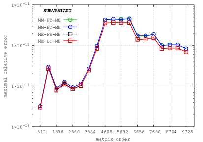
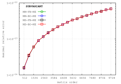
| 512 | 5632 | ||
| 1024 | 6144 | ||
| 1536 | 6656 | ||
| 2048 | 7168 | ||
| 2560 | 7680 | ||
| 3072 | 8192 | ||
| 3584 | 8704 | ||
| 4096 | 9216 | ||
| 4608 | 9728 | ||
| 5120 | – | – |
In Table 9 the spectral condition numbers in the small real dataset are given, without a corresponding error figure, which is almost indistinguishable from the left subfigure of Figure 8.
| 512 | 5632 | ||
| 1024 | 6144 | ||
| 1536 | 6656 | ||
| 2048 | 7168 | ||
| 2560 | 7680 | ||
| 3072 | 8192 | ||
| 3584 | 8704 | ||
| 4096 | 9216 | ||
| 4608 | 9728 | ||
| 5120 | – | – |
Figure 9 shows the numerical orthogonality of the left generalized singular vectors (left subfigure) and (right subfigure) across the small real dataset achieved by DHZ0.
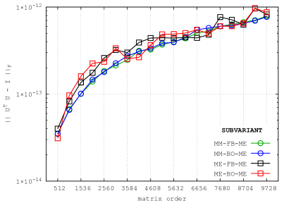
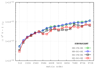
Tables 10 and 11 show the maximal relative errors in the generalized singular values computed by DHZ0-(me-fb-me) and DTGSJA from the Intel Math Kernel Library (version 2020.1.217 on an Intel Xeon Phi 7210 CPU), respectively, on the small real dataset.
| 512 | 5632 | ||
| 1024 | 6144 | ||
| 1536 | 6656 | ||
| 2048 | 7168 | ||
| 2560 | 7680 | ||
| 3072 | 8192 | ||
| 3584 | 8704 | ||
| 4096 | 9216 | ||
| 4608 | 9728 | ||
| 5120 | – | – |
| 512 | 5632 | ||
| 1024 | 6144 | ||
| 1536 | 6656 | ||
| 2048 | 7168 | ||
| 2560 | 7680 | ||
| 3072 | 8192 | ||
| 3584 | 8704 | ||
| 4096 | 9216 | ||
| 4608 | 9728 | ||
| 5120 | – | – |
The average relative errors in the computed generalized singular values in both the GPU and the CPU case are two to three orders of magnitude smaller than the maximal ones, as can be seen for the former in the supplementary material. By comparing Tables 10 and 11 it can be concluded that, in this sense and instance, the proposed GPU algorithm exhibits accuracy similar to the LAPACK’s DTGSJA.
5.2.6 Accuracy in the complex case
In the right subfigure of Figure 8 the normwise relative errors of four subvariants of ZHZ0 are shown in a logarithmic scale, while in Table 12 the spectral condition numbers in the small complex dataset are presented, offering a justification for a smooth shape of the error graphs.
| 512 | 5632 | ||
| 1024 | 6144 | ||
| 1536 | 6656 | ||
| 2048 | 7168 | ||
| 2560 | 7680 | ||
| 3072 | 8192 | ||
| 3584 | 8704 | ||
| 4096 | 9216 | ||
| 4608 | 9728 | ||
| 5120 | – | – |
In Table 13 the spectral condition numbers in the small complex dataset are given. A corresponding error figure would be almost identical to the right subfigure of Figure 8.
| 512 | 5632 | ||
| 1024 | 6144 | ||
| 1536 | 6656 | ||
| 2048 | 7168 | ||
| 2560 | 7680 | ||
| 3072 | 8192 | ||
| 3584 | 8704 | ||
| 4096 | 9216 | ||
| 4608 | 9728 | ||
| 5120 | – | – |
Figure 10 shows the numerical orthogonality of the left generalized singular vectors (left subfigure) and (right subfigure) on the small complex dataset achieved by ZHZ0.
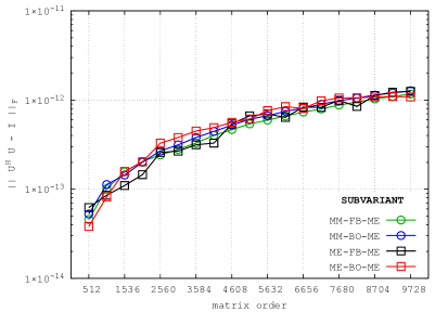
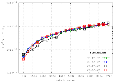
5.2.7 Conclusions
From Figure 7 it is obvious that mm gives a significantly slower execution than me at the outer level, and that fb is slightly faster than bo. From Tables 2 and 3 it is clear that the execution times across the variants do not widely differ, and that the enhanced dot-products from Appendix A add from a few percent to something more than to the wall time.
In both the real and the complex case the variant 0 with (me-fb-me) is a reasonable choice performance-wise.
Regarding the normwise relative errors on the matrices of moderate spectral conditions, as it is in the real case, the mm subvariants are almost indistinguishable, as are the me subvariants, with the latter being slightly more accurate than the former, as shown in the left subfigure of Figure 8. With the matrices of small spectral condition, as it is in the complex case, all subvariants are almost indistinguishable, as shown in the right subfigure of Figure 8. The spectral condition numbers were computed by Matlab R2019a.
In Table 14 the maximal relative normwise errors with respect to and in the real and the complex case on the small dataset for all variants of the single-GPU algorithm with (me-fb-me) are given.
| real case | complex case | |||
|---|---|---|---|---|
| ID | max. relative | max. relative | max. relative | max. relative |
| error w.r.t. | error w.r.t. | error w.r.t. | error w.r.t. | |
| 0 | ||||
| 1 | ||||
| 2 | ||||
| 3 | ||||
| 4 | ||||
| 5 | ||||
| 6 | ||||
| 7 | ||||
Looking at the minimal value in each data column, it is evident that, except for in the real case, the enhanced dot-products offer a small advantage in accuracy, but not so significant that it would not be offset by a drop in performance when the focus is on the latter.
Despite the low occupancy, Table 15 shows that all warps that can occupy a multiprocessor execute with almost full efficiency.
| nvprof metric | minimal | maximal |
|---|---|---|
| sm_52 architecture | value [%] | value [%] |
| achieved_occupancy | ||
| branch_efficiency | ||
| sm_efficiency | ||
| warp_execution_efficiency | ||
| warp_nonpred_execution_efficiency |
It is therefore expected that, should the present bottleneck on multiprocessors be removed in the future by increasing the register file (see subsection 3.5) as it has recently been done with the shared memory, the occupancy might increase as well, and with it the overall performance, while the efficiency would stay at the same high level.
5.3 Results with the multi-GPU algorithm
Due to a limited availability of GPUs in the testing environment, only the complex case in the variant 0 was tested on the large dataset and compared with a single-GPU baseline.
Here, the full accuracy testing was skipped, due to the huge computational demands of the matrix inversions and of the error calculation in extended precision. For , the relative errors in the corresponding outputs with one and with two GPUs (in both cases in all variants that were timed) were compared and all of them, for both and , were found to be less than . Also, for a given matrix, the relative errors in all cases differed less than , indicating that the multi-GPU algorithm did not introduce any instability in the computation.
5.3.1 A single-GPU baseline
In Table 16 the wall time in seconds and the number of the outermost sweeps are shown for the me-fb-me and the me-bo-me subvariants, with and without the column sorting, of the ZHZ0 single-GPU algorithm, as a baseline for the comparison with the multi-GPU algorithm. As the similar benefits of the column sorting were obvious in other trial tests runs, the non-sorting version was not considered for the full testing.
| me-fb-me | me-bo-me | column sort |
|---|---|---|
| 2063.19 s; 10 | 2248.48 s; 11 | yes |
| 3509.21 s; 17 | 3482.66 s; 17 | no |
5.3.2 The multi-GPU performance
In Tables 17, 18, 19, and 20 the wall time in seconds and the outermost sweep count are shown for the multi-GPU variants
respectively, run on two, four, and eight GPUs. The tests on two and four GPUs required a single node, and those on eight GPUs required two InfiniBand-connected nodes. When a particular test was not possible to be run due to an insufficient amount of the GPU RAM, “n/a” is shown in the test’s table cell.
| 2 GPUs | 4 GPUs | 8 GPUs | |
| 18432 | 3796.78 s; 5 | 2594.38 s; 6 | 1638.43 s; 7 |
| 24576 | 8869.04 s; 5 | 6718.15 s; 6 | 5134.84 s; 7 |
| 36864 | n/a | 21271.83 s; 6 | 12560.23 s; 7 |
| 2 GPUs | 4 GPUs | 8 GPUs | |
|---|---|---|---|
| 18432 | 1606.17 s; 9 | 1085.34 s; 9 | 774.97 s; 9 |
| 24576 | 3536.52 s; 9 | 2568.67 s; 9 | 2004.23 s; 9 |
| 36864 | n/a | 7643.07 s; 9 | 4870.56 s; 9 |
| 2 GPUs | 4 GPUs | 8 GPUs | |
|---|---|---|---|
| 18432 | 4295.87 s; 5 | 2903.28 s; 6 | 1806.63 s; 7 |
| 24576 | 10098.11 s; 5 | 7693.07 s; 6 | 5825.82 s; 7 |
| 36864 | n/a | 23611.93 s; 6 | 14225.79 s; 7 |
| 2 GPUs | 4 GPUs | 8 GPUs | |
|---|---|---|---|
| 18432 | 1759.48 s; 10 | 1201.17 s; 10 | 849.58 s; 10 |
| 24576 | 3926.69 s; 10 | 2863.27 s; 10 | 2224.73 s; 10 |
| 36864 | n/a | 9248.23 s; 11 | 5877.18 s; 11 |
5.3.3 Conclusions
It is clear from Tables 17, 18, 19, and 20, that the multi-GPU variant is to be recommended when performance matters.
Dividing the shortest single-GPU baseline wall time from Table 16 for with the wall times from Table 18 for the same but with a different number of GPUs, it can be derived that the speedup with two GPUs is , with four GPUs is , and with eight GPUs is . These speedups could be even lower on a slower network or if there were fewer than four GPUs present per node.
It would be interesting to see for what number of GPUs, depending on the input sizes, the speedup peaks and starts falling, but that is beyond reach of the testing environment. In the absence of such information, a safe rule of thumb would be to use a modest number of GPUs on a fast interconnect for a given problem, such that they are fully utilized in the terms of multiprocessors and memory.
6 Conclusions and future work
The proposed algorithms compute the generalized SVD efficiently, accurately, and almost entirely on the GPU(s). The single-GPU algorithm requires a CPU only for the controlling purposes. The multi-GPU algorithm involves a substantial amount of unavoidable communication, but scales acceptably as long as each GPU if kept fully utilized.
Several generalizations of the algorithms’ design are possible for the other implicit Jacobi-type methods that are to be ported to the GPUs. One such method is a computation of the generalized hyperbolic SVD (GHSVD) Bojanczyk (2003) by a modification of the implicit Hari–Zimmermann algorithm, as described in Singer et al. (2020). {acks} This research was performed using the resources of computer cluster Isabella based in SRCE - University of Zagreb University Computing Centre.
We would like to thank the associate editor and the anonymous referees for their recommendations for improving this manuscript. {dci} The Authors declare that there is no conflict of interest. {funding} This work has been supported in part by Croatian Science Foundation under the project IP–2014–09–3670. {sm} The full testing results and some details of the chosen Jacobi strategies are provided as the supplementary material sm.pdf.
The source code is available in https://github.com/venovako/GPUHZGSVD repository. For comparing with the accuracy results a tag https://github.com/venovako/GPUHZGSVD/tree/rev0 should be used. Note that the actual names of the kernels, variables, etc. in the code are different. The names in the paper are chosen for the simplicity of referencing.
References
- Alter et al. (2003) Alter O, Brown PO and Botstein D (2003) Generalized singular value decomposition for comparative analysis of genome-scale expression data sets of two different organisms. P. Natl. Acad. Sci. USA 100(6): 3351–3356. 10.1073/pnas.0530258100.
- Anderson et al. (1999) Anderson E, Bai Z, Bischof C, Blackford S, Demmel J, Dongarra J, Du Croz J, Greenbaum A, Hammarling S, McKenney A and Sorensen D (1999) LAPACK Users’ Guide. edition. Philadelphia, PA, USA: Society for Industrial and Applied Mathematics. ISBN 0-89871-447-8 (paperback).
- Arafa et al. (2019) Arafa Y, Badawy AA, Chennupati G, Santhi N and Eidenbenz S (2019) Low overhead instruction latency characterization for NVIDIA GPGPUs. In: 2019 IEEE High Performance Extreme Computing Conference (HPEC). pp. 1–8. 10.1109/HPEC.2019.8916466.
- Bai (1994) Bai Z (1994) A parallel algorithm for computing the generalized singular value decomposition. J. Parallel Distrib. Comput. 20(3): 280–288. 10.1006/jpdc.1994.1027.
- Bojanczyk (2003) Bojanczyk AW (2003) An implicit Jacobi-like method for computing generalized hyperbolic SVD. Linear Algebra Appl. 358(1): 293–307. 10.1016/S0024-3795(02)00394-4.
- Boukaram et al. (2018) Boukaram WH, Turkiyyah G, Ltaief H and Keyes DE (2018) Batched QR and SVD algorithms on GPUs with applications in hierarchical matrix compression. Parallel Comput. 74: 19–33. 10.1016/j.parco.2017.09.001.
- Cannon (1969) Cannon LE (1969) A Cellular Computer to Implement the Kalman Filter Algorithm. PhD Thesis, Montana State University, Bozeman, MT, USA.
- Cempel (2009) Cempel C (2009) Generalized singular value decomposition in multidimensional condition monitoring of machines–A proposal of comparative diagnostics. Mech. Syst. Signal Pr. 23(3): 701–711. 10.1016/j.ymssp.2008.07.004.
- Drmač (1997) Drmač Z (1997) Implementation of Jacobi rotations for accurate singular value computation in floating point arithmetic. SIAM J. Sci. Comput. 18(4): 1200–1222. 10.1137/S1064827594265095.
- Graillat et al. (2015) Graillat S, Lauter C, Tang PTP, Yamanaka N and Oishi S (2015) Efficient calculations of faithfully rounded -norms of -vectors. ACM Trans. Math. Software 41(4): art. no. 24. 10.1145/2699469.
- Hammond et al. (2014) Hammond JR, Schäfer A and Latham R (2014) To INT_MAX… and beyond! Exploring large-count support in MPI. In: 2014 Workshop on Exascale MPI at Supercomputing Conference. pp. 1–8. 10.1109/ExaMPI.2014.5.
- Hari (1984) Hari V (1984) On Cyclic Jacobi Methods for the Positive Definite Generalized Eigenvalue Problem. PhD Thesis, FernUniversität–Gesamthochschule, Hagen, Germany.
- Hari (2018) Hari V (2018) Globally convergent Jacobi methods for positive definite matrix pairs. Numer. Algorithms 79(1): 221–249. 10.1007/s11075-017-0435-5.
- Hari (2019) Hari V (2019) On the global convergence of the complex HZ method. SIAM J. Matrix Anal. Appl. 40(4): 1291–1310. 10.1137/19M1265594.
- Hari et al. (2010) Hari V, Singer S and Singer S (2010) Block-oriented -Jacobi methods for Hermitian matrices. Linear Algebra Appl. 433(8–10): 1491–1512. 10.1016/j.laa.2010.06.032.
- Hari et al. (2014) Hari V, Singer S and Singer S (2014) Full block -Jacobi method for Hermitian matrices. Linear Algebra Appl. 444: 1–27. 10.1016/j.laa.2013.11.028.
- Howland et al. (2003) Howland P, Jeon M and Park H (2003) Structure preserving dimension reduction for clustered text data based on the generalized singular value decomposition. SIAM J. Matrix Anal. Appl. 25(1): 165–179. 10.1137/S0895479801393666.
- Howland et al. (2006) Howland P, Wang J and Park H (2006) Solving the small sample size problem in face recognition using generalized discriminant analysis. Pattern Recogn. 39(2): 277–287. 10.1016/j.patcog.2005.06.013.
- Luk (1985) Luk FT (1985) A parallel method for computing the generalized singular value decomposition. J. Parallel Distrib. Comput. 2(3): 250–260. 10.1016/0743-7315(85)90027-9.
- Mantharam and Eberlein (1993) Mantharam M and Eberlein PJ (1993) Block recursive algorithm to generate Jacobi–sets. Parallel Comput. 19: 481–496. 10.1016/0167-8191(93)90001-2.
- Mary et al. (2015) Mary T, Yamazaki I, Kurzak J, Luszczek P, Tomov S and Dongarra J (2015) Performance of random sampling for computing low-rank approximations of a dense matrix on GPUs. In: Proceedings of the International Conference for High Performance Computing, Networking, Storage and Analysis (SC ’15). pp. 1–11 (art. no. 60). 10.1145/2807591.2807613.
- Message Passing Interface Forum (2015) Message Passing Interface Forum (2015) MPI: A Message-Passing Interface Standard, Version 3.1. High Performance Computing Center Stuttgart (HLRS).
- Novaković (2015) Novaković V (2015) A hierarchically blocked Jacobi SVD algorithm for single and multiple graphics processing units. SIAM J. Sci. Comput. 37(1): C1–C30. 10.1137/140952429.
- Novaković (2017) Novaković V (2017) Parallel Jacobi-type algorithms for the singular and the generalized singular value decomposition. PhD Thesis, University of Zagreb, Croatia. URL https://urn.nsk.hr/urn:nbn:hr:217:515320.
- Novaković and Singer (2011) Novaković V and Singer S (2011) A GPU-based hyperbolic SVD algorithm. BIT 51(4): 1009–1030. 10.1007/s10543-011-0333-5.
- Novaković et al. (2015) Novaković V, Singer S and Singer S (2015) Blocking and parallelization of the Hari–Zimmermann variant of the Falk–Langemeyer algorithm for the generalized SVD. Parallel Comput. 49: 136–152. 10.1016/j.parco.2015.06.004.
- NVIDIA Corp. (2019) NVIDIA Corp (2019) CUDA C Programming Guide v10.1.243. URL https://docs.nvidia.com/cuda/archive/10.1/cuda-c-programming-guide/.
- Paige and Saunders (1981) Paige CC and Saunders MA (1981) Towards a generalized singular value decomposition. SIAM J. Numer. Anal. 18(3): 398–405. 10.1137/0718026.
- Quintana-Ortí et al. (1998) Quintana-Ortí G, Sun X and Bischof C (1998) A BLAS-3 version of the QR factorization with column pivoting. SIAM J. Sci. Comp. 19(5): 1486–1494. 10.1137/S1064827595296732.
- Senaratne and Tellambura (2013) Senaratne D and Tellambura C (2013) GSVD beamforming for two-user MIMO downlink channel. IEEE T. Veh. Technol. 62(6): 2596–2606. 10.1109/TVT.2013.2241091.
- Singer et al. (2020) Singer S, Di Napoli E, Novaković V and Čaklović G (2020) The LAPW method with eigendecomposition based on the Hari–Zimmermann generalized hyperbolic SVD. SIAM J. Sci. Comput. 42(5): C265–C293. 10.1137/19M1277813.
- Singer et al. (2012) Singer S, Singer S, Novaković V, Ušćumlić A and Dunjko V (2012) Novel modifications of parallel Jacobi algorithms. Numer. Algorithms 59: 1–27. 10.1007/s11075-011-9473-6.
- Slapničar (1998) Slapničar I (1998) Componentwise analysis of direct factorization of real symmetric and Hermitian matrices. Linear Algebra Appl. 272: 227–275. 10.1016/S0024-3795(97)00334-0.
- Tomov et al. (2010) Tomov S, Dongarra J and Baboulin M (2010) Towards dense linear algebra for hybrid GPU accelerated manycore systems. Parallel Comput. 36(5–6): 232–240. 10.1016/j.parco.2009.12.005.
- Van Loan (1976) Van Loan CF (1976) Generalizing the singular value decomposition. SIAM J. Numer. Anal. 13(1): 76–83. 10.1137/0713009.
- Zhao et al. (2010) Zhao Q, Rutkowski TM, Zhang L and Cichocki A (2010) Generalized optimal spatial filtering using a kernel approach with application to EEG classification. Cogn. Neurodyn. 4(4): 355–358. 10.1007/s11571-010-9125-x.
- Zhou and van der Veen (2017) Zhou M and van der Veen AJ (2017) Blind separation of partially overlapping data packets. Digit. Signal Process. 68: 154–166. 10.1016/j.dsp.2017.06.009.
- Zimmermann (1969) Zimmermann K (1969) Zur Konvergenz eines Jacobiverfahren für gewönliche und verallgemeinerte Eigenwertprobleme. Dissertation no. 4305, Eidgenössische Technische Hochschule, Zürich, Switzerland.
Appendix A Enhanced dot-product computation
In CUDA, the rounding mode can be specified explicitly for each arithmetic operation using the intrinsic functions. That makes an ideal setting for employing a trick from Graillat et al. (2015) to cheaply compute possibly more accurate real and complex dot-products.
For two real vectors and of the same length, their enhanced dot-product would require one FMA and one negation per a pair of vector elements, in addition to one multiplication. Also, adding the partial sums together needs two sum-reductions instead of one, as follows.
Let and be the elements of and at the same, arbitrary index, and let __dmul_rd stand for a CUDA intrinsic performing a multiplication with rounding towards . Take
Then, by looking separately at the both possible signs of , it can be shown that for the rounding error of the multiplication extracted by the FMA holds . By sum-reducing , no cancellation can occur. That value may be added to the sum-reduction result on , to form the final dot-product.
For two complex vectors and of the same length, defining an enhanced dot-product is not so unambiguous. A special case of computing can be handled as follows. For an element of , take
considering the real part of , and
considering the imaginary part of . Let , , , and be the sum-reductions of all , , , and , respectively. Then, return , where the quantities are the four -sums above, ordered increasingly.
However, such an approach requires four reductions. To simplify it by trading off accuracy for speed, let be the sum of the rounding errors. Then, if , take , else let , and return the sum-reduction of as an approximation of .
The real dot-product and the simpler of the two procedures for computing of the square of the Euclidean norm of a complex vector have been incorporated in the special variants of the algorithm and tested, both without a huge slowdown but also without a significant effect on accuracy of the result, as explained in section 5.
Appendix B A single-GPU out-of-core algorithm
Algorithm 7 gives an overview of a single-GPU “out-of-core” algorithm, when the whole data does not fit into the GPU RAM, but at least one block pair of , , and does.
This algorithm has not been implemented, but essentially the bstep1(s/n) kernel would be converted to a kernel OoCstep1(s/n) that operates on a suitably sized subset of all block pivots of an outer step. The subset is loaded into the GPU RAM beforehand, and is brought back, transformed, to the CPU. That process is repeated until all block pivots in the outer step have been transformed, exactly as they would be by a single call to bstep1(s/n). Apart from being inefficient, such an approach cannot handle the case when not even a single block pair can fit into a GPU. For the GPU RAM being and the matrices complex and square, would then have to be larger than 11 million, in which case the multi-GPU algorithm is a must anyway.
Appendix C Warp-shuffle -reduction of 32 doubles
In Figure 11 a warp-shuffle sum-reduction of 32 double-precision values is shown, where each thread in a warp holds one value at the start, and all threads get the sum at the end. The loop over i is manually unrolled in the code.
__device__ __forceinline__
double dSum32(const double x) {
  int lo0, hi0, lo1, hi1;
  double x0 = x, x1;
  for (int i = 16; i; i >>= 1) {
    lo0 = __double2loint(x0);
    hi0 = __double2hiint(x0);
    lo1 = __shfl_xor_sync(~0u, lo0, i);
    hi1 = __shfl_xor_sync(~0u, hi0, i);
    x1 = __hiloint2double(hi1, lo1);
    x0 = __dadd_rn(x0, x1);
  }
  lo0 = __double2loint(x0);
  hi0 = __double2hiint(x0);
  lo1 = __shfl_sync(~0u, lo0, 0);
  hi1 = __shfl_sync(~0u, hi0, 0);
  return __hiloint2double(hi1, lo1);
}
Appendix D An implementation of the main kernel’s subphases 1 and 4 with the batched matrix multiplication from cuBLAS
The subphases 1 and 4 of the main kernel (see subsection 3.5) could have also been decoupled and implemented separately, by the batched matrix multiplication routines from the cuBLAS library. For that, more than twice the GPU RAM is required, to maintain two copies of the data. The first copy, called “actual”, holds the current state of the computation at the start of each block step. The second one, called “shadow”, is used as a temporary buffer, in which the new state is assembled at the end of the step. These copies then change the roles by a simple swap of the pointers to them. Schematically, this layout can be represented as
Let be the field in which the computations take place. For the complex algorithm, a data layout with the real and the imaginary components kept separately is no longer viable because cuBLAS does not support it.
Furthermore, let be the number of block column pairs processed at each block step, i.e., the number of thread blocks launched. An additional workspace of square matrices of order is required, where , as
In this GPU RAM workspace the transformation matrices accumulated in the subphase 3 will be stored from the shared memory of each thread block.
For each there is an associated pair of block indices drawn from the chosen block strategy for the current block step, with the subscripts omitted when they are implied by the context. Then, the block columns of the actual copy can be logically grouped and denoted as
and a similar notation is used for the shadow copy as well.
Replacing the subphase 1 involves forming the lower block-triangle of the Grammian matrices and as
by two batched GEMM calls: one for , and another for .
Each batched GEMM call forms all , , and blocks, since the inputs are all of the same dimensions, as well as the outputs. Forming the remaining, upper-right blocks is not necessary, since the subphase 2 reads only the lower triangle as the Grammian matrices are Hermitian. The diagonal blocks should be formed by the batched SYRK or HERK operations instead, but at present they are not implemented in cuBLAS. Each is stored in the first rows of the shadow copy , starting from its th column, and similarly for and , from where they are loaded by the modified subphase 2 into the shared memory and their Cholesky factorizations are then computed as before. Note that this approach involves storing and in the GPU RAM, only to be read afterwards into the shared memory, what is a redundant memory traffic avoided by the original implementation.
The modified main kernel, after completing the subphase 2, computes the transformation matrices in the subphase 3, and stores them from the shared memory to the workspace (another redundant memory traffic). For the postmultiplications, i.e., the block column updates, consider each to be logically partitioned as
Now, compute a partial update of by a single batched GEMM call (and similarly for and ), where for each ,
and complete the update by another batched GEMM call as
A swap of the pointers to the copies, , completes the block step. See the var subdirectory of the code repository for a double precision implementation.
A benefit of this alternative is that it significantly reduces the register pressure in the main kernel, e.g., close to halving the required number of registers on a Volta GPU. However, that is offset by allocating more than twice the GPU RAM, which is still a scarce resource, and consequently by reducing the maximal input sizes per GPU. Also, setting up a huge number of pointers for each batched GEMM call, as well as the redundant stores to and loads from the GPU RAM of the contents of the shared memory makes the prototype implementation about 20 times slower on average than the original one. Therefore, this version of the algorithm is not recommendable on the present hardware.
Appendix E The QR factorizations as an alternative to the main kernel’s subphases 1 and 2 for the ill-conditioned input matrices
As mentioned in subsection 2.3, for a highly ill-conditioned input matrix the formation of the Grammians of its block-column pairs by the main kernel’s subphase 1 might result in several numerically singular or indefinite blocks, on which the Cholesky factorizations in the subphase 2 are bound to fail. In such cases the affected (or, for simplicity, all) block-column pairs have to be shortened by the QR factorizations instead. Ideally, the factorizations would employ column pivoting (see, e.g., Quintana-Ortí et al. (1998) and the LAPACK’s XGEQP3 routines, ), but it can be inefficient on GPUs Mary et al. (2015).
The batched non-pivoted QR factorization routine from cuBLAS could be used with the memory layout proposed for Appendix D, where the vectors would be stored in the buffer. Replacing the subphases 1 and 2 that way would require to pack the block columns, e.g., and , consecutively in the copy for each (similarly for ). The packed block-column pairs in the copy would then be subject to the QR factorizations, and the upper triangular factors would be extracted from it by the modified subphase 3. The postmultiplication subphase would remain as in Appendix D. However, this approach would also suffer from the redundant traffic between the shared and the global memory.
Another approach is to keep the original memory layout and have two “streaming” QR factorizations (one for the assigned block-column pair of , and another for the same-indexed block-column pair of ) embedded into the main kernel. Each factorization reads from the global memory only once, in chunks, never writes to it (since the matrix does not have to be applied again or restored), and leaves the upper triangular factor in the shared memory where the subphase 3 expects it to be. The full details of this in-kernel QR factorization can be found in (Novaković, 2015, subsection 4.2) for double precision, while a complex version would be implemented similarly.
Table 21 demonstrates that close to eightfold slowdown can be expected on a Volta GPU with the in-kernel QR factorizations on larger matrices, even when using the simplest, unsafe Frobenius norm computations inside them.
| [s] | [s] | [s] | [s] | ||||
|---|---|---|---|---|---|---|---|
| 512 | 0.83 | 0.20 | 4.1 | 5632 | 437.48 | 57.81 | 7.6 |
| 1024 | 3.57 | 0.69 | 5.1 | 6144 | 522.05 | 68.10 | 7.7 |
| 1536 | 7.30 | 1.24 | 5.9 | 6656 | 544.53 | 71.13 | 7.7 |
| 2048 | 12.87 | 2.02 | 6.4 | 7168 | 674.35 | 87.38 | 7.7 |
| 2560 | 21.86 | 3.31 | 6.6 | 7680 | 775.09 | 100.64 | 7.7 |
| 3072 | 61.46 | 8.69 | 7.1 | 8192 | 1015.82 | 128.65 | 7.9 |
| 3584 | 90.87 | 12.66 | 7.2 | 8704 | 1233.91 | 157.62 | 7.8 |
| 4096 | 128.73 | 17.52 | 7.3 | 9216 | 1389.86 | 176.37 | 7.9 |
| 4608 | 186.27 | 25.22 | 7.4 | 9728 | 1551.47 | 198.03 | 7.8 |
| 5120 | 230.32 | 31.26 | 7.4 | – | – | – | – |
Appendix F Performance-wise comparison of a CPU and a single-GPU implementation of the complex Hari–Zimmermann GSVD
Table 22 shows the speedup of the complex single-GPU algorithm on the small dataset versus the CPU GHSVD algorithm from Singer et al. (2020), with the signature matrix for the latter being . The GHSVD’s implementation was not tuned for the simpler GSVD computation. If it were, it could have been at least twice as fast on a more modern CPU, but nevertheless noticeably slower than the GPU algorithm on the Volta architecture.
| [s] | [s] | [s] | [s] | ||||
|---|---|---|---|---|---|---|---|
| 512 | 1.22 | 0.26 | 4.7 | 5632 | 422.37 | 65.27 | 6.5 |
| 1024 | 9.52 | 0.81 | 11.8 | 6144 | 671.15 | 77.85 | 8.6 |
| 1536 | 21.52 | 1.68 | 12.8 | 6656 | 659.89 | 92.55 | 7.1 |
| 2048 | 45.40 | 2.98 | 15.3 | 7168 | 756.02 | 109.74 | 6.9 |
| 2560 | 70.81 | 5.46 | 13.0 | 7680 | 971.17 | 131.07 | 7.4 |
| 3072 | 114.68 | 13.30 | 8.6 | 8192 | 1931.45 | 182.53 | 10.6 |
| 3584 | 164.41 | 17.96 | 9.2 | 8704 | 1258.28 | 208.32 | 6.0 |
| 4096 | 397.57 | 23.63 | 16.8 | 9216 | 1520.19 | 236.45 | 6.4 |
| 4608 | 270.74 | 30.77 | 8.8 | 9728 | 1646.25 | 269.04 | 6.1 |
| 5120 | 360.70 | 40.11 | 9.0 | – | – | – | – |
Appendix G Computational pitfalls of the GEVD of versus the GSVD of
This small example shows what happens with the GEVD of versus the GSVD of when one of the matrices (here, ) is even mildly ill-conditioned. All results were obtained by Matlab R2020a Update 3.
Let and , with , be given as
Clearly, and are non-singular, so and are symmetric positive definite. If, e.g., (rounded to double precision) is taken, the generalized eigenvalues of , also rounded to double precision, are
where and are the Grammians of the rational (symbolic) representations of and , respectively, while is a sorted representation of the symbolic output of .
When computing in double precision, two routes can be taken. The first one finds the generalized singular values of and , i.e., ,
and squares them to get the generalized eigenvalues ,
which are close to , i.e., the exact ones.
The second route computes from and by a “proper” GEVD routine, getting
with the lower three generalized eigenvalues vanishing.
The spectral condition numbers of the matrices are:
i.e., the condition numbers of and are the squares of those of and , respectively, which is easily shown by taking the SVD of or and expressing or in terms of it. Therefore, a mildly ill-conditioned matrix causes its Grammian to be severely ill-conditioned and the GEVD fails, so the matrix multiplications have to be avoided in such a case by computing the GSVD of instead.
Motivated by the previous example, 16 pairs of square real matrices of order were generated in quadruple precision by the adapted symmetric indefinite factorization with complete pivoting Slapničar (1998), and then rounded to double precision, such that , with , was fixed, while varied, with the prescribed values for , for . The matrices and were generated from the given positive eigenvalues by the LAPACK’s testing routine DLAROR adapted to quadruple precision, ensuring that their condition numbers are as close to the prescribed ones as possible, and that their ensuing factorizations were identical in effect to the Cholesky factorizations with diagonal pivoting. Then, the generalized singular values of , i.e., the singular values of , were computed in high precision with 32 significant as
by Matlab R2020b, to be compared against in two ways.
The generalized singular values of were recomputed by the DHZ0-(me-fb-me) variant, and the generalized eigenvalues of were obtained by the cusolverDnDsygvd routine from the cuSOLVER library, to assess how well they approximate squares of the generalized singular values. The maximal relative errors in the generalized singular values computed by the last two approaches were then found, with , as
where , , and were sorted descendingly. Here, denotes a conversion to the Intel’s extended 80-bit datatype.
As it can be seen in Table 23, the generalized singular values computed by taking square roots of the generalized eigenvalues rapidly lose accuracy when the condition of increases beyond about , where is the machine precision. Entirely invalid results are possible, indicated by , since the smallest six generalized eigenvalues of were computed as negative and the square roots could not have been taken. The generalized singular values computed by a “proper” GSVD (the HZ algorithm) remained relatively accurate in all cases, though.
However, if it is known in advance that a particular GSVD problem on is extremely well conditioned, solving it as the GEVD of might be significantly faster. From , , and , it follows that finding (the generalized eigenvalues) and (the generalized eigenvectors) suffices to compute , , and . Normalizing the columns of both and (with the extracted norms on its diagonal) are obtained, and similarly for and , but and might not be as orthogonal as those that come from a “proper” GSVD. For the left generalized singular vectors to be computed, the original matrices and have to be preserved, which, along with a non-trivial amount of workspace needed for the GEVD routine call, more than doubles the memory requirements compared to those of the single-GPU Hari–Zimmermann GSVD algorithm.
The matrices and are formed on a GPU, each by a single call of the cuBLAS’ routine cublasDsyrk (or cublasZherk in the complex case) from and , respectively. Then, the cuSOLVER’s (legacy) routine cusolverDnDsygvd (or cusolverDnZhegvd in the complex case) solves the GEVD problem on . For and multiplications the cuBLAS’ cublasDgemm (or cublasZgemm in the complex case) routine can be used. Finally, the normalizing, as described above, can be performed by a custom kernel similar to rescale.
The computation as described above, but skipping the normalization, was compared performance-wise to the DHZ0-(me-fb-me) and the ZHZ0-(me-fb-me) variants. Let D stand for the ratio of the wall times of the “proper” GSVD and the GSVD-using-GEVD approaches in the real, and Z in the complex case, on the respective small datasets. Then, D and Z, as shown in Table 24, are relaxed upper bounds on the expected speedup by the GEVD approach (the actual speedup should be somewhat smaller) on the GPUs. For comparison, about – speedup is expected on the modern CPUs in the complex case Singer et al. (2020) on a set of small-to-medium sized matrices. But it should never be understated that there are hard limits to the applicability of the GEVD approach to the GSVD when the condition of the problem is high or unknown in advance.
| D [] | Z [] | D [] | Z [] | ||
|---|---|---|---|---|---|
| 512 | 6.57 | 8.28 | 5632 | 49.92 | 26.63 |
| 1024 | 9.39 | 10.49 | 6144 | 49.25 | 25.30 |
| 1536 | 10.76 | 11.75 | 6656 | 41.63 | 24.02 |
| 2048 | 11.92 | 12.53 | 7168 | 42.38 | 23.60 |
| 2560 | 13.88 | 15.05 | 7680 | 41.82 | 23.45 |
| 3072 | 26.32 | 24.72 | 8192 | 45.45 | 26.95 |
| 3584 | 27.76 | 22.83 | 8704 | 46.42 | 25.92 |
| 4096 | 30.06 | 21.93 | 9216 | 44.71 | 25.07 |
| 4608 | 34.12 | 21.35 | 9728 | 43.41 | 24.50 |
| 5120 | 34.15 | 21.53 | – | – | – |
Vedran Novaković received his Ph.D. in Mathematics in
2017 from University of Zagreb, Croatia, where he started his career
as a teaching assistant. He also worked at STFC Daresbury
Laboratory, UK, as a computational scientist and at Universidad
Jaime I, Spain. He is interested in parallel algorithms of
numerical linear algebra, especially eigenvalue and singular value
algorithms.
![]() https://orcid.org/0000-0003-2964-9674
https://orcid.org/0000-0003-2964-9674
Sanja Singer is a tenured professor of Mathematics at the
Faculty of Mechanical Engineering and Naval Architecture, University
of Zagreb, Croatia. She received her Ph.D. in Mathematics in 1997
from the same University. Her interests lie in accurate and
high-performance algorithms of numerical linear algebra, especially
matrix factorization algorithms, eigenvalue and singular value
algorithms.
![]() https://orcid.org/0000-0002-4358-1840
https://orcid.org/0000-0002-4358-1840