Significance of Gravitational Nonlinearities on the Dynamics of Disk Galaxies

Abstract

The discrepancy between the visible mass in galaxies or galaxy clusters, and that inferred from their dynamics is well known. The prevailing solution to this problem is dark matter. Here we show that a different approach, one that conforms to both the current Standard Model of Particle Physics and General Relativity, explains the recently observed tight correlation between the galactic baryonic mass and the measured accelerations in the galaxy. Using direct calculations based on General Relativity’s Lagrangian, and parameter-free galactic models, we show that the non-linear effects of General Relativity make baryonic matter alone sufficient to explain this observation. Our approach also shows that a specific acceleration scale dynamically emerges. It agrees well with the value of the MOND acceleration scale.

1 Introduction

An empirical tight relation between accelerations calculated from the galactic baryonic content and the observed accelerations in galaxies has been reported by McGaugh et al. (McGaugh et al., 2016, hereafter MLS2016); larger accelerations are accounted for by the baryonic matter, i.e. there is no missing mass problem, while in lower acceleration regions, dark matter or gravitation/dynamical laws beyond Newton’s are necessary. This correlation is surprising because galactic dynamics should be dictated by the total mass (believed to be predominantly dark), but instead the baryonic mass information alone is sufficient to get the observed acceleration. A tight connection between dark and baryonic matter distributions would explain the observation, but such connection has not been expected. While the relation from MLS2016—including its small scatter—can be reproduced with dark matter models, (Ludlow et al., 2017), the consistency of the measured correlation width with the observational uncertainties suggests a dynamical origin rather than an outcome of galaxy formation, since this would add an extra component to the width.

Dynamical studies of galaxies typically use Newton’s gravity. However, it has been argued that once galactic masses are considered, relativistic effects arising from large masses (rather than large velocities) may become important (Deur, 2009, 2017, 2019). Their physical origin is that in General Relativity (GR), gravity fields self-interact. In this article, we explore whether these effects can explain the relation in MLS2016 without requiring dark matter or modifying gravitation as we currently know it.

The article is organized as follows. We first outline the self-interaction effects in GR, then discuss in Section 3 the empirical tight dependence of observed acceleration on baryonic mass in disk (i.e. lenticular and spiral) galaxies. In Section 4, we use GR’s equations to compute the correlation. These CPU-intensive calculations allow us to study only a few galaxies, modeled as bulge-less disks. To cover the full range of disk galaxy morphologies, including those with significant bulge, in Section 5 we develop two dynamical models of disk galaxies in different but complementary ways: uniform sampling (Section 5.1) and random sampling (Section 5.2) of the galactic parameter space. In Section 6 we show the results from these models, and compare them to observations. Finally, in Section 7, we summarize our findings and their importance.

2 Self-Interaction Effects in General Relativity

Field self-interaction makes GR non-linear. The phenomenon is neglected when Newton’s law of gravity is used, as is typically done in dynamical studies of galaxies or galaxy clusters. However, such a phenomenon becomes significant once the masses involved are large enough. Furthermore, it is not suppressed by low velocity—unlike some of the more familiar relativistic effects—as revealed by e. g. the inspection of the post-Newtonian equations (Einstein et al., 1938). In fact, the same phenomenon exists for the strong nuclear interaction and is especially prominent for slow-moving quark systems (heavy hadrons), in which case it produces the well-known quark confining linear potential.

The connection between self-interaction and non-linearities is seen e.g. by using the polynomial form of the Einstein-Hilbert Lagrangian (see e.g. Salam, 1974; Zee, 2013)

$$\mathcal{L}=\frac{\sqrt{\mathrm{det}(g_{\mu\nu})}\,g_{\mu\nu}R^{\mu\nu}}{16\pi G}=\sum_{n=0}^{\infty}\left(16\pi GM\right)^{n/2}\left[\varphi^{n}\big{(}\partial\varphi\partial\varphi-(16\pi GM)^{1/2}\varphi T\big{)}\right]$$ (1)

where $g_{\mu\nu}$ is the metric, $R_{\mu\nu}$ the Ricci tensor, $T_{\mu\nu}$ the energy-momentum tensor, $M$ the system mass and $G$ is the gravitational constant. In the natural units ($\hbar=c=1$) used throughout this article, $[G]=\mbox{energy}^{-2}$. The polynomial is obtained by expanding $g_{\mu\nu}$ around a constant metric $\eta_{\mu\nu}$ of choice, with $\varphi_{\mu\nu}\equiv g_{\mu\nu}-\eta_{\mu\nu}$ the gravitational field. The brackets are shorthands for sums over Lorentz-invariant terms (Deur, 2017). For example, the $n=0$ term is explicitly given by the Fierz-Pauli Lagrangian (Fierz & Pauli, 1939):

$$\left[\partial\varphi\partial\varphi-\sqrt{16\pi GM}\varphi T\right]=\frac{1}{2}\partial^{\lambda}\varphi_{\mu\nu}\partial_{\lambda}\varphi^{\mu\nu}-\frac{1}{2}\partial^{\lambda}\varphi_{\mu}^{\mu}\partial_{\lambda}\varphi_{\nu}^{\nu}-\partial^{\lambda}\varphi_{\lambda\nu}\partial_{\mu}\varphi^{\mu\nu}+\partial^{\nu}\varphi_{\lambda}^{\lambda}\partial^{\mu}\varphi_{\mu\nu}-\sqrt{(16\pi GM)}\varphi^{\mu\nu}T_{\mu\nu}.$$

While Eq. (1) is often used to study quantum gravity—with questions raised regarding its applicability in that context, see e.g. (Padmanabhan, 2008)—we stress that the calculations and results presented here are classical, and thus not subject to the difficulties arising from quantum gravity nor the issues raised in (Padmanabhan, 2008). Field self-interaction originates from the $n>0$ terms in Eq. (1), distinguishing GR from Newton’s theory, for which the Lagrangian is given by the $n=0$ term. One consequence of the $n>0$ terms is that they effectively increase gravity’s strength. It is thus reasonable to investigate whether they may help to solve the missing mass problem. In fact, it was shown that they allow us to quantitatively reproduce the rotation curves of galaxies without need for dark matter, also providing a natural explanation for the flatness of the rotation curves (Deur, 2009).

The phenomenon underlying these studies is ubiquitous in Quantum Chromodynamics (QCD, the gauge theory of the strong interaction). The GR and QCD Lagrangians are similar in that they both contain field self-interaction terms. In fact, they are topologically identical (see Appendix A where the similarities and differences between GR and QCD are discussed). In QCD, the effects of field self-interaction is well-known as they are magnified by the large QCD coupling, typically $\alpha_{s}\simeq 0.1$ at the transition between perturbative and strong regimes (Deur et al., 2016).

In GR, self-interaction effects become important when $GM$—which in the natural unit used in this manuscript has a length dimension—reaches a fraction of the characteristic length $L$ of the system. Numerical lattice calculations show that $GM\approx 10^{-3}L$ characterizes systems where self-interaction cannot be neglected (Deur, 2017)). At the particle level, gravity, and a fortiori its non-linearities, are automatically ignored since $GM_{p}\approx 10^{-39}r_{p}$ ($M_{p}$ and $r_{p}$ are the proton mass and radius, respectively), and hence $GM_{p}/r_{p}/\alpha_{s}\approx 10^{-40}$. However the ratio becomes $10^{-2}$ for galactic systems, making it reasonable to ask whether QCD-like GR’s self-interaction effects should be considered. That value characterizes e.g. typical disk galaxies, galaxies interacting in a cluster, and the Hulse-Taylor binary. A large mass discrepancy is apparent when the dynamics of galaxies and galaxy clusters are analyzed, while the Hulse-Taylor binary is already known to be governed by strong gravity.

In QCD, a critical effect of self-interaction is a stronger binding of quarks, resulting in their confinement. In GR, self-interaction likewise increases gravity’s binding, which can provide an origin for the missing mass problem. However, one may question the relevance of field self-interaction at large galactic radii $r$. At these distances the missing mass problem is substantial, while the small matter density should make the self-interaction effects negligible. The answer is in the behavior of the gravitational field lines; once they are distorted at small $r$ due to the larger matter density, they evidently remain so even if the matter density becomes negligible (no more field self-interaction, i.e. no further distortion of the field lines), preserving a form of potential different to that of Newton. Thus, even if the gravity field becomes weak, the deviation from Newton’s gravity remains.

A key feature for this article is the suppression of self-interaction effects in isotropic and homogeneous systems (Deur, 2009):

$\bullet$ In a two-point system, large $\sqrt{GM}$ or $\alpha_{s}$ values lead to a constant force between the two points (and a vanishing force elsewhere), i.e. the string-like flux-tube that is well-known in QCD.

$\bullet$ Due to the symmetry of a homogeneous disk, the flux collapses only outside of the disk plane, thereby confining the force to two dimensions. Consequently, the force between the disk center and a point in the disk at a distance $r$ decreases as $1/r$.

$\bullet$ For a homogeneous sphere, the force recovers its usual $1/r^{2}$ behavior since the flux has no particular direction or plane of collapse.

This symmetry dependence has led to the discovery of a correlation between the missing mass of elliptical galaxies and their ellipticity (Deur, 2014). This also illustrates the point of the previous paragraph: even if the matter density in the disk decreases quickly with $r$, the missing mass problem—which in our approach comes from the difference between the GR and Newtonian treatments—grows worse since the difference between the $1/r$ GR force in the 2D disk and the $1/r^{2}$ Newtonian force grows with $r$. This offers a simple explanation for the relation reported in MLS2016: although densities, and thus accelerations, are largest at small $r$, the $1/r-1/r^{2}$ difference between the GR and Newtonian treatments remains moderate. However, the difference becomes important at large $r$, where accelerations are small. Furthermore, at small $r$, the $1/r^{2}$ force is recovered for GR due to finite disk thickness $h_{z}$, since isotropy is restored for $r\lesssim h_{z}$. This recovery is amplified since disk galaxies often contain a central high-density bulge that is usually nearly spherical (Méndez-Abreu et al., 2008). The departure from the $1/r^{2}$ behavior then occurs after the bulge-disk transition.

3 Baryonic Mass—Acceleration Dependence

The correlation between the radial acceleration traced by rotation curves ($g_{\rm{\scriptscriptstyle obs}}$) and that predicted by the known distribution of baryons ($g_{\rm{\scriptscriptstyle bar}}$) reported in MLS2016 was established after analyzing 2693 points in 153 disk galaxies with varying morphologies, masses, sizes, and gas fractions. The MLS2016 authors found a good functional form fitting the correlation:

$$g_{\rm{\scriptscriptstyle obs}}={{g_{\rm{\scriptscriptstyle bar}}}\over{1-e^{-\sqrt{g_{\rm{\scriptscriptstyle bar}}/g_{\dagger}}}}},$$ (2)

where $g_{\dagger}$ is an acceleration scale, the only free parameter of the fit. In the remainder of the article, we show that the observed correlation may be entirely due to the non-linear GR effects which are neglected in the traditional Newtonian analysis. In the next section, we use a direct GR calculation of rotation curves for actual galaxies modeled as bulge-less disks (Deur, 2009). We show that when the galactic bulge of the actual galaxy is negligible, the calculation yields a relation that agrees with the empirical correlation from MLS2016. In the two subsequent sections, we develop models to include the effect of bulges and to account for the variation of morphology of disk galaxies.

4 Direct Calculations

The rotation curves of several disk galaxies were computed in (Deur, 2009) based on Eq. (1) and using numerical lattice calculations in the static limit (Deur, 2017). The method is summarized in Appendix B. The two-body lattice calculations described there show that given the magnitude of galactic masses, the self-interaction traps the field. For a two-body system, i.e. a system characterized by one dominant dimension, field trapping results in a constant force since a force magnitude at a given distance $r$ is proportional to the field line density crossing an elementary surface. Thus, for one-dimensional systems, the force is constant and the potential grows linearly with the distance $r$, as obtained in the numerical lattice calculations (Deur, 2017, 2009). We can extend this result to a two-dimensional system such as a disk. For a field restricted to two dimensions, the flux disperses over an angle rather than a solid angle, which yields a force that varies as $1/r$, i.e. obeys a logarithmic potential. Extending the one-dimensional result to the two-dimensional disk case of galaxies assumes that the spread of the mass within the disk area does not compromise the trapping of the field in two dimensions. This is reasonable since most galactic baryonic mass is concentrated near its center. This reasoning and the hypothesis that the field remains trapped for a disk are supported by a different approach that uses a mean-field method applied to a thin disk distribution (Deur, 2020). The mean field calculation yields a large-distance logarithmic potential when the mass of the disk is sufficient (see Fig. 7 in Appendix B).

The calculations of Ref. (Deur, 2009) neglect the galactic bulge and approximate a spiral galaxy with a disk featuring an exponentially-falling density profile. They were carried out for nearly bulge-less Hubble types 5 and 6 galaxies (NGC 2403, 3198 and 6503), and for Hubble types 3 and 4 galaxies (NGC 2841, 2903 and 7331), which have moderate bulges. Using these results, we can compute the total acceleration $g_{{\rm{\scriptscriptstyle SI}}}$ stemming from baryonic matter and including GR’s field self-interaction—analog of $g_{{\rm{\scriptscriptstyle obs}}}$ from MLS2016. Plotting it versus the Newtonian acceleration $g_{{\rm{\scriptscriptstyle N}}}$ obtained from the same distribution of baryonic matter, but ignoring GR’s self-interaction—analog of $g_{{\rm{\scriptscriptstyle bar}}}$ from MLS2016—one obtains the results shown in the top panel of Fig. 1.

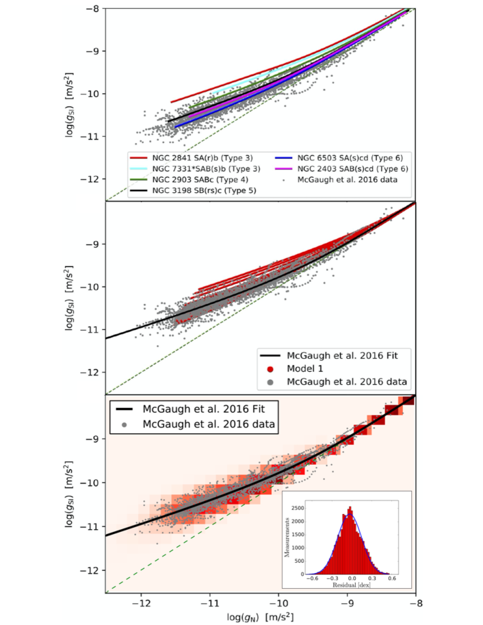
Figure 1: Correlation between the acceleration accounting for GR’s self-interaction, $g_{\rm{\scriptscriptstyle SI}}$, and the acceleration computed with Newtonian gravity, $g_{\rm{\scriptscriptstyle N}}$, plotted along with the correlation observed in MLS2016 (grey circles). Top: Lagrangian-based calculations for various Hubble type galaxies. The galaxies are approximated as pure (bulge-less) disks. The calculations agree well with observation when this approximation is justified (types 5 and 6 galaxies) but depart gradually from observation as the bulge becomes more important. Middle: Model 1 with uniform sampling of the galactic parameter phase space. Bottom: Model 2 with galactic parameter phase space sampled following observed distributions (1146 galaxies, sampled at 100 radial values are shown). The density of the data points obtained with Model 2 is encoded by the color scale. The dashed line indicates $g_{\rm{\scriptscriptstyle SI}}=g_{\rm{\scriptscriptstyle N}}$. Embedded in the bottom panel is the residual distribution between the result of Model 2 and the best fit to the observational data (black line) beyond the transition radius, $r>r_{t}$ (for points within the transition radius, $r\leq r_{t}$, the deviation from the MLS2016 fit is, by construction, small but systematic; hence the residual has no statistical meaning in that region).

The curves for types 5 and 6 galaxies agree well with the observed correlation, thereby providing an explanation for it in bulge-less galaxies. However, the curves for types 3 and 4 galaxies, while qualitatively following the correlation, overestimate $g_{{\rm{\scriptscriptstyle SI}}}$ and lie on the edge of the observed distribution. That the empirical correlation is reproduced only for bulge-less galaxies supports that 1) the correlation from MLS2016 is explainable by GR’s self-interaction without requiring dark matter or modification of the known laws of nature, and 2) at large acceleration, i.e. typically for small galactic radii, the bulge reduces the value of $g_{{\rm{\scriptscriptstyle SI}}}$ since self-interaction effects cancel for isotropically distributed matter.

Although based directly on the GR’s Lagrangian, the lattice approach is limited since it is computationally costly and applies only to simple geometry, limiting the study to only a few late Hubble type galaxies at one time. To study the correlation from MLS2016 over the wide range of disk galaxy morphologies, we developed two models based on: 1) the $1/r$ gravitational force resulting from solving Eq. (1) for a disk of axisymmetrically distributed matter; and 2) the expectation that GR field self-interaction effects cancel for spherically symmetric distributions, such as that of a bulge, restoring the familiar $1/r^{2}$ force.

5 Dynamical Models

To circumvent the limitations of the direct lattice calculation, we constructed two elementary models for disk galaxies. They both compute the acceleration including GR’s self-interaction, $g_{\rm{\scriptscriptstyle SI}}$, and the Newtonian acceleration due to the baryonic matter, $g_{\rm{\scriptscriptstyle N}}$. Both $g_{{\rm{\scriptscriptstyle SI}}}$ and $g_{\rm{\scriptscriptstyle N}}$ are computed at a set of radii $r$, from the galactic center to its outermost parts. This is carried out for galaxies with their characteristics sampling the observed correlations reported in literature.

The modeled galaxies have two components: a spherical bulge and a larger disk. Both contain only baryonic matter following the light distribution, i.e. there is no dark matter and gas is either neglected or follow the stellar distribution.

The bulge is modeled with the projected surface brightness Sérsic profile (Sérsic, 1963) used in (Méndez-Abreu et al., 2008): $I_{b}(R)=I_{e}10^{-b_{n}[(R/R_{e})^{1/n}-1]}$, where $R$ is the projected radius, $I_{e}$ is the surface brightness at the half-light radius $R_{e}$, $n$ is the Sérsic parameter and $b_{n}\approx 0.868n-0.142$ (Caon et al., 1993). The internal mass density $\rho_{b}(r)$, where $r$ is the deprojected radius, is computed from the surface brightness by numerically solving the Abel integral. Since GR’s self-interaction effects cancel for isotropic homogeneous distributions, the potential in the bulge has the usual Newtonian form, $\Phi_{b}(r)=GM_{b}^{\rm enc}(r)/r$, where $M_{b}^{\rm enc}(r)$ is the bulge mass enclosed within a sphere of radius $r$.

The disk is modeled with the usual surface brightness radial profile $I_{d}(R)=I_{0}e^{-R/h}$, where $I_{0}$ is the central surface brightness, $h$ is the disk scale length, and possible effects from the disk thickness are neglected. Again, the corresponding mass density $\rho_{d}(r)$ is computed from the Abel integral. Self-interaction in a homogeneous disk leads to a potential $\Phi_{d}(r)=G^{\prime}M_{d}^{\rm enc}(r)\ln(r)$, with $M_{d}^{\rm enc}(r)$ the disk mass enclosed within a radius $r$, and $G^{\prime}$ the effective coupling of gravity in two dimensions, which depends on the physical characteristics of the disk (Deur, 2017); see detailed discussion in Appendix C.

The quantities characterizing a galaxy—the bulge and disk masses, $M_{b}$, $M_{d}$ (from which $\rho_{b,0}$ and $\rho_{d,0}$ are obtained, respectively), $R_{e}$, $n$ and $h$—span their observed ranges for S0 to Sd galaxies (Méndez-Abreu et al., 2008; Graham & Worley, 2008; Sofue, 2015). There are known relations between these quantities (Méndez-Abreu et al., 2008; Sofue, 2015):

$$\log(R_{e})=0.91(7)\log(h)-0.40(3),$$ (3)

$$\log(n)=0.18(5)R_{e}+0.38(2),$$ (4)

$$\log(M_{d})=0.58(32)\log(M_{b})+0.002(79).$$ (5)

We use values of $R_{e}$ and $M_{b}$ from the ranges of observed values to obtain the remaining galactic characteristics—$h$, $n$, $M_{d}$—through Eqs. (3)-(5). Thus, there are no adjustable parameters in our models.

We stress that the accuracy of the empirical relations Eqs. (3)-(5) is not critical to this work, their purpose being only to provide reasonable values of the galactic parameter space we select. While the simplicity of our models would make it of limited interest for investigating the intricate peculiarities of galaxies, such simplicity is beneficial for the present study: no numerous parameters nor phenomena (e.g. baryonic feedback) are needed for adjustment to reproduce the correlation from MLS2016. That the correlation emerges directly from basic models underlines the fundamental nature of the correlation.

The two dynamical models introduced in the remainder of this section share the above description. From here, they differ in two aspects. The first is in how the observed correlations in Eqs. (3)-(5) are implemented: Model 1 enforces the correlations strictly, while Model 2 allows for the parameter space to be randomly sampled. The second difference is in representing the transition radius, $r_{t}$, between the bulge-dominated regime near the center and disk-dominated regime : Model 1 explicitly sets the transition at twice the typical bulge scale, $r_{t}=2R_{e}$, while Model 2 defines $r_{t}$ as the radius at which the forces due to the two components—the bulge and the disk—are equal.

5.1 Model 1: Uniform Sampling of the Galactic Parameter Space

This model generates a galaxy set representative of disk galaxy morphologies by uniformly sampling the values of the galactic characteristics discussed in the previous section. The model strictly enforces Eqs. (3)-(5). This offers the advantage of simplicity, e.g. clarity, speed and robustness. Actual correlations, however, vary in their strengths. Hence, strictly implementing a correlation between quantities $a$ and $b$, and another between $a$ and $c$, would result in quantities $b$ and $c$ being also correlated, while if the actual correlations between $a$ and $b$, and $a$ and $c$ are both weak, then $b$ and $c$ may not be correlated. For example, propagating correlations among different galactic characteristics yields an inadequate relation between $M_{b}$ and $M_{d}$: $M_{d}\propto M_{b}^{-\alpha\pm\Delta}$, with $\Delta\gg\alpha=31$. To circumvent this problem, we use $h\propto R_{e}^{1.0}$, $M_{b}\propto R_{e}^{0.1}$, $n\propto R_{e}^{0.1}$ and $M_{d}\propto h^{1.0}$, in rough agreement with the correlations from Refs. (Méndez-Abreu et al., 2008; Khosroshahi et al., 2000).

The correlations are applied strictly, i.e. without accounting for the scatter seen in actual data, since systematically spanning the observed typical ranges for the quantities contributes to the width of the correlation reported in MLS2016, and accounting for such scatter would partly double-count, and thus overestimate, the width.

Inside the spherical bulge-dominated region (denoted by subscript $r<r_{t}$), the self-interaction cancels, and the GR and Newtonian accelerations are the same:

$$g_{{\rm{\scriptscriptstyle SI}},r<r_{t}}(r)=g_{{\rm{\scriptscriptstyle N}},r<r_{t}}(r)={{G}\over{r^{2}}}\left(M^{\rm enc}_{b}(r)+M^{\rm enc}_{d}(r)\right),$$ (6)

where

$$M^{\rm enc}_{b}(r) =4\pi\int_{0}^{r}{\tilde{r}}^{2}\rho_{b}({\tilde{r}})d{\tilde{r}},$$ (7)

$$M^{\rm enc}_{d}(r) =2\pi\int_{0}^{r}{\tilde{r}}\rho_{d}({\tilde{r}})d{\tilde{r}}.$$ (8)

In the disk-dominated region (denoted by subscript $r>r_{t}$), numerical lattice calculations indicate that self-interaction leads to a collapse in the gravitational field lines (Deur, 2009, 2017). The bulge density there is less significant than that of the disk, but is still present. The total acceleration is:

$$g_{{\rm{\scriptscriptstyle SI}},r>r_{t}}(r)={{G}\over{r^{2}}}M^{\rm enc}_{b}(r)+{{G}\over{r}}^{\prime}M^{\rm enc}_{d}(r).$$ (9)

The Newtonian acceleration $g_{{\rm{\scriptscriptstyle N}},r>r_{t}}$ in this region retains the form given in Eq. (6).

$G^{\prime}$ is determined by requiring the accelerations to match at $r_{t}$: $g_{{\rm{\scriptscriptstyle SI}},r<r_{t}}(r_{t})=g_{{\rm{\scriptscriptstyle SI}},r>r_{t}}(r_{t})$. Thus, $G^{\prime}=G/r_{t}$, by construction. The justification for this choice of $G^{\prime}$ is explained in detail in Appendix C.

The accelerations in the bulge and disk regions are smoothly connected using a Fermi-Dirac function centered at $r_{t}=2R_{e}$ and of width $r_{t}/2$: $D(r)=1/\big{(}1+e^{2(r-r_{t})/r_{t}}\big{)}$. Therefore, the acceleration with self-interaction is:

$$g_{{\rm{\scriptscriptstyle SI}}}(r)=D(r)g_{{\rm{\scriptscriptstyle SI}},r<r_{t}}(r)+\Big{(}1-D(r)\Big{)}g_{{\rm{\scriptscriptstyle SI}},r>r_{t}}(r),$$ (10)

while the Newtonian acceleration is:

$$g_{{\rm{\scriptscriptstyle N}}}(r)={{G}\over{r^{2}}}\left(M^{\rm enc}_{b}(r)+M^{\rm enc}_{d}(r)\right).$$ (11)

The choice of width value for $D(r)$ influences little the result: abruptly transitioning between bulge and disk, i.e. using a step-function rather than $D(r)$, yields quantitatively similar results. The small dependence on the functional form for the transition is also supported by the agreement between Models 1 and 2 which use different methods for the transition, as we discuss next.

5.2 Model 2: Random Sampling of the Galactic Parameter Space

For Model 2, we randomly generate the galaxy characteristics with gaussian distributions centered at the observed parameter values, and of widths determined by the observed distributions. In order to sample a realistic galaxy parameter space, we apply two types of cuts on the generated galaxy characteristics. The first type of cut ensures that the randomly sampled galaxy characteristics simultaneously satisfy Eqs. (3)-(5). A candidate galaxy is generated by first randomly sampling distributions of $R_{e}$ and $M_{b}$ separately, and then using them to randomly sample the observed correlations in Eqs. (3)-(5) to obtain $h$, $n$ and $M_{d}$. These are then combined to find $\rho_{b,0}$ and $\rho_{d,0}$, thereby completing the parameter set for a single candidate galaxy. This particular candidate galaxy then passes the first cut if its characteristics satisfy all of the correlations to within one standard deviation. Galaxies which pass this first cut are shown as orange and red circles in Fig. 2. The second type of cut is outlined below.

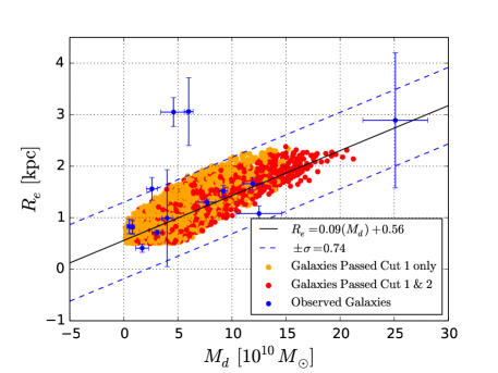
Figure 2: $R_{e}$ vs. $M_{d}$. Observed values are shown as blue circles (Sofue, 2015). The best $\chi^{2}$ fit to the observed data is denoted with a solid line, and one dex in dashed lines. Orange circles denote generated galaxies which passed the first cut only, while the red circles denote those who passed both cuts. The galaxies represented by the red circles are disk galaxies, while those corresponding to the orange circles are too bulge-dominated to qualify as such.

The transition between the bulge-dominated and the disk-dominated regions is implemented with a step-function $H(x)=1$ for $x<0$, and 0 otherwise, such that at $r_{t}$, the acceleration is kept continuous by the proper choice of $G^{\prime}$. The transition radius $r_{t}$ is defined as the radial location at which the acceleration due to the disk alone is equal to that due to the bulge alone:

$$G{M_{b}^{\rm enc}(r_{t})\over{r_{t}^{2}}}=G^{\prime}{M_{d}^{\rm enc}(r_{t})\over{r_{t}}},$$ (12)

with $G^{\prime}=G/r_{t}$ (see Appendix C). This choice of $G^{\prime}$ simplifies the condition for the transition $r_{t}$ to

$$M_{b}^{\rm enc}(r_{t})=M_{d}^{\rm enc}(r_{t}).$$ (13)

Some bulge-dominated galaxies will not have such a transition within $r=100$ kpc, and are removed from the sample. This is the second type of cut applied on the parameter space. Galaxies that pass both the first and the second types of cuts are shown as red circles in Fig. 2. Essentially, orange circles denote galaxies that are largely bulge-dominated and thus cannot qualify as disk galaxies. The red circles represent those galaxies having small to moderates bulges which qualify them as disk galaxies.

Models 1 and 2 use different methods for the bulge-disk transition. The agreement between the two models suggests that they are indifferent to a particular method. The acceleration including self-interaction is

$$g_{{\rm{\scriptscriptstyle SI}}}(r)=H(r-r_{t})g_{{\rm{\scriptscriptstyle SI}},r<r_{t}}(r)+\Big{(}1-H(r-r_{t})\Big{)}g_{{\rm{\scriptscriptstyle SI}},r>r_{t}}(r),$$ (14)

where $g_{{\rm{\scriptscriptstyle SI}},r<r_{t}}(r)$ and $g_{{\rm{\scriptscriptstyle SI}},r>r_{t}}(r)$ are given in Eqs. (6)-(9) and $g_{{\rm{\scriptscriptstyle N}}}(r)$ in Eq. (11).

In Model 2, we also modeled the effect of the bulge being spheroidal rather than spherical by introducing a polar dependence: $\rho_{b}(r,\phi)=\rho_{b}(r)(1-\epsilon\cos^{2}\phi)$, with $\rho_{b}(r)$ the spherical bulge density used in Models 1 and 2. This refinement did not noticeably change the results, thereby further proving their robustness.

6 Results

6.1 Comparison with observations

Direct lattice calculation and the two dynamical models allow us to compute the accelerations for a set of galaxies whose characteristics follow the typical observed ranges for disk galaxies. The acceleration including non-linear self-interaction ($g_{{\rm{\scriptscriptstyle SI}}}$) is plotted in Fig. 1 versus the acceleration computed with the same baryonic mass distribution but assuming Newtonian gravity ($g_{{\rm{\scriptscriptstyle N}}}$). This is compared to the observed correlation between $g_{{\rm{\scriptscriptstyle obs}}}$ and $g_{{\rm{\scriptscriptstyle bar}}}$ reported in MLS2016. The top panel shows the results for the direct calculation, the middle panel the results for Model 1, and bottom panel for Model 2. Since Model 2 samples the full parameter space selected by the cuts, but with statistical weights favoring the more probable parameter space loci, the results must be plotted as data point densities, the higher densities being indicated by the darker colors. Our computed correlations agree well with the empirical observation, without invoking dark matter or new laws of gravity/dynamics. To quantitatively assess this agreement, we averaged $g_{{\rm{\scriptscriptstyle SI}}}$ over all galaxies and also performed a fit of our simulated data using the same form used in MLS2016, i.e. Eq. (2). The best fit and the average $\langle\log(g_{{\rm{\scriptscriptstyle SI}}})\rangle$ versus $\log(g_{{\rm{\scriptscriptstyle N}}})$ are shown in Fig. 3. Our fit parameter $g^{\rm Mod2}_{\dagger}=9.71\pm 0.27\times 10^{-11}~{}{\rm m/s^{2}}$ is compatible with that of MLS2016, $g_{\dagger}=1.20\pm 0.02\mbox{(stat)}\pm 0.24\mbox{(syst)}\times 10^{-10}~{}{\rm m/s^{2}}$. This consistency is also manifests in the nearly overlapping residuals displayed in the insert of Fig. 3. This demonstrates quantitatively the agreement between our model and the data reported in MLS2016. We must remark that, despite this good agreement, $g^{\rm Mod2}_{\dagger}$ was not optimized to fit those of MLS2016, but that it results directly from Model 2 as described in Section 5.2. In fact, it cannot be adjusted since our models have no free parameters.

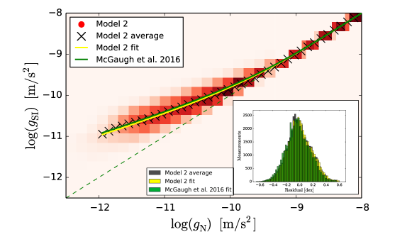
Figure 3: The acceleration accounting for GR’s self-interaction, $g_{{\rm{\scriptscriptstyle SI}}}$, versus that computed with Newtonian gravity, $g_{{\rm{\scriptscriptstyle N}}}$. The yellow line shows the best fit to our data simulated with Model 2 (red color density plot) using the form in Eq. (2). The black x’s are the average $\langle\log(g_{{\rm{\scriptscriptstyle SI}}})\rangle$. The yellow line and x’s can be compared to the MLS2016 fit, shown by the green line. The insert displays the residual between our simulated data and the MLS2016 fit (green histogram, already shown in Fig. 1), the residual using our fit (yellow histogram) and the one using $\langle g_{{\rm{\scriptscriptstyle SI}}}\rangle$ (black histogram).

6.2 Emerging characteristic acceleration scale

The transition scale between the two regimes in Model 2 is defined such as the location where forces from the bulge and disk are equal; see Eq. (12). The acceleration at the transition is shown in Fig. 4, in which the distribution peaks at $a(r_{t})=1.25\pm 0.06\times 10^{-10}$ ms^-2. The sharp peaking indicates that its mode can define a characteristic transition acceleration. In our Model 2, this one is consistent with the acceleration parameter $a_{0}\approx 1.2\times 10^{-10}$ ms^-2 in the MOND theory (Milgrom, 1983). Thus, $a_{0}$ can be explained as the acceleration at the radius where the self-interaction effects become important, that is, in the context of our present model, where the disk mass overtakes the bulge mass and causes a transition from the $1/r^{2}$ 3D force to the $1/r$ 2D force. For bulgeless disk galaxies, $r_{t}$ emerges dynamically, see discussion in Appendix C, and a direct calculation is necessary to obtain it.

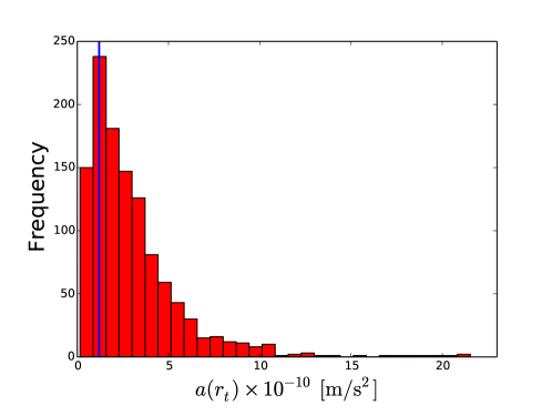
Figure 4: Acceleration at the transition radius $r_{t}$ for the set of galaxies generated in Model 2. The vertical line denotes $a_{0}=1.2\times 10^{-10}~{}{\rm m/s^{2}}$ from MOND.

6.3 Systematic studies of the residual width

One important finding of MLS2016 is that the width of their observed correlation is compatible with the uncertainty on the data. This poses a problem for a natural dark matter explanation since the baryonic matter-dark matter feedback mechanisms that would be necessary to correlate baryonic and dark matter distributions would partly depend on the history of the galaxy formation, as shown in MLS2016. In the present approach, because of the dependence of $r_{t}$ on the geometry and mass distributions, it may seem at first that the $g_{{\rm{\scriptscriptstyle N}}}$ vs $g_{{\rm{\scriptscriptstyle SI}}}$ correlation should depend on the specifics of a particular galaxy, increasing the width of the correlation. The criterium for determining $r_{t}$ in Model 2 is the equality of the disk and bulge forces, and therefore of the accelerations. The bulge and disk mass distributions and characteristic lengths being correlated, the acceleration at $r_{t}$ tends to cluster around a single value (see Fig. 4). Because the $g_{{\rm{\scriptscriptstyle N}}}$ vs $g_{{\rm{\scriptscriptstyle SI}}}$ correlation is not sensitive to small variations of where the acceleration transition happens on the $g_{{\rm{\scriptscriptstyle N}}}=g_{{\rm{\scriptscriptstyle SI}}}$ dashed line of Fig. 1, any dependence on galaxy specificities is suppressed. In fact, a change of $a_{0}$ by the variance extracted from Fig. 4 does not appreciably affect Fig. 1. We can quantitatively verify this by investigating whether large correlations exist between the galaxy characteristics and the residual shown in Fig. 1. Large correlations would disagree with the MLS2016 finding that their relation has no intrinsic width, and with the further verification in Ref. (Lelli et al., 2017) that the MLS2016 residual does not correlate with galaxy properties. We used the Pearson correlation coefficient $c_{p}$ to check for linear correlations between the residual and each galaxy properties—$R_{e}$, $h$, $M_{b}$ and $M_{d}$. Since the possible correlations could be non-linear, we also used the Spearman $c_{s}$ and the Kendall $c_{k}$ rank correlation coefficients. To maximize the sensitivity, we investigated the correlations at a fixed acceleration value, selected to be $-11.1\leq\log(g_{{\rm{\scriptscriptstyle N}}})\leq-11$, viz we checked whether galaxy characteristics are correlated with $g_{{\rm{\scriptscriptstyle SI}}}$, along the vertical line at $\log(g_{{\rm{\scriptscriptstyle N}}})\approx-11$ for the simulated data shown on the bottom panel of Fig. 1. The value $\log(g_{{\rm{\scriptscriptstyle N}}})\approx-11$ is optimal because there, the width is large, which maximizes the sensitivity to possible correlations, while the statistics remain important. Selecting $\log(g_{{\rm{\scriptscriptstyle N}}})\approx-11$ and computing correlation coefficients reveals that small correlations are present between the residual and the galaxy characteristics, see Fig. 5 for an example with $R_{e}$. (The other galaxy characteristics $h$ and $M_{b}$ also display correlations, albeit smaller. $M_{d}$ is not correlated.) To quantitatively investigate the effect of these correlations on the $g_{{\rm{\scriptscriptstyle N}}}$ vs $g_{{\rm{\scriptscriptstyle N}}}$ relation, we first take note that they are largely linear. This is suggested by the value of $c_{p}$ being similar to $c_{s}$ and $c_{k}$, as well as by the fact that polynomial fits of the residual vs galaxy characteristic distribution are numerically close to a linear fit. The approximate linearity of the correlations is confirmed by fitting linearly the correlations, then removing the linear dependence using the fit result. While $c_{p}$ calculated for the modified distributions must be zeroed by construction, the new $c_{s}$ and $c_{k}$ would reveal no remaining correlation only if the initial correlations had been linear. We indeed find negligible values of all the correlation coefficients for the modified distributions, e.g. $c_{p}=-6\times 10^{-17}$, $c_{s}=-4\times 10^{-3}$ ($p-$value $0.85$) and $c_{k}=-2\times 10^{-3}$ ($p-$value $0.87$) for $R_{e}$. By simultaneously applying this procedure for the distributions of the residual versus $R_{e}$, $h$, $M_{d}$ or $M_{b}$, we obtain a rms of 0.1812 for the modified residual distribution. Comparing with the rms for the initial residual distribution, 0.2101, we conclude that while the correlations are clear, as shown by their correlation coefficients and negligible p-values, their effects on the residual width are small, increasing it by 13%.

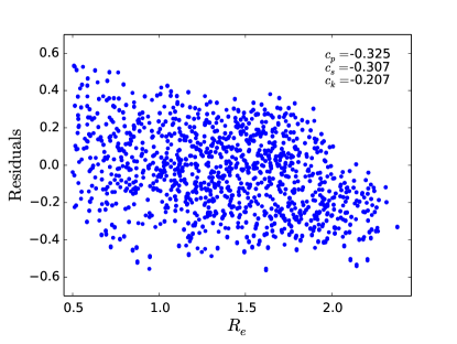
Figure 5: The bulge radius $R_{e}$ versus the residual between our calculated acceleration $g_{{\rm{\scriptscriptstyle SI}}}$ and the MLS2016 relation, shown for $\log(g_{{\rm{\scriptscriptstyle N}}})\approx-11$. The Pearson’s ($c_{p}=-0.325$), Spearman’s ($c_{s}=-0.307$) and Kendall’s ($c_{k}=0.207$) correlation parameters, all with negligible p-values, indicate small correlations. Although they are clear, the correlations do not contribute significantly to the residual width.

7 Discussion and Conclusion

Our findings support the possibility that GR’s self-interaction effects increase the gravitational force in large, non-isotropic mass distributions. When applied to disk galaxies, the increased force on the observed matter transposes to the missing mass needed in the traditional Newtonian analyses. We have thus proposed a plausible explanation for the correlation between the luminous mass in galaxies and their observed gravitational acceleration shown in MLS2016. That this correlation is encapsulated in our models, free of adjustable parameters, indicates its fundamental origin. This work also offers a possible explanation for the MOND acceleration scale $a_{0}$, showing that it dynamically emerges from galaxy baryonic mass distribution. Thus, in our approach, the emergence of $a_{0}$ is due to complexity, rather than new physics, such as modifying gravity or Newton’s dynamical law.

The explanation proposed here is natural in the sense that it is a consequence of the fundamental equations of GR and of the characteristic magnitudes of the galactic gravitational fields, and in the sense that no fine tuning is necessary. This contrasts with the dark matter approach that necessitates both yet unknown particles and a fine tuning in galaxy evolution and baryon-dark matter feedbacks (see e.g. Ludlow et al., 2017). We used several approaches that are quite different, thus leading to a robust conclusion.

The work presented here adds to a set of studies that provide straightforward and natural explanations for the dynamical observations suggestive of dark matter and dark energy, but without requiring them nor modifying the known laws of nature. This includes flat rotation curves of galaxies (Deur, 2009) and the evolution of the universe (Deur, 2019). The Tully-Fisher relation (Tully & Fisher, 1977) also finds an immediate explanation (Deur, 2009). There are compelling parallels between those observations and QCD phenomenology, e.g. the equivalence between galaxies’ Tully-Fisher relation, and hadrons’ Regge trajectories (Deur, 2009, 2017), plausibly due to the similarity between GR’s and QCD’s underlying fundamental equations. The fact that these phenomena are well-known for other areas of nature that possess a similar basic formalism; the current absence of natural and compelling theory for the origin of dark matter (supersymmetry being now essentially ruled out); and the yet unsuccessful direct detection of a dark matter candidate or its production in accelerators despite coverage of the phase-space expected for its characteristics; all support the approach we present here as a credible solution to the missing mass problem.

Appendix A: Parallels between galaxy dynamics, gravitation, and the strong interaction

Quantum chromodynamics (QCD), the gauge theory of the nuclear strong interaction is the archetype of an intrinsic non-linear theory. The non-linearities are intrinsic since they are present even in the pure field case, that is when matter is not present. This contrasts with electromagnetism (QED) which is linear for pure-field and for which non-linearities appear only when matter fields are present. GR possesses the same intrinsic non-linearities as QCD. In fact, the QCD field Lagrangian is topologically equivalent to that of field part of the GR Lagrangian given in Eq. (1). This is seen by developing the standard expression of the QCD Lagrangian density in term of the gluon field strength $F_{\mu\nu}$ as:

$$\mathcal{L}_{\rm QCD} = -\frac{1}{4}F_{\mu\nu}^{a}F^{\mu\nu}_{a}=\frac{1}{4}\big{(}\partial_{\nu}A_{\mu}^{a}-\partial_{\mu}A^{a}_{\nu}\big{)}\big{(}\partial^{\mu}A^{\nu a}-\partial^{\nu}A^{\mu a}\big{)}+\sqrt{\pi\alpha_{s}}f^{abc}\big{(}\partial_{\nu}A_{\mu}^{a}-\partial_{\mu}A_{\nu}^{a}\big{)}A^{\mu b}A^{\nu c}$$

$$- \pi\alpha_{s}f^{abe}f^{cde}A^{a}_{\mu}A^{b}_{\nu}A^{\mu c}A^{\nu d}+{matter~{}term},$$

with $A_{\mu}^{a}$ the gluon field and with the SU(3) color index $a=1,\ldots,8$. $f^{abc}$ are the SU(3) structure constants and $\alpha_{s}$ is the QCD coupling. The $matter~{}term$ is the usual Dirac Lagrangian with a covariant derivative and color indices. With the bracket short-hand notation used for Eq. (1), which now also includes summation over color indices, the QCD Lagrangian has the form:

$$\mathcal{L}_{\rm QCD}=\big{[}\partial A\partial A\big{]}+\sqrt{16\pi\alpha_{s}}\big{[}A^{2}\partial A\big{]}-4\pi\alpha_{s}\big{[}A^{4}\big{]}+\ matter~{}term.$$ (16)

As for GR, the first term is the linear part of the theory and the higher terms are the pure field self-interaction vertices.

While GR and QCD have similar underlying fundamental equations for the pure-field part of their Lagrangians, they also have important differences:

1. GR is a classical field theory while QCD is a quantum field theory;

2. The gravitational field is tensorial (spin-2) while QCD’s field is vectorial (spin-1). Consequently, gravity is always attractive while color charges in QCD can be attracted or repulsed;

3. $G$ is very small ($GM_{p}^{2}=5.9\times 10^{-39}$, with $M_{p}$ the proton mass), while $\alpha_{s}$ is large ($\alpha_{s}\approx 0.1$ at the transition between the weak and strong regimes of QCD (Deur et al., 2016));

However, these differences do not invalidate the parallel between QCD and GR in the context of astronomy.

Regarding difference A, classical effects are usually associated with Feynman tree diagrams, while quantum effects typically emerge from loop diagrams. The latter cause the scale-evolution of the field coupling, while the former generate (in particular) field self-interaction. Thus, quantum effects are necessary for quark confinement since they cause $\alpha_{s}$ to increase enough so that the confinement regime is reached even with only a few color charges involved. However, the scale-evolution of $\alpha_{s}$ is not the basic mechanism for confinement. It is the 3-gluon and 4-gluon interaction tree-diagrams that are at its root. In fact, bound states of QCD can be described semi-classically as divergences of perturbative (i.e. with a finite and relatively small value of the QCD coupling) expansion in ladder-type Feynman diagrams (Dietrich et al., 2013). Other semi-classical approaches to hadronic structure—which is ruled by QCD—exist, such as AdS/QCD (Brodsky et al., 2015), and reproduce efficiently the strong QCD phenomenology (Brodsky et al., 2010). To summarize, while quantum effects are necessary to enable the QCD confinement regime, the underlying mechanism for confinement is arguably classical. GR and QCD Lagrangians have identical tree-diagrams and thus GR, irrespective to its classical nature, should also exhibit effects akin to confinement once its effective field coupling $\sqrt{GM}$ is large enough. In fact, black holes are fully confining solutions of GR.

Differences B and C essentially compensate each other. Classically, a force coupling is truly constant and $G$, in contrast to $\alpha_{s}$, remains small. However, a large effective field coupling can still occur since the magnitudes of the fields are themselves large. They are proportional to $\sqrt{M}$ with $M$ the mass of the field source. This ultimately arises from the tensorial nature of the gravity field, which makes it always attractive: gravitational effects can cumulate into large $M$, such as those characterizing galaxies. This effectively provides the large coupling in lieu of the (quantum) scale-evolution of the coupling. Therefore, the differences B and C balance each other for massive enough systems and self-interaction effects similar to the ones seen in QCD should also occur in massive gravitational systems.

The analogous form of GR and QCD field Lagrangians, and the fact that large effective couplings are possible for both QCD and GR, may explain intriguing similarities between observations suggestive of dark matter and dark energy, and the phenomenology of hadronic structure:

• Just like for hadrons, the total masses of galaxies and galaxy clusters appear much larger than the sum of their known constituent masses.

• Hadrons and galaxies obey similar mass-rotation correlations (Regge trajectories (Regge, 1959) and the Tully-Fisher relation (Tully & Fisher, 1977), respectively); In both case $J\propto M^{\alpha}$ with $J$ the angular momentum, $M$ the (baryonic) mass of the system and $\alpha=1.26\pm 0.07$ or $\alpha=2$ for disk galaxies or hadrons, respectively. (The difference in the value of $\alpha$ is due to the difference in the system symmetry, see (Deur, 2017).)

• The large scale arrangement of galaxies into filaments is reminiscent of QCD strings/flux tubes;

• The nucleon and galaxy matter density profiles both decrease exponentially;

• The approximate compensation at large-scale between dark energy and matter’s gravitational attraction—a phenomenon known as the cosmic coincidence problem—is comparable to the approximate suppression of the strong force at large-distance, i.e. outside the hadron (Deur, 2019).

These parallels and the similar form of QCD and GR’s Lagrangians suggest that very massive structures such as galaxies or cluster of galaxies have entered the non-linear regime of GR, and that phenomena linked to the dark universe may be the consequence of neglecting this regime.

Appendix B: Summary of the method used in the direct calculations

The direct calculation of the effects of field self-interaction based on Eq. (1) employs the Feynman path integral formalism solved numerically on a lattice. While the method hails from quantum field theory, it is applied in the classical limit, see (Deur, 2017). The first and main step is the calculation of the potential between two essentially static ($v\ll c$) sources in the non-perturbative regime. Following the foremost non-perturbative method used in QCD, we employ a lattice technique using the Metropolis algorithm, a standard Monte-Carlo method (Deur, 2009, 2017). The static calculations are performed on a 3-dimensional space lattice (in contrast to the usual 4-dimensional Euclidian spacetime lattice of QCD) using the 00 component of the gravitational field $\varphi_{\mu\nu}$. This implies that the results are taken to their classic limit, as it will be explained below. Furthermore, the dominance of $\varphi_{00}$ over the other components of the gravitational field simplifies Eq (1) in which $\left[\varphi^{n}\partial\varphi\partial\varphi\right]\to a_{n}\varphi_{00}^{n}\partial\varphi_{00}\partial\varphi_{00}$, with $a_{n}$ a set of proportionality constants. One has $a_{0}\equiv 1$ and one can show that $a_{1}=1$ (Deur, 2017).

In this Appendix, we denote $\varphi\equiv\varphi_{00}$ and we will explicitly write $\hbar$ in the expressions in order to identify the quantum effects.

The instantaneous potential from a point-like source located at $x_{1}$ is given at location $x_{2}$ by the two-point Green function $G_{2p}(x_{1}-x_{2})$. In the path-integral formalism,

$$G_{2p}(x_{1}-x_{2})=\frac{1}{Z}\intop\mathrm{D}\varphi\,\varphi(x_{1})\varphi(x_{2})\mathrm{e}^{-\mathrm{i}\,\frac{S_{\mathrm{s}}}{\hbar}},$$ (17)

with $S_{\mathrm{s}}\equiv{\int{\mathrm{d}^{4}x\,\mathcal{L}}}$ the action, $Z\equiv\intop{\mathrm{D}\varphi\,\mathrm{e}^{-\mathrm{i}\,\frac{S_{\mathrm{s}}}{\hbar}}}$, and $\intop{\mathrm{D}\varphi}$ is the sum over all possible field configurations. In the lattice method, $Z\equiv 1$. For Euclidian spacetime lattice simulations, one dimension is the time direction. Suppressing it by considering static or stationary systems allows us to identify $G_{2p}$ to the instantaneous potential. In that case, the sum $\intop{\mathrm{D}\varphi}$ is over configurations in position space only. This allows us to perform standard lattice calculations of difficult forces such as gravity, in spite of its tensorial nature. The method described in the next paragraph is thus the standard one described in lattice textbooks.

$G_{2p}(x_{1}-x_{2})$ is computed numerically on a cubic lattice of $N^{3}$ sites to which a field of value $\varphi$ is associated. The initial values of $\varphi$ at each site is chosen randomly. The ensemble of the $N^{3}$ values is known as a field configuration. A physical configuration should be such that $S_{s}$ is minimized viz the field verifies the Euler-Lagrange equations of motion. To determine numerically these proper configurations, one must first perform a Wick rotation: $\mathrm{e}^{\mathrm{-i}S_{s}/\hbar}\to\mathrm{e}^{-S_{s}/\hbar}$. Euclidean and Minkowski actions being the same, $S_{s}$ remains unchanged. One then follows the Metropolis algorithm iteratively: $S_{s}$ is computed on each sites. The value of $\varphi$ at a given site is randomly varied and the consequent modification $\Delta S_{s}$ is calculated. If $\Delta S_{s}\leq 0$, the new $\varphi$ value tends to minimize $S_{s}$. If so, one retains the new $\varphi$ value since the configuration is now closer to one obeying the equations of motion. If $\Delta S_{s}>0$, one keeps the new $\varphi$ if $\mathrm{e}^{-\Delta S_{s}/\hbar}>\varepsilon$, with $\varepsilon$ randomly chosen between 0 and 1. Otherwise, the new $\varphi$ is rejected. As one iterates the procedure over all the sites, one converges to a configuration following the Euler-Lagrange equations, i.e. the configuration probability distribution obeys $\mathrm{e}^{-S_{s}/\hbar}$. This operation is repeated and the results averaged until they converge and until the statistical uncertainty inherent to the random method becomes small enough. Figure 6 shows an example of calculation which resulted in a linear potential around two forces, viz a constant force.

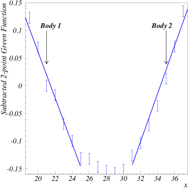
Figure 6: Potential around two massive bodies, with the $1/x$ (free–field, Newtonian case) contribution subtracted. The straight lines demonstrate the approximate linear behavior of the potential away from the mid-distance between the bodies ($x=28$). There, by symmetry, the potential must flatten, as the calculation indeed shows. The potential was calculated in the static limit with Eq. (1) for $n\leq 2$. The two sources are located on the $x-$axis at $d=\pm 7$ lattice spacings $u$ from the lattice center $x=28$, $y=0$ and $z=0$. The coupling is $16\pi GM=5.6\times 10^{-5}~{}u$, the lattice size is $N=85$, the decorrelation parameter (Deur, 2017) is $N_{\mathrm{cor}}=20$ and $N_{\mathrm{s}}=3.5\times 10^{4}$ decorrelated paths were used. As boundary conditions, we used both random field values at the lattice edges, or Dirichlet boundary conditions. The resulting potentials are similar.

The path-integral formalism at the basis of the lattice approach produces intrinsically quantum results. However, the results used in the present manuscript are classical because the lattice time is taken to infinity (Buchmuller & Jakovac, 1998), also known as the high-temperature limit. This can be understood as follow: since the system is static, $S_{\mathrm{s}}\equiv{\int{\mathrm{d}^{4}x\,\mathcal{L}}=\tau S}$, with $S\equiv{\int{\mathrm{d}^{3}x\,\mathcal{L}}}$ and $\tau=\intop_{t_{0}}^{\infty}{\mathrm{d}t\to\infty}$. The exponential of Eq. (17) becomes $\mathrm{e}^{\mathrm{-i}S_{\mathrm{s}}/\hbar}=\mathrm{e}^{\mathrm{-i}\tau S/\hbar}$ and, just like $\hbar\to 0$ suppresses quantum effects, the $\hbar/\tau\to 0$ when $\tau\to\infty$ yields the classical limit.

The method summarized in this appendix has been checked in different ways (Deur, 2017):

• Analytically known potentials for free-field (i.e. theories without self-interacting terms) have been recovered for both massive (Yukawa potential) or massless (Coulomb and Newtonian potentials) fields in three spatial dimensions. They were also satisfactorily verified in the two spatial dimensions case.

• The analytically known potential (Frasca, 2011) for the self-interacting $\phi^{4}$ theory was retrieved.

• The phenomenological static potential for the strong interaction (Cornell potential (Eichten et al., 1975)) was recovered once short distance quantum effects, viz the scale dependence of $\alpha_{s}$, were accounted for.

• The logarithmic potential resulting from the lattice calculation extended from a 2-body system to a thin disk system was also obtained (Deur, 2020) by estimating GR’s self-interaction effects in a typical disk galaxy using a mean-field method that is not based on Eq. (1), see Fig. 7.

Figure 7: Distance dependence of the force obtained using a mean-field approximation to compute the self-interaction effects in a disk galaxy (solid red line) (Deur, 2020). The total galaxy baryonic mass is $M_{\rm tot}=5\times 10^{11}$M_⊙ and has an exponentially decreasing density profile characterized by $h=1.5~{}{\rm kpc}$. The dashed blue line is a parameterization of the force using the same method as for Model 1 described in the manuscript: below a transition scale $r_{t}=2h$, a Newtonian potential ($1/r^{2}$ force) is used and a 2-dimensional logarithmic potential ($1/r$ force) is used. A Fermi-Dirac function ($FD$) of width $r_{t}$ is used to smoothly connect the two domains. $M_{r\leq r_{t}}$ is the mass enclosed within $r_{t}$ and $M_{r\geq r_{t}}=M_{\rm tot}-M_{r\leq r_{t}}$ is the mass outside $r_{t}$. The dashed-dot black line is the expectation from a pure Newtonian potential.

All the GR lattice calculations were done with the Lagrangian given by Eq. (1) with $n=0$, $n\leq 1$ and $n\leq 2$. In the static limit, the ratio of two consecutive field terms $n$ and $n+1$ is $(16\pi GM)^{1/2}\varphi_{00}$, with $16\pi GM$ $\ll 1$ suggesting that Eq. (1) can be truncated at low $n$. The $n=0$ results, which reproduce the expected free-field potentials, differ significantly from the $n\leq 1$ and $n\leq 2$ results once the system mass $M$ is large enough (given the geometry of the system) so that GR has entered its non-linear regime. However, the $n\leq 1$ and $n\leq 2$ calculations yielded similar results, see Fig. 8. Thus, the first self-interaction term ($n=1$) dominates and is enough to describe the effects of field self-interaction. For smaller values of $M$, the $n=0$ contribution to the potential dominates the $n>0$ contributions.

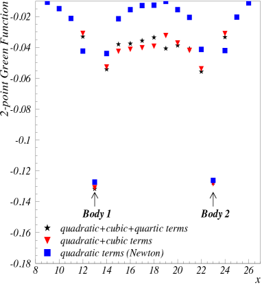
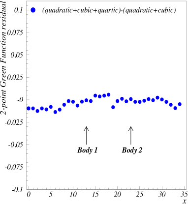
Figure 8: Left: potential between two massive bodies, calculated in the static limit with Eq. (1) for $n\leq 2$ (black stars), $n\leq 1$ (red triangles), and $n=0$ (Newtonian case, blue squares). The two sources are located on the lattice $x-$axis at $\pm 5$ lattice spacings $u$ from the lattice center at $x=18$, $y=0$ and $z=0$. The coupling value is $16\pi GM=1\times 10^{-4}~{}u$, the lattice size $N=35$, the decorrelation parameter (Deur, 2017) $10$ and $N_{\mathrm{s}}=3\times 10^{4}$ decorrelated paths were used. Random field values at the lattice edges were used for boundary conditions (similar results are obtained when using Dirichlet boundary conditions). With these calculation parameters, the difference between the cases $n\leq 2$ and $n\leq 1$ is typically less than 10% of that between the $n=0$ and $n\leq 1$ cases. Right: residual between the potential calculated with $n\leq 2$ for Eq. (1) and the one calculated for $n\leq 1$, shown with the same vertical scale range as that of the left panel for easier comparison. This residual is about $\simeq 10^{-3}$, small compared to the $n\leq 1$ and $n\leq 2$ difference ($4\times 10^{-2}$ between the two bodies), and the potential scale ($0.13$). This justifies the truncation of Eq. (1) to $n=2$.

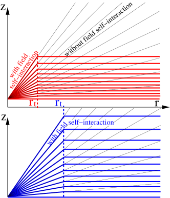
Figure 9: Dependence of $G^{\prime}$ on the transition scale $r_{t}$. Field lines emerge radially for a source (here, for clarity, only those emerging from the galaxy center are shown). A coupling constant, here $G^{\prime}$, determines the density of the field lines emerging from the source (or, in this sketch, the number of field lines represented). Since the field possesses energy-momentum, it interacts gravitationally with itself and with masses. Field self-interactions and interactions of the field with the massive disk in the $z=0$ plane bend the field lines. At smaller $r$ where the field lines are still radially distributed, the force behaves as $1/r^{2}$ (3D regime). At larger $r$ where they are parallel to each others in a given vertical plane, but are still radially distributed in the disk plane—because of the cylindrical symmetry of the disk—the force behaves as $1/r$ (2D regime). For simplicity, the transition distance between the two regimes is shown here to be infinitely short. For a small $r_{t}$ (top panel), the field lines at large $r$ are denser. For a larger $r_{t}$ (bottom panel), the field lines are sparser. Their density is approximately proportional to $r_{t}$. Since a force coupling constant reflects the overall density of its field lines (i.e. ignoring the $r$-dependence) the coupling in the 2D case approximately obeys $G^{\prime}=G/r_{t}$ assumed in this article.

Appendix C: Non-universality of $G^{\prime}$ and its value for infinitely thin disks

The expression of the gravitational force confined in 2D is $G^{\prime}Mm/r$. Therefore, one would naturally expect $G^{\prime}$ to be universal, like $G$ in the 3D case. Furthermore, in the analogous QCD case, the effective coupling $\sigma$ (the analog of $G^{\prime}$), known as the QCD string tension, is indeed universal with a value of $0.18$ GeV² (Deur et al., 2016). However, $G^{\prime}$ is not universal, but depends on the geometry of the galaxy, its mass, and its density distribution.

To understand why, it is convenient to visualize a force as a field flux through an elementary surface. The force coupling constant controls the overall density of the field lines for a unit of charge or mass. Its value does not change the $r$-dependence of the force. Likewise, $G^{\prime}$ determines the overall density of field lines passing through an elementary segment. This density depends on how early the transition from 3D to 2D occurs, as sketched in Fig. 9, where, for clarity, we have drawn only the field lines emerging from the center of the galaxy, its densest locus. The transition occurs early for large disk densities, or can be delayed by the presence of a spherically symmetric bulge. Therefore, $G^{\prime}$ depends on both the morphology and mass distribution of the galaxy components. In the case of an early transition (red lines in Fig. 9), the field lines are denser and $G^{\prime}$ is large. For a later transition (blue lines), the field lines are sparser and $G^{\prime}$ is smaller. Thus, $G^{\prime}$ is not universal and approximately obeys $G^{\prime}=G/r_{t}$.

In the QCD case, $\sigma$ is universal because there is no geometrical or color charge variation: for the heavy meson case to which $\sigma$ applies, two static pointlike sources of unit color charge are invariably considered, with the flavors of the sources and their type of color having no influence on the force. Therefore the same distortion of field lines occurs, regardless of the type of meson considered, and $\sigma$ is universal.

One may also ask what is the value of $G^{\prime}$ for a pure (bulge-less) disk, since there is no bulge-to-disk transition. Inside the disk, the mass distribution is approximately isotropic so the scale height $h_{z}$ of the disk sets a first limit for the scale: one expects $r_{t}\propto h_{z}$. However, considering an infinitely thin disk reveals that a transition scale $r_{t}$ emerges dynamically, which may be larger that $h_{z}$. Even for an infinitely thin disk ($h_{z}=0$), it takes a length $r_{t}$ for the initially radially distributed field lines to bend into parallel field lines. The mass and its distribution thus determine $r_{t}$: the larger the mass and the more concentrated the density, the smaller $r_{t}$. The dynamical emergence of $r_{t}$ in a massive infinitely thin disk is analogous to the emergence of the confinement scale of QCD, or to the energy difference arising between the ground state and first exited levels in atoms or more complex materials in atomic or solid state physics, viz computing $r_{t}$ is a spectral gap problem. The gap problem is notoriously difficult (Carlson et al., 2006) and without known analytical solution. Therefore, even for infinitely thin disks, $r_{t}$—or equivalently $G^{\prime}$—is non-universal and cannot presently be analytically calculated from first principles. It can be obtained from numerical calculations such as those in Refs. (Deur, 2009, 2017), or assessed phenomenologically as done in this article.

References

- Brodsky et al. (2010) Brodsky, S. J., de Teramond, G. F., & Deur, A. 2010, Phys. Rev. D, 81, 096010. arXiv:1002.3948
- Brodsky et al. (2015) Brodsky, S. J., de Teramond, G. F., Dosch, H. G., & Erlich, J. 2015, Phys. Rept., 584, 1, doi: doi:10.1016/j.physrep.2015.05.001
- Buchmuller & Jakovac (1998) Buchmuller, W., & Jakovac, A. 1998, Nucl. Phys. B, 521, 219, doi: doi:10.1016/S0550-3213(98)00215-6
- Caon et al. (1993) Caon, N., Capaccioli, M., & D’Onofrio, M. 1993, MNRAS, 265, 1013, doi: doi:10.1093/mnras/265.4.1013
- Carlson et al. (2006) Carlson, J., Jaffe, A., & Wiles, A. 2006, The Millenium Prize Problems (American Mathematical Society)
- Deur (2009) Deur, A. 2009, Physics Letters B, 676, 21, doi: 10.1016/j.physletb.2009.04.060
- Deur (2014) —. 2014, Monthly Notices of the Royal Astronomical Society, 438, 1535, doi: doi:10.1093/mnras/stt2293
- Deur (2017) —. 2017, Eur. Phys. J. C, 77, 412, doi: doi:10.1140/epjc/s10052-017-4971-x
- Deur (2019) —. 2019, European Physics Journal C, in press, doi: doi:10.1140/epjc/s10052-019-7393-0
- Deur (2020) —. 2020. arXiv:2004.05905
- Deur et al. (2016) Deur, A., Brodsky, S. J., & de Teramond, G. F. 2016, Prog. Part. Nucl. Phys., 90, 1, doi: doi:10.1016/j.ppnp.2016.04.003
- Dietrich et al. (2013) Dietrich, D. D., Hoyer, P., & J rvinen, M. 2013, Phys. Rev. D, 87, 065021
- Eichten et al. (1975) Eichten, E., Gottfried, K., Kinoshita, T., et al. 1975, Phys. Rev. Lett., 34, 369, doi: doi:10.1103/PhysRevLett.34.369
- Einstein et al. (1938) Einstein, A., Infeld, L., & Hoffmann, B. 1938, Annals of Mathematics, 39, 65. http://www.jstor.org/stable/1968714
- Fierz & Pauli (1939) Fierz, M., & Pauli, W. 1939, Proc. Roy. Soc. Lond. A, A173, 211, doi: doi/10.1098/rspa.1939.0140
- Frasca (2011) Frasca, M. 2011, J. Nonlin. Math. Phys., 18, 291, doi: doi:10.1142/S1402925111001441
- Graham & Worley (2008) Graham, A. W., & Worley, C. C. 2008, MNRAS, 388, 1708, doi: doi:10.1111/j.1365-2966.2008.13506.x
- Khosroshahi et al. (2000) Khosroshahi, H. G., Wadadekar, Y., & Kembhavi, A. 2000, The Astrophysical Journal, 533, 162, doi: 10.1086/308654
- Lelli et al. (2017) Lelli, F., McGaugh, S. S., Schombert, J. M., & Pawlowski, M. S. 2017, The Astrophysical Journal, 836, 152, doi: 10.3847/1538-4357/836/2/152
- Ludlow et al. (2017) Ludlow, A. D., Benítez-Llambay, A., Schaller, M., et al. 2017, Phys. Rev. Lett., 118, 161103, doi: doi:10.1103/PhysRevLett.118.161103
- McGaugh et al. (2016) McGaugh, S. S., Lelli, F., & Schombert, J. M. 2016, Phys. Rev. Lett., 117, 201101, doi: doi:10.1103/PhysRevLett.117.201101
- Méndez-Abreu et al. (2008) Méndez-Abreu, J., Aguerri, J. A. L., Corsini, E. M., & Simonneau, E. 2008, A&A, 487, 555, doi: 10.1051/0004-6361:20078089e
- Milgrom (1983) Milgrom, M. 1983, Astrophysical Journal, 270, 365, doi: doi:10.1086/161130
- Padmanabhan (2008) Padmanabhan, T. 2008, Int. J. Mod. Phys. D, 17, 367, doi: doi:10.1142/S0218271808012085
- Regge (1959) Regge, T. 1959, Nuovo Cim., 14, 951, doi: doi:10.1007/BF02728177
- Salam (1974) Salam, A. 1974, in IC/74/55. http://inspirehep.net/record/90219
- Sérsic (1963) Sérsic, J. L. 1963, Boletin de la Asociacion Argentina de Astronomia La Plata Argentina, 6, 41
- Sofue (2015) Sofue, Y. 2015, Publications of the Astronomical Society of Japan, 68, doi: doi:10.1093/pasj/psv103
- Tully & Fisher (1977) Tully, R. B., & Fisher, J. R. 1977, A&A, 54, 661
- Zee (2013) Zee, A. 2013, Einstein Gravity in a Nutshell (Princeton University Press)