Solution of Stokes flow in complex nonsmooth 2D geometries via a linear-scaling high-order adaptive integral equation scheme

Abstract

We present a fast, high-order accurate and adaptive boundary integral scheme for solving the Stokes equations in complex—possibly nonsmooth—geometries in two dimensions. The key ingredient is a set of panel quadrature rules capable of evaluating weakly-singular, nearly-singular and hyper-singular integrals to high accuracy. Near-singular integral evaluation, in particular, is done using an extension of the scheme developed in J. Helsing and R. Ojala, J. Comput. Phys. 227 (2008) 2899–2921. The boundary of the given geometry is “panelized” automatically to achieve user-prescribed precision. We show that this adaptive panel refinement procedure works well in practice even in the case of complex geometries with large number of corners. In one example, for instance, a model 2D vascular network with 378 corners required less than 200K discretization points to obtain a 9-digit solution accuracy.

1 Introduction

Since the pioneering work of Youngren and Acrivos [1, 2], boundary integral equation (BIE) methods have been widely used for studying various particulate Stokes flow systems including drops, bubbles, capsules, vesicles, red blood cells and swimmers (e.g., see recent works [3, 4, 5] and references therein). BIE methods exploit the linearity of Stokes equations and offer several advantages such as reduction in dimensionality, exact satisfaction of far-field boundary conditions, and ease of handling moving geometries. Development of fast algorithms such as the fast multipole methods (FMMs) [6, 7, 8, 9, 10, 11], Ewald summation methods [12, 13, 14, 15], and variants tailored to Stokes equations [16, 17, 18, 19] further extended their scope for solving problems in physically-realistic parameter regimes. Consequently, they are being used to investigate problems in a wide range of physical scales, from microhydrodynamics of isolated particles to large-scale flows generated by suspensions of particles (e.g., see [20, 21, 22]).

Despite their success, many numerical challenges still remain open for BIEs as applied to particulate Stokes flow problems. Prominent among them is the accurate handling of hydrodynamic interactions between surfaces that are almost in contact. For example, in dense suspension flows, the constituent particles often approach very close to each other or to the walls of the enclosing geometries (e.g., see Figure 1). To prevent artificial instabilities in this setting, numerical methods often require adaptive spatial discretizations, accurate nearly-singular integral evaluation schemes (note that while this issue is specific to BIEs, it manifests itself in other forms for other numerical methods) and accurate time-stepping schemes. The primary focus of this paper is addressing the first two issues for two-dimensional problems.

Figure 1: Snapshot from a simulation of bacterial supension flow in a microfluidic chip geometry, which is inspired from the design proposed in [23]. A squirmer model [24] is used for modeling the bacteria, which treats them as rigid bodies with a prescribed slip at the fluid-structure interface. Thereby, we solve the Stokes equations with a no-slip boundary condition on the microfluidic chip geometry, a prescribed tangential velocity on the squirmer boundaries and an imposed parabolic flow profile at the inlet and outlet. We used $730,080$ discretization points for the chip boundary, resulting in $1,460,160$ degrees of freedom, and $128$ discretization points at each of the 120 squirmers. GMRES took about $10$ hours to reach a relative residual of $5.6\times 10^{-8}$, using an $8$-core $3.6$ GHz Intel Core i7 processor with 128 GB of RAM. Color indicates the magnitude of fluid velocity. The estimated PDE relative $L_{2}-$norm error is $2\times 10^{-5}$.

In this work, we introduce specialized panel quadrature schemes that can accurately evaluate layer potentials defined on a smooth open curve, and for target points arbitrarily close to, or on, the curve. This helps the efficient tackling of dense particulate flows constrained in large multiply-connected domains such as in Figure 1. In addition, we formulate a set of rules for refining (or coarsening) the panels used to represent the boundaries, so that a user-specified error tolerance can be achieved automatically. One of the advantages of this adaptive panel refinement procedure is that it can handle geometries with corners (as in Figure 2) or nearly self-touching geometries, using the same quadrature schemes for both weakly- and nearly-singular integrals.

Our work is closely related to two recent efforts, that of Barnett et al. [25] and Ojala–Tornberg [26], both of which, in turn, are extensions to Stokes potentials of the Laplace work of Helsing–Ojala [27]. In [25], three of the co-authors developed high-order global quadrature schemes based on the periodic trapezoidal rule (PTR) for the evaluation of Laplace and Stokes layer potentials defined on a smooth closed planar curve, which achieved spectral accuracy for particles arbitrarily close to each other. Nevertheless, a key limitation of these close evaluation schemes is that they only work for closed curves and have uniform resolution on any part of a curve. Thereby, while they are well-suited for moving rigid and deformable particles immersed in Stokes flow, new machinery is needed for the constraining complex geometries such as those in Figures 1 and 2.

On the other hand, Ojala–Tornberg [26] developed a panel quadrature scheme as done in this work. The main distinction is that [26] uses the BIE framework of Kropinski [28], converting Stokes equations into a biharmonic equation, then tailors it to a specific application (droplet hydrodynamics), whereas our scheme directly tackles all the Stokes layer potentials using physical variables (single-layer, double-layer and their associated pressure and traction kernels). Thereby, it can be integrated with existing BIE methods developed for various physical problems (colloids, drops, vesicles, squirmers and other suspensions) and flow conditions (imposed flow, pressure-, electrically- or magnetically-driven flows, etc) more naturally. We note that resolving nearly-singular integrals is an active area of research owing to its importance in solving several other linear elliptic partial differential equations (PDEs), such as Laplace, Helmholtz and biharmonic equations, via BIEs; other recent works that considered two-dimensional problems include [29, 30, 31, 32, 33, 34].

The predominant class of algorithms for adaptive meshing found in the Stokes BIE literature are the reparameterization schemes (also called the resampling techniques) that are dedicated to resolving boundary mesh distortions arising in deformable particle flow simulations (see [35] for a review on this topic). The primary focus of this work, on the other hand, is to determine an optimal distribution of boundary panels on a given domain so that a user-prescribed tolerance is met when computing the solution. Prior work in this area has mostly been restricted to low-order boundary element methods (BEMs); see [36] for a review. In the last 20 years, high-order $hp$-variants of BEM have been tested for Laplace and Helmholtz problems on polygons (for example [37, 38]). However, we are not aware of any Nyström $hp$-BIEs for the Stokes equations capable of handling arbitrary complex geometries. The recent research of Rachh–Serkh [39] exploits a power-law basis resulting from analysis of the wedge problem to solve Stokes corner problems via a BIE. Here, we take a more pedestrian approach to handling corner singularities via the use of graded meshes. A prototypical example is shown in Figure 2.

The paper is organized as follows. In Section 2, we define the boundary integral operators and state the integral equation formulations for the viscous flow problems considered here. In Section 3, we present the panel quadrature rules for evaluating the Stokes layer potentials. We summarize our algorithm for adaptively discretizing a given geometry in Section 4. We consider several test cases and present results on the performance of our algorithms in Section 5, followed by conclusions in Section 6.

Figure 2: Solution of the Stokes equation in a nonsmooth circular vascular network with Dirichlet boundary condition. We apply no-slip boundary condition at all branch walls, and it is driven by a uniform flow from inner to outer circle. Color here indicates $\log$ of the magnitude of fluid velocity. We used automatically generated panels for both smooth boundaries and $378$ corners, resulting in $356,580$ degrees of freedom. GMRES took about $1$ hour to reach a relative residual of $7.61\times 10^{-11}$ on an $8$-core $4.0$ GHz Intel Core i7 desktop. The PDE solution has a relative $L_{2}-$norm error of $1\times 10^{-9}$. Three high-resolution $\log_{10}$ error plots that correspond to different user-requested tolerance $\epsilon$ near the same reentrant corner are shown on the left; here the short normal lines show panel endpoints, and the black dots quadrature nodes.

2 Mathematical preliminaries

In this section, we first state the PDE formulation for the example shown in Figure 2, reformulate it as a BIE and then discuss the evaluation of the resulting boundary integral operators.

2.1 Boundary value problem and integral equation formulation

The fluid domain $\Omega$ in Figure 2 is a multiply-connected region bounded by $N_{\Gamma}$ closed curves, $\{\Gamma_{i},i=1,\ldots,N_{\Gamma}\}$. Without loss of generality, let $\Gamma_{1}$ be the all-enclosing boundary—i.e., the outer circle in Figure 2—and let $\Gamma=\cup_{i}\Gamma_{i}$. Denoting the fluid viscosity by $\mu$, the velocity by $u$ and the pressure by $p$, the governing boundary-value problem, in the vanishing Reynolds number limit, is

$$-\mu\Delta u+\nabla p=0\quad\text{and}\quad\nabla\cdot u=0 \quad\text{in}\quad\Omega,$$ (1a)

$$u=g \quad\text{on}\quad\Gamma.$$ (1b)

The Dirichlet data $g$ must satisfy the consistency condition $\int_{\Gamma}g\cdot nds=0$, where $n$ is the normal to $\Gamma$. For example, in Figure 2, the flow is driven by an outward flow condition at the inner circle and an inward flow condition at the outer circle. Their magnitude is chosen such that the consistency condition is respected. On the rest of the curves, a no-slip ($g=\bm{0}$) boundary condition is enforced.

While there are many approaches for reformulating the Dirichlet problem (1) as a BIE [40, 41], for simplicity, we use an indirect, combined-field BIE formulation that leads to a well-conditioned and non-rank-deficient linear system. We make the following ansatz:

$$u(x)=\sum_{i=1}^{N_{\Gamma}}\,(\mathbf{S}_{i}\sigma)(x)+(\mathbf{D}_{i}\sigma)(x):=(\mathbf{S}\sigma)(x)+(\mathbf{D}\sigma)(x)\leavevmode\nobreak\ ,\qquad x\in\Omega,$$ (2)

where $\sigma$ is an unknown vector “density” function to be determined, $\mathbf{S}_{i}$ is the velocity Stokes single layer potential (SLP) and $\mathbf{D}_{i}$ is the double layer potential (DLP), defined by

$$(\mathbf{S}_{i}\sigma)(x) =\frac{1}{4\pi\mu}\int_{\Gamma_{i}}\left(I\log\frac{1}{\rho}+\dfrac{r\otimes r}{\rho^{2}}\right)\sigma(y)\,ds_{y}, x\in\Omega,$$ (3)

$$(\mathbf{D}_{i}\sigma)(x) =\frac{1}{\pi}\int_{\Gamma_{i}}\left(\dfrac{r\cdot n_{y}}{\rho^{2}}\dfrac{r\otimes r}{\rho^{2}}\right)\sigma(y)\,ds_{y}, x\in\Omega.$$ (4)

Here, $I$ is the 2-by-2 identity tensor, $r=x-y$, $\rho=\lVert r\rVert_{2}$, and $ds_{y}$ is the arc length element on $\Gamma$. As (2) indicates, we use $\mathbf{S}$ or $\mathbf{D}$ to denote the sum of layer potentials due to all source curves. When combined with their associated pressure kernels (given in the Appendix), the convolution kernels above are fundamental solutions to the Stokes equations (1a); therefore, all that is left to ensure that the ansatz (2) solves the boundary-value problem is to enforce the velocity boundary condition (1b).

We introduce the operator block notation $\mathbb{S}_{ij}\sigma=(\mathbf{S}_{j}\sigma)(\Gamma_{i})$, and similarly $\mathbb{D}_{ij}$ for the double layer potential, i.e., the layer velocity potential restricted to the target curve $\Gamma_{i}$, using the source curve $\Gamma_{j}$. By taking the limit as $x$ approaches $\Gamma$ (from the interior for $\Gamma_{1}$, and exterior for the rest of the curves), the standard jump relations for the single and double layer potentials [40, 41] give the interior case of the following $N_{\Gamma}\times N_{\Gamma}$ BIE system:

$$\left(\begin{bmatrix}I/2&0&\dots\\ 0&I/2&\dots\\ \vdots&\vdots&\ddots\end{bmatrix}+\begin{bmatrix}\eta(\mathbb{S}_{11}+\mathbb{D}_{11})&\mathbb{S}_{12}+\mathbb{D}_{12}&\dots\\ \eta(\mathbb{S}_{21}+\mathbb{D}_{21})&\mathbb{S}_{22}+\mathbb{D}_{22}&\dots\\ \vdots&\vdots&\ddots\end{bmatrix}\right)\begin{bmatrix}\eta\sigma(\Gamma_{1})\\ \sigma(\Gamma_{2})\\ \vdots\end{bmatrix}=\begin{bmatrix}f(\Gamma_{1})\\ f(\Gamma_{2})\\ \vdots\end{bmatrix},\quad\eta=\left\{\begin{array}[]{ll}-1,&\mbox{interior case,}\\ +1,&\mbox{exterior case.}\end{array}\right.$$ (5)

The admixture of SLP and DLP in (2) insures that (5) is of Fredholm second kind, and that interior curves $\Gamma_{i}$, $i=2,3,\dots$ introduce no null-spaces [42, Thm. 2.1] [40, p.128]. Note that the negation of the density for the outer curve (first block column) results in all positive identity blocks. Once we obtain the unknown density function $\sigma$ on $\Gamma$, by solving (5), we can evaluate the velocity at any point in the fluid domain by using 2.

We also consider the exterior boundary-value problem, which can be thought of taking the above outer curve $\Gamma_{1}$ to infinity, removing it from the problem. The fluid domain $\Omega$ becomes the entire plane minus the closed interiors of the other curves; these curves we may relabel as $\Gamma=\cup_{i=1}^{N_{\Gamma}}\Gamma_{i}$. There is also now a given imposed background flow $u_{\infty}(x)$, which in applications is commonly a uniform, shear, or extensional flow. The decay condition $u(x)-u_{\infty}(x)=\bm{\Sigma}\log\|x\|+O(1)$, for some $\bm{\Sigma}\in\mathbb{R}^{2}$, must be appended to (5) to give a well-posed BVP [41]. The representation (2) of the physical velocity is now

$$u(x)=u_{\infty}(x)+(\mathbf{D}\sigma+\mathbf{S}\sigma)(x)\leavevmode\nobreak\ .$$ (6)

The resulting BIE is given as the second case of (5). In the simplest case of physical no-slip boundary conditions, the data in (5) is now $f=-u_{\infty}|_{\Gamma}$, which one may check cancels the velocity on all boundaries.

The close-evaluation schemes of Helsing–Ojala [27] enable efficient and accurate evaluation of certain complex contour integrals arbitrarily close to the boundary, in the case where high order panel-based discretization is used. Thus, a route to evaluate the needed Stokes layer potentials close to the boundary, as in (5) and (2), is to express them in terms of Laplace potentials, which are in turn expressed via contour integrals. The rest of this section presents these formulae.

2.2 Fundamental contour integrals

Let $\tau$ be a given, possibly complex, scalar density function on $\Gamma$. We associate $\mathbb{R}^{2}$ with the complex plane $\mathbb{C}$. Let $n_{y}$ be the outward-pointing unit vector at $y\in\Gamma$, expressed as a complex number. Given a target point $x\in\Omega$, we define the potentials

$$I_{L} =(I_{L}\tau)(x):=\int_{\Gamma}\log|x-y|\tau(y)|dy|=\int_{\Gamma}\log|x-y|\frac{\tau(y)}{in_{y}}dy\leavevmode\nobreak\ ,$$ (real logarithmic) (7)

$$I_{C} =(I_{C}\tau)(x):=\int_{\Gamma}\frac{\tau(y)}{y-x}dy\leavevmode\nobreak\ ,$$ (Cauchy) (8)

$$I_{H} =(I_{H}\tau)(x):=\int_{\Gamma}\frac{\tau(y)}{(y-x)^{2}}dy\leavevmode\nobreak\ ,$$ (Hadamard) (9)

$$I_{S} =(I_{S}\tau)(x):=\int_{\Gamma}\frac{\tau(y)}{(y-x)^{3}}dy\leavevmode\nobreak\ .$$ (supersingular) (10)

Note that, as functions of target point $x$, $I_{C}$, $I_{H}$ and $I_{S}$ are holomorphic functions in $\Omega$, that $(d/dx)(I_{C}\tau)(x)=(I_{H}\tau)(x)$, and $(d/dx)(I_{H}\tau)(x)=2(I_{S}\tau)(x)$. In contrast, $I_{L}$ is not generally holomorphic; yet, for $\tau$ real, $I_{L}$ is the real part of a holomorphic function.

2.3 Laplace layer potentials

Now, let $\tau$ be a real, scalar, density function on $\Gamma$. The Laplace single- and double-layer potentials are defined, respectively, by

$$(\mathcal{S}\tau)(x):=\frac{1}{2\pi}\int_{\Gamma}\left(\log\frac{1}{\rho}\right)\tau(y)ds_{y},\qquad x\in\Omega,$$ (11)

$$(\mathcal{D}\tau)(x):=\frac{1}{2\pi}\int_{\Gamma}\left(\dfrac{\partial}{\partial n_{y}}\log\frac{1}{\rho}\right)\tau(y)ds_{y}=\frac{1}{2\pi}\int_{\Gamma}\left(\frac{r\cdot n_{y}}{\rho^{2}}\right)\tau(y)ds_{y},\qquad x\in\Omega.$$ (12)

In terms of the contour integrals (7) and (8), using $ds_{y}=|dy|=dy/in_{y}$, and the restriction to $\tau$ real, we can rewrite the SLP and DLP as

$$(\mathcal{S}\tau)(x)=\frac{-1}{2\pi}(I_{L}\tau)(x)\quad\text{and}\quad(\mathcal{D}\tau)(x)=\mbox{Re}\,\frac{i}{2\pi}(I_{C}\tau)(x),\quad x\in\Omega.$$ (13)

We will also need the gradients and Hessians of Laplace layer potentials. The gradient of the SLP has components

$$\dfrac{\partial}{\partial x_{1}}(\mathcal{S}\tau)(x)=\dfrac{1}{2\pi}\mbox{Re}\,(I_{C}[\tau/in_{y}])(x),\qquad\dfrac{\partial}{\partial x_{2}}(\mathcal{S}\tau)(x)=\dfrac{-1}{2\pi}\mbox{Im}\,(I_{C}[\tau/in_{y}])(x)\leavevmode\nobreak\ .$$ (14)

The gradient of the DLP requires the Hadamard kernel, and has components

$$\dfrac{\partial}{\partial x_{1}}(\mathcal{D}\tau)(x)=\frac{-1}{2\pi}\mbox{Im}\,(I_{H}\tau)(x),\qquad\dfrac{\partial}{\partial x_{2}}(\mathcal{D}\tau)(x)=\frac{-1}{2\pi}\mbox{Re}\,(I_{H}\tau)(x)\leavevmode\nobreak\ .$$ (15)

The Hessians, which also require $I_{S}$, are discussed in Appendix A.

2.4 Stokes velocity layer potentials

As in [25], we rewrite the Stokes SLP in terms of Laplace potentials, and the DLP in terms of Laplace and Cauchy potentials. Using the identity

$$\dfrac{r\otimes r}{\rho^{2}}\sigma=\dfrac{r}{\rho^{2}}(r\cdot\sigma)=(r\cdot\sigma)\nabla_{x}\log\rho,$$

we can rewrite the Stokes SLP in terms of the Laplace SLP (11) as

$$(\mathbf{S}\sigma)(x)\;= {1\over 4\pi\mu}\Big{\{}\int_{\Gamma}\left(\log\frac{1}{\rho}\right)\,\sigma ds_{y}+\nabla\int_{\Gamma}\left(\log\frac{1}{\rho}\right)\,(y\cdot\sigma)ds_{y}$$ (16)

$$-x_{1}\nabla\int_{\Gamma}\left(\log\frac{1}{\rho}\right)\,\sigma_{1}ds_{y}-x_{2}\nabla\int_{\Gamma}\left(\log\frac{1}{\rho}\right)\,\sigma_{2}ds_{y}\Big{\}}\leavevmode\nobreak\ ,$$

where $\nabla=\nabla_{x}$ is assumed from now on. Therefore, three Laplace potentials (and their first derivatives) with real scalar density functions $y\cdot\sigma$, $\sigma_{1}$, and $\sigma_{2}$ need to be computed to evaluate the Stokes SLP. Similarly, using the identity

$$\nabla\left(\dfrac{r\cdot n_{y}}{\rho^{2}}\right)=\dfrac{n_{y}}{\rho^{2}}-(r\cdot n_{y})\dfrac{2r}{\rho^{4}}\leavevmode\nobreak\ ,$$ (17)

the Stokes DLP can be written as

$$(\mathbf{D}\sigma)(x)\;= {1\over 2\pi}\int_{\Gamma}{n_{y}\over\rho^{2}}(r\cdot\sigma)ds_{y}+{1\over 2\pi}\nabla\int_{\Gamma}{r\cdot n_{y}\over\rho^{2}}(y\cdot\sigma)ds_{y}$$ (18)

$$-{1\over 2\pi}x_{1}\nabla\int_{\Gamma}{r\cdot n_{y}\over\rho^{2}}\sigma_{1}ds_{y}-{1\over 2\pi}x_{2}\nabla\int_{\Gamma}{r\cdot n_{y}\over\rho^{2}}\sigma_{2}ds_{y}\leavevmode\nobreak\ .$$

While the last three terms are gradients of Laplace DLPs, the first term requires a Cauchy integral. More concisely, we can write (16) and (18) as

$$(\mathbf{S}\sigma)(x) =\frac{1}{2\mu}\Big{(}\,(\mathcal{S}\sigma_{1},\mathcal{S}\sigma_{2})+\nabla\mathcal{S}[y\cdot\sigma]-x_{1}\nabla\mathcal{S}\sigma_{1}-x_{2}\nabla\mathcal{S}\sigma_{2}\Big{)}(x), x\in\Omega,$$ (19)

$$(\mathbf{D}\sigma)(x) =\Big{(}\,\frac{1}{2\pi}\text{Re}\,\big{(}I_{C}(\tau_{1}),I_{C}(\tau_{2})\big{)}+\nabla\mathcal{D}[y\cdot\sigma]-x_{1}\nabla\mathcal{D}\sigma_{1}-x_{2}\nabla\mathcal{D}\sigma_{2}\Big{)}(x), x\in\Omega,$$ (20)

where, as above, a pair $(\cdot,\cdot)$ indicates two vector components, and a short calculation verifies that the complex scalar density functions $\tau_{1}$ and $\tau_{2}$

$$\tau_{1}=(\sigma_{1}+i\sigma_{2})\frac{\text{Re}\,n_{y}}{n_{y}},\qquad\tau_{2}=(\sigma_{1}+i\sigma_{2})\frac{\text{Im}\,n_{y}}{n_{y}},$$ (21)

where $n_{y}$ is interpreted as a complex number, makes the identity hold (i.e. the first term in (20) equals the first term in (18)).

In summary, the procedure discussed in this section enables us to express the velocity field anywhere in the fluid domain, represented by (2), in terms of fundamental contour integrals. Similar formulae exist for the fluid pressure and hydrodynamic stresses, which are commonly needed in several applications; we present these in Appendix A.

3 Nyström discretization and evaluation of layer potentials

3.1 Overview: discretization and the plain Nyström formula

Firstly, we need to specify a numerical approximation of the density function $\sigma$. For simplicity, consider the case of an exterior BVP on a single closed curve $\Gamma$ parameterized by $Z:[0,2\pi)\to\mathbb{R}^{2}$, such that $\Gamma=Z([0,2\pi))$. The Stokes BIE (5) is then

$$(I/2+\mathbb{K})\sigma=f,\qquad\mathbb{K}:=\mathbb{D}+\mathbb{S}\leavevmode\nobreak\ ,$$ (22)

where $\sigma$ and $f$ are 2-component vector functions on $\Gamma$.

Given the user requested tolerance $\epsilon$, the boundary is split into $n_{\Lambda}$ disjoint panels $\Lambda_{i}$, $i=1,\ldots,n_{\Lambda}$ using the adaptive algorithm to be described in Section 4. Each panel will have $p$ nodes, giving $N=pn_{\Lambda}$ nodes in total, hence $2N$ density unknowns. The $i$th panel is $\Lambda_{i}=Z([a_{i-1},a_{i}])$, where $a_{i}$, $i=0,\dots,n_{\Lambda}$ are the parameter breakpoints of all panels (where $a_{n_{\Lambda}}\equiv a_{0}(\mbox{mod }2\pi)$). Let the $p$-point Gauss–Legendre nodes and weights on the parameter interval $[a_{i-1},a_{i}]$ be $t^{(i)}_{j}$ and $w^{(i)}_{j}$ respectively, for $j=1,\dots,p$. Then, for smooth functions $f$ on $\Gamma$, the quadrature rule

$$\int_{\Gamma}f(y)ds_{y}=\int_{0}^{2\pi}f(Z(t))\,|Z^{\prime}(t)|\,dt\;\approx\;\sum_{i=1}^{n_{\Lambda}}\sum_{j=1}^{p}f(Z(t^{(i)}_{j}))\,|Z^{\prime}(t^{(i)}_{j})|\,w^{(i)}_{j}=:\sum_{\ell=1}^{N}f(y_{\ell})\,|Z^{\prime}(t_{\ell})|\,w_{\ell}$$ (23)

holds to high-order accuracy. In the last formula above $\{t_{\ell}\}_{\ell=1}^{N}$ denotes the entire set of parameter nodes, $y_{\ell}=Z(t_{\ell})$ their images on $\Gamma$, and $w_{\ell}$ their corresponding weights.

The Nyström method [43, Sec. 12.2] is then used to approximately solve the BIE (22). Broadly speaking, this involves substituting the quadrature rule (23) for the integral implicit in the BIE, then enforcing the equation at the quadrature nodes themselves. The result is the $2N$-by-$2N$ linear system,

$$\bm{A}\bm{\sigma}=\mathbf{f}$$ (24)

where $\mathbf{f}:=\{f(t_{\ell})\}_{\ell=1}^{N}$ is the vector of 2-component values of the right-hand side $f$ at the $N$ nodes, and $\bm{\sigma}:=\{\sigma_{\ell}\}_{\ell=1}^{N}$ is the vector of 2-component densities at the $N$ nodes. $\bm{A}=\{A_{ij}\}_{i,j=1,\dots,n_{\Lambda}}$ is a $n_{\Lambda}\times n_{\Lambda}$ block matrix, where each block $A_{ij}$ is a $2p\times 2p$ submatrix that represents the interaction from source panel $\Lambda_{j}$ to target panel $\Lambda_{i}$. For targets that are “far” (in a sense discussed below) from a given source panel, the formula for filling corresponding elements of $\bm{A}$ is simple. Letting the index be $\ell$ for such a target node, and $\ell^{\prime}$ for a source lying in such a panel, using the smooth rule (23) gives the matrix element

$${\bm{A}}_{\ell,\ell^{\prime}}\;=\;K(y_{\ell},y_{\ell^{\prime}})\,|Z^{\prime}(t_{\ell^{\prime}})|\,w_{\ell^{\prime}}\leavevmode\nobreak\ ,\qquad\mbox{(Nystr\"{o}m rule for $y_{\ell}$ ``far'' from panel containing $y_{\ell^{\prime}}$)}$$ (25)

where $K(x,y)=S(x,y)+D(x,y)$, the latter being the kernels appearing in (3)–(4). Recall that each element in (25) is a $2\times 2$ tensor, since $K$ is. This defines the plain (smooth) rule for matrix elements (note that we need not include the diagonal $I/2$ from (22) since $\ell=\ell^{\prime}$ is never a “far” interaction).

Sections 3.2–3.4 will be devoted to defining “close” vs “far” and explaining how “close” matrix elements are filled. Assuming for now that this has been done, the result is a dense matrix $A$ that is well-conditioned independent of $N$, because the underlying integral equation is of Fredholm second kind. Then an iterative solver for (24), such as GMRES, will converge rapidly. The result is the vector $\bm{\sigma}$ approximating the density at the nodes. Assuming that (24) has been solved exactly, there is still a discretization error, whose convergence rate is known to inherit that of the quadrature scheme applied to the kernel [43, Sec. 12.2]. Given this, the density function may be evaluated at any point $y\in\Gamma$ using either the Nyström interpolant (which is global and hence inconvenient), or local $p$th-order Lagrange interpolation from just the points on the panel in which $y$ lies. When needed, we will use the latter. The generalization of the above Nyström method to multiple closed curves is clear.

Remark 1.

When the problem size is large, the matrix-vector multiplication in (24), which requires $O(N^{2})$ time, can be rapidly computed using the fast multipole methods (FMM) in only $O(N)$ time. This is because all but $O(N)$ of the matrix elements involve the plain rule (25), for which applying the matrix is equivalent to evaluation of a potential with weighted source strengths. In our large examples (Figures 1 and 2), we use an OpenMP-parallelized Stokes FMM code due to Rachh, built upon the Goursat representation of the biharmonic kernel [44, 45].

Finally, once $\bm{\sigma}$ has been solved for, the evaluation of the velocity $u(x)$ at arbitrary targets $x\in\Omega$ is possible, by approximating the representation (2) or (6), as appropriate. By linearity, this breaks into a sum of contributions from each source panel on each curve, which may then be handled separately. Thus a given target $x\in\Omega$ may, again, fall “far” or “close” to a given source panel (denoted by $\Lambda=Z([a,b])$). If it is “far” (according to the same criterion as for matrix elements), then a simple plain rule is used. Letting $u_{\Lambda}$ be the contribution to $u$ from source panel $\Lambda$, this rule arises, as with (25), simply by substituting (23) into the representation, giving

$$u_{\Lambda}(x)=\int_{\Lambda}K(x,y)\sigma(y)ds_{y}\approx\sum_{j=1}^{p}K(x,y_{j})\,|Z^{\prime}(t_{j})|\,w_{j}\sigma_{j}\leavevmode\nobreak\ ,\qquad\mbox{(evaluation rule for $x$ ``far'' from $\Lambda$)}$$ (26)

where $y_{j}:=Z(t_{j})$ are the nodes, and $\sigma_{j}:=\sigma(y_{j})$ the 2-component density values, belonging to $\Lambda$. For large $N$, the FMM is ideal for the task of evaluating $u$ at many targets, using this plain rule. An identical quadrature rule may be applied to the representations in the Appendix to evaluate pressure and traction at $x$.

3.2 Close-evaluation and self-evaluation corrections

If a target (on-surface node or off-surface evaluation point) is close enough to a source panel that (25) is inaccurate, a new close-evaluation formula is needed. A special case is when the target is a node from the source panel itself, which we call self-evaluation. The integrand is nearly singular for close-evaluation and singular for self-evaluation; in the latter case, the integral is understood as an improper integral (SLP) or a principal value integral (DLP). Conveniently, we will use the same rule for self-evaluation as both on-surface and off-surface close-evaluation (this contrasts much prior work, where the self-evaluation used another set of tailored high-order integration schemes; see, e.g., [46]).

We quantify “close” and “far” as follows. Given a panel $\Lambda_{j}=Z([a,b])$, a target point $x$ is close to $\Lambda_{j}$ if it lies inside the ellipse

$$|z-Z(a)|+|z-Z(b)|=C\,S,$$ (27)

otherwise $x$ is far from $\Lambda_{j}$. A panel $\Lambda_{i}$ is close to $\Lambda_{j}$ if any point $z\in\Lambda_{i}$ lies inside the ellipse (27), otherwise $\Lambda_{i}$ is far from $\Lambda_{j}$. (Note that $\Lambda_{j}$ is close to itself.) In (27), $S$ is the arc length of $\Lambda_{j}$ and $C>1$ is a constant. For the numerical examples in Section 5 we have picked $C=2.5$, which is large enough to include all of both neighboring panels of $\Lambda_{j}$ most of the time.

The rationale for the above heuristic is based upon the accuracy of the plain rule (26) (and its corresponding matrix element rule (25)). Examining (23), if the integrand $f(Z(t))|Z^{\prime}(t)|$ is analytic with respect to $t$ within a Bernstein ellipse (for the parameter domain $[a_{j-1},a_{j}]$ for this panel) of size parameter $\varrho>1$, then the error convergence for the Gauss–Legendre rule for this panel is $O(\varrho^{-2p})$, i.e. exponential in the panel degree $p$ [47, Theorem 19.3]. Since in our case $f(Z(t))=K(x,Z(t))\sigma(Z(t))$, and $K(x,y)$ is analytic for $x\neq y$, for such analyticity of the integrand, $x$ must be outside the image of this Bernstein ellipse under $Z$. In the case where the panel is approximately flat, this image is approximated by the ellipse with foci $Z(a)$ and $Z(b)$, which gives the above geometric “far” criterion. The choice of $C$ is empirically made to achieve an exponential error convergence rate in $p$ no worse than that due to the next-neighboring panels discussed in Stage 1 of Section 4, in the case of panel shapes produced by the procedure in that section. Note that $\sigma(Z(t))$ must also be assumed to be analytic in the ellipse; we expect this to hold again because the panels will be sufficiently refined. For a more detailed error analysis of the plain panel rule using the Bernstein ellipse, see [48, Sect. 3.1].

So far we have presented (only in the “far” case) formulae for both filling Nyström matrix elements (25), and for evaluation of the resulting velocity potential (26). We now make the point that, in both the “far” and “close” cases, these are essentially the same task.

Remark 2 (Matrix-filling is potential evaluation).

The matrix element formula (25) is just a special case of the evaluation formula (26) for the on-surface target $x=y_{\ell}$, and with a Kronecker-delta density $\sigma_{j}=\delta_{j,\ell^{\prime}}$. I.e., one can compute (the “far” contributions to) $\bm{A}\bm{\sigma}$ from $\bm{\sigma}$, as needed for each iteration in the solution of (24), simply via the evaluation formula (26) with targets $x$ as the set of nodes $\{y_{\ell}\}$. This will also apply to the special “close” formulae presented below. Henceforth we now present only formulae for evaluation; the corresponding matrix element formulae are easy to extract (see Section 3.4)

Note that the diagonal blocks $A_{ii}$ when computed using the special close-evaluation quadratures will implicitly include the $I/2$ jump relation appearing in (22).

Finally, to accelerate the computation, the close- and self-evaluations can be precomputed as matrices (see Section 3.4) from which the (inaccurate) matrices involving the plain rule (25) are subtracted. The resulting “correction matrix” blocks are assembled and stored as a $2N$-by-$2N$ sparse matrix. The entire application of $\bm{A}$ to the density vector is then performed using the FMM with the plain rule (25), plus the action of this sparse matrix to replace the “close” interactions with their accurate values. This application is used to solve the whole linear system iteratively. We do this for our large-scale examples in Section 5.

3.3 Close-evaluation of potentials

Since we will perform all Nyström matrix filling using the same formulae as for close-evaluation of potentials (on- or off-surface), we now present formulae for the close-evaluation task. As before, we consider a single target point $x\in\Omega$ which is “close” to the single source panel $\Lambda=Z([a,b])$, on which a density $\sigma_{j}$ is known at the nodes $j=1,\dots,p$. Recall that the $p$-point Gauss–Legendre nodes and weights for the parameter interval $[a,b]$ are $t_{j}$ and $w_{j}$.

We adapt special panel quadratures proposed for the Laplace case by Helsing and Ojala [27]. They use high-order polynomial interpolation in the complex plane to approximate the density function, then apply a recursion to exactly evaluate the near-singular integral for each monomial basis function. In Section 2 we showed that all the needed Stokes potentials may be written in terms of $I_{L}(x)$, $I_{C}(x)$, $I_{H}(x)$ and $I_{S}(x)$ from (7)–(10), involving scalar Cauchy densities $\tau$ derived from the given Stokes density $\sigma$. Thus in the following subsections we need only cover close-evaluation of each contour integral in turn. Although much of this is known [27], there are certain implementation details and choices that make a complete distillation valuable.

It turns out that the Helsing–Ojala polynomial approximation is most stable when assuming that $Z(a)=1$ and $Z(b)=-1$, i.e. the panel endpoints are $\pm 1$ in the complex plane. Thus we start by making this assumption, then in Sec. 3.3.4 show how to correct the results for a panel with general endpoints.

Recall that $\sigma$, hence the derived scalar functions $\tau$ needed in the contour integrands, is available only at the $p$ nodes of $\Lambda$. In order to improve the accuracy of the complex approximation for bent panels, firstly an upsampling is performed to $m>p$ “fine” nodes, using Lagrange interpolation in the parameter $t\in[a,b]$ from the $p$ nodes to the $m$ fine nodes. We find that $m=2p$ is beneficial without incurring significant extra cost. Let $\tilde{\tau}_{j}$, $j=1,\dots,m$ denote the fine density values, and $z_{j}=Z(\tilde{t}_{j})\in\Lambda$ be the fine nodes, where $\tilde{t}_{j}$ and $\tilde{w}_{j}$ are the $m$-point Gauss–Legendre nodes and weights respectively for $[a,b]$. The following schemes now will use only the fine values and nodes.

3.3.1 Close evaluation of the Cauchy potential

We approximate $\tau$ on the panel $\Lambda$ in the complex variable by the degree $m-1$ polynomial

$$\tau(y)\approx\sum_{k=1}^{m}a_{k}y^{k-1},\qquad y\in\Lambda\leavevmode\nobreak\ .$$ (28)

The vector of coefficients $\mathbf{a}:=\{a_{k}\}_{k=1}^{m}$ is most conveniently found by using a dense direct solve of the square Vandermonde system

$$V\mathbf{a}=\tilde{\bm{\tau}}\leavevmode\nobreak\ ,$$ (29)

with elements $V_{jk}=z_{j}^{k-1}$, $j,k=1,\dots,m$, and right hand side $\tilde{\bm{\tau}}:=\{\tilde{\tau}_{j}\}_{j=1}^{m}$. It is known that, for any arrangement of nodes $z_{j}$ other than those very close to the roots of unity, the condition number of $V$ grows exponentially with $m$ [49]. However, as discussed in [27, App. A], at least for $m<50$, despite the extreme ill-conditioning, backward stability of the linear solver insures that the resulting polynomial matches the values at the nodes to close to machine precision. For this we use MATLAB mldivide which employs standard partially-pivoted Gaussian elimination.

The remaining step is to compute the contour integral of each monomial,

$$p_{k}=p_{k}(x):=\int_{-1}^{1}\frac{y^{k-1}}{y-x}dy,\quad k=1,\ldots,m\leavevmode\nobreak\ ,$$ (30)

which are, recalling (8), then combined using (28) to get

$$I_{C}\;\approx\;\sum_{k=1}^{m}a_{k}p_{k}\leavevmode\nobreak\ .$$ (31)

By design, since the monomials are with respect to $y$ in the complex plane (as opposed to, say, the parameter $t$), Cauchy’s theorem implies that each $p_{k}$ is independent of the curve $\Lambda$ and depends only on the end-points. Specifically, for $k=1$ we may integrate analytically by deforming $\Lambda$ to the real interval $[-1,1]$, so

$$p_{1}\;:=\;\int_{-1}^{1}\frac{1}{y-x}dy\;=\;\log(1-x)-\log(-1-x)\pm 2\pi i{\mathcal{N}}_{x}$$ (32)

where ${\mathcal{N}}_{x}\in\mathbb{Z}$ is an integer winding number that depends on the choice of branch cut of the log function. For the standard cut on the negative real axis then ${\mathcal{N}}_{x}=0$ when $x$ is outside the domain enclosed by the oriented curve composed of $\Lambda$ traversed forwards plus $[-1,1]$ traversed backwards, ${\mathcal{N}}_{x}=+1$ ($-1$) when $x$ is inside a region enclosed counterclockwise (clockwise) [27]. However, since it is inconvenient and error-prone to decide ${\mathcal{N}}_{x}$ for points on or very close to $\Lambda$ and $[-1,1]$, we prefer to combine the two logs then effectively rotate its branch cut by a phase $\phi\in\mathbb{R}$, by using

$$p_{1}\;=\;i\phi+\log\frac{1-x}{e^{i\phi}(-1-x)}\leavevmode\nobreak\ ,$$ (33)

where $\phi=-\pi/4$ when the upwards normal of the panel points into $\Omega$ (as for an interior curve), or $\phi=\pi/4$ otherwise. This has the effect of pushing the branch cut “behind” the panel (away from $\Omega$; see Fig. 3), with the cut meeting $\pm 1$ at an angle $\phi$ from the real axis. The potential is correct in the closure of $\Omega$, including on the panel itself, without any topological tests needed (hence the unified handling of close and self evaluations in Sec. 3.2). This can fail if a panel is very curved (such a panel would be inaccurate anyway), or if a piece of $\Omega$ approaches close to the back side of the panel (which can be prevented by adaptive refinement as in Section 4). In practice we find that this is robust. However, we will mention one special situation where (33) could fail and therefore careful adjustment of the branch cut is critical; see Remark 3 below.

The following 2-term recurrence is easy to check by adding and subtracting $xy^{k-1}$ from the numerator of the formula (30) for $p_{k+1}$:

$$p_{k+1}=xp_{k}+(1-(-1)^{k})/k\leavevmode\nobreak\ .$$ (34)

For $|x|<1.1$ we find that the recurrence is sufficiently stable to use upwards from the value $p_{1}$ computed by (33), to get $p_{2},\dots,p_{m}$. However, for targets outside this close disc, especially for larger $m$, the upwards direction is unstable. Thus, here instead we use numerical quadrature on (30) to get

$$p_{m}\approx\sum_{j=1}^{m}\frac{z_{j}^{m-1}}{z_{j}-x}Z^{\prime}(\tilde{t}_{j})\tilde{w}_{j}\leavevmode\nobreak\ ,$$ (35)

then apply (34) downwards to compute $p_{m-1},\dots,p_{2}$, and as before use $p_{1}$ from (33). Outside of the disc, no branch cut issues arise.

Remark 3 (branch cuts at corners).

When a panel $\Lambda$ is directly touching a corner, directly applying (33) can fail no matter how much the panels are refined. In Figure 3a, the panel on the opposite side of the corner, $\Lambda^{\prime}$, is always behind $\Lambda$ and lying across the branch cut associated to $\Lambda$. Consequently, the close evaluation from $\Lambda$ to $\Lambda^{\prime}$ results in completely wrong values, also leading to ill-conditioning of the whole system (24). Instead, one can simply change the sign of $\phi$ in (33) to flip the branch cut to accommodate the targets on $\Lambda^{\prime}$ (Figure 3b). In practice, we find that this is robust for corners of arbitrary angles.

(a)	(b)

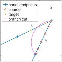
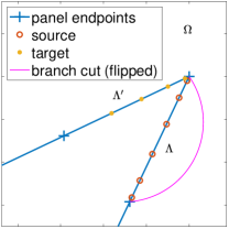
Figure 3: Special handling of close evaluation branch cut when the panel is touching a reentrant corner. (a) The target panel $\Lambda^{\prime}$ is crossing the branch cut of the source panel $\Lambda$ defined by (33), resulting in wrong close evaluation values. (b) Changing the sign of $\phi$ in (33) flips the branch cut to the other side; close evaluation at the targets are now correct.

3.3.2 Close evaluation of the logarithmic potential

For $\tau$ real, we can write the final form in (7) as

$$I_{L}\;=\;\mbox{Re}\int_{\Lambda}\log(y-x)\frac{\tau(y)}{in_{y}}dy,$$ (36)

which shows that the quantity to approximate on $\Lambda$ as a complex polynomial is $\tau(y)/in_{y}$. Thus we find the coefficients in

$$\frac{\tau(y)}{in_{y}}\;\approx\;\sum_{k=1}^{m}b_{k}y^{k-1},\qquad y\in\Lambda\leavevmode\nobreak\ ,$$ (37)

by solving (29) but with modified right hand side $\{\tilde{\tau}_{j}/in_{z_{j}}\}_{j=1}^{m}$. Defining

$$q_{k}\;:=\;\int_{-1}^{1}y^{k-1}\log(y-x)dy,\quad k=1,\ldots,m$$ (38)

then (37) gives

$$\int_{-1}^{1}\log(y-x)\frac{\tau(y)}{in_{y}}dy\;\approx\;\sum_{k=1}^{m}b_{k}q_{k}\leavevmode\nobreak\ ,$$ (39)

whose real part is $I_{L}$. Each $q_{k}$ is computed from $p_{k}$ of (30) as evaluated in Sec. 3.3.1, via a formula easily proven by integration by parts,

$$q_{k}=\frac{-p_{k+1}+\log(1-x)-(-1)^{k}\log(1+x)}{k}=\begin{cases}\bigl{(}-p_{k+1}+i\phi+\log\frac{1-x}{e^{i\phi}(-1-x)}\bigr{)}/k\leavevmode\nobreak\ ,&k\mbox{ even },\\ \bigl{(}-p_{k+1}+\log[(1-x)(-1-x)]\bigr{)}/k\leavevmode\nobreak\ ,&k\mbox{ odd },\\ \end{cases}$$ (40)

where the latter form is that used in the code, needed to match the branch cut rotation used for $p_{k}$ in (33). The final evaluation of $I_{L}$ is then via

$$I_{L}\;\approx\;\mbox{Re}\sum_{k=1}^{m}b_{k}q_{k}\leavevmode\nobreak\ .$$ (41)

3.3.3 Close evaluation of the Hadamard and supersingular potentials

The double-layer Stokes velocity requires gradients of Laplace potentials (15), which require $I_{H}$. Also, the traction of the Stokes single-layer (51) involves $I_{H}$ applied to $\tau(y)/in_{y}$, and the traction of the Stokes double-layer further involves $I_{S}$ (Appendix A).

Using the complex monomial expansion (28), we have

$$I_{H}\;\approx\;\sum_{k=1}^{m}a_{k}r_{k},\hskip 72.26999ptI_{S}\;\approx\;\sum_{k=1}^{m}a_{k}s_{k},$$ (42)

where

$$r_{k}\;:=\;\int_{-1}^{1}\frac{y^{k-1}}{(y-x)^{2}}dy,\hskip 36.135pts_{k}\;:=\;\int_{-1}^{1}\frac{y^{k-1}}{(y-x)^{3}}dy,\qquad k=1,\ldots,m\leavevmode\nobreak\ .$$ (43)

The following formulae can be shown by integration by parts, and enable $r_{k}$ and $s_{k}$ to be found,

$$r_{k}=(k-1)p_{k-1}+\frac{(-1)^{k-1}}{-1-x}-\frac{1}{1-x}\leavevmode\nobreak\ ,\qquad s_{k}=\frac{k-1}{2}r_{k-1}+\frac{(-1)^{k-1}}{2(-1-x)^{2}}-\frac{1}{2(1-x)^{2}}\leavevmode\nobreak\ ,$$ (44)

using $p_{k}$ from (30) as computed in Sec. 3.3.1, and $p_{0}=0$.

3.3.4 Transforming for general panel endpoints

To apply close-evaluation methods in the above three sections to a general panel $\Lambda=Z([a,b])$, define the complex scale factor $s_{0}:=(Z(b)-Z(a))/2$ and origin $x_{0}=(Z(b)+Z(a))/2$. Then the affine map

$$x=s(\tilde{x}):=\frac{\tilde{x}-x_{0}}{s_{0}}$$

takes any target $\tilde{x}$ to its scaled version $x$. Likewise, the fine nodes are scaled by $z_{j}=s(Z(\tilde{t}_{j}))$, and the factor $Z^{\prime}$ in (35) is replaced by $Z^{\prime}/s_{0}$. Following Sec. 3.3.1 using these scaled target and fine nodes, no change in the result $I_{C}$ is needed. However, the value of $I_{H}$ computed in Sec. 3.3.3 must afterwards be divided by $s_{0}$, and the value of $I_{S}$ divided by $s_{0}^{2}$. The value of $I_{L}$ computed in Sec. 3.3.2 must be multiplied by $|s_{0}|$, and then have $|Z^{\prime}(\tilde{t}_{j})w_{j}/s_{0}|\log|s_{0}|$ subtracted.

3.4 Computation of close-evaluation matrix blocks

The above described how to evaluate $(I_{L}\tau)(x)$, $(I_{C}\tau)(x)$, $(I_{H}\tau)(x)$ and $(I_{S}\tau)(x)$ given known samples $\tilde{\tau}_{j}$ at a panel’s fine nodes. In practice it is useful to instead precompute a matrix block $A$ which takes any density values at a panel’s original $p$ nodes $y_{j}$ to a set of $n$ target values of the contour integral. Consider the case of the Cauchy kernel, and let $A$ denote this $n$-by-$p$ matrix. Let $L$ be the $m$-by-$p$ Lagrange interpolation matrix from the nodes $t_{j}$ to fine nodes $\tilde{t}_{j}$, which need be filled once and for all. Let $P$ be the $n$-by-$m$ matrix with entries $P_{ik}=p_{k}(x_{i})$, given by (30), where $\{x_{i}\}_{i=1}^{n}$ is the set of desired targets. In exact arithmetic one has

$$A=PV^{-1}L\leavevmode\nobreak\ .$$

However, since $V$ is very ill-conditioned, filling $V^{-1}$ and using it to multply to the right is numerically unstable. Instead an adjoint method is used: one first solves the matrix equation $V^{\top}X=P^{\top}$, where $\top$ indicates non-conjugate transpose, then forms the product

$$A=X^{\top}L\leavevmode\nobreak\ .$$

The matrix solve is done in a backward stable fashion via MATLAB’s mldivide. A further advantage of the adjoint approach is that if $n$ is small, the solve is faster than computing $V^{-1}$.

The formulae for the logarithmic, Hadamard and supersingular kernels are analogous.

4 Adaptive panel refinement

In order to solve a BIE to high accuracy, it is necessary to set up panels such that the given complex geometry is correctly resolved. In this section, we describe a procedure that adaptively refine the panels based solely on the geometric properties. Specifically, our refinement algorithms take into account the accuracy of geometric representations (including arc length and curvature), the location of corners, and the distance between boundary components. It necessarily has some ad-hoc aspects, yet we find it quite robust in practice.

Suppose that for a user-prescribed tolerance $\epsilon$, the goal is to find a partition $\Gamma=\bigcup\limits_{i=1}^{n_{\Lambda}}\Lambda_{i}$ such that the error, $\varepsilon$, of evaluating boundary integral operators such as (22) satisfies $\varepsilon\lessapprox\epsilon$. To this end, we describe our adaptive refinement scheme which proceeds with three stages. In what follows, we again assume that the panel under consideration $\Lambda=Z([a,b])$ is rescaled such that its two endpoints are $\pm 1$.

Stage 1: Choice of overall $p$.

Given tolerance $\epsilon$, the goal is to determine a number of quadrature points, $p$, applied to all panels, such that the relative quadrature error on any panel is $O(\epsilon)$. As mentioned above, the $p$-point Gauss–Legendre quadrature on $[-1,1]$ has $O(\varrho^{-2p})$ error if the integrand can be analytically extended to a Bernstein ellipse of parameter $\varrho>1$, where the semi-major axis of this ellipse is $(\varrho+\varrho^{-1})/2$ [47, Thm. 19.3]. Therefore, making $\varrho^{-2p}\leq\epsilon$ we obtain the first term of the right-hand side in

$$p\geq\left\lceil\frac{\log_{10}(1/\epsilon)}{2\log_{10}\varrho}\right\rceil+c,$$ (45)

where the second term accounts for unknown prefactors. Empirically we set $c=1$.

To determine $\varrho$, we require that the Bernstein $\varrho$-ellipse of each panel encloses both its immediate neighboring panels. This insures that, when applying the smooth quadrature rule (23) between the nearest non-neighboring (“far”) panels that do not touch a corner, the integrand continues to a function analytic inside the $\varrho$-ellipse, so, by the above discussion, the relative error is no worse than $\epsilon$. (This will not apply to panels touching a corner, but they are small enough to have negligible contributions.) Stages 2–3 below will place an upper bound of $\lambda$ on the ratio of the lengths (with respect to parameter) of neighboring panels. Combining these two relations gives

$$\frac{\varrho+\varrho^{-1}}{2}=1+\frac{2}{\lambda}.$$ (46)

One then solves (46) for $\varrho$ and substitutes it into (45) to obtain a lower bound for $p$. For example, $\lambda\leq 3$ holds in our examples, so $\varrho=3$, and therefore we have as sufficient the simple rule $p=\lceil\log_{10}(1/\epsilon)+1\rceil$.

Stage 2: Local geometric refinement.

In this stage, panels are split based on local geometric properties:

1. Corner refinement. Panels near a corner are refined geometrically so that each panel is a factor $\lambda$ shorter in parameter than its neighbor (see lines 8–11 of Algorithm 1).

   To each corner is associated a factor $\lambda\geq 2$. A rule of thumb is to use $\lambda=2$ for sharper corners (e.g. whose angle $\theta$ is close to $0$ or $2\pi$) which are harder to resolve, and use $\lambda>2$ for “flatter” corners (e.g. $\theta$ closer to $\pi$) to reduce the number of panels without affecting the overall achieved accuracy. In practice, we use $\lambda=3$ for corners $\pi/2\leq\theta\leq 3\pi/2$; for a problem with many flat corners, this can reduce the total number of unknowns by a factor of about 2/3 (or about $\log_{3}2$).

   Near a corner, refinement stops when the panels touching the corner are shorter than $\epsilon^{\alpha}$, where $\alpha$ is an empirical power parameter chosen for each corner. Recent theoretical results for the plain double-layer formulation for the Stokes Dirichlet BVP state that the density is a constant plus a bounded singular function whose power exceeds $1/2$ for any corner angle in $(0,2\pi)$ [39]; this is similar to the Laplace case [50]. For our $\mathbf{D}+\mathbf{S}$ formulation we observe a density behavior consistent with this. This might suggest choosing $\alpha=1$ for any corner angle. In fact, for small (non-reentrant) angles we are able to reduce $\alpha$ somewhat without loss of accuracy, hence do so, to reduce the number of panels.

2. Bent panel refinement. Panels away from any corners are refined based on how well the smooth geometric properties are represented by the interpolants on their $p$ Legendre nodes. We measure the accuracy of geometric representations by the interpolation errors of a set of test functions on a set of test points. First, we define the set of test functions $G=\{g_{1},g_{2},g_{3},\ldots\}$ to be approximated on the panel $\Lambda$. The following list of functions are included in $G$ whenever the necessary derivatives are available:

   • $g_{1}(t)=Z(t)$, which resolves the geometry representation.

   • $g_{2}(t)=|Z^{\prime}(t)|$, which resolves arc length, recalling that arc length is

     $$S=\int_{\Lambda}ds=\int_{a}^{b}|Z^{\prime}(t)|\,dt$$

   • $g_{3}(t)=\frac{|\mathrm{Im}\,(Z^{\prime\prime}(t)/Z^{\prime}(t))|^{2}}{|Z^{\prime}(t)|}$, which resolves bending, since bending energy is

     $$E=\int_{\Lambda}\kappa^{2}ds=\int_{a}^{b}\left|\frac{Z^{\prime}(t)\times Z^{\prime\prime}(t)}{|Z^{\prime}(t)|^{3}}\right|^{2}|Z^{\prime}(t)|\,dt=\int_{a}^{b}\frac{\{\mathrm{Im}\,(Z^{\prime\prime}(t)/Z^{\prime}(t))\}^{2}}{|Z^{\prime}(t)|}\,dt$$

   Next, we define the test points to be the $m$ equally spaced points on $[a,b]$, denoted $\tilde{t}^{\Lambda}_{j},j=1,\ldots,m$, and let $t^{\Lambda}_{j}$, $j=1,\ldots,p$ be the Legendre nodes. Then for each $i=1,2,3$, the relative error of approximating $g_{i}$ is

   $$\varepsilon_{i}=\frac{\lVert\tilde{\mathbf{g}}_{i}-\mathbf{M}\cdot\mathbf{g}_{i}\rVert}{\lVert\mathbf{g}_{i}\rVert},$$

   where $\tilde{\mathbf{g}}_{i}:=(g_{i}(\tilde{t}^{\Lambda}_{1}),\ldots,g_{i}(\tilde{t}^{\Lambda}_{m}))$, $\mathbf{g}_{i}:=(g_{i}(t^{\Lambda}_{1}),\ldots,g_{i}(t^{\Lambda}_{p}))$, and $\mathbf{M}$ is the $m\times p$ interpolation matrix from the Legendre nodes to the test points. The panels are refined until $\max_{i}\varepsilon_{i}<\epsilon^{\beta}$, where $\beta>0$ is another power parameter, with default value $\beta=1$.

The corner and bent panel refinement rules are applied to all panels recursively. The complete procedure is summarized in Algorithm 1.

Algorithm 1 Local geometric refinement

Require: The current panel $\Lambda=Z([a,b])$; tolerance $\epsilon$; corner information $C=\{t^{c}_{j},\lambda_{j},\alpha_{j}\}_{j=1}^{k}$; test function(s) $G=\{g_{1},g_{2},g_{3},\ldots\}$; $\beta$ is the tolerance exponent for the test functions, default to be $1$.

1:function Refine($Z([a,b]),\epsilon,C,G,\beta$)

2:     Panel parametric length $L=b-a$

3:     Panel arc length $S=\int_{a}^{b}|Z^{\prime}|$

4:     if geometry has corners then

5:         Let $t^{c}_{i}$ be the corner closest to $[a,b]$

6:         if $L<\epsilon^{\alpha_{i}}$ or $S<\epsilon^{\alpha_{i}}$ then

7:              return $\{a,b\}$ $\triangleright$ panel length reached lower limit, do not split          

8:         if $t_{i}^{c}$ is close enough to the panel $[a,b]$ then

9:              if $a<t_{i}^{c}<b$ then $s=t_{i}^{c}$ $\triangleright$ split right at the corner

10:              else if $t_{i}^{c}<a$ then $s=a+{L}/{\lambda_{i}}$ $\triangleright$ split towards the corner

11:              else if $t_{i}^{c}>b$ then $s=b-{L}/{\lambda_{i}}$ $\triangleright$ split towards the corner                             

12:     if split point $s$ is not defined then

13:         $\mathbf{g}_{i}=g_{i}$ values at quadrature points

14:         $\tilde{\mathbf{g}}_{i}=g_{i}$ values at test points

15:         $\mathbf{M}=$ interpolation matrix from quadrature points to test points

16:         $\varepsilon=\max\limits_{g_{i}\in G}\lVert\tilde{\mathbf{g}}_{i}-\mathbf{M}\cdot\mathbf{g}_{i}\rVert/\lVert\mathbf{g}_{i}\rVert$ $\triangleright$ interpolation error of test function(s)

17:         if $\varepsilon>\epsilon^{\beta}$ then

18:              $s={(a+b)}/{2}$ $\triangleright$ split in half               

19:     if split point $s$ is defined then

20:         $\mathbf{t}^{1}=$ Refine($Z([a,s]),\epsilon,C,G,\beta$)

21:         $\mathbf{t}^{2}=$ Refine($Z([s,b]),\epsilon,C,G,\beta$)

22:         return $\mathbf{t}^{1}\cup\mathbf{t}^{2}$ $\triangleright$ recursively refine panel      

23:     return $\{a,b\}$ $\triangleright$ do not split

Stage 3: Global closeness refinement.

At this final stage, panels are further refined if they are (relatively) too close to any non-neighboring panels. Specifically, let $\Lambda^{\text{left}}$ and $\Lambda^{\text{right}}$ be the two immediate neighboring panels of $\Lambda$, and define $\Gamma^{\text{far}}:=\Gamma\setminus(\Lambda^{\text{left}}\cup\Lambda\cup\Lambda^{\text{right}})$ as all non-neighboring panels of $\Lambda$. Then the panel $\Lambda$ is refined if $d(\Lambda,\Gamma^{\text{far}})$, its distance from $\Gamma^{\text{far}}$, is shorter than its arc length by a factor of 3 (see Line 4-10 of Algorithm 2); see Remark 5 for an alternative, less restrictive, refinement criterion.

In practice, the distance $d(\Lambda,\Gamma^{\text{far}})$ can be approximated by $\min_{i,j}|y_{i}-y_{j}|$, where the minimum is searched among all pairs of nodes $y_{i}\in\Lambda$ and $y_{j}\in\Gamma^{\text{far}}$. A kd-tree algorithm [51] is used to accelerate this process for our large examples in Section 5, in which case the elliptical close neighborhood (27) is also replaced by $\bigcup_{i=1}^{p}B(Z_{i},C\,S)$, the union of disks around each node on $\Lambda$, for convenience.

The above refinement process is applied to each panel from the output of the previous stage and repeats until no further splitting. The algorithm for this stage is summarized in Algorithm 2. We note that since our algorithm is panel-based, it is agnostic of whether two touching panels belong to the same boundary component or not. Hence this algorithm handles two situations simultanteously: the case of close-touching between different boundary components, as well as the case of “self-touching” where a boundary component is almost touching itself.

Algorithm 2 Global closeness refinement

Require: The refined panels $\Gamma=\bigcup_{k}\Lambda_{k}$ from Stage 2 (local geometric refinement).

1:function CloseRefine($\Gamma$)

2:     Initialize the output set $\mathbf{t}=\emptyset$, which will contain the final panel endpoints

3:     Initialize the set of new endpoints $\mathbf{t}^{\mathrm{new}}=\{$endpoints of $\Gamma=\bigcup_{k}\Lambda_{k}\}$

4:     while $\mathbf{t}^{\mathrm{new}}\neq\emptyset$ do$\triangleright$ repeat until no further splitting

5:         $\mathbf{t}=\mathbf{t}\cup\mathbf{t}^{\mathrm{new}}$

6:         $\mathbf{t}^{\mathrm{new}}=\emptyset$

7:         Update panels $\Gamma=\bigcup_{k}\Lambda_{k}$ based on $\mathbf{t}$ $\triangleright$ ready for a new round of refinement

8:         for each panel $Z([a,b])\subset\Gamma$ do

9:              Locate $\Lambda^{\text{left}}$ and $\Lambda^{\text{right}}$, the two immediate neighboring panels of $Z([a,b])$

10:              Define $\Gamma^{\text{far}}=\Gamma\setminus(\Lambda^{\text{left}}\cup Z([a,b])\cup\Lambda^{\text{right}})$

11:              Compute the distance $d=d(Z([a,b]),\Gamma^{\text{far}})$

12:              Calculate $S=$ arc length of $Z([a,b])$

13:              if $\frac{1}{3}\,S>d$ then

14:                  $\mathbf{t}^{\mathrm{new}}=\mathbf{t}^{\mathrm{new}}\cup\{\frac{a+b}{2}\}$ $\triangleright$ split in half                             

15:     return final panel endpoints $\mathbf{t}$

Remark 4 (Expected convergence rate with corners).

The above three stages involve two quantities—the panel order $p$, and a resulting number of panels per corner—both of which grow linearly with $\log 1/\epsilon$. However, $N$ is the product of these two quantities, thus, in the presence of corners, one expects asymptotically $N=O(\log^{2}1/\epsilon)$ as $\epsilon\to 0$. In other words, the error converges root exponentially in $N$, i.e. as $O(e^{-c\sqrt{N}})$. This matches the theoretical convergence rate for $hp$-BEM on polygons by Heuer–Stephan [37]. This rate has also recently been observed and proven for a geometrically graded “method of fundamental solutions” approach to polygons by Gopal–Trefethen [52].

5 Numerical results and discussion

In what follows, numerical examples will be presented to test the overall solution scheme presented so far. In each example, we solve a Dirichlet problem in the domain exterior to the given geometries. The BIE formulation of the problem is $(\frac{1}{2}+\mathbb{S}+\mathbb{D})\sigma=f$ as described in Section 2.1.

The solution procedure is to first adaptively refine the representation of the geometry using our refinement scheme (Section 4), then the BIE is discretized using the special quadrature (Section 3) and solved for the density $\sigma$, and finally the solution $u=u_{\infty}+(\mathbf{S}+\mathbf{D})\sigma$ is evaluated everywhere in the exterior domain on a grid of spacing $\Delta x=0.02$.

We mention that our solution scheme has been tested on boundary value problems with inhomogeneous boundary data extracted from an analytically known smooth flow $u$, and, as expected, achieves superalgebraic convergence. However, in the presence of corners, such smooth test problems do not involve the corner singularities that generically arise in physical problems. For this reason, we only present results on physical flows such as imposed uniform or linear shear flows. In all the examples, the exact solution is not known analytically; therefore, we use the finest grid solution as the reference solution.

Example 1. Smooth domain.

This example tests our scheme on a linear shear flow around a smooth starfish-shaped island defined by the polar function $r(\theta)=1+0.3\cos 5\theta$, with no-slip boundary condition $u|_{\Gamma}=0$ and $u_{\infty}(x_{1},x_{2})=(-x_{2},0)$ as $|x|\to\infty$. We have used $\beta=0.8$ (Line 17 of Algorithm 1) for this problem to reduce $N$. In addition to the velocity field, we have also investigated the convergence of the pressure field and the traction field in the $(1,2)$-direction, both of which are obtained using our close evaluation scheme (Section 3.3 and Appendix A). Our scheme achieved accuracies that are matching the requested tolerance (Figure 4b). All the solution fields converge super-algebraically with respect to the problem size (Figure 4c).

(a)	(b)	(c)

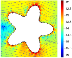
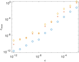
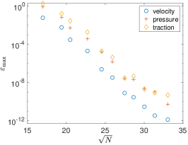
Figure 4: (a) Linear shear flow past a starfish-shaped island. Streamlines of the flow and panel endpoints (small segments) are shown. Color represents the $\log_{10}$ error of the velocity computed under tolerance $\epsilon=10^{-12}$ (resulted in $2N=2184$ degrees of freedom). (b) Convergence of the maximum relative error $\varepsilon_{\mathrm{max}}$ versus requested tolerance $\epsilon$, where the traction field is computed along the $(1,2)$-direction. (c) Convergence of the maximum error $\varepsilon_{\mathrm{max}}$ versus the square root of the number of nodes.

Example 2. Domain with corners.

The smooth geometry in Example 1 is now replaced with a non-convex polygon. Figure 5 shows a linear shear flow around a “shuriken” domain with eight corners, the outer four of which are reentrant (with respect to $\Omega$) corners of angle $\theta=1.74\pi$. With $\alpha=0.5$ for the flatter corners and $\alpha=1.1$ for the sharper ones, our scheme achieved accuracies that are matching the requested tolerance (Figure 5b). Note that the convergence with respect to problem size is super-algebraic (Figure 5c), and consistent with root-exponential convergence, as expected for problems with corner singularities (see Remark 4). We used the numerical solution obtained using $\epsilon=10^{-10}$ as the reference solution.

(a)	(b)	(c)

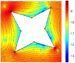
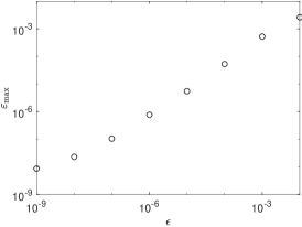
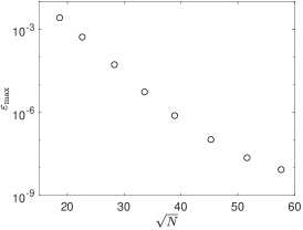
Figure 5: (a) Linear shear flow around a shuriken-shaped island with 8 corners. Streamlines of the flow and panel endpoints (small segments) are shown. Color represents the $\log_{10}$ error of the velocity computed under tolerance $\epsilon=10^{-10}$ (resulted in $2N=6640$ degrees of freedom). (b) Convergence of the maximum error $\varepsilon_{\mathrm{max}}$ versus requested tolerance $\epsilon$. (c) Convergence of the maximum error $\varepsilon_{\mathrm{max}}$ versus the square root of the number of nodes; root-exponential convergence would result in a straight line.

Example 3. Multiple polygonal islands.

This example models a porous media flow through a collection of non-smooth, non-convex and closely packed boundaries: we set up $50$ polygonal islands with a total number of 253 corners (Figure 6). The computational domain has width $\approx 8$ and the closest distance between the polygons is about $10^{-2}$. The background flow is the same as in the previous examples. With $\alpha=0.75$ and $\lambda=2$ for all corners, the convergence (Figure 6c) is similar to the single-polygon island example (Figure 5b–c), achieving more than 8 digits using approximately $800$ degrees of freedom per corner. This demonstrates the robustness of our adaptive scheme, that is, the performance is as good for a more complex example as for a simple one.

(a)	(b)	(c)

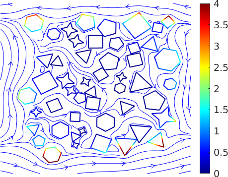
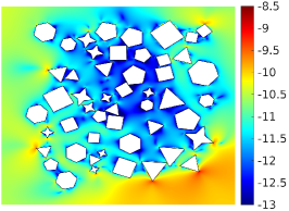
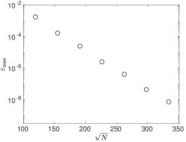
Figure 6: (a) Streamlines of a shear flow past $50$ randomly generated polygonal islands with a total number of 253 corners. Color on the polygon boundaries indicate the magnitude of density $\sigma$. (b) $\log_{10}$ of absolute error of the velocity, computed using $2N=222140$ degrees of freedom. Error is measured on a $1000\times 1000$ grid (spacing $\Delta x\approx 8.3\times 10^{-3}$) by comparing to the solution obtained with $\epsilon=10^{-10}$. (c) Convergence of the maximum error $\varepsilon_{\mathrm{max}}$ versus the square root of the number of nodes.

Example 4. Artificial vascular network.

We now turn to the example shown in Figure 2. We construct an artificial vascular network (with 378 corners) that mimics those observed in an eye of a zebra fish [53]. The flow in this network is driven by a uniform influx from the circular wall at the center and a uniform outflux at the outer circular wall, such that the overall volume is conserved; all other boundaries have a no-slip condition. We solve the BIE for this problem using GMRES with a block diagonal preconditioner consisting of the diagonal panel-wise blocks of the BIE system itself (i.e., the self-evaluation blocks for each panel). The FMM is used for applying the matrix and for final flow evaluations; see Remark 1. The sparse correction matrix (see Section 3.2) is applied via MATLAB’s single-threaded built-in matrix-vector multiplication; its rows have been precomputed as described in Section 3.4. All computations are done on an $8$-core $4.0$ GHz Intel Core i7 desktop.

Table 1 shows, for various tolerance $\epsilon$, the relative $L_{2}$-error $\varepsilon_{L_{2}}$, the relative maximum error in velocity $\varepsilon_{\mathrm{max}}$, the total number of panels used $n_{\Lambda}$, the number of degrees of freedom $2N$, memory (RAM) usage, the number of GMRES iterations and time used, the setup time for precomputing the close-correction matrices, and the percentage time for applying Stokes FMM during GMRES. Several observations are in order:

1. Both $\varepsilon_{L_{2}}$ and $\varepsilon_{\mathrm{max}}$ decay super-algebraically with the number of degrees of freedom; this data is plotted in Figure 7a. The closeness between $\varepsilon_{L_{2}}$ and $\varepsilon_{\mathrm{max}}$ shows that our scheme has achieved high accuracies near the sharper reentrant corners (hard) that are similar to those near the smooth edges (easy). This error analysis remains valid even in the zoomed-in high-resolution error plots in Figure 2. Furthermore, the convergence performance of this example is the same as the previous two examples—we achieved more than 8 digits, with a ratio $\frac{\text{degrees of freedom}}{\text{\#corners}}\approx 943$, which is similar to the ratios in Example 2 (830) and Example 3 (878). This once again demonstrates the robustness of our overall scheme to problem complexity.

2. The number of GMRES iterations increases only because we have requested smaller tolerance. Each additional digit needs about $100$ more iterations. The GMRES convergence rate is stable, which demonstrates that our second kind BIE formulation is well-conditioned even in the presence of corners.

3. The fact that the Stokes FMM time is the main cost shows that our algorithm has achieved close to optimal efficiency. The slight decrease of the percentage FMM times at smaller $\epsilon$ is due to the fact that the FMM time grows only linearly with $N$, while the close evaluation matrix-vector multiplication time grows like $O(N^{3/2})$. The latter estimate is obtained as follows. The number of matrix-vector multiplications grows like $O(n_{\Lambda})=O(\log 1/\epsilon)=O(p)$, where each matrix-vector product takes $O(p^{2})$ time. Note that $N=n_{\Lambda}\times p=O(p^{2})$, so the total close evaluation time grows as $O(p^{3})=O(N^{3/2})$. (See Figure 7b–d.)

$\epsilon$	$\varepsilon_{L_{2}}$	$\varepsilon_{\mathrm{max}}$	$n_{\Lambda}$	$2N$	RAM used(gb)	GMRES iteration	GMRES time(s)	setup time(s)	% FMM
1e-03	4.34e-04	5.43e-03	6549	52392	2.3	796	248	48	78.50
1e-04	2.20e-05	4.58e-04	8281	82810	2.9	919	458	63	77.86
1e-05	3.55e-06	7.21e-05	10301	123612	3.7	1091	759	84	75.92
1e-06	1.26e-06	7.15e-06	12061	168854	5.0	1282	1197	106	72.69
1e-07	2.53e-07	1.51e-06	14079	225264	6.9	1390	1670	135	70.91
1e-08	6.01e-09	1.58e-07	15839	285102	9.0	1501	2433	164	68.77
1e-09	1.44e-09	5.34e-08	17829	356580	12	1597	3195	204	66.16

Table 1: Results and statistics of solving the BVP in the vascular network in Figure 2 for various tolerance $\epsilon$. Errors $\varepsilon_{\mathrm{max}}$ and $\varepsilon_{L_{2}}$ are measured on a $2160\times 2160$ grid (spacing $\approx 2.5\times 10^{-3}$) by comparing to the solution obtained at $\epsilon=10^{-10}$. CPU time and RAM used are measured using [54].

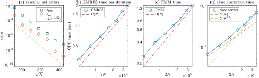
Figure 7: Error and timing of solving the vascular network BVP. (a) Convergence of errors in log-linear scale. (b) Log-log scale plot of the total CPU time per GMRES iteration, which consists of the FMM time, shown in (c), and the close correction time, shown in (d).

Example 5. Uniform versus adaptive for close-to-touching curves.

Finally, to demonstrate the advantage of using an adaptive scheme over a uniform discretization, let us consider a uniform flow past two close-to-touching disks (Figure 8). The background flow is a constant $u_{\infty}=(1,0)$, the separation is $d=10^{-6}$, and the radii 1 and 0.1. For the uniform-resolution scheme we use a global periodic trapezoid grid on each circle, where, in order to have similar node spacings, the larger circle has $9$ times as many points as the smaller one. Here, global close-evaluation is done using the spectrally accurate quadrature from [25]. On the other hand, the adaptive quadrature uses a grid that is determined by our adaptive refinement scheme of Section 4, with one modification that improves the scaling in the number of refined panels (see Remark 5). We observe that, for more than 4 accurate digits, the number of unknowns required by the adaptive scheme is much less than that of the uniform-resolution scheme (Figure 8). The smoothness of the density function discussed in the remark below suggests that, at fixed $\epsilon$, the uniform scheme (and also the original refinement scheme) needs $N=O(1/\sqrt{d})$ unknowns, whereas the modified adaptive scheme needs only $N=O(\log(1/d))$. The latter is close to optimal, and is what we recommend for closely-interacting curves. (See also Examples 4 and 6 in [55] for a “globally adaptive” variant.)

Remark 5 (Refinement at close-to-touching smooth surfaces).

For viscous flow in the region between two smooth curves separated by a small distance $d$, asymptotic analysis gives that the width of the “bump” in fluid force scales as $O(\sqrt{d})$ [56]. By dimensional analysis, if the sum of the two curvatures of the surfaces near the contact point is $\kappa$, then the width in fact scales as $O(\sqrt{d/\kappa})$. Assuming that this also applies to the density $\sigma$, this suggests a looser criterion for refinement: panels should be refined only when they are longer than this width scale. This allows panels to come much closer than their length, without being refined. In the case of close smooth curves, the test in line 13 of Algorithm 2 can thus be modified to $(c^{\prime}\sqrt{\kappa}S)^{2}>d$. We find that the constant $c^{\prime}=0.7$ achieves the requested tolerance. The resulting $N$ can be estimated as follows. Setting $\kappa=1$ for simplicity, a generic local model of the separation is $h(t)\approx d+t^{2}$ as a function of parameter $t$, and $n_{\Lambda}=O\bigl{(}\int_{-1}^{1}dt/S(h(t))\,\bigr{)}$ where $S(h)$ is the local panel size as a function of separation. The original refinement scheme, $S(h)=O(h)$, thus gives $n_{\Lambda}=O(d^{-1/2})$, whereas the modified $S(h)=O(\sqrt{h})$ gives $n_{\Lambda}=O(\log(1/d))$.

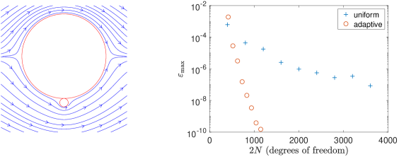
Figure 8: Convergence of a uniform flow past two touching disks that are $d=10^{-6}$ apart, and whose radii are 1 and 0.1. The required number of unknowns in the adaptive scheme is much less than the global scheme with uniform resolution; see Example 5.

6 Conclusions

We have presented a set of panel quadrature rules for accurate evaluation of single- and double-layer Stokes potentials and their associated pressure and traction boundary integrals. They can be used for targets that are either on or off the boundary, and can be located arbitrarily close to it. In addition, we formulated an adaptive panel refinement procedure that sets the length of panels on the boundary (“$h$-adaptivity”) and the overall degree of approximation $p$ (“$p$-adaptivity”) required to achieve a user-prescribed tolerance. We demonstrated via numerical experiments that our algorithm achieves super-algebraic convergence even for complex geometries with corners, and that the CPU time grows linearly with problem size, and is dominated by the cost of FMMs for large-scale problems. More sophisticated quadratures and techniques designed for corner singularities, such as the RCIP [57, 58] (or the work of [39]), are expected to further improve the performance of our BIE solver. It is also expected that adapting $p$ on a per-panel basis (i.e. full $hp$-adaptivity) would reduce the total number of degrees of freedom needed, although only by a factor less than two. Applications of our work include providing design tools for rapid prototyping of microfluidic chips (for cell sorting, mixing or other manipulations e.g., [59]), shape optimization (e.g., [60]) and simulating cellular-level blood flow in microvasculature.

We envision building a fast 2D particulate flow software library by utilizing the algorithms developed in this work for the fixed complex geometries (such as microfluidic chips or vascular networks) and our global close evaluation schemes developed in [25] for the moving rigid or deformable particles (such as colloids, drops or vesicles). Another key ingredient would be a fast direct solver for solving the BIEs on the fixed geometries, similar to that developed in [61], wherein the boundary integral operators were compressed by exploiting their low-rank structures, inverted as a precomputation step, and applied at an optimal $O(N)$ cost at every time-step of the particulate flow simulation as particles move through the fixed geometry. One open research question in this context is: Can we update the compressed representations as the boundary panels are refined (or coarsened) without rebuilding them? A similar question was recently investigated in [62], where the authors report a $3\times$ speedup when locally perturbing the geometry. We plan to explore their approach and report its performance in the context of our adaptive panel refinement procedure.

7 Acknowledgements

We thank Leslie Greengard and Manas Rachh for many useful discussions pertaining to this work. We thank Manas Rachh for his biharmonic FMM code, and Jun Wang for providing Stokes MATLAB wrappers to this code. We acknowledge support from NSF under grants DMS-1719834 and DMS-1454010. The work of SV was also supported by the Flatiron Institute, a division of the Simons Foundation.

Appendix A Pressure and traction in terms of contour integrals

Here, we give formulae for the traction vector $\bf T$ induced at a target point with given surface normal, and the associated pressure field $p$, when the velocity field is represented by a Stokes single or double layer potential. The goal is to write the traction and pressure in terms of the four contour integrals of Sec. 2.2, to which close-evaluation methods of Sec. 3.3 may then be applied. This enables uniformly accurate force calculations on bodies, or solution of traction BVPs. We use the notation of Sec. 2: recall that $r=x-y$, $n_{x}$ and $n_{y}$ are the normal vectors at the target $x$ and source $y$ respectively, $\rho=|r|$, and $I$ denotes the $2\times 2$ identity operator.

We first consider the single layer potential (3). Its traction is

$$(\mathbf{T}^{S}\sigma)(x)=-\dfrac{1}{\pi}\int_{\Gamma}\dfrac{r\cdot n_{x}}{\rho^{2}}\,\dfrac{r\otimes r}{\rho^{2}}\sigma(y)\,ds_{y},$$ (47)

which turns out to be the negative of the Stokes DLP (4) with $n_{y}$ replaced by $n_{x}$. While (17) is no longer useful in this case, we can instead write the traction as

$$(\mathbf{T}^{S}\sigma)(x)=-\dfrac{1}{\pi}\int_{\Gamma}(r\cdot\sigma(y))\dfrac{r}{\rho^{4}}(r\cdot n_{x})\,ds_{y}$$ (48)

and use the slightly different identity

$$\nabla_{x}\left(\dfrac{r\cdot\sigma}{\rho^{2}}\right)=\dfrac{\sigma}{\rho^{2}}-(r\cdot\sigma)\dfrac{2r}{\rho^{4}}$$ (49)

to write the traction kernel as

$$(\mathbf{T}^{S}\sigma)(x)\;= {-1\over 2\pi}\int_{\Gamma}{r\cdot n_{x}\over\rho^{2}}\sigma\,ds_{y}+{1\over 2\pi}(x\cdot n_{x})\nabla\int_{\Gamma}{r\cdot\sigma\over\rho^{2}}\,ds_{y}$$ (50)

$$-{1\over 2\pi}n_{x,1}\nabla\int_{\Gamma}{r\cdot\sigma\over\rho^{2}}y_{1}\,ds_{y}-{1\over 2\pi}n_{x,2}\nabla\int_{\Gamma}{r\cdot\sigma\over\rho^{2}}y_{2}\,ds_{y}\leavevmode\nobreak\ ,$$

where $(n_{x,1},n_{x,2})=:n_{x}$ are the two components of $n_{x}$. As did in the case of velocity potentials, we can concisely write (50) as

$$\mathbf{T}^{S}\sigma=\big{(}(\mathcal{S}\sigma_{1})_{n}+i(\mathcal{S}\sigma_{2})_{n}\big{)}+\frac{1}{2\pi}\left(\text{Re}(x/n_{x})\overline{I_{H}(\sigma/n_{y})}-n_{x,1}\overline{I_{H}(\sigma y_{1}/n_{y})}-n_{x,2}\overline{I_{H}(\sigma y_{2}/n_{y})}\right),$$ (51)

where all the $\mathbb{R}^{2}$ vectors are now understood as complex numbers in $\mathbb{C}$, the over line in $\overline{I_{H}(\cdot)}$ denotes the complex conjugate of $I_{H}(\cdot)$ and the dot product $x\cdot n_{x}=\text{Re}(x/n_{x})$ is due to the fact that $1=|n_{x}|^{2}=n_{x}\overline{n_{x}}$.

The single layer pressure associated to (3) is

$$(P^{S}\sigma)(x)=\dfrac{1}{2\pi}\int_{\Gamma}\dfrac{r\cdot\sigma}{\rho^{2}}\,ds_{y}\leavevmode\nobreak\ ,$$ (52)

which again in the complex plane can be written as

$$P^{S}\sigma=\text{Re}\frac{i}{2\pi}I_{C}(\sigma/n_{y}).$$ (53)

We now turn to the Stokes double layer potential (4). The traction kernel and its associated pressure kernel are given by [63, (5.27)] [55, (3.37)],

$$(\mathbf{T}^{D}\sigma)(x)= \frac{\mu}{\pi}\int_{\Gamma}\left(-8\frac{r\otimes r}{\rho^{6}}(r\cdot n_{x})(r\cdot n_{y})+\frac{r\otimes n_{x}}{\rho^{4}}(r\cdot n_{y})+\frac{r\otimes r}{\rho^{4}}(n_{x}\cdot n_{y})\right.$$ (54)

$$\left.\hskip 65.04256pt+I\frac{1}{\rho^{4}}(r\cdot n_{x})(r\cdot n_{y})+\frac{n_{y}\otimes r}{\rho^{4}}(r\cdot n_{x})+\frac{n_{x}\otimes n_{y}}{\rho^{2}}\right)\sigma(y)\,ds_{y}$$

$$(P^{D}\sigma)(x)= \frac{\mu}{\pi}\int_{\Gamma}\left(-\frac{n_{y}\cdot\sigma(y)}{\rho^{2}}+2\frac{r\cdot\sigma(y)}{\rho^{4}}\left(r\cdot n_{y}\right)\right)\,ds_{y}.$$

The corresponding boundary integral operators $(\mathbf{T}^{D}\sigma)(x)$ and $(P^{D}\sigma)(x)$ are hyper-singular. We can easily derive the following equation expressing this operator in terms of the Laplace double layer potential:

$$\frac{1}{\mu}\mathbf{T}^{D}\sigma= -2\left(x\cdot n_{x}\nabla\nabla\mathcal{D}[\sigma]-n_{x,1}\nabla\nabla\mathcal{D}[y_{1}\sigma]-n_{x,2}\nabla\nabla[y_{2}\sigma]\right)$$ (55)

$$+3I(n_{x}\cdot\nabla\mathcal{D})[\sigma]-(n_{x}\otimes\nabla\mathcal{D})[\sigma]-(\nabla\mathcal{D}\otimes n_{x})[\sigma]$$

$$+\begin{bmatrix}1&\\ &-1\end{bmatrix}\left(n_{x}\cdot\nabla\mathcal{D}+n_{x}\otimes\nabla\mathcal{D}-\nabla\mathcal{D}\otimes n_{x}\right)\left[\frac{\bar{n}_{y}}{n_{y}}\sigma\right],$$

$$P^{D}\sigma= -2\mu\left(\frac{\partial}{\partial x_{1}}\mathcal{D}[\sigma_{1}]+\frac{\partial}{\partial x_{2}}\mathcal{D}[\sigma_{2}]\right)$$

$$= \frac{\mu}{\pi}\left(\text{Im}\left(I_{H}(\sigma_{1})\right)+\text{Re}\left(I_{H}(\sigma_{2})\right)\right).$$

Here $\frac{\bar{n}_{y}}{n_{y}}\sigma=[\frac{\bar{n}_{y}}{n_{y}}\sigma_{1},\frac{\bar{n}_{y}}{n_{y}}\sigma_{2}]^{T}$, $\nabla$ is short for $\nabla_{x}$, and $\nabla\nabla$ is the Hessian tensor. The gradients of Laplace double-layer potentials needed above are expressed in terms of Hadamard integrals using (15). The Hessians are given in terms of supersingular integrals as follows:

$$\nabla\nabla\mathcal{D}[\sigma](x)\;=\;\begin{bmatrix}\text{Re}\frac{i}{\pi}\left(I_{S}(\sigma_{1})\right)(x)&-\text{Im}\frac{i}{\pi}\left(I_{S}(\sigma_{2})\right)(x)\\ -\text{Im}\frac{i}{\pi}\left(I_{S}(\sigma_{1})\right)(x)&-\text{Re}\frac{i}{\pi}\left(I_{S}(\sigma_{2})\right)(x)\end{bmatrix}.$$ (56)

The close evaluation formulae for these are in Sec. 3.3.3.

To validate the above formulae, we include in Fig. 4(b–c) the convergence of the maximum error in pressure and traction for the smooth domain of Example 1 from Sec. 5. The convergence rate is very similar to that of velocity albeit a loss of 1–2 digits, which is expected due to the extra derivatives.

References

- [1] Youngren G. K. and A. Acrivos. Stokes flow past a particle of arbitrary shape: a numerical method of solution. Journal of Fluid Mechanics, 69:377–403, May 1975.
- [2] Youngren G. K. and A. Acrivos. On the shape of a gas bubble in a viscous extensional flow. Journal of Fluid Mechanics, 76:433–442, August 1976.
- [3] Chiara Sorgentone and Anna-Karin Tornberg. A highly accurate boundary integral equation method for surfactant-laden drops in 3D. Journal of Computational Physics, 360:167–191, 2018.
- [4] Abtin Rahimian, Shravan K Veerapaneni, Denis Zorin, and George Biros. Boundary integral method for the flow of vesicles with viscosity contrast in three dimensions. Journal of Computational Physics, 298:766–786, 2015.
- [5] Spencer H Bryngelson and Jonathan B Freund. Global stability of flowing red blood cell trains. Physical Review Fluids, 3(7):073101, 2018.
- [6] Leslie Greengard, Mary Catherine Kropinski, and Anita Mayo. Integral equation methods for Stokes flow and isotropic elasticity in the plane. Journal of Computational Physics, 125(2):403–414, 1996.
- [7] L. Ying, G. Biros, and D. Zorin. A kernel-independent adaptive fast multipole method in two and three dimensions. Journal of Computational Physics, 196(2):591–626, 2004.
- [8] Haitao Wang, Ting Lei, Jin Li, Jingfang Huang, and Zhenhan Yao. A parallel fast multipole accelerated integral equation scheme for 3D Stokes equations. International journal for numerical methods in engineering, 70(7):812–839, 2007.
- [9] Anna-Karin Tornberg and Leslie Greengard. A fast multipole method for the three-dimensional Stokes equations. Journal of Computational Physics, 227(3):1613–1619, 2008.
- [10] Zydrunas Gimbutas and Leslie Greengard. Computational software: Simple FMM libraries for electrostatics, slow viscous flow, and frequency-domain wave propagation. Communications in Computational Physics, 18(2):516–528, 2015.
- [11] Dhairya Malhotra and George Biros. PVFMM: A parallel kernel independent FMM for particle and volume potentials. Communications in Computational Physics, 18(3):808–830, 2015.
- [12] David Saintillan, Eric Darve, and Eric SG Shaqfeh. A smooth particle-mesh Ewald algorithm for Stokes suspension simulations: The sedimentation of fibers. Physics of Fluids, 17(3):033301, 2005.
- [13] Dag Lindbo and Anna-Karin Tornberg. Spectrally accurate fast summation for periodic Stokes potentials. Journal of Computational Physics, 229(23):8994–9010, 2010.
- [14] Amit Kumar and Michael D Graham. Accelerated boundary integral method for multiphase flow in non-periodic geometries. Journal of Computational Physics, 231(20):6682–6713, 2012.
- [15] Ludvig af Klinteberg, Davoud Saffar Shamshirgar, and Anna-Karin Tornberg. Fast Ewald summation for free-space Stokes potentials. Research in the Mathematical Sciences, 4(1):1, 2017.
- [16] Ashok S Sangani and Guobiao Mo. An algorithm for Stokes and Laplace interactions of particles. Physics of Fluids, 8(8):1990–2010, 1996.
- [17] A.Z. Zinchenko and R.H. Davis. An efficient algorithm for hydrodynamical interaction of many deformable drops. Journal of Computational Physics, 157(2):539–587, 2000.
- [18] Xin Wang, Joe Kanapka, Wenjing Ye, Narayan R Aluru, and Jacob White. Algorithms in FastStokes and its application to micromachined device simulation. IEEE Transactions on computer-aided design of integrated circuits and systems, 25(2):248–257, 2006.
- [19] Lei Wang, Svetlana Tlupova, and Robert Krasny. A treecode algorithm for 3D stokeslets and stresslets. arXiv preprint arXiv:1811.12498, 2018.
- [20] Abtin Rahimian, Ilya Lashuk, Shravan Veerapaneni, Aparna Chandramowlishwaran, Dhairya Malhotra, Logan Moon, Rahul Sampath, Aashay Shringarpure, Jeffrey Vetter, Richard Vuduc, Denis Zorin, and George Biros. Petascale direct numerical simulation of blood flow on 200k cores and heterogeneous architectures. In Proceedings of the 2010 ACM/IEEE International Conference for High Performance Computing, Networking, Storage and Analysis, SC ’10, pages 1–11, 2010.
- [21] Ehssan Nazockdast, Abtin Rahimian, Denis Zorin, and Michael Shelley. A fast platform for simulating semi-flexible fiber suspensions applied to cell mechanics. Journal of Computational Physics, 329:173–209, 2017.
- [22] Wen Yan, Eduardo Corona, Dhairya Malhotra, Shravan Veerapaneni, and Michael Shelley. A scalable computational platform for particulate Stokes suspensions. under review, 2019.
- [23] S Elizabeth Hulme, Sergey S Shevkoplyas, Javier Apfeld, Walter Fontana, and George M Whitesides. A microfabricated array of clamps for immobilizing and imaging c. elegans. Lab on a Chip, 7(11):1515–1523, 2007.
- [24] Takuji Ishikawa and TJ Pedley. The rheology of a semi-dilute suspension of swimming model micro-organisms. Journal of Fluid Mechanics, 588:399–435, 2007.
- [25] Alex Barnett, Bowei Wu, and Shravan Veerapaneni. Spectrally accurate quadratures for evaluation of layer potentials close to the boundary for the 2D Stokes and Laplace equations. SIAM Journal on Scientific Computing, 37(4):B519–B542, 2015.
- [26] Rikard Ojala and Anna-Karin Tornberg. An accurate integral equation method for simulating multi-phase Stokes flow. Journal of Computational Physics, 298:145–160, 2015.
- [27] J. Helsing and R. Ojala. On the evaluation of layer potentials close to their sources. Journal of Computational Physics, 227:2899–2921, 2008.
- [28] M. C. A. Kropinski. An efficient numerical method for studying interfacial motion in two-dimensional creeping flows. Journal of Computational Physics, 171(2):479–508, 2001.
- [29] Andreas Klöckner, Alexander Barnett, Leslie Greengard, and Michael O’Neil. Quadrature by expansion: A new method for the evaluation of layer potentials. Journal of Computational Physics, 252:332–349, 2013.
- [30] Alex H Barnett. Evaluation of layer potentials close to the boundary for Laplace and Helmholtz problems on analytic planar domains. SIAM Journal on Scientific Computing, 36(2):A427–A451, 2014.
- [31] Camille Carvalho, Shilpa Khatri, and Arnold D Kim. Asymptotic analysis for close evaluation of layer potentials. Journal of Computational Physics, 355:327–341, 2018.
- [32] Abtin Rahimian, Alex Barnett, and Denis Zorin. Ubiquitous evaluation of layer potentials using quadrature by kernel-independent expansion. BIT Numerical Mathematics, 58(2):423–456, 2018.
- [33] Ludvig af Klinteberg and Anna-Karin Tornberg. Adaptive quadrature by expansion for layer potential evaluation in two dimensions. arXiv preprint arXiv:1704.02219, 2017.
- [34] Carlos Pérez-Arancibia, Luiz M Faria, and Catalin Turc. Harmonic density interpolation methods for high-order evaluation of laplace layer potentials in 2D and 3D. Journal of Computational Physics, 376:411–434, 2019.
- [35] Shravan K. Veerapaneni, Abtin Rahimian, George Biros, and Denis Zorin. A fast algorithm for simulating vesicle flows in three dimensions. J. Comput. Phys., 230(14):5610–5634, 2011.
- [36] Eisuke Kita and Norio Kamiya. Error estimation and adaptive mesh refinement in boundary element method, an overview. Engineering Analysis with Boundary Elements, 25(7):479–495, 2001.
- [37] N Heuer and E P Stephan. The -version of the boundary element method on polygons. J. Integral Equ. Appl., 8(2):173–212, 1996.
- [38] Markus Bantle and Stefan Funken. Efficient and accurate implementation of -BEM for the Laplace operator in 2D. Applied Numerical Mathematics, 95:51 – 61, 2015. Fourth Chilean Workshop on Numerical Analysis of Partial Differential Equations (WONAPDE 2013).
- [39] Manas Rachh and Kirill Serkh. On the solution of Stokes equation on regions with corners. arXiv preprint arXiv:1711.04072; submitted to Comm. Pure Appl. Math., 2017.
- [40] Constantine Pozrikidis. Boundary integral and singularity methods for linearized viscous flow. Cambridge University Press, 1992.
- [41] G. C. Hsiao and W. L. Wendland. Boundary integral equations, volume 164 of Applied Mathematical Sciences. Springer, 2008.
- [42] F.-K. Hebeker. Efficient boundary element methods for three-dimensional exterior viscous flows. Numer. Methods Partial Differential Equations, 2:273–297, 1986.
- [43] Rainer Kress. Linear Integral Equations, volume 82 of Applied Mathematical Sciences. Springer, 2nd edition, 1999.
- [44] M Rachh. bhfmm2d: parallel Fortran code for the biharmonic FMM in 2D, 2012.
- [45] A Greenbaum, L Greengard, and A Mayo. On the numerical solution of the biharmonic equation in the plane. Physica D, 60(1–4):216–225, 1992.
- [46] S. Hao, A. H. Barnett, P. G. Martinsson, and P. Young. High-order accurate Nyström discretization of integral equations with weakly singular kernels on smooth curves in the plane. Adv. Comput. Math., 40(1):245–272, 2014.
- [47] Lloyd N Trefethen. Approximation theory and approximation practice, volume 128. SIAM, 2013.
- [48] L af Klinteberg and A-K Tornberg. Adaptive quadrature by expansion for layer potential evaluation in two dimensions. SIAM J. Sci. Comput., 40(3):A1225—A1249, 2018.
- [49] V Y Pan. How bad are Vandermonde matrices? SIAM J. Matrix Anal. Appl., 37(2):676–694, 2016.
- [50] S S Zargaryan and V G Maz’ya. The asymptotic form of the solutions of the integral equations of potential theory in the neighbourhood of the corner points of a contour. Prikl. Matem. Mekhan. U.S.S.R., 48(1):120–124, 1984.
- [51] Andrea Tagliasacchi. kdtree code. https://www.mathworks.com/matlabcentral/fileexchange/21512-ataiya-kdtree, 2017.
- [52] Abinand Gopal and Lloyd N. Trefethen. Solving Laplace problems with corner singularities via rational functions. SIAM Journal on Numerical Analysis (to appear), 2019.
- [53] Yolanda Alvarez, Maria L Cederlund, David C Cottell, Brent R Bill, Stephen C Ekker, Jesus Torres-Vazquez, Brant M Weinstein, David R Hyde, Thomas S Vihtelic, and Breandan N Kennedy. Genetic determinants of hyaloid and retinal vasculature in zebrafish. BMC developmental biology, 7(1):114, 2007.
- [54] Alex Barnett. memorygraph: a MATLAB/octave unix tool to record true memory and CPU usage vs time. https://github.com/ahbarnett/memorygraph, 2018.
- [55] Alex H Barnett, Gary R Marple, Shravan Veerapaneni, and Lin Zhao. A unified integral equation scheme for doubly periodic Laplace and Stokes boundary value problems in two dimensions. Communications on Pure and Applied Mathematics, 71(11):2334–2380, 2018.
- [56] Ashok S Sangani and Guobiao Mo. Inclusion of lubrication forces in dynamic simulations. Physics of fluids, 6(5):1653–1662, 1994.
- [57] Johan Helsing. Solving integral equations on piecewise smooth boundaries using the rcip method: a tutorial. In Abstract and Applied Analysis, volume 2013. Hindawi, 2013.
- [58] Johan Helsing and Shidong Jiang. On integral equation methods for the first Dirichlet problem of the biharmonic and modified biharmonic equations in nonsmooth domains. SIAM Journal on Scientific Computing, 40(4):A2609–A2630, 2018.
- [59] Gökberk Kabacaoğlu and George Biros. Optimal design of deterministic lateral displacement device for viscosity-contrast-based cell sorting. Physical Review Fluids, 3(12):124201, 2018.
- [60] Marc Bonnet, Ruowen Liu, and Shravan Veerapaneni. Shape optimization of Stokesian peristaltic pumps using boundary integral methods. arXiv preprint arXiv:1903.03634, 2019.
- [61] Gary Marple, Alexander H. Barnett, Adrianna Gillman, and Shravan K. Veerapaneni. A fast algorithm for simulating multiphase flows through periodic geometries of arbitrary shape. SIAM Journal on Scientific Computing, 38(5):B740–B772, 2016.
- [62] Yabin Zhang and Adrianna Gillman. A fast direct solver for boundary value problems on locally perturbed geometries. Journal of Computational Physics, 356:356–371, 2018.
- [63] Y Liu. Fast Multipole Boundary Element Method: Theory and Applications in Engineering. Cambridge University Press, 2009.