Maximum Amplification of Enstrophy in 3D Navier-Stokes Flows

Abstract

This investigation concerns a systematic search for potentially singular behavior in 3D Navier-Stokes flows. Enstrophy serves as a convenient indicator of the regularity of solutions to the Navier Stokes system — as long as this quantity remains finite, the solutions are guaranteed to be smooth and satisfy the equations in the classical (pointwise) sense. However, there are no estimates available with finite a priori bounds on the growth of enstrophy and hence the regularity problem for the 3D Navier-Stokes system remains open. In order to quantify the maximum possible growth of enstrophy, we consider a family of PDE optimization problems in which initial conditions with prescribed enstrophy ${\mathcal{E}}_{0}$ are sought such that the enstrophy in the resulting Navier-Stokes flow is maximized at some time $T$. Such problems are solved computationally using a large-scale adjoint-based gradient approach derived in the continuous setting. By solving these problems for a broad range of values of ${\mathcal{E}}_{0}$ and $T$, we demonstrate that the maximum growth of enstrophy is in fact finite and scales in proportion to ${\mathcal{E}}_{0}^{3/2}$ as ${\mathcal{E}}_{0}$ becomes large. Thus, in such worst-case scenario the enstrophy still remains bounded for all times and there is no evidence for formation of singularity in finite time. We also analyze properties of the Navier-Stokes flows leading to the extreme enstrophy values and show that this behavior is realized by a series of vortex reconnection events.

1 Introduction

The goal of this study is to assess the largest growth of enstrophy possible in finite time in viscous incompressible flows in three dimensions (3D). This problem is motivated by the question whether solutions to the 3D incompressible Navier-Stokes system on unbounded or periodic domains corresponding to smooth initial data may develop a singularity in finite time (Doering, 2009). By formation of a “singularity” we mean the situation when some norms of the solution starting from smooth initial data become unbounded after a finite time. This so-called “blow-up problem” is one of the key open questions in mathematical fluid mechanics and, in fact, its importance for mathematics in general has been recognized by the Clay Mathematics Institute as one of its “millennium problems” (Fefferman, 2000). Should such singular behavior indeed be possible in the solutions of the 3D Navier-Stokes problem, it would invalidate this system as a model of realistic fluid flows. Questions concerning global-in-time existence of smooth solutions remain open also for a number of other flow models including the 3D Euler equations (Gibbon et al., 2008) and some of the “active scalar” equations (Kiselev, 2010).

At the same time, it is known that suitably defined weak solutions, which need not satisfy the Navier-Stokes system pointwise in space and time, but rather in a certain integral sense only, exist globally in time (Leray, 1934). An important tool in the study of the global-in-time regularity of classical (smooth) solutions are the so-called “conditional regularity results” stating additional conditions which must be satisfied by a weak solution in order for it to also be a smooth solution, i.e., to satisfy the Navier-Stokes system in the classical sense as well. One of the best known results of this type, due to Foias & Temam (1989), is based on the enstrophy ${\mathcal{E}}$ (see below, cf. (5), for a precise definition of this quantity) of the time-dependent velocity field ${\mathbf{u}}(t)$ and asserts that if the uniform bound

$$\mathop{\sup}_{0\leq t\leq T}{\mathcal{E}}({\mathbf{u}}(t))<\infty$$ (1)

holds, then the regularity and uniqueness of the solution ${\mathbf{u}}(t)$ are guaranteed up to time $T$ (to be precise, the solution remains in a certain Gevrey class). Other well-known conditional regularity results are given by the Ladyzhenskaya-Prodi-Serrin conditions in which global-in-time regularity follows from certain integrability criteria imposed in space and in time on the velocity field ${\mathbf{u}}(t)$ (Kiselev & Ladyzhenskaya, 1957; Prodi, 1959; Serrin, 1962). These results were recently extended and generalized by Gibbon (2018) who derived analogous conditions applicable to derivatives of various degrees of the velocity field. We add that Tao (2016) recently showed that solutions to a certain suitably-averaged version of the Navier-Stokes equation may exhibit blow-up in finite time. One of the insights from this work is that understanding singular behavior in the Navier-Stokes flows will likely require more refined tools than the currently available techniques of harmonic analysis.

From the practical point of view, the advantage of using the conditional regularity result (1) is that the quantity it involves, the enstrophy ${\mathcal{E}}({\mathbf{u}}(t))$, is very convenient to work with, especially in the context of numerical optimization problems. More specifically, since the enstrophy is a seminorm on a Hilbert space, formulation of such optimization problems for the Navier-Stokes system, which are the main tool to be used in this study, is relatively straightforward. In addition, in being directly related to vorticity, the enstrophy is also physically meaningful. Condition (1) implies that, should singularity indeed form in finite time, then all Sobolev norms of order higher than or equal one of the solution must blow up simultaneously. In the context of the inviscid Euler system a conditional regularity result similar to (1) is given by the Beale-Kato-Majda (BKM) criterion (Beale et al., 1984). The goal of the present investigation is to probe condition (1) computationally by constructing flow evolutions designed to produce the largest possible increase of enstrophy in some prescribed time $T$. Such worst-case behavior will be determined systematically by solving a family of suitably defined variational optimization problems.

While the blow-up problem is fundamentally a question in mathematical analysis, a lot of computational studies have been carried out since the mid-’80s in order to shed light on the hydrodynamic mechanisms which might lead to singularity formation in finite time. Given that such flows evolving near the edge of regularity involve formation of very small flow structures, these computations typically require the use of state-of-the-art computational resources available at a given time. The computational studies focused on the possibility of finite-time blow-up in the 3D Navier-Stokes and/or Euler system include Brachet et al. (1983); Pumir & Siggia (1990); Brachet (1991); Kerr (1993); Pelz (2001); Bustamante & Kerr (2008); Ohkitani & Constantin (2008); Ohkitani (2008); Grafke et al. (2008); Gibbon et al. (2008); Hou (2009); Orlandi et al. (2012); Bustamante & Brachet (2012); Orlandi et al. (2014); Campolina & Mailybaev (2018), all of which considered problems defined on domains periodic in all three dimensions. The investigations by Donzis et al. (2013); Kerr (2013b); Gibbon et al. (2014); Kerr (2013a) focused on the time evolution of vorticity moments and compared it against bounds on these quantities obtained using rigorous analysis. Recent computations by Kerr (2018) considered a “trefoil” configuration meant to be defined on an unbounded domain (although the computational domain was always truncated to a finite periodic box). A simplified semi-analytic model of vortex reconnection was recently developed and analyzed based on the Biot-Savart law and asymptotic techniques by Moffatt & Kimura (2019a, b). We also mention the studies by Matsumoto et al. (2008) and Siegel & Caflisch (2009), along with references found therein, in which various complexified forms of the Euler equation were investigated. The idea of this approach is that, since the solutions to complexified equations have singularities in the complex plane, singularity formation in the real-valued problem is manifested by the collapse of the complex-plane singularities onto the real axis. Overall, the outcome of these investigations is rather inconclusive: while for the Navier-Stokes system most of the recent computations do not offer support for finite-time blow-up, the evidence appears split in the case of the Euler system. In particular, the studies by Bustamante & Brachet (2012) and Orlandi et al. (2012) hinted at the possibility of singularity formation in finite time. In this connection we also highlight the computational investigations by Luo & Hou (2014a, b) in which blow-up was documented in axisymmetric Euler flows on a bounded (tubular) domain. Recently, Elgindi & Jeong (2018) proved finite-time singularity formation in 3D axisymmetric Euler flows on domains exterior to a boundary with conical shape.

A common feature of all of the aforementioned investigations was that the initial data for the Navier-Stokes or Euler system was chosen in an ad-hoc manner, based on some heuristic arguments. On the other hand, in the present study we pursue a fundamentally different approach, proposed originally by Lu & Doering (2008) and employed also by Ayala & Protas (2011, 2014a, 2014b, 2017); Yun & Protas (2018) for a range of related problems, in which the initial data leading to the most singular behaviour is sought systematically via solution of a suitable variational optimization problem. In the present investigation we look for the initial data which, subject to some constraints, will lead to flow evolution maximizing the enstrophy growth over some prescribed time interval $[0,T]$, where $0<T<\infty$, with the intention of verifying whether this growth could possibly become unbounded. Since the flow evolution is governed by the Navier-Stokes system of partial differential equations (PDEs), this leads to a PDE-constrained optimization problem for the initial data ${\mathbf{u}}_{0}$ which is amenable to solution using a gradient approach with gradient information obtained from the solutions of an adjoint system. The motivation for this investigation comes from our earlier study (Ayala & Protas, 2017), see also Lu & Doering (2008), where families of vortex states maximizing the instantaneous rate of growth of enstrophy were found. Although these vector fields did saturate the rigorous upper bounds on the instantaneous rate of growth of enstrophy, this maximal growth was in fact very rapidly depleted during the subsequent flow evolution, resulting in a very small only increase of enstrophy over finite times. The main conclusion from this result is that if an unbounded growth of enstrophy should be possible under the 3D Navier-Stokes dynamics, it must be associated with “instantaneously suboptimal” initial data which does not maximize the instantaneous rate of enstrophy production. In the present investigation we embark on a systematic search for such initial data.

It ought to be emphasized that solution of optimization problems involving the 3D time-dependent Navier-Stokes system leads to very challenging computational problems even at moderate Reynolds numbers. We remark that, in order to establish a direct link with the results of the mathematical analysis discussed below, in our investigation we therefore follow a rather different strategy than in most of the computational studies of extreme Navier-Stokes and Euler flows referenced above. While these earlier studies relied on data from a relatively small number of simulations performed at a high (at the given time) resolution, in the present investigation we explore a broad range of cases, each of which is however computed at a more moderate resolution (or, equivalently, Reynolds number). With such an approach to the use of available computational resources, we are able to reveal trends resulting from the variation of key parameters which otherwise would be hard to detect. Systematic computations conducted in this way thus allow us to establish sharpness of various a priori estimates relevant for a given problem; if these estimates turn out not to be sharp, or are not available, then such results can help formulate “targets” for what can potentially be proved.

By addressing the question about the maximum growth of enstrophy possible in finite time in the 3D Navier-Stokes system, the present investigation represents an important milestone in our long-term research program in which analogous questions have also been considered in the context of more tractable problems involving the one-dimensional (1D) Burgers equation and the two-dimensional (2D) Navier-Stokes system. Although global-in-time existence of classical (smooth) solutions is well known for both these problems (Kreiss & Lorenz, 2004), questions concerning the sharpness of the corresponding estimates for the instantaneous and finite-time growth of various enstrophy-like quantities are relevant, because these estimates are obtained using essentially the same methods as employed to derive their 3D counterparts. Since in 2D flows on unbounded or periodic domains the enstrophy may not increase ($d{\mathcal{E}}/dt\leq 0$), the relevant quantity in this case is the palinstrophy ${\mathcal{P}}({\mathbf{u}}(t)):=\frac{1}{2}\int_{\Omega}|\boldsymbol{\nabla}\boldsymbol{\omega}(t,{\mathbf{x}})|^{2}\,d{\mathbf{x}}$, where $\boldsymbol{\omega}:=\boldsymbol{\nabla}\times{\mathbf{u}}$ is the vorticity (which reduces to a pseudo-scalar in 2D). Questions concerning sharpness of the different estimates obtained with energy-type methods and considered in this research program are summarized together with the results obtained to date in Table 1. We remark that for the 1D Burgers problem the maximum growth of enstrophy in finite time found as a function of the initial enstrophy ${\mathcal{E}}_{0}$ by solving a suitable constrained PDE optimization problem does not saturate the upper bound in the corresponding estimate which states that $\max_{t>0}{\mathcal{E}}(u(t))<{\mathcal{O}}({\mathcal{E}}_{0}^{3})$, indicating that this estimate may be improved (Ayala & Protas, 2011). We note that sharper bounds were independently obtained by Biryuk (2001) and Pelinovsky (2012) using different techniques not relying on energy methods. They predict the maximum finite-time growth of enstrophy to scale as ${\mathcal{O}}({\mathcal{E}}_{0}^{3/2})$, which is the behavior actually observed in computations by Ayala & Protas (2011), but impose more stringent assumptions on the regularity of the initial data. On the other hand, in 2D the bounds on both the instantaneous and finite-time growth of palinstrophy were found to be sharp and, somewhat surprisingly, both estimates were realized by the same family of incompressible vector fields parameterized by energy ${\mathcal{K}}$ and palinstrophy ${\mathcal{P}}$, obtained as the solution of an instantaneous optimization problem (Ayala & Protas, 2014a; Ayala et al., 2018). Thus, somewhat paradoxically, the results currently available for the 2D Navier-Stokes system are in fact more satisfactory than the results available for the 1D Burgers system. We add that what distinguishes the 2D problem in regard to both the instantaneous and finite-time bounds is that the right-hand sides (RHS) of these bounds are expressed in terms of two quantities, namely, energy ${\mathcal{K}}$ and palinstrophy ${\mathcal{P}}$, in contrast to the enstrophy alone appearing in the 1D and 3D estimates. As a result, the 2D instantaneous optimization problem had to be solved subject to two constraints. Insights concerning the maximum growth of enstrophy in the 1D Burgers equation in the presence of stochastic excitations were provided by Poças & Protas (2018). Bounds on the instantaneous rate of growth of enstrophy in the 1D fractional Burgers equation, which is known to exhibit a finite-time singularity formation in the supercritical regime (Kiselev et al., 2008), were derived by Yun & Protas (2018) who also analyzed the sharpness of these bounds.

	Estimate	Realizability
1D Burgers instantaneous	$\frac{d{\mathcal{E}}}{dt}\leq\frac{3}{2}\left(\frac{1}{\pi^{2}\nu}\right)^{1/3}{\mathcal{E}}^{5/3}$	Yes (Lu & Doering, 2008)
1D Burgers finite-time	$\max_{t\in[0,T]}{\mathcal{E}}(u(t))\leq\left[{\mathcal{E}}_{0}^{1/3}+\frac{1}{16}\left(\frac{1}{\pi^{2}\nu}\right)^{4/3}{\mathcal{E}}_{0}\right]^{3}$	No (Ayala & Protas, 2011)
2D Navier-Stokes instantaneous	$\frac{d{\mathcal{P}}}{dt}\leq-\nu\frac{{\mathcal{P}}^{2}}{{\mathcal{E}}}+\frac{C_{1}}{\nu}{\mathcal{E}}\,{\mathcal{P}}$ $\frac{d{\mathcal{P}}}{dt}\leq C_{2}\sqrt{\log\left({\mathcal{K}}^{1/2}/\nu\right)}\,{\mathcal{P}}^{3/2}$	Yes (Ayala & Protas, 2014a; Ayala et al., 2018)
2D Navier-Stokes finite-time	$\max_{t>0}{\mathcal{P}}({\mathbf{u}}(t))\leq{\mathcal{P}}_{0}+\frac{C_{1}}{2\nu^{2}}{\mathcal{E}}_{0}^{2}$ $\max_{t>0}{\mathcal{P}}({\mathbf{u}}(t))\leq\left({\mathcal{P}}_{0}^{1/2}+\frac{C_{2}}{4\nu^{2}}{\mathcal{K}}_{0}^{1/2}{\mathcal{E}}_{0}\right)^{2}$	Yes (Ayala & Protas, 2014a; Ayala et al., 2018)
3D Navier-Stokes instantaneous	$\frac{d{\mathcal{E}}}{dt}\leq\frac{27}{8\,\pi^{4}\,\nu^{3}}{\mathcal{E}}^{3}$	Yes (Lu & Doering, 2008)
3D Navier-Stokes finite-time	${\mathcal{E}}({\mathbf{u}}(t))\leq\frac{{\mathcal{E}}_{0}}{\sqrt{1-4\frac{C{\mathcal{E}}_{0}^{2}}{\nu^{3}}t}}$	???

Table 1: Summary of selected estimates for the instantaneous rate of growth and the growth over finite time of enstrophy ${\mathcal{E}}$ and palinstrophy ${\mathcal{P}}$ in 1D Burgers, 2D and 3D Navier-Stokes systems. All of these estimates are obtained using similar energy-type methods. The quantities ${\mathcal{K}}$ (kinetic energy) and ${\mathcal{E}}$ are defined in (3) and (5), respectively.

We remark that in the research program outlined above we seek to systematically identify “extreme” solutions which may saturate the different bounds given in Table 1. However, a complementary approach to quantify extreme behavior of a broad class of dynamical systems was recently developed as a generalization of the “background method” of Doering & Constantin (1992). It relies on computation of an optimal Lyapunov functional which under the sum-of-squares approximation reduces to solution of a convex semidefinite optimization problem (Chernyshenko et al., 2014). To date, this approach has been used to obtain new results concerning the average and extreme behavior of some simple models, both in finite and infinite dimension (Tobasco et al., 2018; Goluskin, 2018; Goluskin & Fantuzzi, 2019; Fantuzzi & Goluskin, 2019).

In this study we construct two families of optimal initial data parameterized by the initial enstrophy ${\mathcal{E}}_{0}$ and the length of the time window $T$ for the Navier-Stokes system on a 3D periodic domain which produce the largest possible growth of enstrophy ${\mathcal{E}}({\mathbf{u}}(T))$ at the prescribed time $0<T<\infty$. The two families are associated with symmetric and asymmetric states and dominate in terms of the enstrophy growth, respectively, for small and large initial enstrophies ${\mathcal{E}}_{0}$. Our computations based on solution of the corresponding PDE-constrained optimization problems demonstrate that for a given value of ${\mathcal{E}}_{0}$, there exists an optimal time $\widetilde{T}_{{\mathcal{E}}_{0}}$ such that the maximum growth $\max_{0\leq t\leq\widetilde{T}_{{\mathcal{E}}_{0}}}{\mathcal{E}}({\mathbf{u}}(t))$ is largest and, when the initial enstrophy ${\mathcal{E}}_{0}$ is sufficiently large, $\widetilde{T}_{{\mathcal{E}}_{0}}$ decreases with ${\mathcal{E}}_{0}$. Moreover, the maximum (“worst-case”) growth of enstrophy realized by asymmetric initial conditions scales as $\max_{T>0}\max_{0\leq t\leq T}{\mathcal{E}}({\mathbf{u}}(t))\sim C\,{\mathcal{E}}_{0}^{3/2}$ for a broad range of initial enstrophy values ${\mathcal{E}}_{0}\in[100,1000]$ and some constant $C$, suggesting global boundedness of this quantity, cf. condition (1), and, consequently, global existence of smooth solutions (Foias & Temam, 1989). In the limit of large initial enstrophy ${\mathcal{E}}_{0}$, the initial conditions responsible for the worst-case growth of enstrophy have the form of three perpendicular pairs of anti-parallel vortex tubes, whereas the corresponding flow evolutions feature a sequence of reconnection events.

The structure of the paper is as follows: in the next section we review key estimates characterizing the growth of enstrophy, both instantaneously and in finite time, in 3D Navier-Stokes flows emphasizing the relation of these bounds to the question of global existence of smooth solutions, cf. (1); then, in §3 we formulate a variational optimization problem designed to probe the worst-case growth of enstrophy in finite time and a numerical approach to solve this problem is introduced in §4; our computational results are presented in §5, whereas final comments and conclusions are deferred to §6.

2 Bounds on the Growth of Enstrophy

We consider the incompressible Navier-Stokes system defined on the 3D unit cube $\Omega=[0,1]^{3}$ with periodic boundary conditions

$$\partial_{t}{\mathbf{u}}+{\mathbf{u}}\cdot\boldsymbol{\nabla}{\mathbf{u}}+\boldsymbol{\nabla}p-\nu\Delta{\mathbf{u}} =0 \qquad\mbox{in}\,\,\Omega\times(0,T],$$ (2a)

$$\boldsymbol{\nabla}\cdot{\mathbf{u}} =0 \qquad\mbox{in}\,\,\Omega\times[0,T],$$ (2b)

$${\mathbf{u}}(0) ={\mathbf{u}}_{0},$$ (2c)

where the vector ${\mathbf{u}}={[u_{1},u_{2},u_{3}]^{T}}$ is the velocity field, $p$ is the pressure and $\nu>0$ is the coefficient of kinematic viscosity (hereafter we will set $\nu=0.01$ which is the same value as used in earlier studies of closely-related problems (Lu & Doering, 2008; Ayala & Protas, 2017)). The velocity gradient $\boldsymbol{\nabla}{\mathbf{u}}$ is the tensor with components $[\boldsymbol{\nabla}{\mathbf{u}}]_{ij}=\partial_{j}u_{i}$, $i,j=1,2,3$. The fluid density $\rho$ is assumed constant and equal to unity ($\rho=1$). The relevant properties of solutions to system (2) can be studied using energy methods, with the energy ${\mathcal{K}}({\mathbf{u}}(t))$ and its rate of growth given by

$${\mathcal{K}}({\mathbf{u}}(t)) := \frac{1}{2}\int_{\Omega}|{\mathbf{u}}(t,{\mathbf{x}})|^{2}\,d{\mathbf{x}},$$ (3)

$$\frac{d{\mathcal{K}}({\mathbf{u}}(t))}{dt} = -\nu\int_{\Omega}|\nabla{\mathbf{u}}(t,{\mathbf{x}})|^{2}\,d{\mathbf{x}},$$ (4)

where “$:=$” means “equal to by definition”. The enstrophy ${\mathcal{E}}({\mathbf{u}}(t))$ and its rate of growth are given by

$${\mathcal{E}}({\mathbf{u}}(t)) := \frac{1}{2}\int_{\Omega}|\boldsymbol{\nabla}\times{\mathbf{u}}(t,{\mathbf{x}})|^{2}\,d{\mathbf{x}},$$ (5)

$$\frac{d{\mathcal{E}}({\mathbf{u}}(t))}{dt} = -\nu\int_{\Omega}|\Delta{\mathbf{u}}|^{2}\,d{\mathbf{x}}+\int_{\Omega}{\mathbf{u}}\cdot\nabla{\mathbf{u}}\cdot\Delta{\mathbf{u}}\,d{\mathbf{x}}=:{\mathcal{R}}({\mathbf{u}}(t)).$$ (6)

For incompressible flows with periodic boundary conditions we also have the following identity (Doering & Gibbon, 1995)

$$\int_{\Omega}|\boldsymbol{\nabla}\times{\mathbf{u}}|^{2}\,d{\mathbf{x}}=\int_{\Omega}|\nabla{\mathbf{u}}|^{2}\,d{\mathbf{x}}.$$ (7)

Hence, combining (3)–(7), the following system of ordinary differential equations is obtained for energy and enstrophy

$$\frac{d{\mathcal{K}}({\mathbf{u}}(t))}{dt} =-2\nu{\mathcal{E}}({\mathbf{u}}(t)),$$ (8a)

$$\frac{d{\mathcal{E}}({\mathbf{u}}(t))}{dt} ={\mathcal{R}}({\mathbf{u}}(t)).$$ (8b)

A standard approach at this point is to try to bound $d{\mathcal{E}}/dt$ and using classical techniques of functional analysis it is possible to obtain the following well-known estimate in terms of ${\mathcal{K}}$ and ${\mathcal{E}}$ (Doering, 2009)

$$\frac{d{\mathcal{E}}}{dt}\leq-\nu\frac{{\mathcal{E}}^{2}}{{\mathcal{K}}}+\frac{c}{\nu^{3}}{\mathcal{E}}^{3},$$ (9)

where $c$ is a known constant. A related estimate expressed entirely in terms of the enstrophy ${\mathcal{E}}$ is given by

$$\frac{d{\mathcal{E}}}{dt}\leq\frac{27}{8\,\pi^{4}\,\nu^{3}}{\mathcal{E}}^{3}.$$ (10)

By simply integrating the differential inequality in (10) with respect to time we obtain the finite-time bound

$${\mathcal{E}}({\mathbf{u}}(t))\leq\frac{{\mathcal{E}}_{0}}{\sqrt{1-\frac{27}{4\,\pi^{4}\,\nu^{3}}\,{\mathcal{E}}_{0}^{2}\,t}}$$ (11)

which clearly becomes infinite at time $t_{0}=4\,\pi^{4}\,\nu^{3}/(27\,{\mathcal{E}}_{0}^{2})$. Thus, based on estimate (11), it is not possible to establish the boundedness of the enstrophy ${\mathcal{E}}({\mathbf{u}}(t))$ and hence also the regularity of solutions globally in time. Therefore, the question about the finite-time singularity formation can be recast in terms of whether or not there exists initial data ${\mathbf{u}}_{0}$ with enstrophy ${\mathcal{E}}_{0}<\infty$ such that in the resulting flow evolution the enstrophy ${\mathcal{E}}({\mathbf{u}}(t))$ becomes unbounded in finite time, as allowed by estimate (11). A systematic search for such worst-case initial data using variational optimization methods is the main theme of this study. We add that while the analysis presented here was carried out based on the vorticity and enstrophy, an inequality analogous to (10) can also be obtained in terms of strain, i.e., the symmetric part of the velocity gradient $\boldsymbol{\nabla}{\mathbf{u}}$, resulting in a smaller value of the constant prefactor (Miller, 2019).

The question of sharpness of the instantaneous bound (10) was addressed in the seminal study by Lu & Doering (2008), see also Lu (2006), and further elaborated by Ayala & Protas (2017), who constructed a family of divergence-free velocity fields $\widetilde{\mathbf{u}}_{{\mathcal{E}}_{0}}$ parameterized by the enstrophy ${\mathcal{E}}_{0}$ which saturate this bound. These fields were obtained by numerically solving the following variational optimization problem

Problem 2.1

Given ${\mathcal{E}}_{0}\in\mathbb{R}_{+}$ and the objective functional ${\mathcal{R}}({\mathbf{u}})$ from equation (6), find

$$\widetilde{\mathbf{u}}_{{\mathcal{E}}_{0}} =\mathop{\arg\max}_{{\mathbf{u}}\in\mathcal{S}_{{\mathcal{E}}_{0}}}\,{\mathcal{R}}({\mathbf{u}}),\quad\text{where}$$

$$\mathcal{S}_{{\mathcal{E}}_{0}} =\left\{{\mathbf{u}}\in H^{2}(\Omega)\,\colon\,\boldsymbol{\nabla}\cdot{\mathbf{u}}=0,\;{\mathcal{E}}({\mathbf{u}})={\mathcal{E}}_{0}\right\}$$

for the enstrophy ${\mathcal{E}}_{0}$ spanning a broad range of values. Since Problem 2.1 is in general non-convex, “$\mathop{\arg\max}$” represents a local maximizer, which might also be global. The symbol $H^{2}(\Omega)$ denotes the Sobolev space of functions with square-integrable second derivatives endowed with the inner product (Adams & Fournier, 2005)

$$\forall\,\mathbf{z}_{1},\mathbf{z}_{2}\in H^{2}(\Omega)\qquad\Big{\langle}\mathbf{z}_{1},\mathbf{z}_{2}\Big{\rangle}_{H^{2}(\Omega)}=\int_{\Omega}\mathbf{z}_{1}\cdot\mathbf{z}_{2}+\boldsymbol{\nabla}\mathbf{z}_{1}\colon\boldsymbol{\nabla}\mathbf{z}_{2}+\Delta\mathbf{z}_{1}\cdot\Delta\mathbf{z}_{2}\,d{\mathbf{x}}$$ (12)

which, for simplicity, was chosen in a somewhat nonstandard form as it does not involve mixed derivatives in the last term. For sufficiently large values of ${\mathcal{E}}_{0}$ the thus obtained instantaneously optimal fields $\widetilde{\mathbf{u}}_{{\mathcal{E}}_{0}}$ have the form of a pair of colliding vortex rings, cf. figure 1(a). The corresponding rate of growth of enstrophy $d{\mathcal{E}}/dt$ was found to be proportional to ${\mathcal{E}}^{3}$, cf. figure 1(b), demonstrating that estimate (10) is sharp up to a numerical prefactor. However, the sharpness of the instantaneous estimate alone does not allow us to conclude about the possibility of singularity formation, because for this situation to occur, a sufficiently large enstrophy growth rate would need to be sustained over a finite time window $[0,t_{0})$. At the same time, it was shown by Ayala & Protas (2017) that when the extreme vortex states $\widetilde{\mathbf{u}}_{{\mathcal{E}}_{0}}$ are used as the initial data ${\mathbf{u}}_{0}$ in the Navier-Stokes system (2), the initially maximal rate of growth of enstrophy is immediately depleted producing only a very modest increase $\max_{t\geq 0}{\mathcal{E}}({\mathbf{u}}(t))-{\mathcal{E}}_{0}$ during subsequent evolution. We note that in the limit ${\mathcal{E}}_{0}\rightarrow\infty$ the extreme vortex states $\widetilde{\mathbf{u}}_{{\mathcal{E}}_{0}}$ are given by pairs of axisymmetric vortex rings without swirl and such flows are known to be globally well-posed in the classical sense (Feng & Šverák, 2015). The fact that singularity cannot form in such axisymmetric configurations with no vorticity on the axis can also be deduced from the celebrated Caffarelli-Kohn-Nirenberg theorem (Caffarelli et al., 1982).

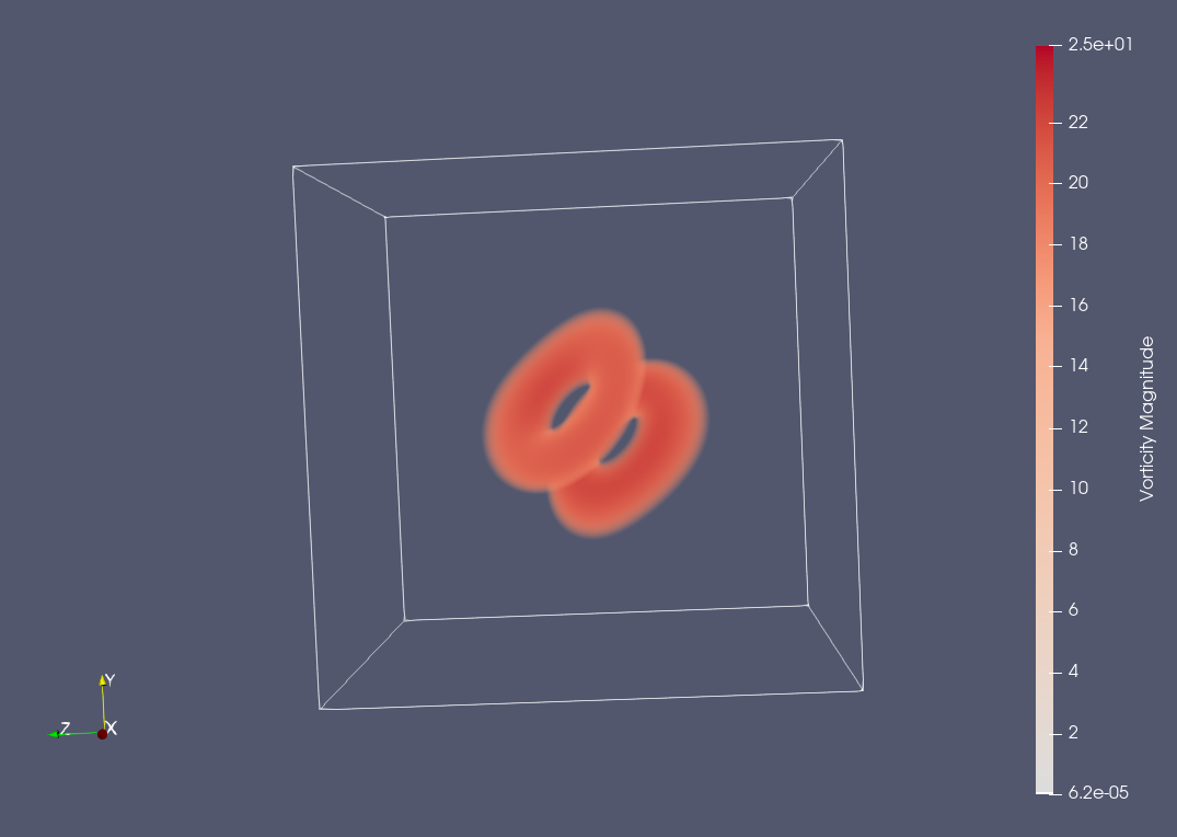
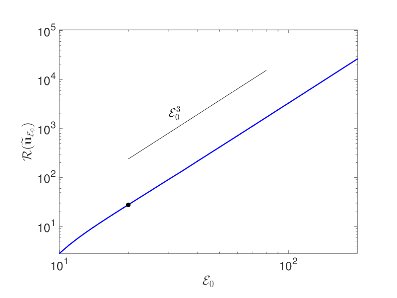
Figure 1: (a) Extreme vortex state $\widetilde{\mathbf{u}}_{{\mathcal{E}}_{0}}$ obtained by Ayala & Protas (2017), see also Lu & Doering (2008), as a solution of the instantaneous optimization Problem 2.1 for ${\mathcal{E}}_{0}=20$; shades of red correspond to the magnitude of the vorticity $|\left(\boldsymbol{\nabla}\times\widetilde{\mathbf{u}}_{{\mathcal{E}}_{0}}\right)({\mathbf{x}})|$ (see the color bar). (b) The maximum rate of growth of enstrophy ${\mathcal{R}}(\widetilde{\mathbf{u}}_{{\mathcal{E}}_{0}})$ as a function of the enstrophy ${\mathcal{E}}_{0}$ (the black solid symbol corresponds to the value of ${\mathcal{E}}_{0}$ characterizing the extreme vortex state shown in panel (a)).

In addition to sharpness under worst-case conditions, another question pertaining to inequality (10) is whether the upper bound on its RHS can also be realized under generic conditions in turbulent flows. This problem was studied by Schumacher et al. (2010) who demonstrated that in turbulent flows the rate of change of ensemble-averaged squared vorticity grows at most as $\frac{d}{dt}\langle\boldsymbol{\omega}^{2}\rangle\sim\langle\boldsymbol{\omega}^{2}\rangle^{3/2}$, where $\langle\cdot\rangle$ denotes ensemble averaging. This observation is consistent with the statistical theory of turbulence, more specifically, the Kármán-Howarth equation (Davidson, 2004).

The key conclusion from the results recalled above is that if a significant, let alone unbounded, growth of enstrophy is to be achieved in finite time, it must be associated with initial data ${\mathbf{u}}_{0}$ other than the extreme vortex states $\widetilde{\mathbf{u}}_{{\mathcal{E}}_{0}}$ saturating the upper bound in estimate (10) on the instantaneous rate of growth of enstrophy, cf. figure 1. More specifically, assuming the instantaneous rate of growth of enstrophy in the form $d{\mathcal{E}}/dt=C\,{\mathcal{E}}^{\alpha}$ for some prefactor $C>0$, any exponent $\alpha>2$ will lead to blow-up of ${\mathcal{E}}({\mathbf{u}}(t))$ at some finite time $t_{0}=t_{0}(\alpha)$ if this rate of growth is sustained over the interval $[0,t_{0})$. The fact that there is no blow-up when $1<\alpha\leq 2$ follows from the observation that one factor of ${\mathcal{E}}$ in (10) can be bounded in terms of the initial energy ${\mathcal{K}}_{0}:={\mathcal{K}}({\mathbf{u}}_{0})$ using (8a) as follows

$$\int_{0}^{t}{\mathcal{E}}({\mathbf{u}}(s))\,ds=\frac{1}{2\nu}\left[{\mathcal{K}}_{0}-{\mathcal{K}}({\mathbf{u}}(t))\right]\leq\frac{1}{2\nu}{\mathcal{K}}_{0},$$ (13)

which upon employing Grönwall’s lemma yields the bound

$$\max_{0\leq t\leq T}{\mathcal{E}}({\mathbf{u}}(t))\leq{\mathcal{E}}_{0}\,\exp\left[\int_{0}^{T}{\mathcal{E}}({\mathbf{u}}(s))\,ds\right]\leq{\mathcal{E}}_{0}\,\exp\left[\frac{1}{2\nu}{\mathcal{K}}_{0}\right]$$ (14)

valid for $0\leq\alpha\leq 2$. Evidently, as the rate of growth of enstrophy slows down and $\alpha\rightarrow 2^{+}$, for blow-up to occur a certain minimum growth rate must be sustained over windows of time with increasing length, i.e., $t_{0}\rightarrow\infty$. To assess the feasibility of such a scenario, in the next section we introduce an optimization approach which will allow us to systematically search for worst-case flow evolutions producing the maximum possible growth of enstrophy in finite time.

3 Maximization Problem

In order to probe the upper bound in estimate (11) for realizability, our objective in this section is to construct initial data $\widetilde{\mathbf{u}}_{0;{\mathcal{E}}_{0},T}$ for the Navier-Stokes system (2) with the prescribed enstrophy ${\mathcal{E}}_{0}>0$, such that at the given time $T>0$ the corresponding flow evolution will produce the maximum possible value of enstrophy ${\mathcal{E}}({\mathbf{u}}(T))$ under the assumption that the Navier-Stokes system admits smooth (classical) solutions on the time interval $(0,T]$. Defining the objective function ${\mathcal{E}}_{T}\;:\;H^{1}(\Omega)\rightarrow{\mathbb{R}}_{+}$, where

$${\mathcal{E}}_{T}({\mathbf{u}}_{0}):={\mathcal{E}}({\mathbf{u}}(T))=\frac{1}{2}\int_{\Omega}|\boldsymbol{\nabla}\times{\mathbf{u}}(T,{\mathbf{x}})|^{2}\,d{\mathbf{x}},$$ (15)

we thus arrive at the following

Problem 3.1

Given ${\mathcal{E}}_{0},T\in\mathbb{R}_{+}$ and the objective functional ${\mathcal{E}}_{T}({\mathbf{u}}_{0})$ from equation (15), find

$$\widetilde{\mathbf{u}}_{0;{\mathcal{E}}_{0},T} =\mathop{\arg\max}_{{\mathbf{u}}_{0}\in{\mathcal{Q}}_{{\mathcal{E}}_{0}}}\,{\mathcal{E}}_{T}({\mathbf{u}}_{0}),\quad\text{where}$$

$${\mathcal{Q}}_{{\mathcal{E}}_{0}} =\left\{{\mathbf{u}}\in H^{1}(\Omega)\,\colon\,\boldsymbol{\nabla}\cdot{\mathbf{u}}=0,\;{\mathcal{E}}({\mathbf{u}})={\mathcal{E}}_{0}\right\},$$

where $H^{1}(\Omega)$ denotes the Sobolev space of functions with square-integrable derivatives endowed with the inner product (Adams & Fournier, 2005)

$$\forall\,\mathbf{z}_{1},\mathbf{z}_{2}\in H^{1}(\Omega)\qquad\Big{\langle}\mathbf{z}_{1},\mathbf{z}_{2}\Big{\rangle}_{H^{1}(\Omega)}=\int_{\Omega}\mathbf{z}_{1}\cdot\mathbf{z}_{2}+\ell_{1}^{2}\,\boldsymbol{\nabla}\mathbf{z}_{1}\colon\boldsymbol{\nabla}\mathbf{z}_{2}\,d{\mathbf{x}},$$ (16)

where $\ell_{1}\in{\mathbb{R}}_{+}$ is a parameter with the meaning of a characteristic length scale (the reasons for introducing this parameter in the definition of the inner product will become clear below). The inner product in the space $L^{2}(\Omega)$ is obtained from (16) by setting $\ell_{1}=0$. The maximizers in Problem 3.1 are constrained to belong to the manifold ${\mathcal{Q}}_{{\mathcal{E}}_{0}}$ which represents the intersection of the subspace of divergence-free vector fields $(\boldsymbol{\nabla}\cdot{\mathbf{u}}=0)$ and a nonlinear manifold defined by the enstrophy constraint $({\mathcal{E}}({\mathbf{u}})={\mathcal{E}}_{0})$ in the Sobolev space $H^{1}(\Omega)$, where the smoothness requirement is necessary to ensure that the initial enstrophy ${\mathcal{E}}({\mathbf{u}}_{0})$ is well defined. Without loss of generality, we assume that $\int_{\Omega}{\mathbf{u}}_{0}\,d{\mathbf{x}}={\mathbf{0}}$, a property which is also invariant during the flow evolution. The fact that Problem 3.1 admits solutions is a consequence of the assumption that with the given parameters ${\mathcal{E}}_{0}$ and $T$ solutions of the Navier-Stokes system (2) are smooth on the time interval $[0,T]$.

The key insight we seek to deduce is how the maximum growth of enstrophy $\max_{T>0}\,{\mathcal{E}}_{T}(\widetilde{\mathbf{u}}_{0;{\mathcal{E}}_{0},T})$ obtained for time intervals $(0,T]$ with different lengths $0<T<\infty$ scales with the initial enstrophy ${\mathcal{E}}_{0}$. In order to evaluate this quantity for a given value of the initial enstrophy ${\mathcal{E}}_{0}$, we thus need to solve Problem 3.1 for different values of $T\in(0,T_{\text{max}}]$, where $T_{\text{max}}<\infty$ is the maximum considered length of the time interval, and with fixed ${\mathcal{E}}_{0}$, so that the maximum with respect to $T$ can be evaluated. We note that this approach is justified by the existence of bounds (expressed in terms of norms of the initial data ${\mathbf{u}}_{0}$ and viscosity $\nu$) on the largest time $T_{\text{max}}$ when a singularity might occur (Ohkitani, 2016). Assuming that the optimal initial data $\widetilde{\mathbf{u}}_{0;{\mathcal{E}}_{0},T}$ obtained as solution of Problem 3.1 has (at least piecewise) continuous dependence on the parameter $T$, we will refer to the mapping $T\longmapsto\widetilde{\mathbf{u}}_{0;{\mathcal{E}}_{0},T}$ with ${\mathcal{E}}_{0}$ fixed as a “maximizing branch”.

In order to solve Problem 3.1 for given values of ${\mathcal{E}}_{0}$ and $T$ we adopt an “optimize-then-discretize” approach (Gunzburger, 2003) in which a gradient method is first formulated in the infinite-dimensional (continuous) setting and only then the resulting equations and expressions are discretized for the purpose of numerical solution. An essentially identical approach was used by Ayala & Protas (2011) to solve an optimization problem analogous to Problem 3.1, but formulated for the 1D Burgers equation. The maximizer $\widetilde{\mathbf{u}}_{0;{\mathcal{E}}_{0},T}$ can be found as $\widetilde{\mathbf{u}}_{0;{\mathcal{E}}_{0},T}=\lim_{n\rightarrow\infty}\mathbf{u}_{0;{\mathcal{E}}_{0},T}^{(n)}$ using the following iterative procedure representing a discretization of a gradient flow projected on $\mathcal{Q}_{{\mathcal{E}}_{0}}$

$$\mathbf{u}_{0;{\mathcal{E}}_{0},T}^{(n+1)} =\mathbb{P}_{\mathcal{Q}_{{\mathcal{E}}_{0}}}\left(\;\mathbf{u}_{0;{\mathcal{E}}_{0},T}^{(n)}+\tau_{n}\nabla{\mathcal{E}}_{T}\left(\mathbf{u}_{0;{\mathcal{E}}_{0},T}^{(n)}\right)\;\right),$$ (17)

$$\mathbf{u}_{0;{\mathcal{E}}_{0},T}^{(1)} ={\mathbf{u}}^{0},$$

where $\mathbf{u}_{0;{\mathcal{E}}_{0},T}^{(n)}$ is an approximation of the maximizer obtained at the $n$-th iteration, $\mathbb{P}_{\mathcal{Q}_{{\mathcal{E}}_{0}}}\;:\;H^{1}(\Omega)\rightarrow{\mathcal{Q}}_{{\mathcal{E}}_{0}}$ is the projection operator, ${\mathbf{u}}^{0}$ is the initial guess and $\tau_{n}$ is the length of the step. A key element of the iterative procedure (17) is the evaluation of the gradient $\nabla{\mathcal{E}}_{T}({\mathbf{u}}_{0})$ of the objective functional ${\mathcal{E}}_{T}({\mathbf{u}}_{0})$, cf. (15), representing its (infinite-dimensional) sensitivity to perturbations of the initial data ${\mathbf{u}}_{0}$ in the governing system (2). We emphasize that it is essential for the gradient to possess the required regularity, namely, $\nabla{\mathcal{E}}_{T}({\mathbf{u}}_{0})\in H^{1}(\Omega)$.

The first step to determine the gradient $\nabla{\mathcal{E}}_{T}({\mathbf{u}}_{0})$ is to consider the Gâteaux (directional) differential ${\mathcal{E}}^{\prime}_{T}({\mathbf{u}}_{0};\cdot)\;:\;H^{1}(\Omega)\rightarrow{\mathbb{R}}$ of the objective functional ${\mathcal{E}}_{T}({\mathbf{u}}_{0})$ defined as ${\mathcal{E}}^{\prime}_{T}({\mathbf{u}}_{0};{\mathbf{u}}_{0}^{\prime})=\lim_{\epsilon\rightarrow 0}\epsilon^{-1}\left[{\mathcal{E}}_{T}({\mathbf{u}}_{0}+\epsilon{\mathbf{u}}_{0}^{\prime})-{\mathcal{E}}_{T}({\mathbf{u}}_{0})\right]$ for some arbitrary perturbation ${\mathbf{u}}_{0}^{\prime}\in H^{1}(\Omega)$. The gradient $\nabla{\mathcal{E}}_{T}({\mathbf{u}}_{0})$ can then be extracted from the Gâteaux differential ${\mathcal{E}}^{\prime}_{T}({\mathbf{u}}_{0};{\mathbf{u}}_{0}^{\prime})$ recognizing that, when viewed as a function of its second argument, this differential is a bounded linear functional on the space $H^{1}(\Omega)$ and we can therefore invoke the Riesz representation theorem (Luenberger, 1969)

$${\mathcal{E}}^{\prime}_{T}({\mathbf{u}}_{0};{\mathbf{u}}_{0}^{\prime})=\Big{\langle}\nabla^{L_{2}}{\mathcal{E}}_{T}({\mathbf{u}}_{0}),{\mathbf{u}}_{0}^{\prime}\Big{\rangle}_{L^{2}(\Omega)}=\Big{\langle}\nabla{\mathcal{E}}_{T}({\mathbf{u}}_{0}),{\mathbf{u}}_{0}^{\prime}\Big{\rangle}_{H^{1}(\Omega)},$$ (18)

where the gradient $\nabla{\mathcal{E}}_{T}({\mathbf{u}}_{0})$ is the Riesz representer in the function space $H^{1}(\Omega)$. In (18) we also formally defined the gradient $\nabla^{L_{2}}{\mathcal{E}}_{T}({\mathbf{u}}_{0})$ computed with respect to the $L^{2}$ topology as it will be useful in subsequent computations. Given the definition of the objective functional in (15), its Gâteaux differential can be expressed as

$${\mathcal{E}}^{\prime}_{T}({\mathbf{u}}_{0};{\mathbf{u}}_{0}^{\prime})=\int_{\Omega}(\boldsymbol{\nabla}\times{\mathbf{u}}(T,{\mathbf{x}}))\cdot(\boldsymbol{\nabla}\times{\mathbf{u}}^{\prime}(T,{\mathbf{x}}))\,d{\mathbf{x}}=\int_{\Omega}\boldsymbol{\Delta}{\mathbf{u}}(T,{\mathbf{x}}))\cdot{\mathbf{u}}^{\prime}(T,{\mathbf{x}})\,d{\mathbf{x}},$$ (19)

where the last equality follows from integration by parts and the vector identity $\boldsymbol{\nabla}\times(\boldsymbol{\nabla}\times{\mathbf{z}})=\boldsymbol{\nabla}(\boldsymbol{\nabla}\cdot{\mathbf{z}})-\boldsymbol{\Delta}{\mathbf{z}}$, whereas the perturbation field ${\mathbf{u}}^{\prime}={\mathbf{u}}^{\prime}(t,{\mathbf{x}})$ is a solution of the Navier-Stokes system linearized around the trajectory corresponding to the initial data ${\mathbf{u}}_{0}$ (Gunzburger, 2003), i.e.,

$${\mathcal{L}}\begin{bmatrix}{\mathbf{u}}^{\prime}\\ p^{\prime}\end{bmatrix}:= \begin{bmatrix}\partial_{t}{\mathbf{u}}^{\prime}+{\mathbf{u}}^{\prime}\cdot\boldsymbol{\nabla}{\mathbf{u}}+{\mathbf{u}}\cdot\boldsymbol{\nabla}{\mathbf{u}}^{\prime}+\boldsymbol{\nabla}p^{\prime}-\nu\boldsymbol{\Delta}{\mathbf{u}}^{\prime}\\ \boldsymbol{\nabla}\cdot{\mathbf{u}}^{\prime}\end{bmatrix}=\begin{bmatrix}\mathbf{0}\\ 0\end{bmatrix},$$ (20a)

$${\mathbf{u}}^{\prime}(0)= {\mathbf{u}}_{0}^{\prime}$$ (20b)

which is subject to the periodic boundary conditions and where $p^{\prime}$ is the perturbation pressure.

We note that expression (19) for the Gâteaux differential is not consistent with the Riesz form (18), because the perturbation ${\mathbf{u}}_{0}^{\prime}$ of the initial data does not appear in it explicitly as a factor, but is instead hidden as the initial condition in the linearized problem, cf. (20b). In order to transform (19) to the Riesz form, we introduce the adjoint states ${\mathbf{u}}^{*}\;:\;[0,T]\times\Omega\rightarrow{\mathbb{R}}^{3}$ and $p^{*}\;:\;[0,T]\times\Omega\rightarrow{\mathbb{R}}$, and the following duality-pairing relation

$$\left({\mathcal{L}}\begin{bmatrix}{\mathbf{u}}^{\prime}\\ p^{\prime}\end{bmatrix},\begin{bmatrix}{\mathbf{u}}^{*}\\ p^{*}\end{bmatrix}\right):= \int_{0}^{T}\int_{\Omega}{\mathcal{L}}\begin{bmatrix}{\mathbf{u}}^{\prime}\\ p^{\prime}\end{bmatrix}\cdot\begin{bmatrix}{\mathbf{u}}^{*}\\ p^{*}\end{bmatrix}\,d{\mathbf{x}}\,dt=\left(\begin{bmatrix}{\mathbf{u}}^{\prime}\\ p^{\prime}\end{bmatrix},{\mathcal{L}}^{*}\begin{bmatrix}{\mathbf{u}}^{*}\\ p^{*}\end{bmatrix}\right)+$$ (21)

$${\underbrace{\int_{\Omega}{\mathbf{u}}^{\prime}(T,{\mathbf{x}})\cdot{\mathbf{u}}^{*}(T,{\mathbf{x}})\,d{\mathbf{x}}}_{{\mathcal{E}}^{\prime}_{T}({\mathbf{u}}_{0};{\mathbf{u}}_{0}^{\prime})}}-\int_{\Omega}{\mathbf{u}}^{\prime}(0,{\mathbf{x}})\cdot{\mathbf{u}}^{*}(0,{\mathbf{x}})\,d{\mathbf{x}}=0,$$

where “$\cdot$” in the first integrand expression denotes the Euclidean dot product evaluated at $(t,{\mathbf{x}})$. Performing integration by parts with respect to both space and time then allows us to define the adjoint system as

$${\mathcal{L}}^{*}\begin{bmatrix}{\mathbf{u}}^{*}\\ p^{*}\end{bmatrix}:= \begin{bmatrix}-\partial_{t}{\mathbf{u}}^{*}-\left[\boldsymbol{\nabla}{\mathbf{u}}^{*}+\left(\boldsymbol{\nabla}{\mathbf{u}}^{*}\right)^{T}\right]{\mathbf{u}}-\boldsymbol{\nabla}p^{*}-\nu\boldsymbol{\Delta}{\mathbf{u}}^{*}\\ -\boldsymbol{\nabla}\cdot{\mathbf{u}}^{*}\end{bmatrix}=\begin{bmatrix}{\mathbf{0}}\\ 0\end{bmatrix},$$ (22a)

$${\mathbf{u}}^{*}(T)= {\boldsymbol{\Delta}{\mathbf{u}}}$$ (22b)

which is also subject to the periodic boundary conditions. We note that in identity (21) all boundary terms resulting from integration by parts with respect to the space variables vanish due to the periodic boundary conditions. The term $\int_{\Omega}{\mathbf{u}}^{\prime}(T,{\mathbf{x}})\cdot{\mathbf{u}}^{*}(T,{\mathbf{x}})\,d{\mathbf{x}}$ resulting from integration by parts with respect to time is equal to the Gâteaux differential (19) due to the judicious choice of the terminal condition (22b), such that identity (21) implies

$${\mathcal{E}}^{\prime}_{T}({\mathbf{u}}_{0};{\mathbf{u}}_{0}^{\prime})=\int_{\Omega}{\mathbf{u}}^{\prime}_{0}({\mathbf{x}})\cdot{\mathbf{u}}^{*}(0,{\mathbf{x}})\,d{\mathbf{x}}.$$ (23)

Applying the first equality in Riesz relations (18) to (23) we obtain the $L^{2}$ gradient as

$$\nabla^{L^{2}}{\mathcal{E}}_{T}({\mathbf{u}}_{0})={\mathbf{u}}^{*}(0).$$ (24)

In order to obtain the required Sobolev $H^{1}$ gradient $\nabla{\mathcal{E}}_{T}({\mathbf{u}}_{0})$, we identify the Gâteaux differential in (23) with the $H^{1}$ inner product, cf. (16). Then, recognizing that the perturbations ${\mathbf{u}}_{0}^{\prime}$ are arbitrary, we obtain the following elliptic boundary-value problem (Protas et al., 2004)

$$\left[\operatorname{Id}\,-\,\ell_{1}^{2}\,\boldsymbol{\Delta}\right]\nabla{\mathcal{E}}_{T}({\mathbf{u}}_{0})=\nabla^{L_{2}}{\mathcal{E}}_{T}({\mathbf{u}}_{0})\qquad\text{in}\ \Omega$$ (25)

subject to the periodic boundary conditions, which must be solved to determine $\nabla{\mathcal{E}}_{T}({\mathbf{u}}_{0})$. The gradient fields $\nabla^{L_{2}}{\mathcal{E}}_{T}({\mathbf{u}}_{0})$ and $\nabla{\mathcal{E}}_{T}({\mathbf{u}}_{0})$ can be interpreted as infinite-dimensional sensitivities of the objective functional ${\mathcal{E}}_{T}({\mathbf{u}}_{0})$, cf. (15), with respect to perturbations of the initial data ${\mathbf{u}}_{0}$. While these two gradients may point towards the same local maximizer, they represent distinct “directions”, since they are defined with respect to different norms ($L^{2}$ vs. $H^{1}$). As shown by Protas et al. (2004), extraction of gradients in spaces of smoother functions such as $H^{1}(\Omega)$ can be interpreted as low-pass filtering of the $L^{2}$ gradients with the parameter $\ell_{1}$ acting as the cut-off length-scale. Although Sobolev gradients obtained with different $0<\ell_{1}<\infty$ are equivalent, in the precise sense of norm equivalence (Berger, 1977), the value of $\ell_{1}$ tends to have a significant effect on the rate of convergence of gradient iterations (17) (Protas et al., 2004) and the choice of its numerical value will be discussed in §4. We emphasize that, while the $H^{1}$ gradient is used exclusively in the actual computations, cf. (17), the $L^{2}$ gradient is computed first merely as an intermediate step.

Evaluation of the $L^{2}$ gradient at a given iteration via (24) requires solution of the Navier-Stokes system (2) followed by solution of the adjoint system (22). We note that this system is a linear problem with coefficients and the terminal condition determined by the solution of the Navier-Stokes system obtained earlier during the iteration. The adjoint system (22) is a terminal value problem, implying that it must be integrated backwards in time from $t=T$ to $t=0$ (since the term with the time derivative has a negative sign, this problem is well posed). Once the $L^{2}$ gradient is determined using (24), the corresponding Sobolev $H^{1}$ gradient can be obtained by solving problem (25). We add that the thus computed gradient satisfies the divergence-free condition by construction, i.e., $\boldsymbol{\nabla}\cdot(\nabla{\mathcal{E}}_{T}({\mathbf{u}}_{0}))=0$.

As regards the fixed-enstrophy constraint ${\mathcal{E}}({\mathbf{u}}_{0})={\mathcal{E}}_{0}$, this property is enforced in iterations (17) using the projection operator $\mathbb{P}_{\mathcal{Q}_{{\mathcal{E}}_{0}}}$ defined as the normalization

$$\mathbb{P}_{{\mathcal{Q}}_{{\mathcal{E}}_{0}}}({\mathbf{u}}_{0}):=\sqrt{\frac{{\mathcal{E}}_{0}}{{\mathcal{E}}({\mathbf{u}}_{0})}}\,{\mathbf{u}}_{0}$$ (26)

which clearly preserves the divergence-free property of the argument.

The step size $\tau_{n}$ in algorithm (17) is computed as

$$\tau_{n}=\mathop{\operatorname{argmax}}_{\tau>0}\left\{{\mathcal{E}}_{T}\left[\mathbb{P}_{{\mathcal{Q}}_{{\mathcal{E}}_{0}}}\left(\;\mathbf{u}_{0;{\mathcal{E}}_{0},T}^{(n)}+\tau\,\nabla{\mathcal{E}}_{T}(\mathbf{u}_{0;{\mathcal{E}}_{0},T}^{(n)})\;\right)\right]\right\}$$ (27)

which is done using a suitable derivative-free line-search approach, such as a variant of Brent’s algorithm (Nocedal & Wright, 1999; Press et al., 1986). Equation (27) can be interpreted as a modification of the standard line-search problem where optimization is performed following an arc (a geodesic in the limit of infinitesimal step sizes) lying on the constraint manifold $\mathcal{S}_{{\mathcal{E}}_{0}}$, rather than along a straight line. This approach was already successfully employed to solve similar problems in Ayala & Protas (2011, 2014a, 2017).

Maximizing branches are computed using a continuation approach by fixing one parameter, e.g., ${\mathcal{E}}_{0}$, and then solving Problem 3.1 with procedure (17) repeatedly for increasing values of $T$. In this process the maximizer $\widetilde{\mathbf{u}}_{0;{\mathcal{E}}_{0},T}$ obtained for some ${\mathcal{E}}_{0}$ and $T$ is employed as the initial guess ${\mathbf{u}}^{0}$ in (17) to compute the maximizer $\widetilde{{\mathbf{u}}}_{0;{\mathcal{E}}_{0},T+\Delta T}$ on a larger time interval $[0,T+\Delta T]$, or $\widetilde{{\mathbf{u}}}_{0;{\mathcal{E}}_{0}+\Delta{\mathcal{E}}_{0},T}$ for a larger initial enstrophy ${\mathcal{E}}_{0}+\Delta{\mathcal{E}}_{0}$, for some sufficiently small $\Delta T$ or $\Delta{\mathcal{E}}_{0}$. Since in the limit $T\rightarrow 0$ solutions of the finite-time optimization Problem 3.1 coincide with the solutions of the instantaneous optimization Problem 2.1, for small initial enstrophy values ${\mathcal{E}}_{0}$ the instantaneous maximizers $\widetilde{\mathbf{u}}_{{\mathcal{E}}_{0}}$, cf. figure 1, are used as “seeds” to initiate the computation of the maximizing branch for the given value of ${\mathcal{E}}_{0}$, i.e., as the initial guess for $\widetilde{{\mathbf{u}}}_{0;{\mathcal{E}}_{0},\Delta T}$. The procedure outlined above is summarized as Algorithm 1. For larger initial enstrophy values it is also convenient to perform continuation with respect to ${\mathcal{E}}_{0}$ with $T$ fixed and in such case an essentially the same procedure applies, except that the order of the two outermost “repeat” loops in Algorithm 1 is reversed. While there exist alternatives to the continuation approach, provided $\Delta{\mathcal{E}}_{0}$ and $\Delta T$ are sufficiently small, this technique in fact results in the fastest convergence of iterations (17) and also ensures that computed optimal initial data lie on a maximizing branch.

  

  set ${\mathcal{E}}_{0}=0$, $T=0$

  repeat

     {———————— loop over increasing enstrophy values ${\mathcal{E}}_{0}$ ————————}

     ${\mathcal{E}}_{0}={\mathcal{E}}_{0}+\Delta{\mathcal{E}}$

     compute $\widetilde{\mathbf{u}}_{{\mathcal{E}}_{0}}$ by solving Problem 2.1, as described in Ayala & Protas (2017)

     $\mathbf{u}_{0;{\mathcal{E}}_{0},T}^{(0)}=\widetilde{\mathbf{u}}_{{\mathcal{E}}_{0}}$

     repeat

        {———————— loop over expanding time intervals $T$ ————————–}

        $T=T+\Delta T$

        $n=0$

        compute $e_{0}={\mathcal{E}}_{T}\left(\mathbf{u}_{0;{\mathcal{E}}_{0},T}^{(0)}\right)$

        repeat

           {————————— optimization iterations (17) ——————————–}

           solve the Navier-Stokes system with initial condition $\mathbf{u}_{0;{\mathcal{E}}_{0},T}^{(n)}$, see equation (2)

           solve the adjoint system to obtain ${\mathbf{u}}^{*}$ and $p^{*}$, see equation (22)

           compute the $L^{2}$ gradient $\nabla^{L_{2}}{\mathcal{E}}_{T}\left(\mathbf{u}_{0;{\mathcal{E}}_{0},T}^{(n)}\right)$, see equation (24)

           compute the Sobolev gradient $\nabla{\mathcal{E}}_{T}\left(\mathbf{u}_{0;{\mathcal{E}}_{0},T}^{(n)}\right)$, see equation (25)

           compute the optimal step size $\tau_{n}$, see equation (27)

           set $\mathbf{u}_{0;{\mathcal{E}}_{0},T}^{(n+1)}=\mathbb{P}_{{\mathcal{Q}}_{{\mathcal{E}}_{0}}}\left(\;\mathbf{u}_{0;{\mathcal{E}}_{0},T}^{(n)}+\tau_{n}\nabla{\mathcal{E}}_{T}\left(\mathbf{u}_{0;{\mathcal{E}}_{0},T}^{(n)}\right)\;\right)$, see equations (26)

           set $e_{1}={\mathcal{E}}_{T}\left(\mathbf{u}_{0;{\mathcal{E}}_{0},T}^{(n+1)}\right)$

           compute relative_change $=(e_{1}-e_{0})/e_{0}$

           set $e_{0}=e_{1}$

           set $n=n+1$

        until   relative_change $<$ $\epsilon$

        $\widetilde{\mathbf{u}}_{0;{\mathcal{E}}_{0},T}=\mathbf{u}_{0;{\mathcal{E}}_{0},T}^{(n+1)}$

        $\mathbf{u}_{0;{\mathcal{E}}_{0},T}^{(0)}=\widetilde{\mathbf{u}}_{0;{\mathcal{E}}_{0},T}$

     until  $T>T_{\text{max}}$

  until  ${\mathcal{E}}_{0}>{\mathcal{E}}_{\text{max}}$

Algorithm 1 Computation of maximizing branches parameterized by $T$ for different ${\mathcal{E}}_{0}$ using continuation approach.
Input:
   ${\mathcal{E}}_{\text{max}}$ — maximum enstrophy
   $T_{\text{max}}$ — maximum time interval
   $\Delta{\mathcal{E}}$ — (adjustable) increment of enstrophy
   $\Delta T$ — (adjustable) increment of the length of the time interval
   $\epsilon$ — tolerance in the solution of optimization problem 3.1 via iterations (17)
   $\ell_{1}$ — adjustable length scale defining inner product (16), see also (25)
Output:
   branches of optimal initial data $\widetilde{\mathbf{u}}_{0;{\mathcal{E}}_{0},T}$,  $0\leq{\mathcal{E}}_{0}\leq{\mathcal{E}}_{\text{max}}$, $0\leq T\leq T_{\text{max}}$,

Finally, we remark that the “optimize-then-discretize” approach adopted here has the key advantage that in such a continuous formulation the expressions representing the sensitivity of the objective functional ${\mathcal{E}}_{T}({\mathbf{u}}_{0})$, i.e., the gradients $\nabla^{L_{2}}{\mathcal{E}}_{T}({\mathbf{u}}_{0})$ and $\nabla{\mathcal{E}}_{T}({\mathbf{u}}_{0})$, are independent of the specific discretization approach chosen to evaluate them. This should be contrasted with the discrete (“discretize-then-optimize”) formulation, where a change of the discretization method would require rederivation of the gradient expressions. In addition, the continuous formulation allows us to strictly enforce the regularity of maximizers required in Problem 3.1. Last, but not least, the continuous formulation is also arguably better adapted to study problems motivated by questions in mathematical analysis such as the problems considered here. Our strategy for the numerical implementation of the different elements of Algorithm 1 is presented in the next section.

4 Numerical Approach

In this section we briefly describe the key elements of the numerical approach used to implement Algorithm 1 and also comment on the validation strategies we employed. Evaluation of the objective functional (15) requires solution of the Navier-Stokes system (2) on the time interval $[0,T]$ with the given initial data ${\mathbf{u}}_{0}$. This system is solved numerically with an approach combining a pseudo-spectral approximation of spatial derivatives with a fourth-order semi-implicit Runge-Kutta method (Bewley, 2009) used to discretize the problem in time. In the evaluation of the nonlinear term dealiasing is performed using the Gaussian filtering approach proposed by Hou & Li (2007). Massively parallel implementation based on MPI and using the fftw routines (Frigo & Johnson, 2003) to perform Fourier transforms allowed us to employ resolutions varying from $128^{3}$ to $512^{3}$ in the low-enstrophy and high-enstrophy cases, respectively. Solution of optimization problem 3.1 for a large initial enstrophy ${\mathcal{E}}_{0}\lessapprox 1000$ and an intermediate length $T$ of the time interval typically required a computational time of ${\mathcal{O}}(10^{2})$ hours on ${\mathcal{O}}(10^{2})$ CPU cores. A number of different diagnostics were checked to ensure that all flow solutions discussed in §5 are well resolved. We refer the reader to the dissertation by Ayala (2014) for additional details and a validation of this approach.

In addition to the Navier-Stokes system (2), evaluation of the $L^{2}$ gradient (24) also requires solution of the adjoint system (22). This problem is solved using essentially the same numerical approach as used to solve the Navier-Stokes system (2). The velocity field ${\mathbf{u}}={\mathbf{u}}(t,{\mathbf{x}})$ needed to evaluate the coefficients and the terminal condition in the adjoint system is saved at discrete time levels during solution of the Navier-Stokes system (since the considered time intervals $[0,T]$ are not very long, data for entire flow evolutions could be stored with our available temporary storage resources). The accuracy of the evaluation of the gradient $\nabla^{L^{2}}{\mathcal{E}}_{T}({\mathbf{u}}_{0})$ determined as described in §3 is verified by examining the quantity $\kappa(\epsilon):=\epsilon^{-1}\left[{\mathcal{E}}_{T}({\mathbf{u}}_{0}+\epsilon{\mathbf{u}}_{0}^{\prime})-{\mathcal{E}}_{T}({\mathbf{u}}_{0})\right]/\langle\nabla^{L_{2}}{\mathcal{E}}_{T}({\mathbf{u}}_{0}),{\mathbf{u}}_{0}^{\prime}\rangle_{L^{2}(\Omega)}$ which represents the ratio of a forward finite-difference approximation of the Gâteaux differential ${\mathcal{E}}^{\prime}_{T}({\mathbf{u}}_{0};{\mathbf{u}}_{0}^{\prime})$ and its expression given in terms of the Riesz formula (18) with the gradient given in (24). The evaluation of gradients is validated when $\kappa(\epsilon)\approx 1$ for intermediate values of $\epsilon$ and different choices of ${\mathbf{u}}_{0}$ and ${\mathbf{u}}_{0}^{\prime}$. For such intermediate values of $\epsilon$ we observe that, as expected, $|\kappa(\epsilon)-1|$ is reduced as the numerical discretization parameters are refined (when $\epsilon\rightarrow 0$, $|\kappa(\epsilon)|$ becomes unbounded as a result of round-off errors due to subtractive cancellation, whereas when $\epsilon$ is large $\kappa(\epsilon)$ deviates from unity because of truncation errors in the finite-difference approximation of the Gâteaux differential, both of which are well-known effects (Ayala, 2014)).

As regards the computation of the Sobolev $H^{1}$ gradients, cf. (25), the parameter $\ell_{1}$ is adjusted during the optimization iterations and is chosen so that $\ell_{1}\in[\ell_{\min},\ell_{\max}]$, where $\ell_{\min}$ is the length scale associated with the spatial resolution $N=128,256,512$ used for computations and $\ell_{\max}$ is the characteristic length scale of the domain $\Omega$, that is, $\ell_{\min}\sim{\mathcal{O}}(1/N)$ and $\ell_{\max}\sim{\mathcal{O}}(1)$. We remark that, given the equivalence of the Sobolev inner products (16) corresponding to different values of $\ell_{1}$ (as long as $\ell_{1}\neq 0$), these choices do not affect the maximizers found, but only how rapidly they are approached by iterations (17). The computational results presented in the next section have been thoroughly validated to ensure they are converged with respect to refinement of the different numerical parameters discussed above.

5 Computational Results

In this section we proceed to present our computational results obtained by solving the finite-time optimization problem 3.1 for a broad range of initial enstrophies ${\mathcal{E}}_{0}$ and lengths $T$ of the time interval. The ultimate goal is to understand what is the largest growth of enstrophy possible under the 3D Navier-Stokes dynamics, in particular, whether this growth could saturate estimate (11) and become unbounded in finite time, then how this maximum growth depends on the initial enstrophy ${\mathcal{E}}_{0}$ and, finally, what is the flow mechanism realizing this extreme behavior. To address these questions we compute branches of maximizing solutions corresponding to different fixed values of the initial enstrophy ${\mathcal{E}}_{0}$ and increasing lengths $T$ of the time window. For smaller values of ${\mathcal{E}}_{0}$ this can be done using Algorithm 1 in which solutions of the instantaneous maximization problem 2.1 are used to initialize the computation of the maximizing branches for short optimization times $T$. Since for large initial enstrophy values (${\mathcal{E}}_{0}>100$), the instantaneous problem 2.1 is harder to solve because of increased resolution requirements (more on this below), in such cases it is more convenient to initiate computation of the new branches corresponding to increased values of ${\mathcal{E}}_{0}$ by performing continuation with respect to ${\mathcal{E}}_{0}$ for some intermediate values of $T$. Only then we can again perform continuation with respect to $T$ at a new fixed value of ${\mathcal{E}}_{0}$.

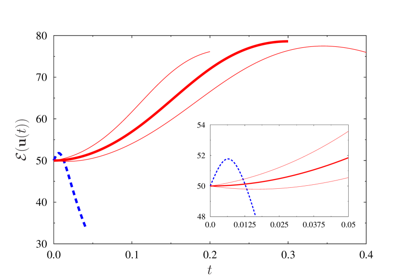
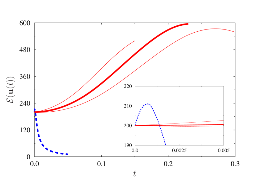
(a) ${\mathcal{E}}_{0}=50$, $T=0.2,0.3,0.4$ (b) ${\mathcal{E}}_{0}=200$, $T=0.15,0.23,0.3$

Figure 2: Enstrophy ${\mathcal{E}}({\mathbf{u}}(t))$ as a function of time $t$ obtained from the solution of the Navier-Stokes system (2) with the initial condition ${\mathbf{u}}_{0}$ given by (blue dashed line) the maximizer $\widetilde{\mathbf{u}}_{{\mathcal{E}}_{0}}$ of the instantaneous optimization problem 2.1 and (red solid lines) the maximizers $\widetilde{\mathbf{u}}_{0;{\mathcal{E}}_{0},T}$ of the finite-time optimization problem 3.1 for the indicated values of ${\mathcal{E}}_{0}$ and $T$ (the curves corresponding to the optimal lengths of the time window, $\widetilde{T}_{{\mathcal{E}}_{0}}=0.3$ for ${\mathcal{E}}_{0}=50$ and $\widetilde{T}_{{\mathcal{E}}_{0}}=0.23$ for ${\mathcal{E}}_{0}=200$, are marked with thick lines whereas the insets represent magnifications of the initial stages of evolution).

A typical time evolution of enstrophy ${\mathcal{E}}({\mathbf{u}}(t))$ is presented in figure 2 where we show the results produced by solving the Navier-Stokes system (2) with the initial data $\widetilde{\mathbf{u}}_{{\mathcal{E}}_{0}}$ and $\widetilde{\mathbf{u}}_{0;{\mathcal{E}}_{0},T}$ obtained as the solutions of the instantaneous and finite-time optimization problems 2.1 and 3.1 for ${\mathcal{E}}_{0}=50$ and ${\mathcal{E}}_{0}=200$, and different $T$. We note that when the instantaneously optimal initial data $\widetilde{\mathbf{u}}_{{\mathcal{E}}_{0}}$ is used, then the enstrophy grows very rapidly for short times which is followed by an immediate depletion of its growth, as already analyzed by Ayala & Protas (2017). On the other hand, when the optimal initial data $\widetilde{\mathbf{u}}_{0;{\mathcal{E}}_{0},T}$ obtained as solution of the finite-time optimization problem 3.1 with “long” time windows $T$ is used, then the enstrophy grows very slowly at first (or even decreases when $T$ is sufficiently large), but eventually a much larger growth is achieved at the end of the time window, i.e., at $t=T$. As is also evident from figure 2, when $T$ is sufficiently large, the enstrophy achieves a well-defined maximum as a function of time and there exists a value of $T$ for which the maximum enstrophy is achieved precisely at the end of the optimization window, i.e., for $t=T$. Clearly, this value, which we shall denote $\widetilde{T}_{{\mathcal{E}}_{0}}:=\mathop{\arg\max}_{T>0}{\mathcal{E}}_{T}(\widetilde{\mathbf{u}}_{0;{\mathcal{E}}_{0},T})$, defines the optimal length of the optimization interval in Problem 3.1 for which the largest maximum enstrophy is achieved for a given ${\mathcal{E}}_{0}$. Then, ${\mathcal{E}}_{T}(\widetilde{\mathbf{u}}_{0;{\mathcal{E}}_{0},\widetilde{T}_{{\mathcal{E}}_{0}}})=\max_{T>0}{\mathcal{E}}_{T}(\widetilde{\mathbf{u}}_{0;{\mathcal{E}}_{0},T})$ is the largest enstrophy achievable using an initial condition with enstrophy ${\mathcal{E}}_{0}$. Approximating the optimal length of the time interval $\widetilde{T}_{{\mathcal{E}}_{0}}$ for a given value of the initial enstrophy ${\mathcal{E}}_{0}$ requires solution of the finite-time optimization problem 3.1 for several different values of $T$.

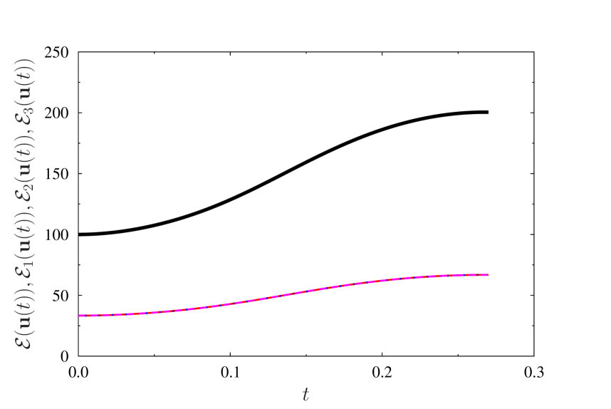
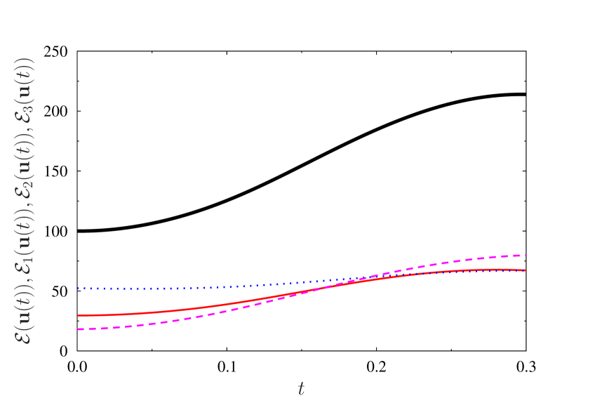
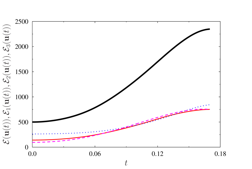
(a) ${\mathcal{E}}_{0}=100$, $\widetilde{T}_{{\mathcal{E}}_{0}}=0.27$ (symmetric) (b) ${\mathcal{E}}_{0}=100$, $\widetilde{T}_{{\mathcal{E}}_{0}}=0.27$ (asymmetric) (c) ${\mathcal{E}}_{0}=500$, $\widetilde{T}_{{\mathcal{E}}_{0}}=0.17$ (asymmetric) (d) ${\mathcal{E}}_{0}=1000$, $\widetilde{T}_{{\mathcal{E}}_{0}}=0.12$ (asymmetric)

Figure 3: Evolution of (black thick solid lines) the total enstrophy ${\mathcal{E}}({\mathbf{u}}(t))$ and its components (red thin solid lines) ${\mathcal{E}}_{1}({\mathbf{u}}(t))$, (blue dotted lines) ${\mathcal{E}}_{2}({\mathbf{u}}(t))$ and (pink dashed lines) ${\mathcal{E}}_{3}({\mathbf{u}}(t))$ in the solution of the Navier-Stokes system (2) with the optimal initial conditions $\widetilde{\mathbf{u}}_{0;{\mathcal{E}}_{0},T}$ obtained by solving the finite-time optimization problem 3.1 for the indicated values of ${\mathcal{E}}_{0}$ and $T$. Panels (a) and (b–d) correspond to the optimal initial conditions $\widetilde{\mathbf{u}}_{0;{\mathcal{E}}_{0},T}$ from the symmetric and asymmetric branch, respectively.

Closer inspection of the solutions to the Navier-Stokes system (2) corresponding to optimal initial condition $\widetilde{\mathbf{u}}_{0;{\mathcal{E}}_{0},T}$ obtained by solving problem 3.1 for ${\mathcal{E}}_{0}\lessapprox 100$ and ${\mathcal{E}}_{0}\gtrapprox 100$ indicates that these solutions have in fact distinct properties in terms of symmetry. To analyze this issue, in figure 3 we show the time histories of the enstrophy components ${\mathcal{E}}_{i}({\mathbf{u}}(t))$, $i=1,2,3$, associated with the three coordinate directions defined as

$${\mathcal{E}}_{i}({\mathbf{u}}(t)):=\int_{\Omega}\left|\left(\boldsymbol{\nabla}\times{\mathbf{u}}(t)\right)\cdot{\mathbf{e}}_{i}\right|^{2}\,d{\mathbf{x}},\quad i=1,2,3,$$ (28)

where ${\mathbf{e}}_{1}$, ${\mathbf{e}}_{2}$, ${\mathbf{e}}_{3}$ are the unit vectors of the Cartesian coordinate system and we have the obvious identity $\forall t\ \ {\mathcal{E}}({\mathbf{u}}(t))=\sum_{i=1}^{3}{\mathcal{E}}_{i}({\mathbf{u}}(t))$. In solutions corresponding to optimal initial conditions $\widetilde{\mathbf{u}}_{0;{\mathcal{E}}_{0},T}$ obtained for ${\mathcal{E}}_{0}\lessapprox 100$ we have $\forall t\in[0,\widetilde{T}_{{\mathcal{E}}_{0}}]\quad{\mathcal{E}}_{1}({\mathbf{u}}(t))={\mathcal{E}}_{2}({\mathbf{u}}(t))={\mathcal{E}}_{3}({\mathbf{u}}(t))=(1/3){\mathcal{E}}({\mathbf{u}}(t))$, indicating that the enstrophy is equipartitioned among the three coordinate directions, cf. figure 3(a) for the case ${\mathcal{E}}_{0}=100$ and $\widetilde{T}_{{\mathcal{E}}_{0}}=0.27$. On the other hand, this special property is absent in the solutions corresponding to optimal initial conditions $\widetilde{\mathbf{u}}_{0;{\mathcal{E}}_{0},T}$ obtained for ${\mathcal{E}}_{0}\gtrapprox 100$, cf. figure 3(b–d), in which the three enstrophy components all contain different fractions of the total enstrophy. Moreover, in these cases the ordering of ${\mathcal{E}}_{1}({\mathbf{u}}(t))$, ${\mathcal{E}}_{2}({\mathbf{u}}(t))$ and ${\mathcal{E}}_{3}({\mathbf{u}}(t))$ changes during the flow evolution. For example, for ${\mathcal{E}}_{0}=1000$ and $\widetilde{T}_{{\mathcal{E}}_{0}}=0.12$, cf. figure 3(d), while we have ${\mathcal{E}}_{3}({\mathbf{u}}(0))<{\mathcal{E}}_{1}({\mathbf{u}}(0))<{\mathcal{E}}_{2}({\mathbf{u}}(0))$ and ${\mathcal{E}}_{3}({\mathbf{u}}(\widetilde{T}_{{\mathcal{E}}_{0}}))<{\mathcal{E}}_{1}({\mathbf{u}}(\widetilde{T}_{{\mathcal{E}}_{0}}))<{\mathcal{E}}_{2}({\mathbf{u}}(\widetilde{T}_{{\mathcal{E}}_{0}}))$ at the initial and final instant of time, this ordering changes six times and is completely reversed during the flow evolution. Such transfer of enstrophy between different vorticity components is known to signal the phenomenon of reconnection of vortex lines (Hussain & Duraisamy, 2011; Jaque & Fuentes, 2017). We add that in all the flow evolutions discussed above the helicity ${\mathcal{H}}({\mathbf{u}}(t)):=\int_{\Omega}{\mathbf{u}}(t)\cdot\left(\boldsymbol{\nabla}\times{\mathbf{u}}(t)\right)\,d{\mathbf{x}}$ remains identically equal to zero, i.e., $\forall t\in[0,T]$ ${\mathcal{H}}({\mathbf{u}}(t))=0$.

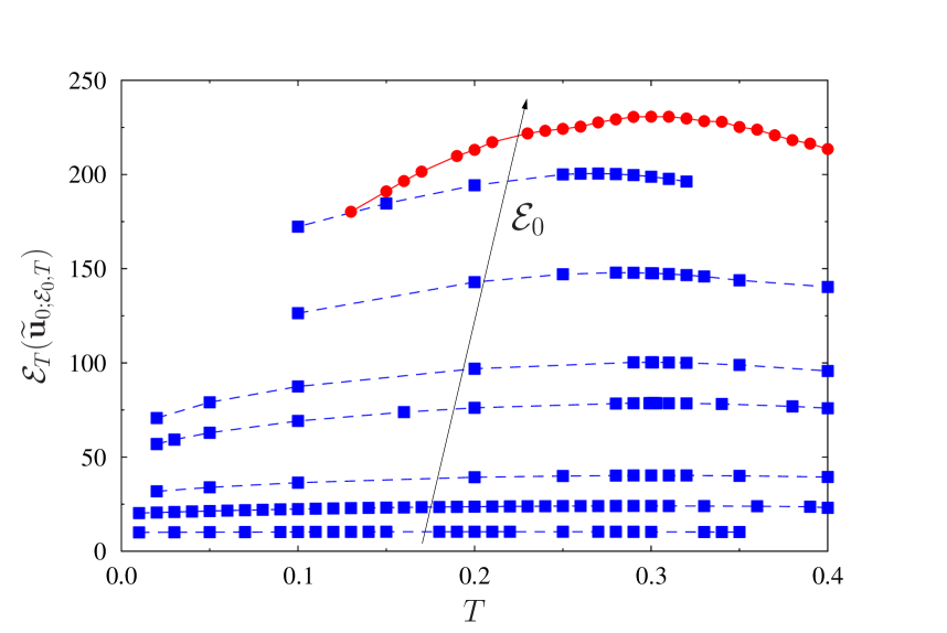
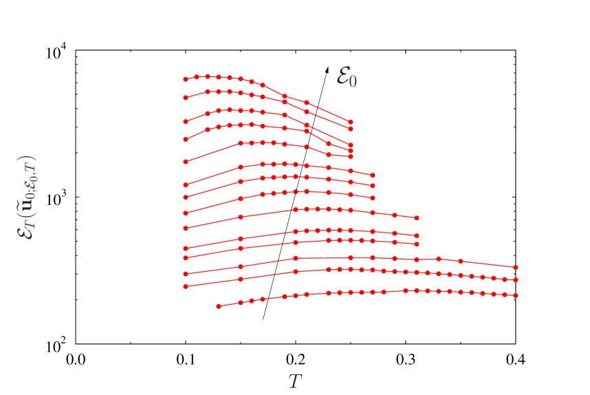
Figure 4: Maximum attained enstrophy ${\mathcal{E}}_{T}(\widetilde{\mathbf{u}}_{0;{\mathcal{E}}_{0},T})$ as a function of the length $T$ of the time interval over which maximization is performed in Problem 3.1 for initial enstrophies (a) $0<{\mathcal{E}}_{0}\leq 100$ and (b) $100<{\mathcal{E}}_{0}\leq 1000$. Blue dashed and red solid curves correspond to flow evolutions starting from, respectively, symmetric and asymmetric optimal initial conditions $\widetilde{\mathbf{u}}_{0;{\mathcal{E}}_{0},T}$ with the same value of the initial enstrophy and different $T$ (the trends with the increase of ${\mathcal{E}}_{0}$ are indicated with arrows, whereas solid symbols represent the values of ${\mathcal{E}}_{0}$ and $T$ for which Problem 3.1 was solved).

We thus have evidence for the existence of maximizers $\widetilde{\mathbf{u}}_{0;{\mathcal{E}}_{0},T}$ of two distinct types: those for which the flow evolution is characterized by the properties $\forall t\in[0,\widetilde{T}_{{\mathcal{E}}_{0}}]\quad{\mathcal{E}}_{1}({\mathbf{u}}(t))={\mathcal{E}}_{2}({\mathbf{u}}(t))={\mathcal{E}}_{3}({\mathbf{u}}(t))=(1/3){\mathcal{E}}({\mathbf{u}}(t))$ and ${\mathcal{H}}({\mathbf{u}}(t))=0$, and those for which these properties do not hold. We will refer to these families of maximizers as “symmetric” and “asymmetric”, respectively. The symmetric maximizers are normally found when the finite-time optimization problem 3.1 is solved for ${\mathcal{E}}_{0}<100$, whereas the asymmetric maximizers are found when this problem is solved for ${\mathcal{E}}_{0}>100$. However, maximizers of both types were found for ${\mathcal{E}}_{0}\approx 100$. These results are illustrated in figures 4(a) and 4(b) where we show the dependence of the maximum attained enstrophy ${\mathcal{E}}_{T}(\widetilde{\mathbf{u}}_{0;{\mathcal{E}}_{0},T})$ on the length $T$ of the time interval over which optimization was performed in Problem 3.1 for initial enstrophies ${\mathcal{E}}_{0}\leq 100$ and ${\mathcal{E}}>100$, respectively. In figure 4(a) we see that indeed two distinct branches of symmetric and asymmetric maximizers are simultaneously present when ${\mathcal{E}}_{0}=100$, thus demonstrating that these maximizers are nonunique. There are indications that symmetric maximizers also exist for ${\mathcal{E}}_{0}>100$ and asymmetric ones exist for ${\mathcal{E}}_{0}<100$, however, since they correspond to suboptimal local maxima, it is very difficult to compute them with the gradient approach (17). It is possible to capture both the symmetric and the asymmetric branch for ${\mathcal{E}}_{0}=100$, because for this value of the initial enstrophy the maximum attained enstrophy ${\mathcal{E}}_{T}(\widetilde{\mathbf{u}}_{0;{\mathcal{E}}_{0},T})$ is comparable for both branches. The asymmetry of optimal initial data $\widetilde{\mathbf{u}}_{0;{\mathcal{E}}_{0},T}$ on the asymmetric branch vanishes as $T\rightarrow 0.13$ which indicates that for ${\mathcal{E}}_{0}=100$ the asymmetric branch bifurcates off the symmetric branch at $T\approx 0.13$. In figure 4(b) a significant, albeit finite, increase of the enstrophy growth is observed as a function of ${\mathcal{E}}_{0}$ when asymmetric maximizers $\widetilde{\mathbf{u}}_{0;{\mathcal{E}}_{0},T}$ are used as the initial data for system (2) and this figure also confirms that for each value of the initial enstrophy ${\mathcal{E}}_{0}$ the maximum enstrophy ${\mathcal{E}}_{T}(\widetilde{\mathbf{u}}_{0;{\mathcal{E}}_{0},T})$ achieves a well-defined maximum for a certain optimal time $\widetilde{T}_{{\mathcal{E}}_{0}}$. We note that the accuracy with which $\widetilde{T}_{{\mathcal{E}}_{0}}$ can be determined for given ${\mathcal{E}}_{0}$ is limited by the number of time intervals $[0,T]$ for which the finite-time optimization problem 3.1 can be solved, which is a matter of the computational cost. However, we use spline interpolation to improve the accuracy with which the quantities $\max_{T>0}{\mathcal{E}}_{T}(\widetilde{\mathbf{u}}_{0;{\mathcal{E}}_{0},T})$ and $\widetilde{T}_{{\mathcal{E}}_{0}}$ are determined for a given initial enstrophy ${\mathcal{E}}_{0}$.

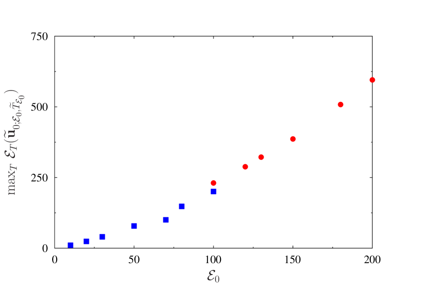
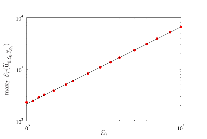
Figure 5: Dependence of the maximum enstrophy growth $\max_{T>0}\,{\mathcal{E}}_{T}(\widetilde{\mathbf{u}}_{0;{\mathcal{E}}_{0},T})$ on the initial enstrophy using (a) linear scaling for small ${\mathcal{E}}_{0}$ and (b) logarithmic scaling for large ${\mathcal{E}}_{0}$. The blue squares and red circles correspond to, respectively, the symmetric and asymmetric branches of solutions of the finite-time optimization problem 3.1 for different ${\mathcal{E}}_{0}$. The black solid line in panel (b) represents the least-squares fit (29).

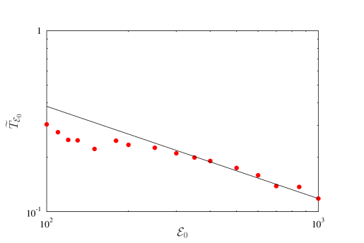
Figure 6: Dependence of the time $\widetilde{T}_{{\mathcal{E}}_{0}}$ when the maximum enstrophy $\max_{T>0}\,{\mathcal{E}}_{T}(\widetilde{\mathbf{u}}_{0;{\mathcal{E}}_{0},T})$ is achieved (with asymmetric maximizers) on the initial enstrophy ${\mathcal{E}}_{0}$. The red circles represent the interpolated data corresponding to solutions of the finite-time optimization problem 3.1 for different ${\mathcal{E}}_{0}$, whereas the black solid line represents the least-squares fit (30).

As the central result of this study, the maximum growth of enstrophy $\max_{T>0}{\mathcal{E}}_{T}(\widetilde{\mathbf{u}}_{0;{\mathcal{E}}_{0},T})$ achieved using initial conditions with enstrophy ${\mathcal{E}}_{0}$ is shown in figure 5 as a function of ${\mathcal{E}}_{0}$. In figure 5(a) corresponding to small values of ${\mathcal{E}}_{0}$ we see that the dependence of $\max_{T>0}{\mathcal{E}}_{T}(\widetilde{\mathbf{u}}_{0;{\mathcal{E}}_{0},T})$ on ${\mathcal{E}}_{0}$ appears slightly different for the symmetric and asymmetric branches, i.e., for ${\mathcal{E}}_{0}<100$ and ${\mathcal{E}}_{0}>100$. As is evident from figure 5(b), for asymmetric maximizers this growth follows a well-defined power-law relation

$$\max_{T>0}{\mathcal{E}}_{T}(\widetilde{\mathbf{u}}_{0;{\mathcal{E}}_{0},T})\ \sim\ \left(0.224\ \pm 0.006\right)\,{\mathcal{E}}_{0}^{1.490\,\pm 0.004}$$ (29)

obtained by performing a least-squares fit of the relation between $\log_{10}\left[\max_{T>0}{\mathcal{E}}_{T}(\widetilde{\mathbf{u}}_{0;{\mathcal{E}}_{0},T})\right]$ and $\log_{10}{\mathcal{E}}_{0}$ for $100\leq{\mathcal{E}}_{0}\leq 1000$. The fit is performed in the logarithmic coordinates in order for the least-squares error not to be dominated by contributions from the data corresponding to large values of ${\mathcal{E}}_{0}$. As regards the times when the maxima are achieved for different values of ${\mathcal{E}}_{0}$, when asymmetric maximizers are considered and the initial enstrophy is sufficiently large $({\mathcal{E}}_{0}\gtrapprox 400$), figure 6 shows that $\widetilde{T}_{{\mathcal{E}}_{0}}$ also exhibits a power-law dependence on ${\mathcal{E}}_{0}$, described by the relation

$$\widetilde{T}_{{\mathcal{E}}_{0}}\ \sim\ \left(4.0\,\pm 1.1\right)\,{\mathcal{E}}_{0}^{-0.51\,\pm 0.04}$$ (30)

obtained from a least-squares fit of the relation between ${\mathcal{E}}_{0}$ and $\widetilde{T}_{{\mathcal{E}}_{0}}$. We observe that for the maximum enstrophy $\max_{T>0}{\mathcal{E}}_{T}(\widetilde{\mathbf{u}}_{0;{\mathcal{E}}_{0},T})$ the power-law dependence on ${\mathcal{E}}_{0}$ becomes evident starting from smaller values of ${\mathcal{E}}_{0}$ and the fit is characterized by smaller error bars than for $\widetilde{T}_{{\mathcal{E}}_{0}}$, cf. figures 5(b) and 6. We also remark that the dependence of $\widetilde{T}_{{\mathcal{E}}_{0}}$ on ${\mathcal{E}}_{0}$ given in (30) appears different from the form of the upper bounds on the maximum blow-up time obtained by Ohkitani (2016). We add that the times $t_{0}$ when the upper bound in estimate (11) becomes unbounded are about 8–10 orders of magnitude shorter than the times $\widetilde{T}_{{\mathcal{E}}_{0}}$ shown in figure 6.

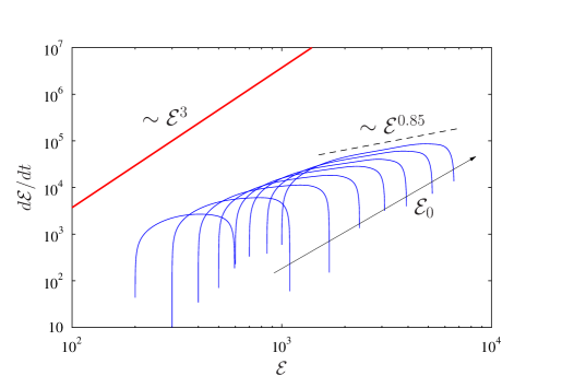
Figure 7: Flow trajectories corresponding to the optimal initial data $\widetilde{\mathbf{u}}_{0;{\mathcal{E}}_{0},\widetilde{T}_{{\mathcal{E}}_{0}}}$ with different ${\mathcal{E}}_{0}\in[100,1000]$, cf. figure 3(b–c), shown using the coordinates $\{{\mathcal{E}},d{\mathcal{E}}/dt\}$ (blue solid lines with the arrow indicating the trend with the increase of ${\mathcal{E}}_{0}$). The thick red line represents the relation $d{\mathcal{E}}/dt=1.72\cdot 10^{-3}\,{\mathcal{E}}^{3}$, cf. figure 1, whereas the dashed black line represents the relation $d{\mathcal{E}}/dt=10^{2}\,{\mathcal{E}}^{0.85}$.

In order to understand how close the flow evolutions corresponding to the optimal initial data $\widetilde{\mathbf{u}}_{0;{\mathcal{E}}_{0},\widetilde{T}_{{\mathcal{E}}_{0}}}$ come to saturating a priori bounds on the rate of growth of enstrophy, cf. (10), in figure 7 we plot the corresponding trajectories using the coordinates $\{{\mathcal{E}},d{\mathcal{E}}/dt\}$, such that each trajectory is parameterized by time $t$ (since the logarithmic scale is used, initial parts of the trajectories when $d{\mathcal{E}}/dt\lessapprox 0$ are not shown). The slope of the tangent to each of the curves thus represents the exponent $\alpha$ characterizing the instantaneous rate of enstrophy production $d{\mathcal{E}}/dt\sim{\mathcal{E}}^{\alpha}$. In figure 7 we also indicate the relation $d{\mathcal{E}}/dt=1.72\cdot 10^{-3}\,{\mathcal{E}}^{3}$ describing the maximum rate of enstrophy growth realized by the solutions of the instantaneous optimization problem 2.1 (Ayala & Protas, 2017), cf. figure 1 (we note that the prefactor in this relation is approximately 7 orders of magnitude smaller than the prefactor in estimate (10)). We observe that the rate of growth of enstrophy realized by the trajectories corresponding to the optimal initial conditions $\widetilde{\mathbf{u}}_{0;{\mathcal{E}}_{0},\widetilde{T}_{{\mathcal{E}}_{0}}}$ is at all times and for all values of ${\mathcal{E}}_{0}$ several orders of magnitude smaller than the maximum rate of growth achieved by the instantaneous maximizers $\widetilde{\mathbf{u}}_{{\mathcal{E}}_{0}}$, cf. figure 1. On the other hand, in figure 7 we also note that the exponent $\alpha$ characterizing the growth of enstrophy can be much larger than 3 at intermediate stages along these trajectories (we recall from the discussion in §2 that the rate of enstrophy production $d{\mathcal{E}}/dt\sim{\mathcal{E}}^{\alpha}$ must be sustained with $\alpha>2$ over a sufficiently long time interval for enstrophy to become unbounded in finite time). We add that at the final stages of the flow evolutions before the enstrophy maximum is reached at $t=\widetilde{T}_{{\mathcal{E}}_{0}}$ the enstrophy is amplified at the approximate rate $d{\mathcal{E}}/dt\sim{\mathcal{E}}^{0.85}$.

                   

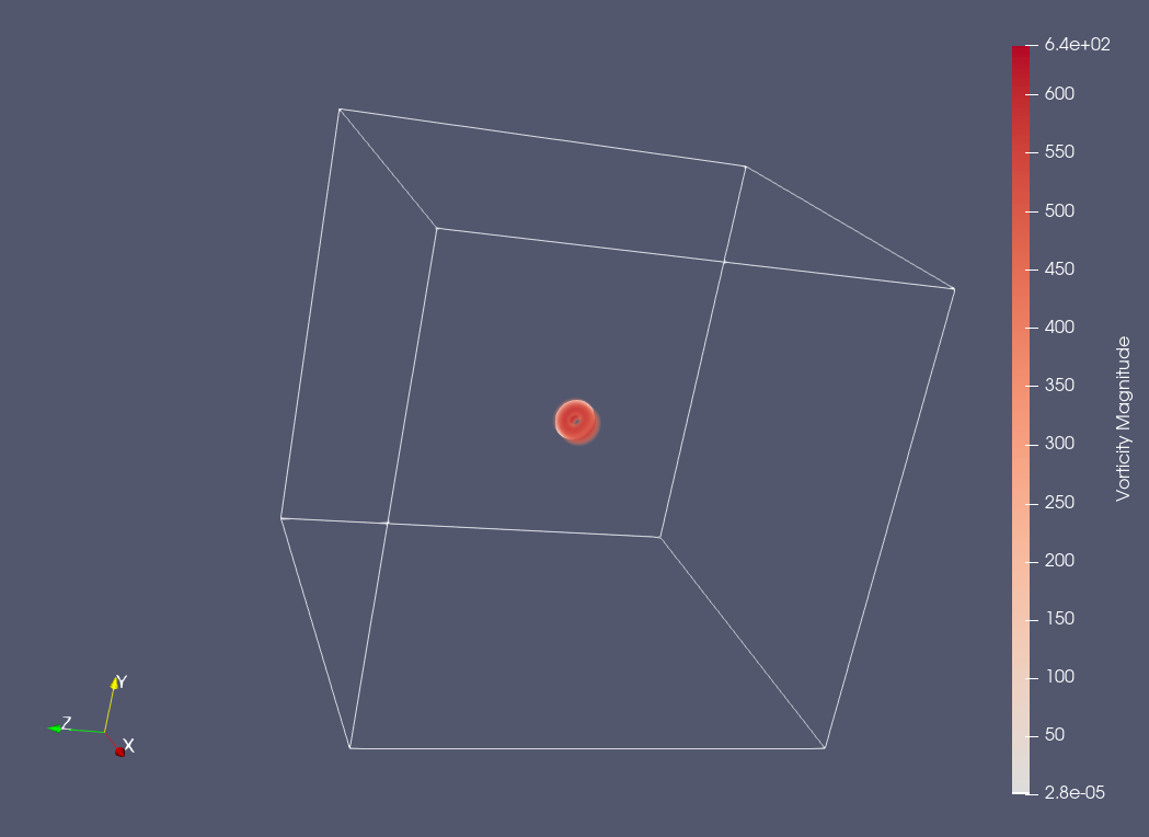
(a) instantaneous

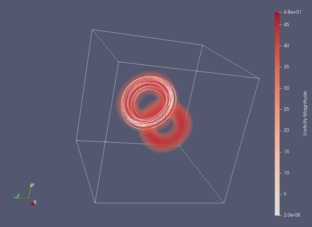
(b) $T=0.1$ (symmetric)

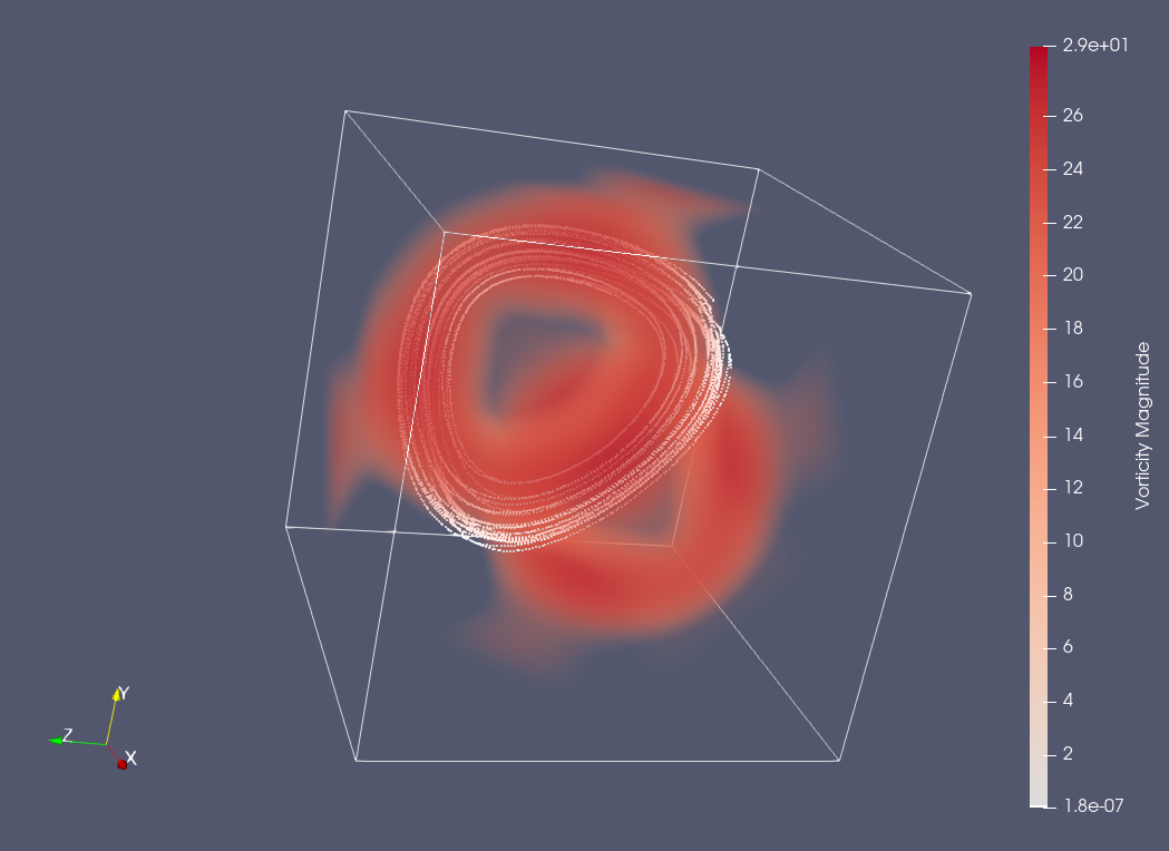
(c) $T=0.2$ (symmetric)

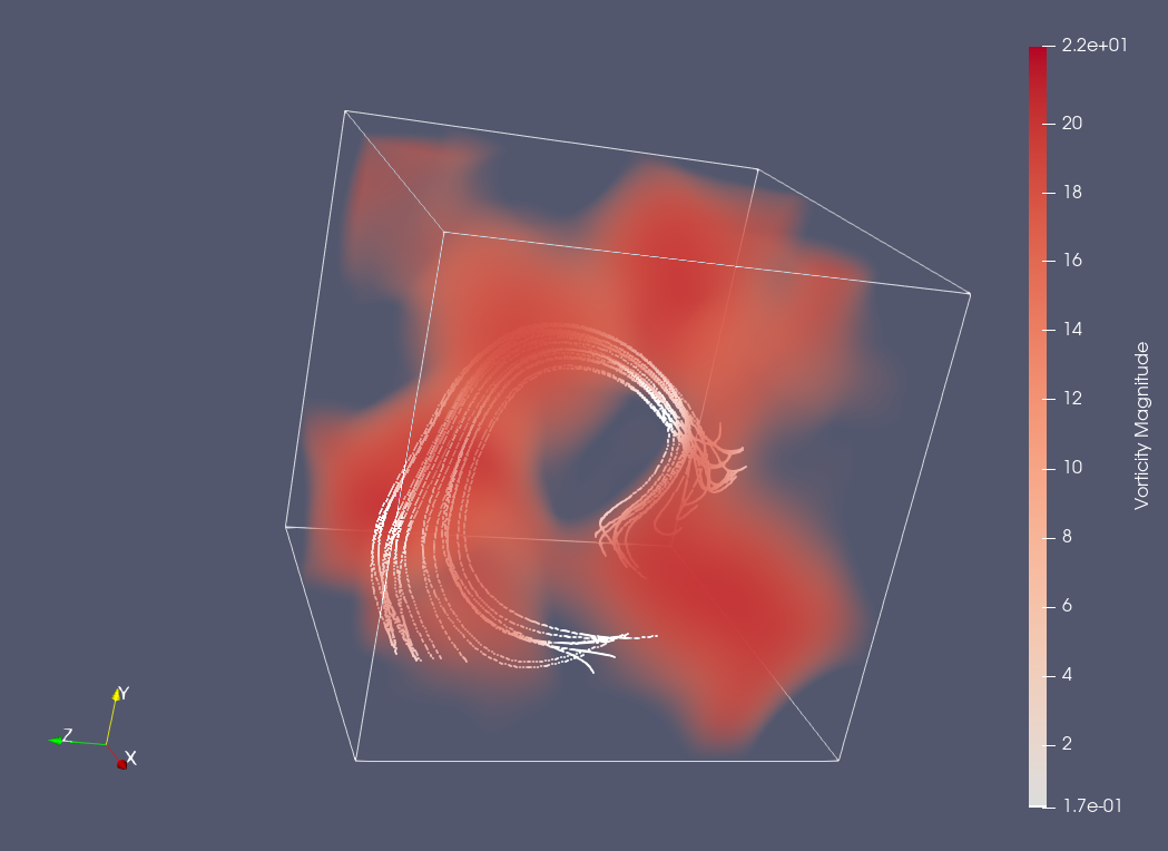
(d) $T=0.2$ (asymmetric)

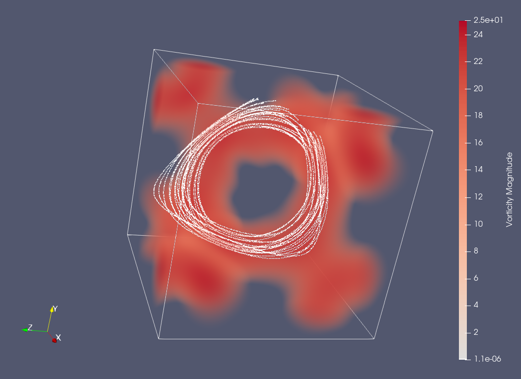
(e) $T=0.3$ (symmetric)

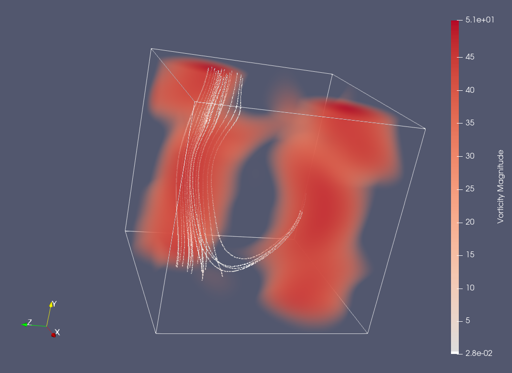
(f) $T=0.3=\widetilde{T}_{{\mathcal{E}}_{0}}$ (asymmetric)

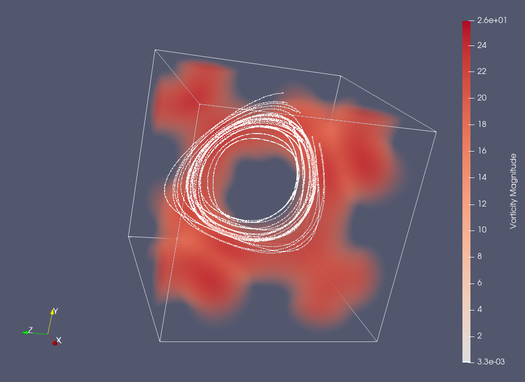
(g) $T=0.33$ (symmetric)

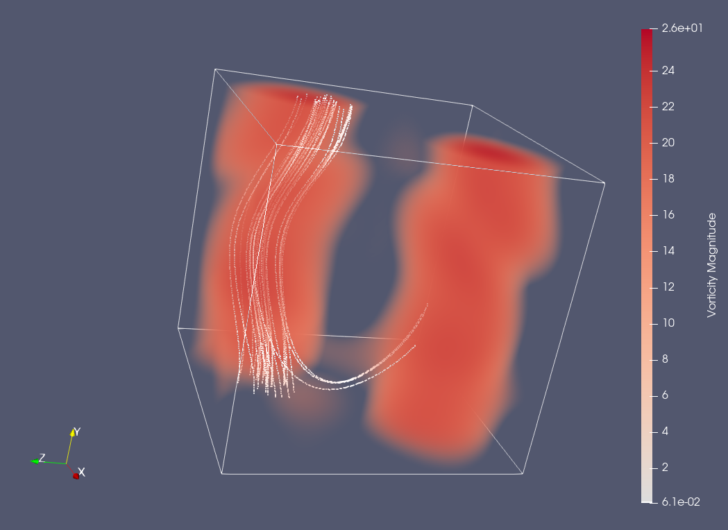
(h) $T=0.4$ (asymmetric)

Figure 8: Optimal initial conditions (a) $\widetilde{\mathbf{u}}_{{\mathcal{E}}_{0}}$ obtained by solving the instantaneous optimization problem 2.1 and (b–h) $\widetilde{\mathbf{u}}_{0;{\mathcal{E}}_{0},T}$ obtained by solving the finite-time optimization problem 3.1 for the initial enstrophy ${\mathcal{E}}_{0}=100$ and indicated lengths $T$ of the time interval. Optimal initial conditions from both the symmetric and asymmetric branch are shown. Shades of red correspond to the magnitude of the vorticity $|\left(\boldsymbol{\nabla}\times\widetilde{\mathbf{u}}_{{\mathcal{E}}_{0}}\right)({\mathbf{x}})|$ or $|\left(\boldsymbol{\nabla}\times\widetilde{\mathbf{u}}_{0;{\mathcal{E}}_{0},T}\right)({\mathbf{x}})|$ (see the color bars), whereas white curves represent vortex lines chosen to pass through regions with strong vorticity.

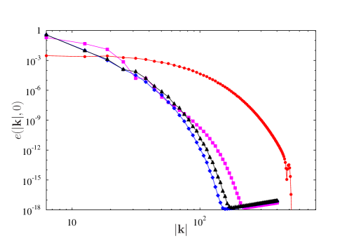
Figure 9: Energy spectra of the optimal initial conditions $\widetilde{\mathbf{u}}_{{\mathcal{E}}_{0}}$ and $\widetilde{\mathbf{u}}_{0;{\mathcal{E}}_{0},T}$ obtained by solving the instantaneous optimization problem 2.1 (red circles) and the finite-time optimization problem 3.1 for the initial enstrophy ${\mathcal{E}}_{0}=100$ and $T=0.1$ (pink squares), $T=0.2$ (blue diamonds) and $T=0.3$ (black triangles). In the latter case the optimal initial conditions $\widetilde{\mathbf{u}}_{0;{\mathcal{E}}_{0},T}$ come from the asymmetric branch.

We now move on to characterize the structure of the optimal initial conditions which give rise to the maximum enstrophy growth reported in figures 2, 4 and 5. First, in figure 8 we analyze the structure of both the symmetric and asymmetric initial conditions $\widetilde{\mathbf{u}}_{0;{\mathcal{E}}_{0},T}$ obtained by solving the finite-time optimization problem 3.1 for a fixed ${\mathcal{E}}_{0}=100$ and different $T$, and also show the instantaneously optimal initial condition $\widetilde{\mathbf{u}}_{{\mathcal{E}}_{0}}$ obtained as a solution of Problem 2.1 for the same value of ${\mathcal{E}}_{0}$ (Ayala & Protas, 2017). These initial conditions are presented in figure 8 in terms of their vorticity $\boldsymbol{\nabla}\times\widetilde{\mathbf{u}}_{0;{\mathcal{E}}_{0},T}$ and $\boldsymbol{\nabla}\times\widetilde{\mathbf{u}}_{{\mathcal{E}}_{0}}$, whose magnitude is visualized via volume rendering and, in addition, we also show a number of vortex lines (i.e., lines everywhere tangent to the vorticity field) chosen to pass through regions with strong vorticity. Such an approach allows us to simultaneously assess both the intensity and the structure of the vorticity field. In figure 8 we see that as $T$ increases the structure of the optimal initial condition gradually changes from two colliding vortex rings characterizing the instantaneous maximizers $\widetilde{\mathbf{u}}_{{\mathcal{E}}_{0}}$ (Lu & Doering, 2008; Ayala & Protas, 2017) to a more complex vorticity distribution filling the entire flow domain. There are also evident differences between the optimal initial conditions belonging to the symmetric and asymmetric branches, cf. figures 8(b,c,e,g) versus figures 8(d,f,h) — while the former retain the structure of deformed rings, the latter develop a tubular form. Since the asymmetric optimal initial conditions $\widetilde{\mathbf{u}}_{0;{\mathcal{E}}_{0},T}$ give rise to a much larger growth of enstrophy, cf. figure 5, hereafter we will exclusively focus on this case.

The fact that the optimal initial conditions $\widetilde{\mathbf{u}}_{0;{\mathcal{E}}_{0},T}$ obtained by solving the finite-time optimization problem 3.1 are less localized than the maximizers of the instantaneous optimization problem 2.1 is also evident from figure 9 showing their energy spectra $e(|{\mathbf{k}}|,0)$ defined as

$$e(|{\mathbf{k}}|,t):=\int_{S_{|{\mathbf{k}}|}}|{\mathbf{k}}|^{2}\left|\left[\widehat{{\mathbf{u}}}(t)\right]_{{\mathbf{k}}}\right|^{2}\,d\sigma,$$ (31)

where $\left[\widehat{{\mathbf{u}}}(t)\right]_{{\mathbf{k}}}$ are the Fourier coefficients of the velocity field ${\mathbf{u}}(t)$, $\sigma$ is the solid angle in the wavenumber space and $S_{|{\mathbf{k}}|}$ denotes the sphere of radius $|{\mathbf{k}}|$ in this space, such that ${\mathcal{K}}({\mathbf{u}}(t))=\int_{0}^{\infty}e(k,t)\,dk$ (with some abuse of notation justified by simplicity, here we have treated the wavevector ${\mathbf{k}}$ as a continuous rather than discrete variable). In figure 9 we see that while all the fields $\widetilde{\mathbf{u}}_{0;{\mathcal{E}}_{0},T}$ remain real-analytic (their energy spectra vanish exponentially fast for high wavenumbers $|{\mathbf{k}}|$), interestingly, the ones corresponding to intermediate lengths $T\approx 0.2$ of the optimization interval are in fact the smoothest in the sense that their energy spectra $e(|{\mathbf{k}}|,0)$ decay fastest with $|{\mathbf{k}}|$. In particular, the energy spectrum of the instantaneously optimal initial condition $\widetilde{\mathbf{u}}_{{\mathcal{E}}_{0}}$ decays much slower. These observations indicate that the finite-time optimization problems 3.1 corresponding to intermediate and longer time intervals $T$ are in fact less demanding in terms of space resolution $N$, which is why for larger values of the initial enstrophy ${\mathcal{E}}_{0}$ it is easier to perform continuation with respect to ${\mathcal{E}}_{0}$ at some fixed intermediate $T$, rather than the other way round starting from the instantaneous maximizers $\widetilde{\mathbf{u}}_{{\mathcal{E}}_{0}}$ which are hard to compute when ${\mathcal{E}}_{0}>100$.

              

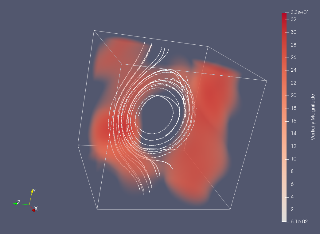
(a) ${\mathcal{E}}_{0}=150$, $\widetilde{T}_{{\mathcal{E}}_{0}}=0.27$

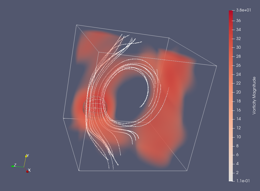
(b) ${\mathcal{E}}_{0}=200$, $\widetilde{T}_{{\mathcal{E}}_{0}}=0.23$

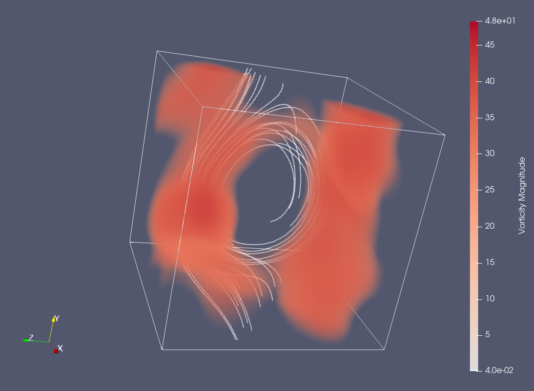
(c) ${\mathcal{E}}_{0}=300$, $\widetilde{T}_{{\mathcal{E}}_{0}}=0.21$

(d) ${\mathcal{E}}_{0}=400$, $\widetilde{T}_{{\mathcal{E}}_{0}}=0.19$

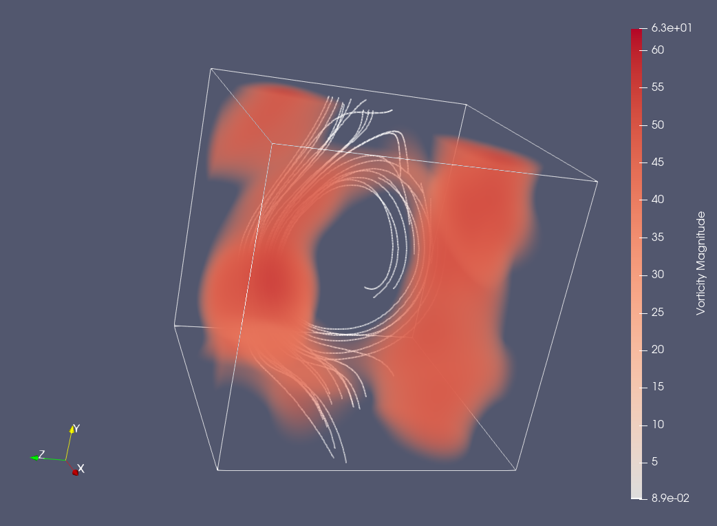
(e) ${\mathcal{E}}_{0}=500$, $\widetilde{T}_{{\mathcal{E}}_{0}}=0.17$

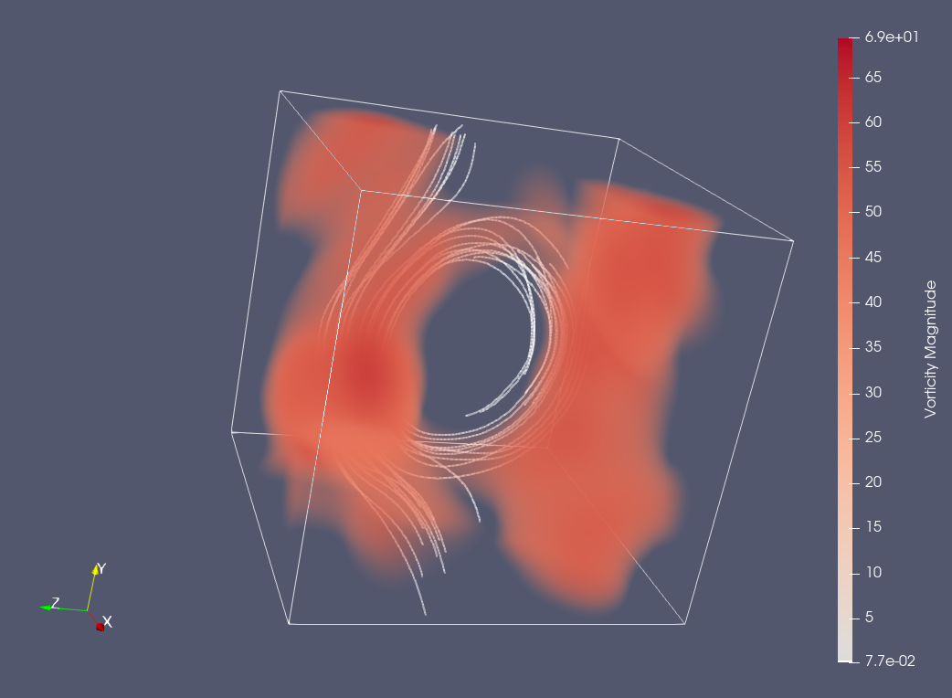
(f) ${\mathcal{E}}_{0}=600$, $\widetilde{T}_{{\mathcal{E}}_{0}}=0.15$

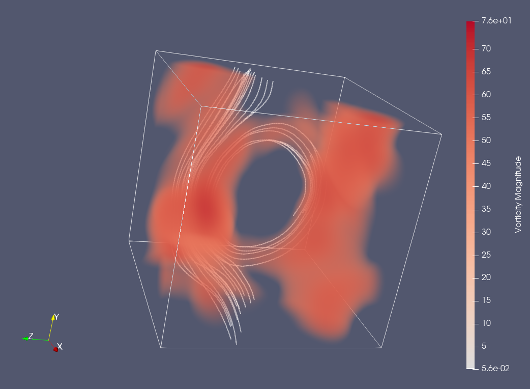
(g) ${\mathcal{E}}_{0}=700$, $\widetilde{T}_{{\mathcal{E}}_{0}}=0.14$

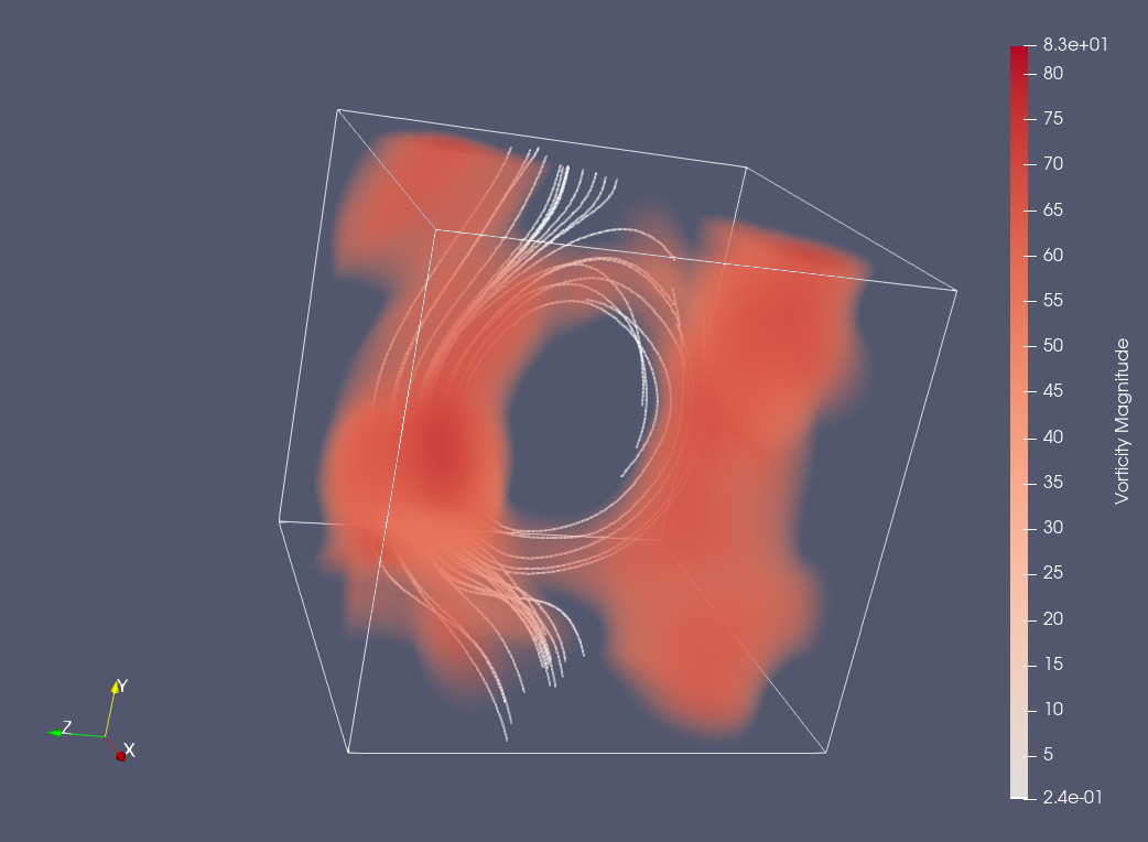
(h) ${\mathcal{E}}_{0}=850$, $\widetilde{T}_{{\mathcal{E}}_{0}}=0.13$

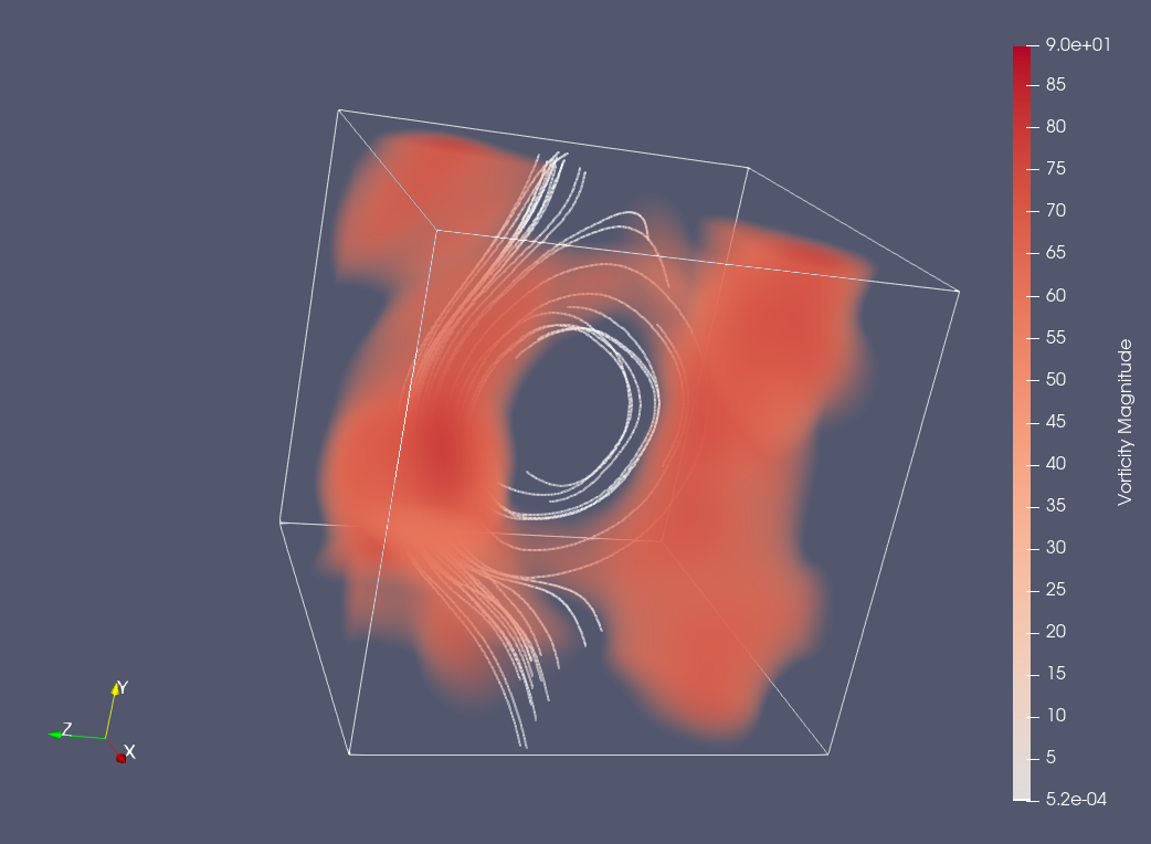
(i) ${\mathcal{E}}_{0}=1000$, $\widetilde{T}_{{\mathcal{E}}_{0}}=0.12$

Figure 10: Asymmetric optimal initial conditions $\widetilde{\mathbf{u}}_{0;{\mathcal{E}}_{0},\widetilde{T}_{{\mathcal{E}}_{0}}}$ obtained by solving the finite-time optimization problem 3.1 for different indicated values of the initial enstrophy ${\mathcal{E}}_{0}$ and the corresponding optimal lengths $\widetilde{T}_{{\mathcal{E}}_{0}}$ of the time interval (cf. figure 6). Shades of red correspond to the magnitude of the vorticity $\left|\left(\boldsymbol{\nabla}\times\widetilde{\mathbf{u}}_{0;{\mathcal{E}}_{0},\widetilde{T}_{{\mathcal{E}}_{0}}}\right)({\mathbf{x}})\right|$ (see the color bars), whereas white curves represent vortex lines chosen to pass through regions with strong vorticity.

    

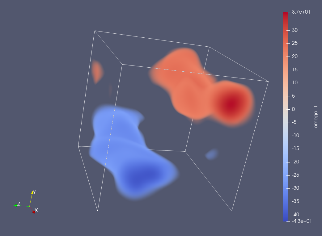
(a) $\widetilde{\omega}_{1}$

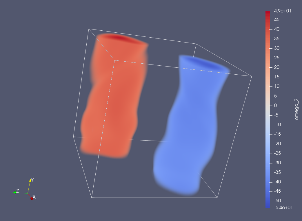
(b) $\widetilde{\omega}_{2}$

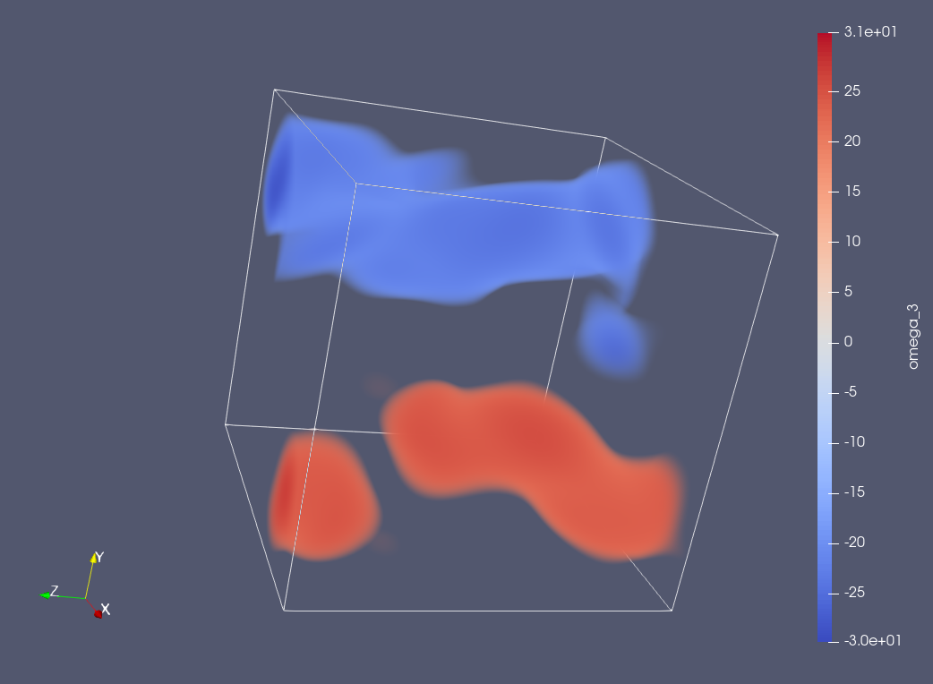
(c) $\widetilde{\omega}_{3}$

Figure 11: Vorticity components of the asymmetric optimal initial condition $\widetilde{\mathbf{u}}_{0;{\mathcal{E}}_{0},\widetilde{T}_{{\mathcal{E}}_{0}}}$ obtained by solving the finite-time optimization problem 3.1 for the initial enstrophy ${\mathcal{E}}_{0}=500$ and the corresponding optimal length $\widetilde{T}_{{\mathcal{E}}_{0}}=0.17$ of the time interval, cf. figure 10(e).

The optimal asymmetric initial conditions $\widetilde{\mathbf{u}}_{0;{\mathcal{E}}_{0},\widetilde{T}_{{\mathcal{E}}_{0}}}$ obtained for the optimal time intervals $[0,\widetilde{T}_{{\mathcal{E}}_{0}}]$ are shown in figure 10 for increasing values of the initial enstrophy ${\mathcal{E}}_{0}$. We note that the structure of these fields does not much change with ${\mathcal{E}}_{0}$, except that, as expected, the vorticity magnitude $\left|\left(\boldsymbol{\nabla}\times\widetilde{\mathbf{u}}_{0;{\mathcal{E}}_{0},\widetilde{T}_{{\mathcal{E}}_{0}}}\right)({\mathbf{x}})\right|$ in the vortex regions increases. In order to shed additional light on the structure of these optimal initial conditions, the field $\widetilde{\mathbf{u}}_{0;{\mathcal{E}}_{0},\widetilde{T}_{{\mathcal{E}}_{0}}}$ corresponding to the initial enstrophy ${\mathcal{E}}_{0}=500$, cf. figure 10(e), is further analyzed in figure 11 in terms of its different vorticity components $[\widetilde{\omega}_{1}(t),\widetilde{\omega}_{2}(t),\widetilde{\omega}_{3}(t)]^{T}:=\boldsymbol{\nabla}\times{\mathbf{u}}(t)$. We observe that the optimal initial condition has in fact the form of three perpendicular pairs of anti-parallel vortex tubes perturbed near the regions where they intersect (these perturbations allow the vorticity field to satisfy the divergence-free condition $\boldsymbol{\nabla}\cdot\left(\boldsymbol{\nabla}\times\widetilde{\mathbf{u}}_{0;{\mathcal{E}}_{0},\widetilde{T}_{{\mathcal{E}}_{0}}}\right)=0$). The relative magnitudes of the three vorticity components are given by the approximate relations $0.76\,:\,1\,:\,0.63$ representing the ratios $\widetilde{\omega}_{1}\,:\;\widetilde{\omega}_{2}\,:\,\widetilde{\omega}_{3}$.

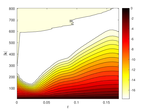
Figure 12: Time evolution of the energy spectrum in the solution of the Navier-Stokes system (2) with the optimal asymmetric initial condition $\widetilde{\mathbf{u}}_{0;{\mathcal{E}}_{0},T}$ obtained by solving the the finite-time optimization problem 3.1 for the initial enstrophy ${\mathcal{E}}_{0}=500$ and $\widetilde{T}_{{\mathcal{E}}_{0}}=0.17$. The contour lines represent the level sets of the function $\log_{10}e(|{\mathbf{k}}|,t)$ with the distance between two nearby lines corresponding to one order of magnitude.

Next, we analyze details of the flow evolution corresponding to the optimal initial conditions $\widetilde{\mathbf{u}}_{0;{\mathcal{E}}_{0},T}$. In figure 12 we illustrate the evolution of the energy spectrum $e(|{\mathbf{k}}|,t)$, cf. (31), in time in the solution of the Navier-Stokes system (2) with the optimal asymmetric initial condition $\widetilde{\mathbf{u}}_{0;{\mathcal{E}}_{0},T}$ obtained by solving the the finite-time optimization problem 3.1 with ${\mathcal{E}}_{0}=500$ and $\widetilde{T}_{{\mathcal{E}}_{0}}=0.17$, cf. figure 11 (qualitatively similar behavior is also observed for other values of ${\mathcal{E}}_{0}>100$). We notice that at early stages of the flow evolution the energy spectrum recedes which corresponds to the initially very slow growth of enstrophy already noted in figure 2. Then, the energy begins to flow towards larger wavenumbers such that the energy spectrum becomes the most developed close to the final time $t=\widetilde{T}_{{\mathcal{E}}_{0}}$ when the enstrophy maximum is achieved. As regards this second stage, there are clearly two phases ending at instances of time corresponding approximately to the times when the ordering of ${\mathcal{E}}_{1}({\mathbf{u}}(t))$, ${\mathcal{E}}_{2}({\mathbf{u}}(t))$ and ${\mathcal{E}}_{3}({\mathbf{u}}(t))$ changes, cf. figure 3(c). This indicates that there are in fact two reconnection events occurring during the flow evolution: one approximately in the middle of the time interval $[0,\widetilde{T}_{{\mathcal{E}}_{0}}]$ and another one close to its end.

        

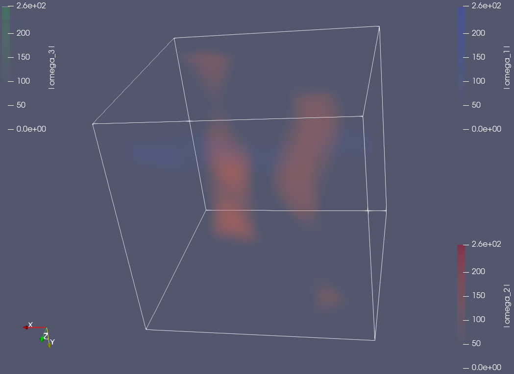
(a) $t=0.0$

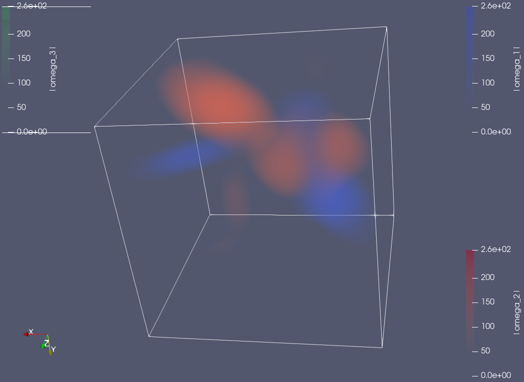
(b) $t=0.04$

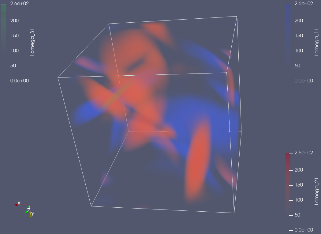
(c) $t=0.09$

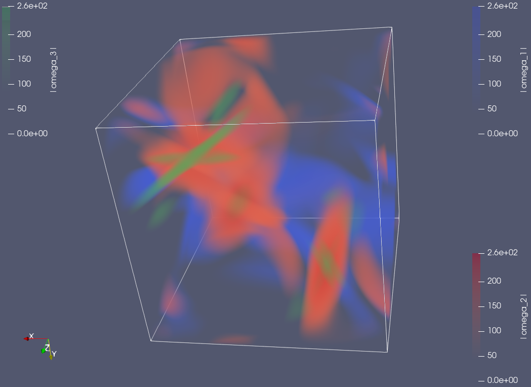
(d) $t=0.11$

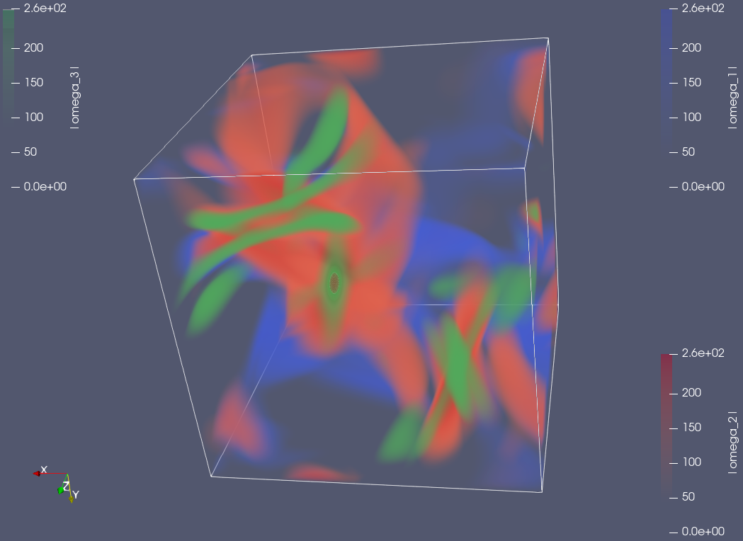
(e) $t=0.14$

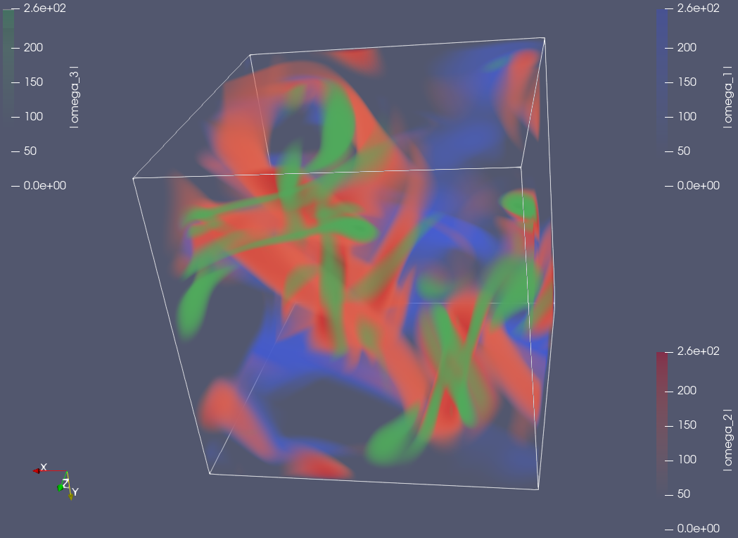
(f) $t=0.17=\widetilde{T}_{{\mathcal{E}}_{0}}$

Figure 13: Vorticity components (blue) $\widetilde{\omega}_{1}$, (red) $\widetilde{\omega}_{2}$ and (green) $\widetilde{\omega}_{3}$ at the indicated time instances in the solution of the Navier-Stokes system (2) with the optimal asymmetric initial condition $\widetilde{\mathbf{u}}_{0;{\mathcal{E}}_{0},T}$ obtained by solving the finite-time optimization problem 3.1 for the initial enstrophy ${\mathcal{E}}_{0}=500$ and $\widetilde{T}_{{\mathcal{E}}_{0}}=0.17$. Supporting Movie 1 is available on-line.

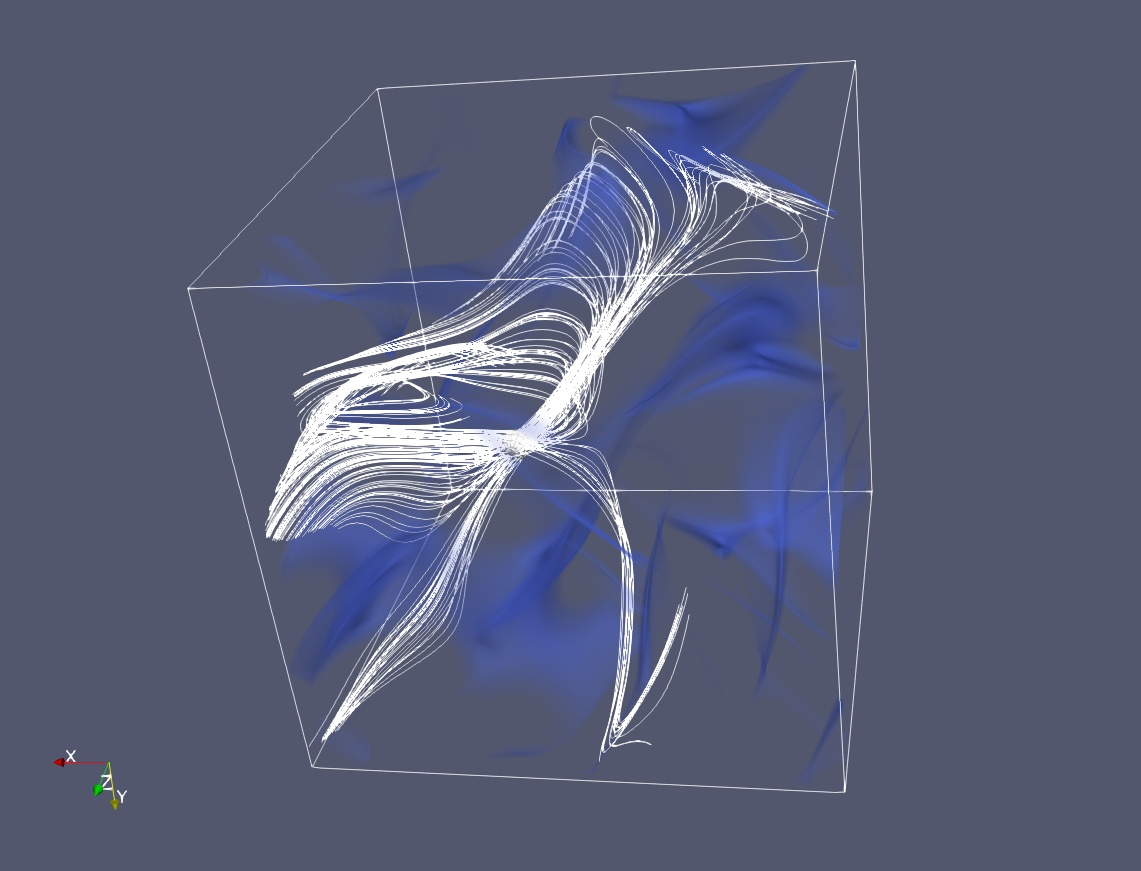
Figure 14: Reconnection event occurring at the time $t=0.09$ in the solution of the Navier-Stokes system (2) with the optimal initial conditions $\widetilde{\mathbf{u}}_{0;{\mathcal{E}}_{0},T}$ obtained by solving the finite-time optimization problem 3.1 for ${\mathcal{E}}_{0}=500$ and $\widetilde{T}_{{\mathcal{E}}_{0}}=0.17$, cf. figure 13(c). White lines represent the vortex lines in the neighborhood of the reconnection point whereas the blue regions correspond to locations where $|(\boldsymbol{\nabla}\times{\mathbf{u}})({\mathbf{x}})|\approx 0$.

Finally, we discuss the flow evolution in the physical space and the three vorticity components $\widetilde{\omega}_{1}$, $\widetilde{\omega}_{2}$ and $\widetilde{\omega}_{3}$ are shown in figure 13 at various times $t\in[0,\widetilde{T}_{{\mathcal{E}}_{0}}]$. Since the same color scale is used in all panels in this figure, some features of the optimal initial condition $\widetilde{\mathbf{u}}_{0;{\mathcal{E}}_{0},T}$ evident in figure 11 are not visible in figure 13(a). In agreement with figure 12, we observe that at the early stages of the flow evolution the vorticity field becomes less localized, cf. figure 13(b), which is followed by a rapid development of small scales, cf. figures 13(d,e). The final state $\boldsymbol{\nabla}\times{\mathbf{u}}(\widetilde{T}_{{\mathcal{E}}_{0}})$ is characterized by a fairly complicated structure with turbulent-like spatial complexity, cf. figure 13(f). In particular, it features a combination of tube-shaped and pancake-shaped regions of concentrated vorticity (animations corresponding to the vorticity fields shown in figure 13 and to optimal flow evolutions obtained for other values of ${\mathcal{E}}_{0}$ and $\widetilde{T}_{{\mathcal{E}}_{0}}$ are available on-line as Movies 1, 2 and 3). To provide more insight into what drives this flow evolution, in figure 14 we illustrate a typical reconnection event occurring approximately at the time when the ordering of ${\mathcal{E}}_{1}({\mathbf{u}}(t))$, ${\mathcal{E}}_{2}({\mathbf{u}}(t))$ and ${\mathcal{E}}_{3}({\mathbf{u}}(t))$ changes, cf. figures 3(c) and 13(c). We see that the bundle of vortex lines aligned with the direction $x_{2}$ and visible in the middle of the figure is split into two parts going in opposite directions, one of which attaches to a perpendicular bundle of vortex lines. In figure 14 we also visualize regions where $|(\boldsymbol{\nabla}\times{\mathbf{u}})({\mathbf{x}})|\approx 0$, which is a necessary condition for vortex reconnection to occur (Hussain & Duraisamy, 2011; Jaque & Fuentes, 2017). These regions are therefore potential loci of other reconnection events.

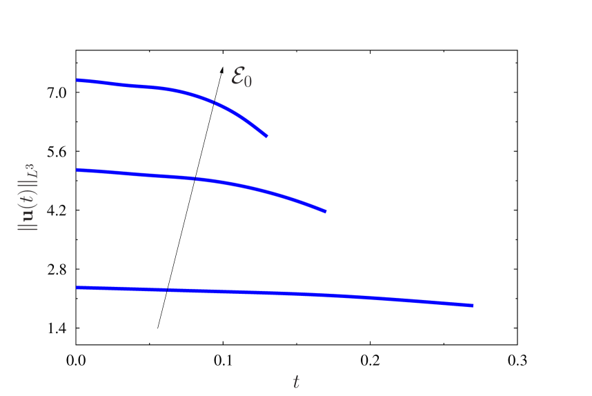
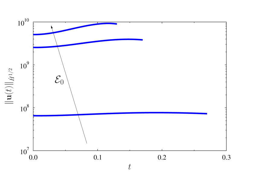
Figure 15: Evolution of (a) the norm $\|{\mathbf{u}}(t)\|_{L^{3}}$ and (b) the seminorm $\|{\mathbf{u}}(t)\|_{\dot{H}^{1/2}}$ of the solutions of the Navier-Stokes system (2) with the optimal asymmetric initial conditions $\widetilde{\mathbf{u}}_{0;{\mathcal{E}}_{0},T}$ obtained by solving the finite-time optimization problem 3.1 for ${\mathcal{E}}_{0}=100$ and $\widetilde{T}_{{\mathcal{E}}_{0}}=0.27$, ${\mathcal{E}}_{0}=500$ and $\widetilde{T}_{{\mathcal{E}}_{0}}=0.17$ and ${\mathcal{E}}_{0}=1000$ and $\widetilde{T}_{{\mathcal{E}}_{0}}=0.13$. Arrows indicates the trends with the increase of ${\mathcal{E}}_{0}$.

To close this section, in figure 15 we analyze the time evolution of the $L^{3}$ norm and the $H^{1/2}$ seminorm of the solutions of the Navier-Stokes system (2) with the optimal asymmetric initial conditions $\widetilde{\mathbf{u}}_{0;{\mathcal{E}}_{0},T}$ obtained by solving the finite-time optimization problem 3.1 for ${\mathcal{E}}_{0}=100,500,1000$ and with the corresponding optimal optimization time intervals $\widetilde{T}_{{\mathcal{E}}_{0}}$. These quantities, defined as

$$\|{\mathbf{u}}(t)\|_{L^{3}} :=\left(\int_{\Omega}|{\mathbf{u}}(t,{\mathbf{x}})|^{3}\,d{\mathbf{x}}\right)^{1/3},$$ (32a)

$${\|{\mathbf{u}}(t)\|_{\dot{H}^{1/2}}} :={\left[\sum_{{\mathbf{k}}\in{\mathbb{Z}}^{3}}|{\mathbf{k}}|\left|\left[\widehat{{\mathbf{u}}}(t)\right]_{{\mathbf{k}}}\right|^{2}\right]^{1/2}}$$ (32b)

are important, because they are critical norms in the analysis of the Navier-Stokes system (2) (Robinson et al., 2016). As we can see in figure 15(a), the $L^{3}$ norm decays monotonically in each case. On the other hand, the $H^{1/2}$ seminorm exhibits a significant transient growth, cf. figure 15(b), and, interestingly, its maxima are in each case achieved at intermediate times $0<t<\widetilde{T}_{{\mathcal{E}}_{0}}$, i.e., before the enstrophy maximum is attained at $\widetilde{T}_{{\mathcal{E}}_{0}}$.

Movie 1. (available on-line) Time evolution of the vorticity components (blue) $\widetilde{\omega}_{1}$, (red) $\widetilde{\omega}_{2}$ and (green) $\widetilde{\omega}_{3}$ in the solution of the Navier-Stokes system (2) with the optimal asymmetric initial condition $\widetilde{\mathbf{u}}_{0;{\mathcal{E}}_{0},T}$ obtained by solving the finite-time optimization problem 3.1 for the initial enstrophy ${\mathcal{E}}_{0}=500$ and $\widetilde{T}_{{\mathcal{E}}_{0}}=0.17$, cf. figure 13. The animation covers the time interval $[0,\widetilde{T}_{{\mathcal{E}}_{0}}]$.

Movie 2. (available on-line) Time evolution of the vorticity components (blue) $\widetilde{\omega}_{1}$, (red) $\widetilde{\omega}_{2}$ and (green) $\widetilde{\omega}_{3}$ in the solution of the Navier-Stokes system (2) with the optimal asymmetric initial condition $\widetilde{\mathbf{u}}_{0;{\mathcal{E}}_{0},T}$ obtained by solving the finite-time optimization problem 3.1 for the initial enstrophy ${\mathcal{E}}_{0}=300$ and $\widetilde{T}_{{\mathcal{E}}_{0}}=0.21$. The animation covers the time interval $[0,\widetilde{T}_{{\mathcal{E}}_{0}}]$.

Movie 3. (available on-line) Time evolution of the vorticity components (blue) $\widetilde{\omega}_{1}$, (red) $\widetilde{\omega}_{2}$ and (green) $\widetilde{\omega}_{3}$ in the solution of the Navier-Stokes system (2) with the optimal asymmetric initial condition $\widetilde{\mathbf{u}}_{0;{\mathcal{E}}_{0},T}$ obtained by solving the finite-time optimization problem 3.1 for the initial enstrophy ${\mathcal{E}}_{0}=1000$ and $\widetilde{T}_{{\mathcal{E}}_{0}}=0.12$. The animation covers the time interval $[0,\widetilde{T}_{{\mathcal{E}}_{0}}]$.

6 Discussion and Conclusions

In this study we have considered the question of the largest possible growth of enstrophy in finite time in 3D Navier-Stokes flows starting from initial data with enstrophy ${\mathcal{E}}_{0}$. This problem is motivated by the open question concerning the global-in-time existence of classical (smooth) solutions of the 3D Navier-Stokes system (Doering, 2009). One of the landmark results in this context is the conditional regularity result due to Foias & Temam (1989) asserting that solutions to the Navier-Stokes system (2) remain smooth and satisfy this system in the classical sense as long as the enstrophy remains finite. To probe this condition we have considered a family of optimization problems for the Navier-Stokes system (2), cf. Problem 3.1, in which initial data ${\mathbf{u}}_{0}$ with prescribed enstrophy ${\mathcal{E}}_{0}$ is sought such that the enstrophy at the given time $T$ is maximized. Thus, in each case the problem is solved on a fixed time domain and there are two parameters, ${\mathcal{E}}_{0}$ and $T$. For each value of ${\mathcal{E}}_{0}$ the optimal time window $\widetilde{T}_{{\mathcal{E}}_{0}}$ is then determined by solving problem 3.1 for several different values of $T$, cf. figure 4. In principle, this last step could be eliminated by finding the optimal time window $\widetilde{T}_{{\mathcal{E}}_{0}}$ as a part of the solution of a suitably modified optimization problem 3.1 in which the final enstrophy would be simultaneously maximized with respect to the initial condition ${\mathbf{u}}_{0}$ and the length $T$ of the time window. However, such a modified optimization problem would then be of the free-boundary type, because its time domain $[0,T]$ would not be a priori known, leading to significant complications in its numerical solution. Therefore, it is preferable to solve Problem 3.1 for different values of the two parameters ${\mathcal{E}}_{0}$ and $T$, which is facilitated by the continuation approach. For given values of ${\mathcal{E}}_{0}$ and $T$, Problem 3.1 is solved computationally with a state-of-the-art adjoint-based gradient ascent technique. Our approach is formulated in the continuous (“optimize-then-discretize”) setting with gradients defined in a suitable Sobolev space, cf. (18) and (25), which allows us to ensure that the optimal initial conditions possess the required minimum regularity. The governing and adjoint systems, (2) and (22), are solved efficiently with a massively parallel pseudo-spectral approach. Being based on the first-order optimality conditions, this gradient optimization approach makes it possible to find local maximizers only and it is not possible to guarantee that these maximizers are global. In order to partially address this issue, in addition to the continuation approach described in $3, cf. Algorithm 1, we have also undertaken an extensive search for other maximizing branches using suitably randomized initial guesses ${\mathbf{u}}^{0}$ in (17) which however did not yield any maximizers distinct from the two branches, a symmetric and an asymmetric one, already reported in §5. Nevertheless, the existence of other branches of maximizers cannot be ruled out.

For every considered value of the initial enstrophy ${\mathcal{E}}_{0}$ on both the symmetric and asymmetric branch there exists a well-defined time $\widetilde{T}_{{\mathcal{E}}_{0}}$ such that the optimized growth of the enstrophy at this time is maximal. The structure of the optimal initial condition producing this growth is quite different on the symmetric and the asymmetric branch, and changes as the initial enstrophy increases, cf. figure 10. In the limit of large ${\mathcal{E}}_{0}$ the asymmetric branch dominates in terms of the maximum enstrophy growth and the corresponding initial conditions have the form of three perpendicular pairs of anti-parallel vortex tubes, cf. figure 11. Thus, our subsequent analysis has focused on this family of initial data. Interestingly, as is evident from figure 9, these optimal initial conditions $\widetilde{\mathbf{u}}_{0;{\mathcal{E}}_{0},T}$ are smoother than the solutions $\widetilde{\mathbf{u}}_{{\mathcal{E}}_{0}}$ of the instantaneous optimization optimization problem 2.1 obtained for the same value of ${\mathcal{E}}_{0}$ (to be precise, the velocity fields are real-analytic in both cases, but in the latter case the energy spectra decay at a slower, though still exponential, rate). Consequently, solution of the finite-time optimization problem 3.1 requires a lower numerical resolution than the corresponding instantaneous problem 2.1 and, as a result, we have been able to solve the finite-time problem for values of the initial enstrophy ${\mathcal{E}}_{0}$ an order of magnitude higher than it was possible for the instantaneous maximization problem in Ayala & Protas (2017). Further on this note, we also observe that the extremal flow trajectories originating from the optimal initial conditions $\widetilde{\mathbf{u}}_{0;{\mathcal{E}}_{0},T}$ involve velocity fields which become even smoother at early stages of their evolution, cf. figures 12 and 13, before developing small-scale components at later stages when the maximum enstrophy is achieved. In other words, in these optimal flow evolutions the energy flux is initially from small to large scales, and then in the opposite direction near the end of the optimization interval $[0,\widetilde{T}_{{\mathcal{E}}_{0}}]$. This behavior can be understood by considering system (8) from which it is evident that large enstrophy implies rapid energy dissipation. At the same time it is known that a 3D Navier-Stokes flow may not generate significant enstrophy unless its energy is sufficiently large (Ayala & Protas, 2017). Thus, in order to maximize its enstrophy at some large time $T$, an optimal flow seeks to reduce its production at early stages in order to conserve energy while rearranging itself strategically such that a sequence of bursts of energy to small scales will produce maximum enstrophy at the final time $T$.

The main finding of the present study is that the worst-case enstrophy-maximizing Navier-Stokes flow evolutions constructed by solving a suitable optimization problem always lead to a finite only growth of enstrophy. This suggests that unbounded growth of enstrophy allowed by estimate (11) cannot, in fact, be realized and, in the light of the conditional regularity result (1), even under the extremal flow evolution there is no evidence for singularity formation in finite time. This also suggests the possibility of improving estimate (11) with the power-law relation (29) serving as a potential target. As a matter of course, the validity of these findings is restricted by the possibility that we may not have found true global maximizers of Problem 3.1. To be more specific, the maximum enstrophy produced in flows with initial data with enstrophy ${\mathcal{E}}_{0}$ was found to scale in proportion to ${\mathcal{E}}_{0}^{3/2}$, cf. (29), which is the same power-law relation as observed by Ayala & Protas (2011) in solutions of an analogous finite-time optimization problem for the 1D Burgers equation. This scaling can be in fact predicted based on dimensional analysis. Noting that the largest flow structures have characteristic dimension comparable to the size of the domain $L$, cf. figures 10 and 13, there are three physical parameters defining the problem, namely, ${\mathcal{E}}_{0}$, $L$ and the kinematic viscosity $\nu$. The only nontrivial way to combine them gives ${\mathcal{E}}_{T}\sim\left(L/\nu^{2}\right)^{1/2}{\mathcal{E}}_{0}^{3/2}$. In addition, we can deduce that $T\sim L^{3/2}{\mathcal{E}}_{0}^{-1/2}$ which represents the scaling for $\widetilde{T}_{{\mathcal{E}}_{0}}$ observed in figure 6, cf. (30). In this context it would be interesting to know what form the optimal initial conditions would take if Problem 3.1 were solved on an unbounded domain $\Omega={\mathbb{R}}^{3}$. Since for a fixed initial enstrophy ${\mathcal{E}}_{0}$ the optimal initial conditions discussed in §5 would vanish in the limit $L\rightarrow\infty$, the solutions of this problem would likely have a completely different form. We add that in the instantaneous optimization problem in which the characteristic dimension of the flow structures does not scale with $L$, dimensional analysis also correctly predicts that $d{\mathcal{E}}/dt\sim{\mathcal{E}}^{3}/\nu^{3}$, cf. (10) (Lu & Doering, 2008).

Two distinct branches of maximizing initial conditions were found with the one consisting of asymmetric states dominating in terms of the maximum growth of enstrophy in the limit of large ${\mathcal{E}}_{0}$. The corresponding initial conditions have the form of three perpendicular pairs of anti-parallel vortex tubes and the flow evolution resulting from this initial data is quite complex, cf. figure 13, involving an initial flux of energy from small to large scales followed by a sequence of reconnection events, cf. figure 14. At its final stages the flow evolution has the spatio-temporal complexity of turbulent flows, although there is no evidence of a Kolmogorov-type -5/3 energy spectrum in figure 9. This can be explained by the fact that we consider an initial-value problem for system (2) and no statistically steady state is attained during the evolution. More work is still needed to understand in detail the physical mechanisms responsible for the extreme flow evolutions illustrated in figure 13, for example, in terms of changes of the topology of vortex lines. In particular, the fact that helicity remains zero during all flow evolutions starting from the optimal initial conditions $\widetilde{\mathbf{u}}_{0;{\mathcal{E}}_{0},\widetilde{T}_{{\mathcal{E}}_{0}}}$ implies the presence of some symmetries in the velocity field. We add that no evidence for reconnection was found in the flow evolutions starting from the optimal initial conditions on the symmetric branch.

In involving pairs of anti-parallel vortex tubes the optimal initial conditions $\widetilde{\mathbf{u}}_{0;{\mathcal{E}}_{0},\widetilde{T}_{{\mathcal{E}}_{0}}}$ we found resemble the configurations investigated in several earlier studies of extreme flow behavior (Melander & Hussain, 1989; Kerr, 1993, 2013a, 2013b, 2018). In particular, Orlandi et al. (2012) used two perpendicular pairs of anti-parallel vortex tubes (referred to as “dipoles” in that study). Although in the case of Navier-Stokes flows none of these studies showed evidence of singularity formation in finite time, they all reported various forms of viscous vortex reconnection. More precisely, while the enstrophy would increase during the reconnection events, it would in all cases remain bounded. Based on three values of the Reynolds number defined as $Re:=\left({\mathcal{K}}({\mathbf{u}}_{0})\,{\mathcal{E}}_{0}\right)^{1/4}/\nu$, the results reported by Orlandi et al. (2012) exhibit a linear dependence of the maximum attained enstrophy on the Reynolds number, i.e., $\max_{t}{\mathcal{E}}(t)\sim Re$. For comparison, noting that in our case ${\mathcal{K}}(\widetilde{\mathbf{u}}_{0;{\mathcal{E}}_{0},\widetilde{T}_{{\mathcal{E}}_{0}}})\sim{\mathcal{E}}_{0}$ and therefore $Re\sim{\mathcal{E}}_{0}^{1/2}$, the power-law relation (29) takes the form $\max_{T>0}{\mathcal{E}}_{T}(\widetilde{\mathbf{u}}_{0;{\mathcal{E}}_{0},T})\sim Re^{3}$ when expressed in terms of the Reynolds number defined above. Thus, even though the range of the Reynolds numbers explored in our study was approximately two orders of magnitude lower than in Orlandi et al. (2012), in the flows studied here the maximum attained enstrophy grows much more rapidly when the Reynolds number is increased. We add that the “trefoil” initial condition which recently received attention (Kerr, 2018) is in fact fundamentally different from the optimal initial data studied here, because it is meant to be defined on an unbounded, rather than periodic, domain. Moreover, unlike the optimal initial conditions $\widetilde{\mathbf{u}}_{0;{\mathcal{E}}_{0},\widetilde{T}_{{\mathcal{E}}_{0}}}$ and the corresponding flows, it is characterized by nonzero helicity.

Our results indicate that even in the worst-case scenario the nonlinear mechanisms of vortex stretching are significantly depleted, This observation is consistent with the findings of Donzis et al. (2013); Gibbon et al. (2014) who studied the behavior of suitably-scaled higher-order Lebesgue norms of vorticity in a number of different numerical simulations of turbulent Navier-Stokes flows, both forced and decaying. They provided evidence for a significant depletion of the rate of growth of enstrophy as compared to (9). More precisely, they demonstrated that in their simulations enstrophy amplification tends to occur at the rate $d{\mathcal{E}}/dt\sim{\mathcal{E}}^{\alpha}$ with $\alpha\in[1.575,1.75]$ (we recall from our discussion in §2 that $\alpha<2$ implies a regular behavior of the flow). These findings are also consistent with our observations, cf. figure 7, indicting that while in the flow evolutions corresponding to the optimal initial data $\widetilde{\mathbf{u}}_{0;{\mathcal{E}}_{0},\widetilde{T}_{{\mathcal{E}}_{0}}}$ the enstrophy may occasionally be amplified at the much higher rate, the sustained rate is proportional to ${\mathcal{E}}^{\alpha}$ with $0<\alpha<2$.

The results summarized above represent a final stage of the research program outlined in Table 1 which aimed to characterize the largest possible growth of enstrophy and enstrophy-like quantities in 1D Burgers and 2D & 3D Navier-Stokes flows. In particular, we sought to understand whether the sharpest estimates on the growth of these quantities obtained using energy-type methods can be realized in actual flows. Somewhat paradoxically, the situation concerning 1D Burgers flows, where the best finite-time estimate obtained using energy methods was found not to be sharp (Ayala & Protas, 2011), is less satisfactory than in the case of 2D Navier-Stokes flows where the estimates for both the instantaneous and finite-time growth of palinstrophy were shown to be sharp (and, interestingly, they are realized by the same field (Ayala & Protas, 2014a; Ayala et al., 2018)). Moving forward, a natural next step is to consider other conditional regularity results complementary to condition (1). More specifically, we will probe the family of the Ladyzhenskaya-Prodi-Serrin conditions asserting that Navier-Stokes flows ${\mathbf{u}}(t)$ are smooth and satisfy system (2) in the classical sense provided that (Kiselev & Ladyzhenskaya, 1957; Prodi, 1959; Serrin, 1962)

$${\mathbf{u}}\in L^{p}([0,T];L^{q}(\Omega)),\quad 2/p+3/q\leq 1,\quad q>3.$$ (33)

These conditions were recently generalized by Gibbon (2018) to include norms of the derivatives of the velocity field. The main technical difficulty in testing conditions (33) is that some of the corresponding variational optimization problems will be formulated on function spaces without the Hilbert structure and will therefore require more specialized approaches (Protas, 2008). Moreover, some of these optimization problems may also be nonsmooth. In addition, there are questions concerning potential finite-time singularity formation in inviscid Euler flows which can also be framed in terms of the extreme growth of enstrophy-like quantities. We intend to investigate both these questions in the near future.

References

- Adams & Fournier (2005) Adams, R. A. & Fournier, J. F. 2005 Sobolev Spaces. Elsevier.
- Ayala (2014) Ayala, D. 2014 Extreme Vortex States and Singularity Formation in Incompressible Flows. PhD thesis, McMaster University, available at http://hdl.handle.net/11375/15453.
- Ayala et al. (2018) Ayala, Diego, Doering, Charles R. & Simon, Thilo M. 2018 Maximum palinstrophy amplification in the two-dimensional Navier-Stokes equations. Journal of Fluid Mechanics 837, 839–857.
- Ayala & Protas (2011) Ayala, D. & Protas, B. 2011 On maximum enstrophy growth in a hydrodynamic system. Physica D 240, 1553–1563.
- Ayala & Protas (2014a) Ayala, D. & Protas, B. 2014a Maximum palinstrophy growth in 2D incompressible flows. Journal of Fluid Mechanics 742, 340–367.
- Ayala & Protas (2014b) Ayala, D. & Protas, B. 2014b Vortices, maximum growth and the problem of finite-time singularity formation. Fluid Dynamics Research 46 (3), 031404.
- Ayala & Protas (2017) Ayala, D. & Protas, B. 2017 Extreme vortex states and the growth of enstrophy in 3D incompressible flows. Journal of Fluid Mechanics 818, 772–806.
- Beale et al. (1984) Beale, J. T., Kato, T. & Majda, A. 1984 Remarks on the breakdown of smooth solutions for the -D Euler equations. Comm. Math. Phys. 94 (1), 61–66.
- Berger (1977) Berger, M. S. 1977 Nonlinearity and Functional Analysis. Academic Press.
- Bewley (2009) Bewley, T. R. 2009 Numerical Renaissance. Renaissance Press.
- Biryuk (2001) Biryuk, A. È. 2001 Spectral properties of solutions of the burgers equation with small dissipation. Functional Analysis and Its Applications 35 (1), 1–12.
- Brachet (1991) Brachet, M. E. 1991 Direct simulation of three-dimensional turbulence in the Taylor-Green vortex. Fluid Dynamics Research 8, 1–8.
- Brachet et al. (1983) Brachet, M. E., Meiron, D. I., Orszag, S. A., Nickel, B. G., Morf, R. H. & Frisch, U. 1983 Small-scale structure of the Taylor-Green vortex. Journal of Fluid Mechanics 130, 411–452.
- Bustamante & Brachet (2012) Bustamante, M. D. & Brachet, M. 2012 Interplay between the Beale-Kato-Majda theorem and the analyticity-strip method to investigate numerically the incompressible Euler singularity problem. Phys. Rev. E 86, 066302.
- Bustamante & Kerr (2008) Bustamante, M. D. & Kerr, R. M. 2008 3D Euler about a 2D symmetry plane. Physica D 237, 1912–1920.
- Caffarelli et al. (1982) Caffarelli, L., Kohn, R. & Nirenberg, L. 1982 Partial regularity of suitable weak solutions of the navier-stokes equations. Communications on Pure and Applied Mathematics 35 (6), 771–831.
- Campolina & Mailybaev (2018) Campolina, Ciro S. & Mailybaev, Alexei A. 2018 Chaotic blowup in the 3d incompressible euler equations on a logarithmic lattice. Phys. Rev. Lett. 121, 064501.
- Chernyshenko et al. (2014) Chernyshenko, S. I., Goulart, P., Huang, D. & Papachristodoulou, A. 2014 Polynomial sum of squares in fluid dynamics: a review with a look ahead. Philosophical Transactions of the Royal Society A: Mathematical, Physical and Engineering Sciences 372 (2020), 20130350.
- Davidson (2004) Davidson, P. A. 2004 Turbulence. An introduction for scientists and engineers. Oxford University Press.
- Doering (2009) Doering, C. R. 2009 The 3D Navier-Stokes problem. Annual Review of Fluid Mechanics 41, 109–128.
- Doering & Constantin (1992) Doering, Charles R. & Constantin, Peter 1992 Energy dissipation in shear driven turbulence. Phys. Rev. Lett. 69, 1648–1651.
- Doering & Gibbon (1995) Doering, C. R. & Gibbon, J. D. 1995 Applied Analysis of the Navier-Stokes Equations. Cambridge University Press.
- Donzis et al. (2013) Donzis, Diego A., Gibbon, John D., Gupta, Anupam, Kerr, Robert M., Pandit, Rahul & Vincenzi, Dario 2013 Vorticity moments in four numerical simulations of the 3D Navier-Stokes equations. Journal of Fluid Mechanics 732, 316–331.
- Elgindi & Jeong (2018) Elgindi, Tarek M. & Jeong, In-Jee 2018 Finite-time Singularity formation for Strong Solutions to the axi-symmetric 3D Euler Equations. ArXiv:1802.09936.
- Fantuzzi & Goluskin (2019) Fantuzzi, Giovanni & Goluskin, David 2019 Bounding extreme events in nonlinear dynamics using convex optimization. ArXiv:1907.10997.
- Fefferman (2000) Fefferman, C. L. 2000 Existence and smoothness of the Navier-Stokes equation. available at http://www.claymath.org/sites/default/files/navierstokes.pdf, Clay Millennium Prize Problem Description.
- Feng & Šverák (2015) Feng, Hao & Šverák, Vladimír 2015 On the cauchy problem for axi-symmetric vortex rings. Archive for Rational Mechanics and Analysis 215 (1), 89–123.
- Foias & Temam (1989) Foias, C. & Temam, R. 1989 Gevrey class regularity for the solutions of the Navier–Stokes equations. Journal of Functional Analysis 87, 359–369.
- Frigo & Johnson (2003) Frigo, Matteo & Johnson, Steven G. 2003 FFTW User’s Manual. Massachusetts Institute of Technology.
- Gibbon et al. (2014) Gibbon, J.D, Donzis, D., Gupta, A., Kerr, R.M., Pandit, R. & Vincenzi, D. 2014 Regimes of nonlinear depletion and regularity in the 3D Navier-Stokes equations. Nonlinearity 27 (1–19).
- Gibbon (2018) Gibbon, J. D. 2018 Weak and Strong Solutions of the 3D Navier–Stokes Equations and Their Relation to a Chessboard of Convergent Inverse Length Scales. Journal of Nonlinear Science (published on-line).
- Gibbon et al. (2008) Gibbon, J. D., Bustamante, M. & Kerr, R. M. 2008 The three–dimensional Euler equations: singular or non–singular? Nonlinearity 21, 123–129.
- Goluskin (2018) Goluskin, David 2018 Bounding Averages Rigorously Using Semidefinite Programming: Mean Moments of the Lorenz System. Journal of Nonlinear Science 28 (2), 621–651.
- Goluskin & Fantuzzi (2019) Goluskin, David & Fantuzzi, Giovanni 2019 Bounds on mean energy in the Kuramoto–Sivashinsky equation computed using semidefinite programming. Nonlinearity 32 (5), 1705–1730.
- Grafke et al. (2008) Grafke, T., Homann, H., Dreher, J. & Grauer, R. 2008 Numerical simulations of possible finite-time singularities in the incompressible Euler equations: comparison of numerical methods. Physica D 237, 1932–1936.
- Gunzburger (2003) Gunzburger, M. D. 2003 Perspectives in Flow Control and Optimization. SIAM.
- Hou (2009) Hou, T. Y. 2009 Blow-up or no blow-up? a unified computational and analytic approach to 3D incompressible Euler and Navier–Stokes equations. Acta Numerica pp. 277–346.
- Hou & Li (2007) Hou, T. Y. & Li, R. 2007 Computing nearly singular solutions using pseudo-spectral methods. Journal of Computational Physics 226, 379–397.
- Hussain & Duraisamy (2011) Hussain, Fazle & Duraisamy, Karthik 2011 Mechanics of viscous vortex reconnection. Physics of Fluids 23 (2), 021701.
- Jaque & Fuentes (2017) Jaque, Ruben Suaza & Fuentes, Oscar Velasco 2017 Reconnection of orthogonal cylindrical vortices. European Journal of Mechanics - B/Fluids 62, 51 – 56.
- Kerr (1993) Kerr, R. M. 1993 Evidence for a singularity of the three-dimensional, incompressible Euler equations. Phys. Fluids A 5, 1725–1746.
- Kerr (2013a) Kerr, R. M. 2013a Bounds for Euler from vorticity moments and line divergence. Journal of Fluid Mechanics 729, R2.
- Kerr (2013b) Kerr, Robert M. 2013b Swirling, turbulent vortex rings formed from a chain reaction of reconnection events. Physics of Fluids 25, 065101.
- Kerr (2018) Kerr, Robert M. 2018 Enstrophy and circulation scaling for Navier-Stokes reconnection. Journal of Fluid Mechanics 839, R2.
- Kiselev (2010) Kiselev, A. 2010 Regularity and blow up for active scalars. Math. Model. Nat. Phenom. 5, 225–255.
- Kiselev et al. (2008) Kiselev, A., Nazaraov, F. & Shterenberg, R. 2008 Blow up and regularity for fractal Burgers equation. Dynamics of Partial Differential Equations 5, 211–240.
- Kiselev & Ladyzhenskaya (1957) Kiselev, A. A. & Ladyzhenskaya, O. A. 1957 On the existence and uniqueness of the solution of the nonstationary problem for a viscous, incompressible fluid. Izv. Akad. Nauk SSSR Ser. Mat 21 (5), 655–680.
- Kreiss & Lorenz (2004) Kreiss, H. & Lorenz, J. 2004 Initial-Boundary Value Problems and the Navier-Stokes Equations, Classics in Applied Mathematics, vol. 47. SIAM.
- Leray (1934) Leray, Jean 1934 Sur le mouvement d’un liquide visqu’eux emplissant l’espace. Acta Mathematica 63 (1), 193–248.
- Lu (2006) Lu, L. 2006 Bounds on the enstrophy growth rate for solutions of the 3D Navier-Stokes equations. PhD thesis, University of Michigan.
- Lu & Doering (2008) Lu, L. & Doering, C. R. 2008 Limits on enstrophy growth for solutions of the three-dimensional Navier–Stokes equations. Indiana University Mathematics Journal 57, 2693–2727.
- Luenberger (1969) Luenberger, D. 1969 Optimization by Vector Space Methods. John Wiley and Sons.
- Luo & Hou (2014a) Luo, G. & Hou, T. Y. 2014a Potentially Singular Solutions of the 3D Axisymmetric Euler Equations. Proceedings of the National Academy of Sciences 111 (36), 12968–12973.
- Luo & Hou (2014b) Luo, G. & Hou, T. Y. 2014b Toward the Finite-Time Blowup of the 3D Incompressible Euler Equations: a Numerical Investigation. SIAM: Multiscale Modeling and Simulation 12 (4), 1722–1776.
- Matsumoto et al. (2008) Matsumoto, T., Bec, J. & Frisch, U. 2008 Complex-space singularities of 2D Euler flow in lagrangian coordinates. Physica D 237, 1951–1955.
- Melander & Hussain (1989) Melander, M. V. & Hussain, F. 1989 Cross-linking of two antiparallel vortex tubes. Physics of Fluids A: Fluid Dynamics 1 (4), 633–636.
- Miller (2019) Miller, Evan 2019 A Regularity Criterion for the Navier-Stokes Equation Involving Only the Middle Eigenvalue of the Strain Tensor. Arch Rational Mech Anal .
- Moffatt & Kimura (2019a) Moffatt, H. K. & Kimura, Yoshifumi 2019a Towards a finite-time singularity of the Navier-Stokes equations Part 1. Derivation and analysis of dynamical system. Journal of Fluid Mechanics 861, 930–967.
- Moffatt & Kimura (2019b) Moffatt, H. K. & Kimura, Yoshifumi 2019b Towards a finite-time singularity of the Navier-Stokes equations. part 2. vortex reconnection and singularity evasion. Journal of Fluid Mechanics 870, R1.
- Nocedal & Wright (1999) Nocedal, J. & Wright, S. J. 1999 Numerical Optimization. Springer.
- Ohkitani (2008) Ohkitani, K. 2008 A miscellany of basic issues on incompressible fluid equations. Nonlinearity 21, 255–271.
- Ohkitani (2016) Ohkitani, Koji 2016 Late formation of singularities in solutions to the navier–stokes equations. Journal of Physics A: Mathematical and Theoretical 49 (1), 015502.
- Ohkitani & Constantin (2008) Ohkitani, K. & Constantin, P. 2008 Numerical study of the Eulerian–Lagrangian analysis of the Navier-Stokes turbulence. Phys. Fluids 20, 1–11.
- Orlandi et al. (2014) Orlandi, P., Pirozzoli, S., Bernardini, M. & Carnevale, G. F. 2014 A minimal flow unit for the study of turbulence with passive scalars. Journal of Turbulence 15, 731–751.
- Orlandi et al. (2012) Orlandi, P., Pirozzoli, S. & Carnevale, G. F. 2012 Vortex events in Euler and Navier-Stokes simulations with smooth initial conditions. Journal of Fluid Mechanics 690, 288–320.
- Pelinovsky (2012) Pelinovsky, D. 2012 Sharp bounds on enstrophy growth in the viscous Burgers equation. Proceedings of Royal Society A 468, 3636–3648.
- Pelz (2001) Pelz, R. B. 2001 Symmetry and the hydrodynamic blow-up problem. Journal of Fluid Mechanics 444, 299–320.
- Poças & Protas (2018) Poças, Diogo & Protas, Bartosz 2018 Transient growth in stochastic Burgers flows. Discrete & Continuous Dynamical Systems — B 23, 2371.
- Press et al. (1986) Press, W. H., Flannery, B. P., Teukolsky, S. A. & Vetterling, W. T. 1986 Numerical Recipes. Cambridge University Press.
- Prodi (1959) Prodi, Giovanni 1959 Un teorema di unicità per le equazioni di Navier-Stokes. Annali di Matematica Pura ed Applicata 48 (1), 173–182.
- Protas (2008) Protas, B. 2008 Adjoint-based optimization of PDE systems with alternative gradients. Journal of Computational Physics 227, 6490–6510.
- Protas et al. (2004) Protas, B., Bewley, T. & Hagen, G. 2004 A comprehensive framework for the regularization of adjoint analysis in multiscale PDE systems. Journal of Computational Physics 195, 49–89.
- Pumir & Siggia (1990) Pumir, A. & Siggia, E. 1990 Collapsing solutions to the 3D Euler equations. Phys. Fluids A 2, 220–241.
- Robinson et al. (2016) Robinson, James C., Rodrigo, José L. & Sadowski, Witold 2016 The Three-Dimensional Navier-Stokes Equations: Classical Theory. Cambridge University Press.
- Schumacher et al. (2010) Schumacher, Jörg, Eckhardt, Bruno & Doering, Charles R. 2010 Extreme vorticity growth in navier-stokes turbulence. Physics Letters A 374 (6), 861–865.
- Serrin (1962) Serrin, James 1962 On the interior regularity of weak solutions of the Navier-Stokes equations. Archive for Rational Mechanics and Analysis 9 (1), 187–195.
- Siegel & Caflisch (2009) Siegel, M. & Caflisch, R. E. 2009 Calculation of complex singular solutions to the 3D incompressible Euler equations. Physica D 238, 2368–2379.
- Tao (2016) Tao, Terence 2016 Finite time blowup for an averaged three-dimensional Navier-Stokes equation. J. Amer. Math. 29, 601–674.
- Tobasco et al. (2018) Tobasco, Ian, Goluskin, David & Doering, Charles R. 2018 Optimal bounds and extremal trajectories for time averages in nonlinear dynamical systems. Physics Letters A 382 (6), 382 – 386.
- Yun & Protas (2018) Yun, Dongfang & Protas, Bartosz 2018 Maximum Rate of Growth of Enstrophy in Solutions of the Fractional Burgers Equation. Journal of Nonlinear Science 28 (1), 395–422.