August 2019

MIT-CTP-5139

Hyperbolic String Vertices

Kevin Costello¹ and Barton Zwiebach²

¹ Perimeter Institute of Theoretical Physics,
31 Caroline St N, Waterloo, ON N2L 2Y5, Canada

² Center for Theoretical Physics,
Massachusetts Institute of Technology
Cambridge, MA 02139, USA

Abstract

The string vertices of closed string field theory are subsets of the moduli spaces of punctured Riemann surfaces that satisfy a geometric version of the Batalin-Vilkovisky master equation. We present a homological proof of existence of string vertices and their uniqueness up to canonical transformations. Using hyperbolic metrics on surfaces with geodesic boundaries we give an exact construction of string vertices as sets of surfaces with systole greater than or equal to $L$ with $L\leq 2\,\hbox{arcsinh}\,1$. Intrinsic hyperbolic collars prevent the appearance of short geodesics upon sewing. The surfaces generated by Feynman diagrams are naturally endowed with Thurston metrics: hyperbolic on the vertices and flat on the propagators. For the classical theory the length $L$ is arbitrary and, as $L\to\infty$ hyperbolic vertices become the minimal-area vertices of closed string theory.

1 Introduction

The key geometric input for the construction of string field theories is a set of string vertices. For the case of closed string field theories, including heterotic and type II strings, string vertices ${\cal V}_{g,n}$ are subsets of the moduli spaces of compact Riemann surfaces of genus $g$ and $n$ marked points, with a choice of local coordinates (defined up to phases) at those marked points. At genus zero string vertices are required for $n\geq 3$, at genus one for $n\geq 1$, and for genus two or greater, for $n\geq 0$. If consistent string vertices are known, a choice of a suitable conformal field theory allows the construction of bosonic closed string field theory[1]. With a choice of suitable superconformal field theories, a proper set of string fields, and careful distributions of picture changing operators, it is now known how to use string vertices to construct all closed superstring theories [2, 3].

String vertices lead to closed string field theories that satisfy the Batalin-Vilkoviski (BV) master equation, and are therefore consistent quantum theories, if they satisfy a geometric version of the master equation [4, 5, 6]. This geometric master equation reads:

$$\partial{\cal V}+\hbar\,\Delta{\cal V}+\tfrac{1}{2}\{{\cal V}\,,{\cal V}\}=0\,,$$ (1.1)

for sets that comprise ${\cal V}$ as follows

$${\cal V}=\sum_{g,n}\hbar^{g}\,{\cal V}_{g,n}\,,\quad\hbox{with}\quad\begin{cases}n\geq 3\,,\ \hbox{for}\ \,g=0\,,\\ n\geq 1\,,\ \hbox{for}\ \,g=1\,,\\ n\geq 0\,,\ \hbox{for}\ \,g\geq 2\,.\end{cases}$$ (1.2)

Interestingly, the list of vertices above is precisely that for which the surfaces have negative Euler number and thus admit hyperbolic metrics of constant negative curvature. The various operations in the master equation were defined in [4, 5]. Briefly, $\partial$ denotes boundary, $\Delta$ involves removing coordinate disks about two marked points on a Riemann surface, and then sewing and twisting the boundaries. Finally, the two-input ‘anti bracket’ $\{\cdot,\cdot\}$ takes a surface from each input, removes a coordinate disk from each, sews the boundaries and twists. Twist sewing of two local coordinates $z_{1},z_{2}$ means removing the $|z_{1}|<1,|z_{2}|<1$ disks and gluing the $|z_{1}|=1$ and $|z_{2}|=1$ boundaries via $z_{1}z_{2}=e^{i\theta}$ for all $\theta\in[0,2\pi)$. The ${\cal V}_{g,n}$ are subsets of the bundle $\widehat{\cal P}_{g,n}$ over the moduli space ${\cal M}_{g,n}$ of Riemann surfaces of genus $g$ and $n$ marked points. A point in $\widehat{\cal P}_{g,n}$ is a Riemann surface $\Sigma_{g,n}$ of genus $g$ and with $n$ marked points, with local coordinates defined up to a phase around the points. The local coordinates are represented as embedded disks on $\Sigma_{g,n}$ that do not overlap. The bundle $\widehat{\cal P}_{g,n}$ comes with a natural projection $\pi$ to ${\cal M}_{g,n}$:

$$\pi:\ \widehat{\cal P}_{g,n}\to{\cal M}_{g,n}\,.$$ (1.3)

The map $\pi$ forgets the local coordinates at the punctures. String vertices were used to construct the partition function of certain topological string theories [7].

The ${\cal V}_{g,n}$ are traditionally required to be pieces of sections on the bundle $\widehat{\cal P}_{g,n}$ over ${\cal M}_{g,n}$. This condition, if satisfied, affords a degree of simplicity, and makes the mathematical construction more canonical, as each underlying Riemann surface in the vertex is constructed once and only once. It seems clear, however, that the consistency of the string field theory is satisfied by vertices that are more general and are not strict sections. All that is needed is that ${\cal V}_{g,n}$ maps onto its image under $\pi$ with degree one. This means that a generic surface is counted once with multiplicity. The situation is sketched in Figure 1.

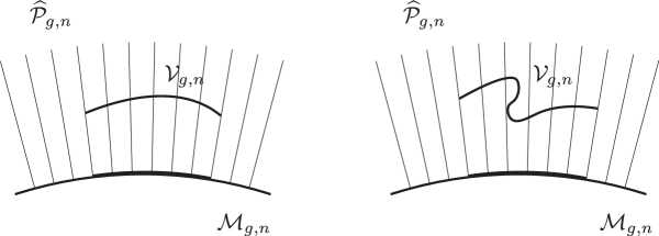
Figure 1: Left: A string vertex ${\cal V}_{g,n}$ that is a piece of a section over ${\cal M}_{g,n}$. Right: A string vertex ${\cal V}_{g,n}$ that is not a piece of a section over ${\cal M}_{g,n}$. In both cases the projection $\pi$ maps ${\cal V}_{g,n}$ to its image with degree one.

When the string vertices are used together with a propagator to form Feynman graphs of string field theory, the result is some submanifold ${\cal F}_{g,n}$ in $\widehat{\cal P}_{g,n}$. It is traditionally required that ${\cal F}_{g,n}$ should be a full section of the bundle $\widehat{\cal P}_{g,n}$, so that the map ${\cal F}_{g,n}\to{\cal M}_{g,n}$ is a homeomorphism. Again, this is not necessary: all that is required is that the map ${\cal F}_{g,n}\to{\cal M}_{g,n}$ is of degree one. Such a map is surjective.

This is enough to imply that the integral over ${\cal F}_{g,n}$ of any differential form pulled back from ${\cal M}_{g,n}$ will be the same as the integral over ${\cal M}_{g,n}$. Since the integrand for on-shell string states is a top-form on ${\cal M}_{g,n}$, this implies that the amplitude for on-shell string states computed by integrating over ${\cal M}_{g,n}$ coincides with that computed using string field theory Feynman rules.

It is sometimes useful to consider string vertices which are not sub-manifolds of $\widehat{\cal P}_{g,n}$, but rather singular chains of degree $6g-6+2n$. This is reasonable, because the purpose of introducing string vertices is to integrate over them, and there is a well-behaved theory of integration pairing differential forms with singular chains. In this generality, the string vertices ${\cal V}_{g,n}$ must satisfy two constraints:

1. The chain ${\cal V}$ must satisfy the geometric master equation (1.1).

2. The chain ${\cal F}_{g,n}$, constructed as Feynman diagrams using ${\cal V}$ and a propagator, must, when pushed forward to ${\cal M}_{g,n}$, represent the fundamental homology class of ${\cal M}_{g,n}$.

In the case that ${\cal F}_{g,n}$ is represented by a submanifold of $\widehat{\cal P}_{g,n}$, this second constraint implies that the map ${\cal F}_{g,n}\to{\cal M}_{g,n}$ is of degree one. Without the assumption that ${\cal F}_{g,n}$ is a submanifold, this constraint implies that the integral over ${\cal F}_{g,n}$ of a differential form on $\widehat{\cal P}_{g,n}$ which is pulled back from ${\cal M}_{g,n}$ coincides with the integral over ${\cal M}_{g,n}$.

For string vertices in this sense, existence and uniqueness (up to canonical transformations) was proved in [7]. We give a largely self-contained review and detailed elaboration of these arguments in section 2. The earlier discussion of these matters in the physics literature [8, 4] did not address a priori existence, and uniqueness was shown assuming the vertices are submanifolds and partial sections of $\widehat{\cal P}_{g,n}$. We also show that the second condition listed above holds for any string vertices that satisfy the first condition. Thus satisfying the master equation is all that is required of ${\cal V}$.

One approach to determine the string vertices explicitly is through a (conformal) minimal area problem [9]. On each Riemann surface in ${\cal M}_{g,n}$, the problem asks for the metric of least area for a fixed systole (the length of the shortest closed geodesic). The minimal area metrics for genus zero and $n\geq 3$ are well known and arise from Jenkins-Strebel quadratic differentials. For genus one or greater, the minimal area metrics are partially known. As of now there is no general proof of existence of the minimal area metrics, presumably because it is not known how singular the metrics can be. Recently, however, Headrick and one of us used convex optimization to develop theoretical and computational tools to deal with these minimal area metrics, to find accurate numerical solutions for previously unknown metrics [10, 11] and, with Naseer, to obtain insight into the closely related Riemannian isosytolic problem [12]. The new metrics do not seem to be particularly singular, and one could expect that an existence proof will be developed in the near future. Using the minimal area metrics there is a simple prescription to define string vertices that satisfy the geometric master equation. Since minimal area metrics are unique, the vertices are pieces of sections over ${\cal M}_{g,n}$ and the Feynman rules generate full sections over ${\cal M}_{g,n}$.

A new and intriguing approach to the question of finding string vertices was recently developed by Moosavian and Pius [13, 14] using the framework of hyperbolic geometry. The use of hyperbolic geometry is particularly attractive due to recent progress using Teichmüller spaces of hyperbolic metrics in order to compute integrals over the moduli spaces of Riemann surfaces [15, 16, 17] (for a review of some of these ideas see [18]). The authors considered hyperbolic metrics (metrics of Gaussian curvature $K=-1$) on punctured Riemann surfaces in ${\cal M}_{g,n}$ and defined subsets that to first approximation are string vertices. The metrics have cusps at the punctures and can be used to define local coordinates around them. The boundaries of the coordinate disks, however, are horocycles rather than geodesics. This implies that the sewing of these surfaces do not yield exactly hyperbolic metrics. The vertices and local coordinates around the punctures must then be corrected, and the authors discuss how to do this to first order in a cutoff parameter using results by Wolpert [19] and Obitsu and Wolpert [20].

Motivated by their work and following a suggestion of one of us [21], we give here a simple and explicit hyperbolic construction of string vertices. Instead of starting with ${\cal M}_{g,n}$, however, we use moduli spaces of hyperbolic metrics on surfaces of genus $g$ and $n$ geodesic boundaries. By restricting the metrics to those for which the boundaries all have length $L$ we consider the moduli space ${\cal M}_{g,n,L}$. On these surfaces the systole is defined as the shortest geodesic that is not a boundary component. We define string vertices as systolic subsets of these moduli spaces: they include all surfaces with systole greater than or equal to $L$. Namely, surfaces belonging to a vertex have no geodesics of length less than $L$. For each surface in the vertices we turn the $n$ boundaries into $n$ punctured disks by grafting flat semi-infinite cylinders of circumference $L$. This is a canonical operation giving us a homeomorphism from ${\cal M}_{g,n,L}$ to ${\cal M}_{g,n}$. It is not hard to show that for any $L<L_{*}=2\,\hbox{arcsinh}\,1$ the string vertices satisfy exactly the geometric master equation. As a result the vertices define a closed string field theory that satisfies the BV master equation exactly. A key role in the construction is played by the collar theorems of hyperbolic geometry [22]: the collars about the geodesic boundaries play the same role as stubs do in minimal area metrics: they prevent the creation closed curves shorter than $L$ upon sewing. Vertices with different values of $L$ are equivalent up to BV canonical transformations.

We use the work of Mondello [23] to explain that the hyperbolic string vertices are in fact pieces of sections in $\widehat{\cal P}_{g,n}$. To form the Feynman diagrams of this theory, one joins the boundaries on surfaces belonging to string vertices by attaching annuli, representing the propagator. The string field theory does not prescribe a metric on the annuli, but it is clear that making the annulus into a flat cylinder of circumference $L$ defines a continuous metric throughout the surface. Note that a hyperbolic metric on the annulus would give a metric that is discontinuous at the seams and is therefore not hyperbolic on the whole surface. The mixed metric, hyperbolic on the vertices and flat on the cylinders, is natural. It arises in the theory of $\mathbb{CP}^{1}$ projective structures on surfaces, and in the definition of grafting across measured geodesic laminations. In such theory the above metric, called the Thurston metric, arises naturally as the Kobayashi metric in the category of $\mathbb{CP}^{1}$ surfaces. Results by Dumas and Wolf [25] hint that we may be also getting sections from the Feynman region.

Note added: We were informed by Jørgen E. Andersen that he also showed that the systolic sets suggested in [21] solve the quantum master equation [26].

2 Existence and uniqueness of string vertices

In this section we will review the homological argument of [7] that proves the existence of the string vertices, and their uniqueness up to canonical transformation. (The super-string version of this argument has recently been provided by Moosavian and Zhou [24]). We also show how the construction guarantees that the chain constructed as Feynman diagrams represents the fundamental homology class of ${\cal M}_{g,n}$.

The material in this section provides perspective on the problem of finding explicit string vertices, but is not required for the construction of hyperbolic vertices in the subsequent sections.

2.1 Canonical transformations

Suppose that we have some collection ${\cal V}_{g,n}$ of string vertices. For this section, we do not require that the ${\cal V}_{g,n}$ are represented by submanifolds of $\widehat{\cal P}_{g,n}$. All we ask is that the ${\cal V}_{g,n}$ are singular chains with real coefficients, that is elements of $C_{6g-6+2n}(\widehat{\cal P}_{g,n})$.

If we have some collection ${\cal W}_{g,n}\in C_{6g-6+2n+1}(\widehat{\cal P}_{g,n})$, then we can vary the string vertices ${\cal V}_{g,n}$ by

$$\delta_{{\cal W}}{\cal V}=\{{\cal V}\,,{\cal W}\}+\hbar\Delta{\cal W}+\partial{\cal W}\,,$$ (2.1)

where, as before, ${\cal V}=\sum\hbar^{g}{\cal V}_{g,n}$, ${\cal W}=\sum\hbar^{g}{\cal W}_{g,n}$. It is automatic that this variation of ${\cal V}$ still satisfies the quantum master equation, to leading order in $\delta_{{\cal W}}{\cal V}$:

$$\begin{split}&\tfrac{1}{2}\{{\cal V}+\delta_{{\cal W}}{\cal V},{\cal V}+\delta_{{\cal W}}{\cal V}\}+\hbar\Delta({\cal V}+\delta_{{\cal W}}{\cal V})+\partial(V+\delta_{{\cal W}}{\cal V})\\ &=\bigl{\{}\partial{\cal V}+\hbar\,\Delta{\cal V}+\tfrac{1}{2}\{{\cal V}\,,{\cal V}\}\,,{\cal W}\bigr{\}}+O((\delta_{{\cal W}}{\cal V})^{2})=0\,.\end{split}$$ (2.2)

A variation of this form is an infinitesimal canonical transformation.

Two sets of string vertices which are related by canonical transformations like this yield equivalent string field theories. To understand this, let us recall some background on how the string field theory action is constructed.

The string action $S_{\cal V}$ associated to a set of vertices is given by

$$S_{\cal V}(\psi)=S_{0,2}+I_{\cal V}(\psi)\,,$$ (2.3)

where $S_{0,2}={1\over 2}\langle\psi,Q\psi\rangle$ is the kinetic term and does not depend on the vertices. Moreover, $I_{\cal V}(\psi)$ denotes the interactions, obtained by integrating the correlators of the closed string field $\psi$ over the moduli spaces in ${\cal V}$. The compatibility of the BV anti-bracket in string field theory with that defined by cutting and gluing Riemann surfaces tells us that for chains $A,B$ we have [5]:

$$I_{\Delta A}=-\Delta I_{A}\,,\quad I_{\{A,B\}}=-\{I_{A},I_{B}\}\,,\quad I_{\partial A}=-\{S_{0,2},I_{A}\}\,.$$ (2.4)

It now follows from (2.3) and the expression for $\delta_{\cal W}{\cal V}$ that

$$\begin{split}S_{{\cal V}+\delta_{\cal W}{\cal V}}=&\ S_{\cal V}+I_{\delta_{\cal W}{\cal V}}\\ =&\ S_{\cal V}+I_{\{{\cal V}\,,{\cal W}\}+\hbar\Delta{\cal W}+\partial{\cal W}}\\ =&\ S_{\cal V}-\{I_{\cal V}\,,I_{\cal W}\}-\hbar\Delta I_{\cal W}-\{S_{0,2},{\cal W}\}\\ =&\ S_{\cal V}-\{S_{\cal V}\,,I_{\cal W}\}-\hbar\Delta I_{\cal W}\,,\end{split}$$ (2.5)

showing that the action for the new vertices is obtained by an infinitesimal canonical transformation of the original action. Indeed, the transformation $\delta S=\hbar\Delta\epsilon+\{S,\epsilon\}$ with $\epsilon$ an odd parameter leaves the master equation $\hbar\Delta S+{1\over 2}\{S,S\}=0$ unchanged. This shows that vertices related by a canonical transformation can be regarded as equivalent. Observables transform under canonical transformations and their expectation values are also unchanged.

2.2 Existence of string vertices

The argument for existence of string vertices is inductive. We start by fixing ${\cal V}_{0,3}$, which is of dimension $0$, to be $\mathbb{CP}^{1}$ with marked points $0,1,\infty$ and some choice of coordinates around the marked points, invariant under the action of $S_{3}$ permuting the marked points.

For the inductive step, fix a pair of integers $(g,n)$. We assume, by induction, that we have constructed ${\cal V}_{g^{\prime},n^{\prime}}$ for all $(g^{\prime},n^{\prime})$ with $g^{\prime}<g$, or with $g^{\prime}=g$ and $n^{\prime}<n$. We assume that the ${\cal V}_{g^{\prime},n^{\prime}}$ we have constructed satisfy the master equation. We also assume that ${\cal V}_{g^{\prime},n^{\prime}}$ is invariant under the action of $S_{n^{\prime}}$ permuting the marked points.

We need to find ${\cal V}_{g,n}$ satisfying

$$\partial{\cal V}_{g,n}=-\Delta{\cal V}_{g-1,n+2}\ -\ \tfrac{1}{2}\hskip-10.0pt\sum_{\begin{subarray}{c}g_{1}+g_{2}=g\\ n_{1}+n_{2}=n+2\end{subarray}}\hskip-5.0pt\{{\cal V}_{g_{1},n_{1}},{\cal V}_{g_{2},n_{2}}\}\ \equiv{\cal O}_{g,n}\,.$$ (2.6)

The right hand side ${\cal O}_{g,n}$ of this equation is a $(6g-6+2n)-1$ chain on $\widehat{\cal P}_{g,n}$. It is build entirely from ${\cal V}_{g^{\prime},n^{\prime}}$ which we have already constructed in our induction. By construction, ${\cal O}_{g,n}$ is an $S_{n}$ invariant chain, as required for ${\cal V}_{g,n}$ to be $S_{n}$ invariant as well.

Our inductive assumption that the ${\cal V}_{g^{\prime},n^{\prime}}$ satisfy the quantum master equation implies that

$$\partial{\cal O}_{g,n}=0\,.$$ (2.7)

This can be checked by writing $\partial{\cal V}=-\hbar\Delta{\cal V}-{1\over 2}\{{\cal V},{\cal V}\}$ and confirming that $\partial$ kills the right-hand side using $\{\{{\cal V},{\cal V}\},{\cal V}\}=0$. The problem of constructing the string vertex ${\cal V}_{g,n}$ satisfying (2.6) amounts to showing that the homology class

$$[{\cal O}_{g,n}]\in H_{6g-6+2n-1}(\widehat{\cal P}_{g,n})^{S_{n}}$$ (2.8)

vanishes. The superscript $S_{n}$ indicates that we are focusing on the homology of $S_{n}$-invariant chains.

To prove that $[{\cal O}_{g,n}]=0$, we will show that the homology group $H_{6g-6+2n+1}(\widehat{\cal P}_{g,n})^{S_{n}}$ is zero. The proof of this consists of two steps.

1. First, we show that $\widehat{\cal P}_{g,n}$ is homotopy equivalent to ${\cal M}_{g,n}$. This implies that the homology groups of $\widehat{\cal P}_{g,n}$ and of ${\cal M}_{g,n}$ are isomorphic.

2. Then, we show that $H_{6g-6+2n-1}({\cal M}_{g,n})^{S_{n}}$ is zero.

2.2.1 Proving the homotopy equivalence $\widehat{\cal P}_{g,n}\simeq{\cal M}_{g,n}$

Let us recall that $\widehat{\cal P}_{g,n}$ is the moduli space of Riemann surfaces $\Sigma$ with $n$ embedded discs $D_{1},\dots,D_{n}$. We assume here that the closures of the $D_{i}$ are disjoint. On each disc, we have a coordinate function $z_{i}$, defined up to rotation, such that $D_{i}=\{|z_{i}|\leq 1\}$, and we assume that $z_{i}$ extends analytically to a small neighbourhood in $\Sigma$ of the closure $\overline{D}_{i}$ of the disc.

This moduli space can be described equivalently as follows. Consider the moduli space $\widehat{\cal P}^{\prime}_{g,n}$ of Riemann surfaces with $n$ boundary components $b_{i}$, and a coordinate $\theta_{i}$ on each boundary component, defined up to a shift. We assume that the coordinate $\theta_{i}$ has the following properties:

1. $\theta_{i}$ has range $2\pi$.

2. $\theta_{i}$ is real analytic.

3. The vector field $\partial_{\theta_{i}}$ points in the direction given by the orientation of the boundary component $b_{i}$ which is induced from the orientation of the bulk surface.

Suppose, near some point in one of the boundary components, we choose coordinates $z=x+\mathsf{i}y$ where the boundary is at $y=0$ and a local patch of the surface is in the upper half-plane $y\geq 0$. Then, $\theta_{i}$ is some function $F_{i}(x)$. Our assumption that $\theta_{i}$ is real-analytic means $F_{i}$ is a real-analytic function of $x$, and so represented by a convergent power series. Because of this, $F_{i}(z)$ will also converge in some domain. This implies that $\theta_{i}$ is the boundary value of the holomorphic function $F_{i}(z)$, and because $\theta_{i}$ provides a coordinate on the boundary, $F_{i}(z)$ must provide a holomorphic coordinate in some neighbourhood of the boundary. This fact will be key for gluing surfaces.

There is an isomorphism $\widehat{\cal P}_{g,n}\cong\widehat{\cal P}^{\prime}_{g,n}$, as we now explain. For a marked surface $\Sigma$ in $\widehat{\cal P}_{g,n}$, we obtain a surface $\Sigma^{\prime}$ with $n$ boundary components $b_{i}$ by removing the discs $D_{i}$. We define a coordinate $\theta_{i}$ on each $b_{i}$ by setting

$$\theta_{i}=\operatorname{Im}\log z_{i}.$$ (2.9)

Since $z_{i}$ is defined up to a phase, $\theta_{i}$ is defined up to a shift. Further, the functions $\theta_{i}$ are all analytic and of range $2\pi$ as desired.

Conversely, given a surface $\Sigma^{\prime}\in\widehat{\cal P}^{\prime}_{g,n}$, we obtain a surface in $\widehat{\cal P}_{g,n}$ by gluing a disc $\overline{D}_{i}=\{\left|z_{i}\right|\leq 1\}$ to the boundary component $b_{i}$ of $\Sigma$. This gluing identifies $\operatorname{Im}\log z_{i}$ with $\theta_{i}$. Because $\operatorname{Im}\log z_{i}$ and $\theta_{i}$ are, locally, the boundary values of holomorphic coordinates in a region of $\overline{D}_{i}$ and of $\Sigma^{\prime}$, respectively, the glued surface is naturally holomorphic.

There is a map from $\widehat{\cal P}^{\prime}_{g,n}$ to the moduli space ${\cal M}^{\prime}_{g,n}$ of Riemann surfaces with boundary, given by forgetting the coordinates $\theta_{i}$. We will show that this map is homotopy equivalence. To show this, it suffices to show that the fibres are contractible (because $\widehat{\cal P}^{\prime}_{g,n}$ is a fibration over ${\cal M}^{\prime}_{g,n}$). This means that we need to show that the space of possible choices of coordinate $\theta_{i}$ on each boundary component $b_{i}$ of ${\cal M}^{\prime}_{g,n}$ is contractible.

Let us fix reference coordinates $\theta_{i}$ on each boundary component $b_{i}$, and write any other coordinate system as $\widetilde{\theta}_{i}=F_{i}(\theta_{i})$. Because each coordinate is defined up to a shift, we can assume that $F_{i}(0)=0$. For this new coordinate to have range $2\pi$ we must have $F_{i}(\theta_{i}+2\pi)=F_{i}(\theta_{i})+2\pi$. The compatibility with the orientation, and the fact that $F_{i}(\theta_{i})$ must define a new coordinate system, tells us that $\partial_{\theta_{i}}F_{i}(\theta_{i})>0$.

We need to show that the space of possible choices of functions $F_{i}(\theta_{i})$ satisfying these constraints is contractible. The contracting homotopy is simply given by the one-parameter family

$$F_{i}^{\lambda}(\theta_{i})=\lambda\theta_{i}+(1-\lambda)F_{i}(\theta_{i})\,,$$ (2.10)

for $0\leq\lambda\leq 1$. This satisfies the same properties as $F_{i}(\theta_{i})$, that is $\partial_{\theta_{i}}F_{i}^{\lambda}(\theta_{i})>0$, $F_{i}^{\lambda}(0)=0$, and $F_{i}^{\lambda}(\theta_{i}+2\pi)=F_{i}^{\lambda}(\theta_{i})+2\pi$. Therefore $F_{i}^{\lambda}(\theta_{i})$ defines a one-parameter family of real analytic coordinates connecting that given by $\theta_{i}$ to that given by $F_{i}(\theta_{i})$.

We have shown that $\widehat{\cal P}_{g,n}$ is isomorphic to $\widehat{\cal P}^{\prime}_{g,n}$, which is homotopy equivalent to the moduli space of Riemann surfaces with boundary. The latter is known to be homeomorphic to ${\cal M}_{g,n}\times(\mathbb{R}_{>0})^{n}$, and so is homotopy equivalent to ${\cal M}_{g,n}$.

2.2.2 Homology vanishing for ${\cal M}_{g,n}$

The homotopy equivalence between $\widehat{\cal P}_{g,n}$ and ${\cal M}_{g,n}$ shows that they have isomorphic homology groups. Next, we will show that $H_{6g-6+2n-1}({\cal M}_{g,n})$ vanishes except when $(g,n)=(0,4)$.

By Poincaré duality, we can identify $H_{6g-6+2n-1}({\cal M}_{g,n})$ with $H^{1}(\overline{{\cal M}}_{g,n},\overline{{\cal M}}_{g,n}\setminus{\cal M}_{g,n})$ (here we consider relative cohomology of the Deligne-Mumford space, relative to the complement of the locus of smooth Riemann surfaces). So it suffices to show that this $H^{1}$ cohomology group vanishes. To do this, we first consider the exact sequence of relative cohomology groups

$$0\to H^{0}(\overline{{\cal M}}_{g,n})\to H^{0}(\partial\overline{{\cal M}}_{g,n})\to H^{1}(\overline{{\cal M}}_{g,n},\partial\overline{{\cal M}}_{g,n})\to H^{1}(\overline{{\cal M}}_{g,n})\to\dots$$ (2.11)

It is known that $H^{1}(\overline{{\cal M}}_{g,n})=0$, and that $\partial\overline{{\cal M}}_{g,n}$ is connected except for $(g,n)=(0,4)$. This implies that, as desired,

$$H^{1}(\overline{{\cal M}}_{g,n},\partial\overline{{\cal M}}_{g,n})=0\,,\quad\hbox{for}\ \ (g,n)\neq(0,4)\,.$$ (2.12)

For $(g,n)=(0,4)$, the group $H_{1}({\cal M}_{0,4})$ does not vanish but the $S_{4}$ invariant group $H_{1}({\cal M}_{0,4})^{S_{4}}$ does. The moduli space ${\cal M}_{0,4}$ is a $\mathbb{CP}^{1}$ with three points removed, as we can set the first three marked points to $0,1,\infty$ and the last marked point $z_{4}$ can be anywhere else on $\mathbb{CP}^{1}$.

The first homology group of ${\cal M}_{0,4}$ is two-dimensional, parametrized by the cycles where the last marked point $z_{4}$ moves around $0$ or moves around $1$. This is some two-dimensional representation of $S_{4}$, and we need to show it has no trivial subrepresentations. To do this, it suffices to show that it has no trivial subrepresentations as a representation of the copy of $S_{3}$ in $S_{4}$ which permutes the first three marked point. As a representation of $S_{3}$, it is clear that this is the standard irreducible two-dimensional representation, which is the complement of the trivial representation in the three dimensional permutation representation. Therefore, there are no trivial subrepresentations. This completes the inductive proof of existence of the string vertices.

2.3 Uniqueness of string vertices

Uniqueness, up to BV canonical transformations, is proved by a similar inductive argument. To understand this, we need to discuss the exponentiated form of the canonical transformation.

Let ${\cal V}$ be a set of string vertices, and ${\cal W}$ a collection ${\cal W}_{g,n}\in\Gamma_{6g-6+2n+1}(\widehat{\cal P}_{g,n})$ of $S_{n}$-invariant singular chains which define an infinitesimal canonical transformation. We define a family ${\cal V}(t)$ of string vertices such that ${\cal V}(0)={\cal V}$ and asking that they satisfy the differential equation

$$\frac{\mathrm{d}}{\mathrm{d}t}{\cal V}(t)=\delta_{\cal W}{\cal V}(t)\,.$$ (2.13)

where

$$\delta_{\cal W}{\cal V}=\{{\cal V}\,,{\cal W}\}+{\cal B}_{\cal W}\,,\qquad{\cal B}_{\cal W}\equiv\partial{\cal W}+\hbar\Delta{\cal W}\,,$$ (2.14)

is the infinitesimal canonical transformation defined before, and we have introduced the symbol ${\cal B}_{\cal W}$ to denote the part of the transformation that is not linear on ${\cal V}$.

If ${\cal V}$ satisfies the master equation, then so does ${\cal V}(t)$ for all $t$. To see this, let us write the master equation for ${\cal V}(t)$ in the form the form $M_{\cal V}(t)=0$ by defining

$$M_{\cal V}(t)\equiv\partial{\cal V}(t)+\hbar\Delta{\cal V}(t)+\tfrac{1}{2}\left\{{\cal V}(t),{\cal V}(t)\right\}\,.$$ (2.15)

Clearly $M_{\cal V}(0)=0$ since the string vertices ${\cal V}$ satisfy the master equation. A short calculation using the differential equation (2.13) shows that $M_{\cal V}$ satisfies the equation

$$\frac{\mathrm{d}M_{{\cal V}}}{\mathrm{d}t}=\{M_{{\cal V}}(t)\,,{\cal W}\}\,.$$ (2.16)

This equation implies that if $M_{\cal V}(0)=0$ all derivatives of $M_{\cal V}(t)$ will vanish at $t=0$. This shows $M_{\cal V}(t)$ vanishes at all times.

We can write the solution of (2.13) for the instantaneous vertices by taking multiple derivatives, evaluating at $t=0$ and writing the Taylor series. This gives

$${\cal V}(t)={\cal V}+t\delta_{\cal W}{\cal V}+\tfrac{1}{2}t^{2}\{\delta_{\cal W}{\cal V},{\cal W}\}+\tfrac{1}{3!}t^{3}\bigl{\{}\{\delta_{\cal W}{\cal V},{\cal W}\},{\cal W}\bigr{\}}+\cdots\ .$$ (2.17)

We define the exponential of the canonical transformation via $\exp\left(t\delta_{{\cal W}}\right){\cal V}\equiv{\cal V}(t)$. Note that the series solution does not fit the naive expansion of the exponential in that we do not encounter nor define iterated variations $\delta_{{\cal W}}\delta_{{\cal W}}{\cal V}$. The definition implies that

$$\exp\left(\delta_{{\cal W}}\right){\cal V}\equiv{\cal V}+\delta_{\cal W}{\cal V}+\tfrac{1}{2}\{\delta_{\cal W}{\cal V},{\cal W}\}+\tfrac{1}{3!}\bigl{\{}\{\delta_{\cal W}{\cal V},{\cal W}\},{\cal W}\bigr{\}}+\cdots\ .$$ (2.18)

With $\delta_{\cal W}{\cal V}=\{{\cal V},{\cal W}\}+{\cal B}_{\cal W}$ we have

$$\begin{split}\exp\left(\delta_{{\cal W}}\right){\cal V}=&\ \ {\cal V}+\{{\cal V},{\cal W}\}+\tfrac{1}{2}\{\{{\cal V},{\cal W}\},{\cal W}\}+\tfrac{1}{3!}\bigl{\{}\{\{{\cal V},{\cal W}\},{\cal W}\},{\cal W}\bigr{\}}+\cdots\\ &+{\cal B}_{\cal W}+\tfrac{1}{2}\{{\cal B}_{\cal W},{\cal W}\}+\tfrac{1}{3!}\bigl{\{}\{{\cal B}_{\cal W},{\cal W}\},{\cal W}\bigr{\}}+\cdots\ .\end{split}$$ (2.19)

This equation will be useful below.

Now let us turn to the uniqueness of the string vertices. Suppose that ${\cal V}_{g,n}$, ${\cal V}^{\prime}_{g,n}$ are two sets of string vertices, both satisfying the master equation. Our goal is to show inductively that there exists a sequence of $S_{n}$-invariant singular chains ${\cal W}_{g,n}\in C_{6g-6+2n+1}(\widehat{\cal P}_{g,n})$ such that

$$\exp\left(\delta_{{\cal W}}\right){\cal V}={\cal V}^{\prime}.$$ (2.20)

To perform the induction it is useful to introduce a partial ordering on the collection of pairs $(g,n)$ of non-negative integers with $2g-2+n>0$. We say $(g^{\prime},n^{\prime})<(g,n)$ if $g^{\prime}<g$, or if $g^{\prime}=g$ and $n^{\prime}<n$.

The initial step of the induction is $(g,n)=(0,3)$, in which case ${\cal V}_{0,3}$ and ${\cal V}^{\prime}_{0,3}$ are both $S_{3}$ invariant points in $\widehat{\cal P}_{0,3}$. Since this space is connected, we let ${\cal W}_{0,3}$ be a $S_{3}$-invariant path connecting ${\cal V}_{0,3}$ to ${\cal V}^{\prime}_{0,3}$. Viewing ${\cal W}_{0,3}$ as a one-chain, we have

$$\partial{\cal W}_{0,3}={\cal V}^{\prime}_{0,3}-{\cal V}_{0,3}\,.$$ (2.21)

This implies that we have satisfied (2.20) to leading order

$$\left(\exp\left(\delta_{{\cal W}_{0,3}}\right){\cal V}\right)_{0,3}={\cal V}^{\prime}_{0,3}\,,$$ (2.22)

where for any chain $X$ we let $(X)_{g,n}$ denote the piece that belongs to $\widehat{\cal P}_{g,n}$. Equation (2.22) can be checked using (2.19) to evaluate the left-hand side. This means that the string vertices on the left and right of (2.20) agree for $(g,n)=(0,3)$.

Next, we assume that we have constructed ${\cal W}_{g^{\prime},n^{\prime}}$ by induction for all $(g^{\prime},n^{\prime})<(g,n)$. We let ${\cal W}_{<(g,n)}$ be the totality of the ${\cal W}_{g^{\prime},n^{\prime}}$ that we have already constructed. By induction, we will assume that

$$\left(\exp\left(\delta_{{\cal W}_{<(g,n)}}\right){\cal V}\right)_{g^{\prime},n^{\prime}}=\,\hbar^{g^{\prime}}{\cal V}^{\prime}_{g^{\prime},n^{\prime}}\,,$$ (2.23)

for all $(g^{\prime},n^{\prime})<(g,n)$.

To continue the induction, we need to find some ${\cal W}_{g,n}$ such that

$$\left(\exp\left(\delta_{{\cal W}_{<(g,n)}}+\hbar^{g}\delta_{{\cal W}_{g,n}}\right){\cal V}\right)_{g^{\prime},n^{\prime}}=\,\hbar^{g^{\prime}}\,{\cal V}^{\prime}_{g^{\prime},n^{\prime}}\,,$$ (2.24)

for all $(g^{\prime},n^{\prime})\leq(g,n)$. Changing the canonical transformation by adding $\hbar^{g}{\cal W}_{g,n}$ does not affect the left hand side of this equation for $(g^{\prime},n^{\prime})<(g,n)$. It only changes it for $(g^{\prime},n^{\prime})=(g,n)$. A bit of analysis shows that

$$\left(\exp\left(\delta_{{\cal W}_{<(g,n)}}+\hbar^{g}\delta_{{\cal W}_{g,n}}\right){\cal V}\right)_{g,n}=\,\hbar^{g}\,\partial{\cal W}_{g,n}+\left(\exp\left(\delta_{{\cal W}_{<(g,n)}}\right){\cal V}\right)_{g,n}\,.$$ (2.25)

Indeed, with ${\cal W}={\cal W}_{<(g,n)}+\hbar^{g}{\cal W}_{g,n}$, one can check using (2.19) that the contributions to a $(g,n)$ chain from ${\cal W}_{g,n}$ arise only from ${\cal B}_{\cal W}$, and then only from the term with $\partial$. In checking this it helps to note that for any $X_{g,n}$ and any $Y$, we have $(\{X_{g,n},Y\})_{\leq(g,n)}=0$, namely, the left hand side only contains chains higher up in the ordering. Similarly, for higher nested objects $(\bigl{\{}\{X_{g,n},Y\},Z\bigr{\}})_{\leq(g,n)}=0$.

It is useful to define

$${\cal V}^{\prime\prime}:=\exp\left(\delta_{{\cal W}_{<(g,n)}}\right){\cal V}\,.$$ (2.26)

With this, the induction assumption above states that ${\cal V}^{\prime\prime}_{g^{\prime},n^{\prime}}={\cal V}^{\prime}_{g^{\prime},n^{\prime}}$ for all $(g^{\prime},n^{\prime})<(g,n)$. To continue the induction and on account of (2.25), the chain ${\cal W}_{g,n}$ is required to satisfy

$$\partial{\cal W}_{g,n}={\cal V}^{\prime}_{g,n}-{\cal V}^{\prime\prime}_{g,n}\,.$$ (2.27)

The right hand side is a singular chain in $C_{6g-6+2n}(\widehat{\cal P}_{g,n})$. This equation can only have a solution if the right hand side is in the kernel of the boundary operator $\partial$. To see this, we note that the master equation expresses $\partial{\cal V}^{\prime}_{g,n}$ and $\partial{\cal V}^{\prime\prime}_{g,n}$ in terms of ${\cal V}^{\prime}_{g^{\prime},n^{\prime}}$ and ${\cal V}^{\prime\prime}_{g^{\prime},n^{\prime}}$, respectively, for $(g^{\prime},n^{\prime})<(g,n)$. These spaces are the same by the induction assumption, so that, as expected,

$$\partial\,({\cal V}^{\prime\prime}_{g,n}-{\cal V}^{\prime}_{g,n})=0.$$ (2.28)

To show that there exists a solution ${\cal W}_{g,n}$ to (2.27), it suffices to show that the homology group $H_{6g-6+2n}(\widehat{\cal P}_{g,n})$ is zero (this, of course implies it also vanishes for $S_{n}$-invariant chains). This is the case as long as $(g,n)\neq(0,3)$. The point is that $\widehat{\cal P}_{g,n}$ is homotopy equivalent to ${\cal M}_{g,n}$, and ${\cal M}_{g,n}$ is a non-compact orbifold of dimension $6g-6+2n$. By Poincaré duality, $H_{6g-6+2n}({\cal M}_{g,n})$ is isomorphic to $H^{0}(\overline{{\cal M}}_{g,n},\overline{{\cal M}}_{g,n}\setminus{\cal M}_{g,n})$, the cohomology of the Deligne-Mumford compactification relative to the complement of the open subset of smooth surfaces. This cohomology group vanishes, except in the case $(g,n)=(0,3)$. This completes the proof of uniqueness (up to canonical transformations) of the string vertices.

2.4 Representing the fundamental homology class of moduli space

We have not, however, addressed an important part of the story. Given a collection ${\cal V}_{g,n}$ of string vertices, we let ${\cal F}_{g,n}$ be the corresponding chains built using Feynman diagrams with ${\cal V}$ as the vertices. We need to show that when we push forward the chain ${\cal F}_{g,n}$ to ${\cal M}_{g,n}$, we find a representative of the fundamental homology class of ${\cal M}_{g,n}$.

To understand this, we need a few more details on the construction of ${\cal F}_{g,n}$. We take as our propagator the flat cylinder of fixed radius and arbitrary length $\tau$. According to the usual string field theory Feynman rules, when we glue in the cylinder, we allow a “twist”. This means that adding a propagator increases the dimension of a chain by two: one for the length $\tau$ and one for the twist parameter.

Let us include into our propagator the infinite cylinder $\tau=\infty$. Conformally, having a cylinder of infinite length is equivalent to having a cylinder of finite length but with a circle of radius zero in the middle. We will interpret the infinite length cylinder in this way, as two very long “cigars” meeting at their tips. In terms of algebraic geometry, we can view it as the nodal curve $zw=0$. At infinite length, the twist parameter in the Feynman diagrams is irrelevant, as we can rotate each cigar independently. This should be familiar: when we glue two Riemann surfaces along a common boundary to produce a smooth surface, we need to specify the twist to perform the gluing. But when we glue two surfaces with marked points to produce a surface with a nodal singularity, no such choice is necessary.

If we include this infinite cylinder in our propagator, then we see that ${\cal F}_{g,n}$ is a chain in the space $\widehat{\overline{{\cal P}}}_{g,n}$: this is the space consisting of possibly nodal surfaces in the Deligne-Mumford compactification $\overline{{\cal M}}_{g,n}$ equipped with coordinates around the punctures, defined up to rotation.

By forgetting the coordinates around the punctures, there is a map

$$\pi:\widehat{\overline{{\cal P}}}_{g,n}\to\overline{{\cal M}}_{g,n}.$$ (2.29)

There is a corresponding map $\pi_{\ast}$ on singular chains, and our goal is to show that $\pi_{\ast}{\cal F}_{g,n}$ is a representative for the fundamental homology class of $\overline{{\cal M}}_{g,n}$.

To show this, we will first show that the chain ${\cal F}_{g,n}$ is closed. The boundary $\partial{\cal F}_{g,n}=0$ has three contributions:

1. Contributions from the boundary of the vertices ${\cal V}_{g^{\prime},n^{\prime}}$ making up ${\cal F}_{g,n}$.

2. Contributions from surfaces where the length $\tau$ of a propagator is zero.

3. Contributions from surfaces where the length $\tau$ of the propagator is $\infty$.

The first two types of contributions cancel each other exactly, because of the master equation satisfied by the vertices ${\cal V}$. The key point is that the propagator at $\tau=0$ performs precisely the “twist-gluing” defining the operators $\Delta$ and $\{\cdot\,,\,\cdot\}$ in the master equation. The third contribution, that from $\tau=\infty$, vanishes as well. This is because the twist parameter in the gluing is not present at $\tau=\infty$, so that this locus is not a boundary, but rather of codimension $2$. This completes the proof that ${\cal F}_{g,n}$ is closed.

Since ${\cal F}_{g,n}$ is a cycle (i.e. closed chain) in $C_{6g-6+2n}(\widehat{\overline{{\cal P}}}_{g,n})$, its pushforward $\pi_{\ast}{\cal F}_{g,n}$ to $\overline{{\cal M}}_{g,n}$ is a cycle in $C_{6g-6+2n}({\overline{{\cal M}}}_{g,n})$. Because $\overline{{\cal M}}_{g,n}$ is a compact orbifold, Poincaré duality tells us that $H_{6g-6+2n}(\overline{{\cal M}}_{g,n})=\mathbb{R}$. It follows that there is some constant $c_{g,n}\in\mathbb{R}$ such that

$$[\pi_{\ast}{\cal F}_{g,n}]=c_{g,n}[\overline{{\cal M}}_{g,n}].$$ (2.30)

We need to show that $c_{g,n}=1$.

If the cycle ${\cal F}_{g,n}$ was itself a manifold or an orbifold, then the statement that $[\pi_{\ast}{\cal F}_{g,n}]=[\overline{{\cal M}}_{g,n}]$ would be equivalent to saying that the map ${\cal F}_{g,n}\to\overline{{\cal M}}_{g,n}$ is of degree one. Being of degree one is a condition that is local on $\overline{{\cal M}}_{g,n}$: to check it, it suffices to find a point in $\overline{{\cal M}}_{g,n}$ such that the map ${\cal F}_{g,n}\to\overline{{\cal M}}_{g,n}$ is an isomorphism near that point.

Since ${\cal F}_{g,n}$ is not necessarily represented by an orbifold, we can not apply this argument directly. The constraint that ${\cal F}_{g,n}$ is represented globally by an orbifold is not strictly necessary, however. The argument continues to apply if we can find a small region in $\overline{{\cal M}}_{g,n}$ such that over this region, ${\cal F}_{g,n}$ is represented by an orbifold which projects isomorphically onto $\overline{{\cal M}}_{g,n}$. We will see that this is the case.

Fix a trivalent graph $\gamma$ with $g$ loops and $n$ external lines, and use it to build a totally degenerate nodal surface $\Sigma_{\gamma}$ in $\overline{{\cal M}}_{g,n}$, by gluing together spheres with three points according to $\gamma$ and having all propagators with $\tau=\infty$. We can find a small neighbourhood $U\subset\overline{{\cal M}}_{g,n}$ of $\Sigma_{\gamma}$ such that, on the subset $\pi^{-1}(U)\subset\widehat{\overline{{\cal P}}}_{g,n}$, the chain ${\cal F}_{g,n}$ is represented entirely by the trivalent Feynman graph $\gamma$ with the vertex ${\cal V}_{0,3}$.

We see that in this neighbourhood of $\Sigma_{\gamma}$, ${\cal F}_{g,n}$ is represented by an orbifold, whose coordinates are the length and twist parameters of the propagators, where all the length parameters are very large. The orbifold group is the automorphism group of the graph $\gamma$. Evidently, this orbifold projects isomorphically onto a neighbourhood of $\Sigma_{\gamma}$: every surface obtained from smoothing $\Sigma_{\gamma}$ is specified uniquely by its length and twist parameters, up to the action of the automorphism group of $\Sigma_{\gamma}$. Because, in a neighbourhood of $\Sigma_{\gamma}$, ${\cal F}_{g,n}$ is represented by a manifold which projects isomorphically onto $\overline{{\cal M}}_{g,n}$, we conclude that, as desired,

$$[\pi_{\ast}{\cal F}_{g,n}]=[\overline{{\cal M}}_{g,n}]\,.$$ (2.31)

This concludes the proof that the string vertices ${\cal V}$ constructed to satisfy the master equation will built through Feynman graphs a chain ${\cal F}_{g,n}$ that pushed to $\overline{{\cal M}}_{g,n}$ represents its fundamental homology class.

3 Preliminaries for the hyperbolic construction

In this section we prepare the ground for the definition of string vertices and the proof that they satisfy the geometric master equation. We begin by discussing the relevant moduli space of hyperbolic metrics with geodesic boundaries and explain how to pass to the moduli space of surfaces with punctures. We then consider the collar theorems of hyperbolic geometry that will ensure the consistency of the vertices upon gluing across boundaries.

3.1 Moduli spaces of bordered and punctured surfaces

Consider an orientable surface $S$ of genus $g$ with $n$ boundaries. We let ${\cal T}_{g,n}(S)$ denote the Teichmuller space of (marked) hyperbolic metrics on the surface $S$ where the boundaries are geodesics. By the uniformization theorem this is also the Teichmüller space of (marked) complex structures on the surface $S$, namely the set of all (marked) Riemann surfaces of genus $g$ with $n$ boundaries.

The space ${\cal T}_{g,n}(S)$ is very large as it contains metrics with all values of the lengths of the boundary components. Let us restrict ourselves to ${\cal T}_{g,n,L}(S)$ defined as the subspace of ${\cal T}_{g,n}(S)$ where all boundaries have length $L$. Let $\Gamma(S)$ denote the mapping class group of $S$: the quotient of the set of all orientation preserving diffeomorphisms by the set of all diffeomorphisms connected to the identity (all diffeomorphisms must preserve the boundaries). We then have the moduli space ${\cal M}_{g,n,L}$

$${\cal M}_{g,n,L}\equiv{\cal T}_{g,n,L}(S)/\Gamma(S)\,.$$ (3.1)

This is a moduli space of Riemann surfaces of genus $g$ with $n$ boundaries. The surfaces here come equipped with hyperbolic metrics (defining the complex structure) and have geodesic boundaries of length $L$.

The surfaces in ${\cal M}_{g,n,L}$ have boundaries, but for string vertices we need surfaces with marked points and local coordinates about them. There is a canonical way to obtain such surfaces: we attach flat semi-infinite cylinders of circumference $L$ at each boundary. The gluing is done isometrically, and the metric is continuous at the seam. Each semi-infinite cylinder is conformal to a punctured disk and thus introduces automatically the puncture and the local coordinate: the coordinate $z$ in which the disk is $|z|\leq 1$ and the puncture is at $z=0$. We think of this as the operation ‘$\hbox{gr}^{\prime}_{\infty}$’ of grafting those cylinders on surfaces:

$$\hbox{gr}^{\prime}_{\infty}:\ {\cal M}_{g,n,L}\to\widehat{\cal P}_{g,n}\,.$$ (3.2)

Thus for $\tilde{\Sigma}_{g,n}\in{\cal M}_{g,n,L}$ we obtain a surface $\Sigma_{g,n}=\hbox{gr}^{\prime}_{\infty}\tilde{\Sigma}_{g,n}\in\widehat{\cal P}_{g,n}$: The grafting map is illustrated in Figure 2.

Figure 2: A hyperbolic surface $\tilde{\Sigma}_{g,n}$ with $n$ boundary geodesics of length $L$ becomes a surface $\Sigma_{g,n}\in\widehat{\cal P}_{g,n}$ by attaching flat semi-infinite cylinders of circumference $L$ at each boundary.

Using the projection map $\pi:\widehat{\cal P}_{g,n}\to{\cal M}_{g,n}$ we now consider the composition $\pi\circ\hbox{gr}^{\prime}_{\infty}$

$$\hbox{gr}_{\infty}\equiv\pi\circ\hbox{gr}^{\prime}_{\infty}:\ {\cal M}_{g,n,L}\to{\cal M}_{g,n}\,.$$ (3.3)

The map gr_∞ can be shown to be a homeomorphism thus, in particular, a one to one, onto map. This claim follows from a result by Mondello [23]. Theorem 5.4  in[23] establishes that with ${\cal T}_{g,n}$ the Teichmüller space of $n$-punctured genus $g$ surfaces, the grafting map $\hbox{gr}_{\infty}:{\cal T}_{g,n,L}\to{\cal T}_{g,n}$ is a mapping-class group equivariant homeomorphism. A key tool in the analysis of [23] was developed by Scannell and Wolf [33], who showed that the effect of grafting a finite cylinder onto a geodesic induces a homeomorphism of Teichmüller space.

3.2 Collar theorems for hyperbolic metrics

Given a surface $S$ with a hyperbolic metric and a simple closed geodesic $\gamma$ the collar ${\cal C}(\gamma)$ of width $w$ about $\gamma$ is the set of all points whose distance to $\gamma$ does not exceed $w/2$:

$${\cal C}(\gamma)=\bigl{\{}p\in S\bigl{|}\,\hbox{dist}(p,\gamma)\leq\tfrac{w}{2}\bigr{\}}\,.$$ (3.4)

If the geodesic $\gamma$ is a boundary geodesic, ${\cal C}(\gamma)$ is a half-collar of width $w/2$. The relevance of properly chosen collars is clear when we have a collection of simple closed geodesics $\gamma_{i}$ of length $\ell(\gamma_{i})$ that do not intersect. Consider collars of width $w(\gamma_{i})$ for interior geodesics and half-collars of width $\tfrac{1}{2}w(\gamma_{i})$ for boundary geodesics. The widths of the collars are chosen so that

$$\sinh\bigl{(}\tfrac{1}{2}w(\gamma_{i})\bigr{)}\,\sinh\bigl{(}\tfrac{1}{2}\ell(\gamma_{i})\bigr{)}\,=\,1\,.$$ (3.5)

It is a well know result of hyperbolic geometry that such collars are disjoint on the surface [22].

Define now the length $L_{*}$:

$$L_{*}=2\,\hbox{arcsinh}\,1=2\log(1+\sqrt{2})=\log(3+2\sqrt{2})\simeq 1.76275\,.$$ (3.6)

For geodesics of length $L_{*}$ the associated collar width $w_{*}$ is in fact equal to $L_{*}$:

$$w_{*}=L_{*}\,.$$ (3.7)

Consider now half-collars associated with boundary geodesics of length $L\leq L_{*}$ and let $w_{L}/2$ denote the width of the half-collars. We then have:

$$\sinh\bigl{(}\tfrac{1}{2}w_{L}\bigr{)}\,\,=\,{1\over\sinh\bigl{(}\tfrac{1}{2}L\bigr{)}}\geq{1\over\sinh\bigl{(}\tfrac{1}{2}L_{*}\bigr{)}}=1\,,$$ (3.8)

so that $\sinh\bigl{(}\tfrac{1}{2}w_{L}\bigr{)}\geq 1$. Since $\sinh\bigl{(}\tfrac{1}{2}L_{*}\bigr{)}=1$ and sinh grows monotonically for positive arguments, we conclude that $\tfrac{1}{2}w_{L}\geq\tfrac{1}{2}L_{*}$. Finally, since $L_{*}>L$,

$$\tfrac{1}{2}w_{L}\geq\tfrac{1}{2}L\,,\quad\hbox{for}\ \ L<L_{*}\,.$$ (3.9)

In Figure 4 we show the half-collars associated with a genus zero surface with three boundaries.

Another useful property follows from the collar theorem. Given a simple closed geodesic $\gamma$ and another geodesic $\delta$ (not necessarily simple) that intersects $\gamma$ transversely, their lengths satisfy [22] (Corollary 4.1.2)

$$\sinh\bigl{(}\tfrac{1}{2}\ell(\gamma)\bigr{)}\,\sinh\bigl{(}\tfrac{1}{2}\ell(\delta)\bigr{)}\,>\,1\,.$$ (3.10)

We can now immediately conclude that:

Claim 1. A simple geodesic of length $L\leq L_{*}$ cannot intersect another geodesic (not necessarily simple) of length $L^{\prime}\leq L_{*}$. These must be disjoint.

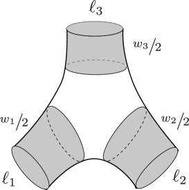
Figure 3: Hyperbolic pants with the half-collars associated with the boundary geodesics. When $\ell_{1}=\ell_{2}=\ell_{3}=L<L_{*}$ the half collars shown are all of length greater than $L/2$.

4 Hyperbolic string vertices

In this section we introduce a set of hyperbolic string vertices and demonstrate that they provide an exact solution of the master equation (1.1). We also describe in some detail the simplest vertex ${\cal V}_{0,3}$, corresponding to a sphere with three punctures. We discuss what is entailed in finding a concrete description of the genus one, once-punctured vertex ${\cal V}_{1,1}$.

4.1 Hyperbolic vertices as systolic subsets

We first define a subset $\tilde{\cal V}_{g,n}(L)$ of the moduli space ${\cal M}_{g,n,L}$ of genus $g$ surfaces with $n$ boundaries of length $L$:

$$\widetilde{\cal V}_{g,n}(L)\equiv\ \bigl{\{}\ \tilde{\Sigma}\in{\cal M}_{g,n,L}\bigl{|}\ \hbox{sys}(\tilde{\Sigma})\geq L\bigr{\}}\,.$$ (4.1)

Here $\hbox{sys}(\tilde{\Sigma})$ is the systole of $\tilde{\Sigma}$: the length of the shortest non-contractible closed geodesic in $\tilde{\Sigma}$ which is not a boundary component. Since the boundary geodesics have length $L$, the above sets include all surfaces in ${\cal M}_{g,n,L}$ that have no geodesic of length less than $L$. This definition applies for all vertices listed in (1.2), namely $n\geq 3$ for $g=0$, $n\geq 1$ for $g=1$, and $n\geq 0$ for $g\geq 2$. For $n=0$, the space ${\cal M}_{g,0,L}$ is just ${\cal M}_{g,0}$.

The string vertices ${\cal V}_{g,n}(L)$ are now obtained by applying $\hbox{gr}^{\prime}_{\infty}$ to the above sets, namely, by grafting the semi-infinite cylinders to turn the boundaries into punctures with local coordinates:

$${\cal V}_{g,n}(L)\equiv\hbox{gr}^{\prime}_{\infty}\,\bigl{(}\widetilde{\cal V}_{g,n}(L)\bigr{)}\,.$$ (4.2)

Theorem 1: The sets ${\cal V}_{g,n}(L)$ with $L\leq L_{*}$ solve the master equation (1.1).

Proof. We must now show that the above string vertices, defining ${\cal V}$ as the formal sum (1.2), solve the equation:

$$\partial{\cal V}=-\hbar\Delta{\cal V}-\tfrac{1}{2}\{{\cal V}\,,{\cal V}\}\,.$$ (4.3)

We first show that the surfaces appearing in the boundary of ${\cal V}$ are contained on the right-hand side. The boundary of ${\cal V}$ arises when a simple closed interior geodesic becomes of length $L$. The geodesic cannot be non-simple since all such geodesics are at least of length $2L_{*}$ (see [22], Theorem 4.2.2). Note that two intersecting closed geodesics cannot reach length $L$ simultaneously either because of Claim 1. When more than one simple closed geodesic becomes of length $L$ we are simply at a lower codimension set on the boundary.

Suppose we cut the surface $S$ at the length $L$ geodesic, obtaining the surface $S_{c}$. Then either $S_{c}$ is two disconnected surfaces, or $S_{c}$ remains connected. If $S_{c}$ is disconnected each surface is in a string vertex, for none has a geodesic shorter than $L$, and all boundaries are geodesics of length $L$. Then $S$ arises from $\{{\cal V}\,,{\cal V}\}$. If $S_{c}$ remains connected, $S_{c}$ has two more boundaries than $S$, and is contained in a string vertex, having no geodesic shorter than $L$ and boundaries of length $L$. Then $S$ arises from $\Delta$ acting on $S_{c}$. This proves that the boundary of ${\cal V}$ is indeed contained on the right-hand side.

Now we must show that the sewing operations on the right-hand side of (4.3) acting on surfaces belonging to string vertices give us surfaces on the boundary of the string vertices. Consider first the case when we sew together boundary geodesics on two separate surfaces $S_{1}$ and $S_{2}$, each from a string vertex.

At the seam the new surface has a geodesic of length exactly $L$. The new surface must be checked to have systole $L$. No geodesic totally contained in $S_{1}$ or in $S_{2}$ is shorter than $L$, so the only concern is that a geodesic $\gamma$ that runs on both surfaces is shorter than $L$. Such curve would have to intersect the simple closed curve at the seam but this is impossible due to Claim 1.

In fact, the condition $L\leq L_{*}$ used for Claim 1 is not needed for these curves to work out. Any short geodesic $\gamma$ running on both surfaces has a piece of length $\ell_{1}$ in $S_{1}$ and a piece of length $\ell_{2}$ in $S_{2}$, with $\ell_{1}+\ell_{2}<L$. The geodesic cuts the seam into two pieces of length $a_{1}$ and $a_{2}$ with $a_{1}+a_{2}=L$. At least one of $\ell_{1},\ell_{2}$, call it $\ell_{i}$, must be smaller than $L/2$. And at least one of $a_{1},a_{2}$, call it $a_{j}$, satisfies $a_{j}\leq L/2$. The closed curve $\tilde{\gamma}$ formed by $\ell_{i}$ followed by $a_{j}$ would be smaller than $L$ and would be contained in $S_{i}$. Moreover $\tilde{\gamma}$ is a non-contractible curve, because otherwise, $\gamma$ itself would be homotopic to a curve in just one of the two surfaces. In summary, $\tilde{\gamma}$ is a non-contractible closed curve on $S_{i}$ that is shorter than $L$. This is impossible, and proves the claim.

If we sew two boundary geodesics on a single surface belonging to a string vertex, we create a new handle with a geodesic of length $L$ along the seam. Any new potentially short curve must traverse this collar and intersect the seam, which is ruled out by Claim 1. Thus the surfaces on the right-hand side of (4.3) are in $\partial{\cal V}$. In this case the collar was required. This concludes the proof that the chosen string vertices satisfy the geometric master equation. $\square$

Comments:

1. Since the map $\hbox{gr}_{\infty}:{\cal M}_{g,n,L}\to{\cal M}_{g,n}$ is a homeomorphism it follows that the string vertices define a piece of a section over the moduli space ${\cal M}_{g,n}$.

2. The vertices cover what is usually called the ‘thick’ part of the moduli space, the part including all surfaces with systole greater than or equal to some positive number $\epsilon$. The vertices are a compact subset of moduli space, by Mumford’s compactness criterion [27].

3. All string vertices are non-empty sets. This is nontrivial: for a choice of $L$ the systole is a function on ${\cal M}_{g,n,L}$ that is bounded above. Over the moduli space ${\cal M}_{2,0}$, for example, the systole has a maximum at the Bolza surface with value $2\,\hbox{arccosh}(1+\sqrt{2})\simeq 3.057$ [28, 29]. This surface would be included in any ${\cal V}_{2,0}(L)$ since $L\leq L_{*}\simeq 1.7628$.

4.2 The three-string vertex

The lowest-dimensional subset in ${\cal V}$ is ${\cal V}_{0,3}(L)$. This subset includes one surface, a sphere with three punctures. By definition, $\tilde{\cal V}_{0,3}(L)$ is the hyperbolic pants with three geodesic boundaries all of length $L$. There is just one surface in the corresponding moduli space. To this surface we again attach semi-infinite cylinders to obtain ${\cal V}_{0,3}(L)$ (see Figure 4).

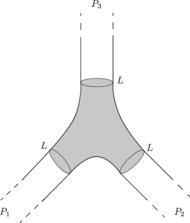
Figure 4: The surface ${\cal V}_{0,3}(L)$ is the three-punctured sphere obtained by attaching three semi-infinite cylinders of circumference $L$ to the geodesic boundaries of the symmetric hyperbolic pants with boundary lengths all set equal to $L$.

The symmetric pants with boundaries of length $L$ is constructed from gluing two copies of a geodesic hexagon with sides lengths $\tfrac{L}{2},\gamma,\tfrac{L}{2},\gamma,\tfrac{L}{2},\gamma$, as shown in Figure 5. The length $\gamma$ is the geodesic length between any pair of boundaries.

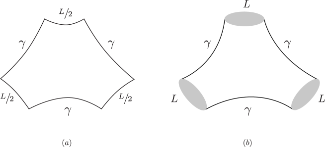
Figure 5: (a) A hexagon with geodesic edges that meet orthogonally at each vertex. This is a special vertex with three edges of length $L/2$ and three edges of length $\gamma$. (b) Gluing two such hexagons across the length $\gamma$ edges we obtain a pants diagram, the string vertex with three equal boundaries that are geodesics of length $L$.

Hexagon identities (see [22], Theorem 2.4.1) tell us that $\gamma$ is given by

$$\cosh\gamma={\cosh\tfrac{L}{2}\over\cosh\tfrac{L}{2}-1}\,.$$ (4.4)

This shows that as $L\to\infty$, the distance $\gamma$ between geodesic boundaries goes to zero: $\gamma\simeq 2e^{-L/4}$. This is as expected because the area $A_{0,3}$ of the surface is fixed. In fact, from Gauss Bonnet we have $A_{g,b}=2\pi(2g-2+b)$ with $g$ and $b$ the genus and the number of boundaries. This gives $A_{0,3}=2\pi$ for the hyperbolic ${\cal V}_{0,3}(L)$, independent of the value of $L$. With the area fixed and the boundaries becoming infinitely long, the distance between the boundaries is going to zero.

To become more familiar with the hyperbolic vertex we consider ${\cal V}_{0,3}(L_{*})$, the vertex for the largest possible value of $L$. In this case $\cosh\tfrac{L*}{2}=\sqrt{2}$ and $\gamma_{*}$ is readily determined:

$$\cosh\gamma_{*}=2+\sqrt{2}\,,\quad\gamma_{*}=\log\Bigl{(}2+\sqrt{2}+\sqrt{5+4\sqrt{2}}\,\Bigr{)}\simeq 1.89892\,.$$ (4.5)

Since the collar width $w_{*}=L_{*}\simeq 1.76275<\gamma_{*}$, the half collars around the boundary geodesics, each of width $w_{*}/2$, do not touch. This is as it should. The vertex ${\cal V}_{0,3}(L_{*})$ is built by gluing two hexagons, each of sides $\tfrac{L_{*}}{2},\gamma_{*},\tfrac{L_{*}}{2},\gamma_{*},\tfrac{L_{*}}{2},\gamma_{*}$. Each hexagon can be displayed in the upper half-plane $\mathbb{H}$, with standard metric $ds=|dz|/y$. We do this in Figure 6. The construction follows the method used to show that hyperbolic hexagons with prescribed lengths for three non-consecutive edges exist (see [22], Section 1.7). Two of the sides of length $L_{*}/2$ appear as the arcs from the imaginary axis to the line $B$, that has slope one. There is a circle centered at $\sqrt{2}$ with radius one, and a circle at $x_{c}$ with radius $r_{c}$, given by

$$x_{c}={1\over 4}\Bigl{(}2+3\sqrt{2}+\sqrt{2}\sqrt{5+4\sqrt{2}}\ \Bigr{)}\simeq 2.715\,,\quad r_{c}^{2}={1\over 2}\sqrt{\sqrt{2}+\sqrt{2\sqrt{2}-1}\ }\ \simeq 0.8316\,.$$ (4.6)

The vertical edge runs from $i$ to $ie^{\gamma_{*}}\simeq i\,6.679$. There is a circle centered at $\sqrt{2}e^{\gamma_{*}}\simeq 9.445$ with radius $e^{\gamma_{*}}$; its intersection with the real axis is close but does not coincide with $x_{c}$.

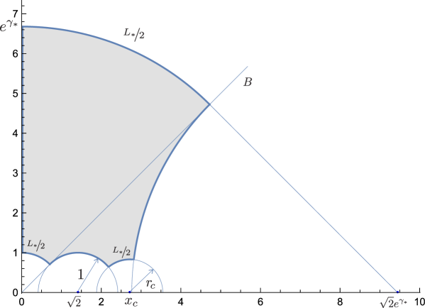
Figure 6: The hyperbolic vertex ${\cal V}_{0,3}(L_{*})$ is constructed by gluing together two hyperbolic hexagons with alternating edges $L_{*}$ and $\gamma_{*}$ across the $\gamma_{*}$ edges. The hyperbolic hexagon is shown above, as the shaded area. The line $B$ is at exactly at $\pi/4$ angle, and the circular arcs from the imaginary axis to $B$ are two sides of length $L_{*}/2$. All other sides are of length $\gamma_{*}$.

Comments on the vertex ${\cal V}_{1,1}(L)$.

We wish to illustrate what is involved in giving an explicit construction of the systolic set ${\cal V}_{1,1}(L)$. We begin with the Teichmüller space ${\cal T}_{1,1,L}$ of genus one surfaces with one geodesic boundary of length $L$. This space can be described with Fenchel-Nielsen coordinates. We take a set of pants with boundary lengths $L,L^{\prime},L^{\prime}$ and glue the length-$L^{\prime}$ boundaries together with twist parameter $\alpha$. As $L^{\prime}\in[0,\infty]$ and $\alpha\in(-\infty,\infty)$, the full space ${\cal T}_{1,1,L}$ is generated.

Two conditions select the subset ${\cal V}_{1,1}(L)$: systole $L$ and restriction to inequivalent surfaces under the action of the mapping class group. Since surfaces with $\alpha$ and $\alpha+1$ are the same Riemann surface, we can restrict ourselves to $\alpha\in[0,1]$. Moreover, since $L^{\prime}$ is the length of a nontrivial closed geodesic, so we must take $L^{\prime}>L$. This, however, does not guarantee that the systole is $L$; other geodesics can become short. In particular, when $\alpha={1\over 2}$ (the case when gluing turns the geodesic between the two length-$L^{\prime}$ boundaries into a closed geodesic) and $L^{\prime}$ is large, there is a geodesic shorter than $L$. The systolic condition defines a nontrivial subregion in the space $L^{\prime}>L,\alpha\in[0,1]$. Within this region, one must determine the set of inequivalent surfaces. This is challenging since the mapping class group does not have a simple action on Fenchel-Nielsen coordinates.

5 The Feynman region

In this section we consider the Feynman diagrams formed with the hyperbolic string vertices defined in section 4. We will explain how the obvious metric on the Riemann surfaces is hyperbolic at the vertices and flat on the cylinders that represent the propagators. We discuss the mathematical framework relevant to these Thurston metrics. This is the theory of complex projective structures and measured laminations, which suggests these metrics are rather natural (for a review of these topics see [32]). We are unable to determine if the Feynman graphs provide a section of $\widehat{\cal P}_{g,n}$ over ${\cal M}_{g,n}$ but discuss partial results in the literature that indicate the affirmative answer is quite plausible.

When the vertices are glued directly across length $L$ boundaries the resulting surface remains hyperbolic; that was in fact a requirement for the vertices to satisfy the master equation. If a propagator is added, however, an annulus is grafted: the boundaries of the annulus are attached to boundaries on the surfaces (on two different surfaces or on the same surface). Once we insert the annulus there is no direct way to get a hyperbolic metric on the whole surface. If we put a hyperbolic metric on the annulus, the total metric is discontinuous at the seams, thus not hyperbolic. The string field theory indicates that the cylinder, of circumference $L$ must be added with all values $t>0$ of the height, and with all values $0\leq\theta<2\pi$ of the twist angle $\theta$. This range of the twist takes into account that in moduli space we get the same surface for $\theta=0$ and $\theta=2\pi$. In the Feynman region we generally include several propagators, so we will have a collection $(t_{i},\theta_{i})$ of parameters, with $i=1,\cdots,N_{p}$, with $N_{p}$ the number of propagators.

In string field theory it is natural to introduce such annuli as finite-length flat cylinders of circumference $L$ that are grafted into the surface. In this way the metric on the whole surface is partially hyperbolic on the vertices and flat on the grafting cylinders (Figure 7). The metric is $C^{1}$ continuous but not smooth: the curvature changes discontinuously across seams from $K=-1$ on the hyperbolic part to $K=0$ on the cylinder. This metric is called a Thurston metric on the surface, and arises naturally through an intrinsic definition [34] reviewed below.

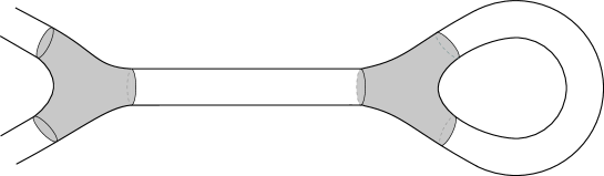
Figure 7: A Feynman diagram gives Riemann surfaces with metrics that are hyperbolic on the string vertices (shown shaded) and flat on the propagators.

To begin, consider a complex projective $\mathbb{CP}^{1}$ structure on a compact surface $S$: an atlas of charts valued on $\mathbb{CP}^{1}$ with Möbius transition functions. We call ${\cal P}(S)$ the set of (isotopy classes of) marked complex projective structures. Since Möbius maps are holomorphic there is a projection map to Teichmüller space $\pi:{\cal P}(S)\to{\cal T}(S)$. It is known that one can identify ${\cal P}(S)$ with the bundle ${\cal Q}(S)\to{\cal T}(S)$ of quadratic differentials over Teichmüller space.

An alternative description of ${\cal P}(S)$ was given by Thurston. Consider a hyperbolic surface $X\in{\cal T}(S)$ (a Riemann surface) and a simple closed geodesic $\gamma$. Cut the surface at $\gamma$ and graft a flat cylinder $\gamma\times[0,t]$ of height $t$. The result is the surface $\hbox{Gr}_{t\gamma}X$. In fact $\hbox{Gr}_{t\gamma}X$ has a canonical projective structure provided by the Fuchsian uniformization of $X$ and the Euclidean structure on the cylinder. A simple closed geodesic on a hyperbolic surface with a weight $t$ is the simplest example of a measured geodesic lamination $\lambda=t\gamma$ on the surface. A more general measured geodesic lamination $\lambda$ is a collection of non-intersecting simple closed geodesics $\gamma_{i}$ each one with a weight $t_{i}$. We then have

$$\lambda=\sum t_{i}\gamma_{i}\,.$$ (5.1)

Grafting places a cylinder $\gamma_{i}\times[0,t_{i}]$ on each geodesic $\gamma_{i}$ resulting in a new surface with a projective structure.

Thurston showed that grafting, yielding a projective structure, can be defined more generally on the space ${\cal ML}(S)$ of measured geodesic laminations. In fact one has a map

$$\hbox{Gr:}\ {\cal ML}(S)\times{\cal T}(S)\to{\cal P}(S)\,.$$ (5.2)

If we pick a surface $X\in{\cal T}(S)$ and a lamination $\lambda\in{\cal ML}(S)$ then $\hbox{Gr}_{\lambda}X$ is the projective structure we obtain, and we call $\hbox{gr}_{\lambda}X$ the conformal structure underlying the projective structure.

Given a Riemann surface $\Sigma$, that is, a complex structure, the surface admits a unique hyperbolic structure. But there are infinitely many projective structures on $\Sigma$. The metric that characterizes a projective structure is the Thurston metric. To define it, consider first a unit disk $D=\{z\in\mathbb{C},|z|<1\}$ and let $\rho_{D}$ denote the hyperbolic metric on $D$. Now, let $R$ denote a $\mathbb{CP}^{1}$ manifold, $x\in R$ denote a point, and $v\in T_{x}R$ a vector. The Thurston metric $t_{R}$ assigns to the vector $v$ the length $t_{R}(v)$ given by

$$t_{R}(v)=:\inf_{f:D\to R}\rho_{D}(f^{*}v)\,,$$ (5.3)

with the infinimum evaluated over all projective immersions $f:D\to R$ for which $x\in f(D)$. This definition is analogous to the definition of the Kobayashi metric on a Riemann surface, in which case the immersions $f$ are holomorphic and the resulting Kobayashi metric coincides with the hyperbolic metric. The Thurston metric for the projective structure $Gr_{\lambda}X$ has been shown to be the mixed metric: hyperbolic on the vertices and flat on the cylinders.

Now let us examine the question of sections in the bundle $\widehat{\cal P}_{g,n}$ over ${\cal M}_{g,n}$. A useful result by Dumas and Wolf [25] (Theorem 1.1) tells us that for any $X\in{\cal T}(S)$ and any lamination $\lambda\in{\cal ML}(S)$, the grafting map $\hbox{gr}_{\lambda}X$ is a homeomorphism from ${\cal ML}(S)\to{\cal T}(S)$. Consider now our construction of Feynman graphs with $(t_{i},\theta_{i})$ parameters with fixed $\theta_{i}$. We can implement all the twists before grafting, by cutting open the geodesics and twisting. Then we graft with cylinders of circumference $L$ and heights $t_{1},\cdots,t_{N_{p}}\in[0,\infty)$. Since the heights are the parameters of a measured lamination, this shows that the parameter space of heights (with fixed twists) is mapped injectively into Teichmüller space. It is not a priori guaranteed to be an injective map into moduli space but it is locally injective and, since it approaches infinity in moduli space, the map is at most finite to one.

This is encouraging, but not sufficient as we would like to have an injective map of the full parameter space of heights and twists into Teichmüller space and then into moduli space. The case of heights and twists together has been considered by McMullen [35], who’s views it as a “complex earthquake” and shows that at least in the case of a punctured torus, it provides a homeomorphism to Teichmüller space. It seems likely that for large heights the map from the Feynman parameters to moduli space is in fact injective: for long cylinders the length/twist coordinates approach the standard plumbing coordinates used to describe degeneration.

An injective map to moduli space is not always obtained when grafting with heights $[0,\infty]$ and twists $[0,2\pi]$ on arbitrary geodesics. In our case, if we get an injective map from the full Feynman parameter space into moduli space, it must be because the vertices are hyperbolic surfaces in systolic sets. We think it is likely that the Feynman rules construct sections.

A decomposition of moduli space ? If the Feynman rules produce a section of $\widehat{\cal P}_{g,n}$ over ${\cal M}_{g,n}$ the various Feynman diagrams define a decomposition of ${\cal M}_{g,n}$:

$${\cal M}_{g,n}={\cal V}_{g,n}\cup R_{1}\cup\ \cdots\cup R_{3g-3+n}\,,$$ (5.4)

where $R_{k}$ denotes the set of surfaces generated by a Feynman diagram with $k$ propagators. If we have a section, the sets on the right-hand side are disjoint, except at boundaries, and together built the moduli space. The geometric master equation implies that the right-hand side builds a space whose only boundary is the boundary of moduli space.

We can think of ${\cal V}_{g,n}$ as a graph with just a vertex and $n$ external lines. It is an $(6g-6+2n)$ real-dimensional subset of ${\cal M}_{g,n}$, representing the ‘thick’ part of the moduli space. In $R_{1}$ we have one propagator, representing grafting with parameters $(t,\theta)$ with $t\in[0,\infty),\theta\in[0,2\pi)$. Points in $R_{1}$ arise in two possible ways. We may have two surfaces grafted together: one in ${\cal V}_{g_{1},n_{1}}$ the other in ${\cal V}_{g_{2},n_{2}}$ with $g_{1}+g_{2}=g,\,n_{1}+n_{2}=n+2$, in which case the graph is one with two vertices and one edge, as well as $n$ external lines. One can also have a surface in ${\cal V}_{g-1,n+2}$ with two boundaries grafted by the propagator, in which case the graph has one vertex, one edge starting and ending on the vertex, and $n$ external lines. In both cases the assumption of a section implies that the space of grafting parameters and vertex parameters is mapped injectively into moduli space.

Each diagram in $R_{3g-3+n}$ is built with $(2g-2+n)$ hyperbolic vertices ${\cal V}_{0,3}$ (having no parameters) and $(3g-3+n)$ propagators, assembled together with the instruction of a connected cubic graph. One must then sum over all possible inequivalent graphs. If we have a section, this construction maps the full parameter space of heights and twists of each diagram injectively into the moduli space ${\cal M}_{g,n}$ of genus $g$ surfaces. Each diagram builds a different region of ${\cal M}_{g,n}$. The heights and twists, $(3g-3+n)$ of each, provide coordinates on the part of the moduli space they produce.

This is quite different from the way Fenchel-Nielsen coordinates work. In this case a single connected cubic graph with $(2g-2+n)$ vertices is used to glue together hyperbolic pants. The length and twist coordinates are encoded on the $(3g-3+2n)$ edges of the graph, each one representing a seam. As these parameters run over their usual ranges (zero to infinity for length and minus to plus infinity for twist) one has a homeomorphism to Teichmüller space. One need not sum over graphs. In the string motivated construction, one sums over all cubic graphs with fixed hyperbolic pants and the coordinates arise from grafting.

6 Comments and open questions

We begin with some comments and elaborations on our results.

1. This proposal seems to give the first rigorous explicit construction of string vertices. In [13, 14] some aspects of the construction can only be made explicit in approximations. The systolic minimal area metrics, despite recent progress, have not yet been rigorously proven to exist in the thick parts of the higher-genus moduli spaces.

2. A particularly elegant property of the hyperbolic vertices is that they come naturally with collars that prevent the creation of short curves when vertices are glued together. In the minimal area approach, one must retract the obvious local coordinates by the addition of stubs in order to prevent this from happening.

3. While the construction of the quantum theory requires $L\leq L_{*}$, the classical hyperbolic closed string field theory works with arbitrary $L>0$. That is, if we restrict the string vertices to the genus zero contributions ${\cal V}=\sum_{n=3}^{\infty}\,{\cal V}_{0,n}$, we get a solution of the classical master equation

   $$\partial{\cal V}+\tfrac{1}{2}\{{\cal V}\,,{\cal V}\}=0\,,$$ (6.1)

   for any $L>0$. This solution works for $L>L^{*}$ because, as discussed in the proof of Theorem 1 in section 4, no non-contractible curve shorter than $L$ is created by the gluing of two separate surfaces belonging to vertices. While collars become tiny as $L$ grows, collars are not needed in this case.

   In fact since the hyperbolic vertices (viewed as surfaces with boundaries) have finite constant area, as $L\to\infty$ they become like ribbon graphs of vanishing width. In this limit the surfaces with infinite cylinders attached, and rescaled by $2\pi/L$, become the minimal area vertices of closed string field theory. The surface acquires a Strebel differential whose critical graph is a restricted polyhedron of classical closed string field theory [36, 37].

4. Open string field theory can also be defined using hyperbolic metrics. Consider the classical theory only. The three open-string vertex would be defined precisely by the hyperbolic hexagon $\tfrac{L}{2},\gamma,\tfrac{L}{2},\gamma,\tfrac{L}{2},\gamma$, shown in Figure 5(a) and in Figure 6 for the case $L=L_{*}$. The external open strings are now three semi-infinite strips of width $L/2$ attached to the three sides of length $L/2$. The open string boundary conditions apply to the three $\gamma$ edges. This hexagon diagram is obtained by cutting the pants ${\cal V}_{0,3}$ across a line invariant under an antiholomorphic involution. In fact ${\cal V}_{0,3}$ was defined by the gluing of two hexagons. The hyperbolic open string vertex does not satisfy strict associativity and therefore hyperbolic classical hyperbolic open string field theory is a non-polynomial theory organized by an $A_{\infty}$ algebra  [38]. It has vertices with $n\geq 4$ open strings. These vertices can be obtained from the closed string vertices ${\cal V}_{0,n}$ by selecting the surfaces with antiholomorphic involution and cutting.

We end with a discussion of some open questions that seem relevant to us.

1. Proving that the hyperbolic string theory generates a section in the $\widehat{\cal P}_{g,n}$ bundle over ${\cal M}_{g,n}$. This may require extending the theory of complex earthquakes. An alternative approach would involve devising a convex minimization problem on a Riemann surface with punctures whose then unique answer is the metric built with the string field theory that uses the hyperbolic vertices.

2. Developing the tools to compute string amplitudes in this framework. The first calculation would be to compute three-point functions using the three-string vertex. Presumably the simplest approach would be to develop the theory is holomorphic objects on the 3-holed sphere. The operator formulation of the conformal field theory would then yield the required amplitudes.

3. The full quantum action is written in terms of the vertices that are systolic subsets of moduli spaces with hyperbolic metrics. Perhaps the evaluation of integrals over these sets can be performed using the associated Teichmuller spaces, in the spirit of [15, 17, 39] and along the lines discussed in [14].

4. Finding coordinates to describe the systolic sets that define the string vertices. If point one above is true, then these coordinates together with the propagator parameters $(t_{i},\theta_{i})$ would give coordinates all over moduli space.

5. It’s difficult to think about hyperbolic metrics on an $N=1$ super Riemann surface, but the key ideas used here can expressed in purely group-theoretical terms. The symmetry of the universal cover is $\hbox{SL}(2,R)$ and there is map from the fundamental group to $\hbox{SL}(2,R)$. The length of the geodesic in a particular class in the fundamental group can be read off the corresponding conjugacy class in $\hbox{SL}(2,R)$. There are uniformization theorems for $N=1$ super Riemann surfaces [40] and the symmetry group of the universal cover is some supergroup. While we can’t really talk about the length of a hyperbolic geodesic super Riemann surface, we can look at the conjugacy class in this super-group as a replacement.

Acknowledgements

We are very grateful for instructive and detailed correspondence with Jørgen Andersen, David Dumas, Gabriele Mondello, Michael Wolf, and Scott Wolpert.

We acknowledge the hospitality of the Simons Center for Geometry and Physics for the workshop ‘String field theory, BV quantization, and moduli spaces’ (May 20-24, 2019), where this research was started.

K.C. is supported by the Krembil Foundation, the NSERC Discovery Grant program and by the Perimeter Institute for Theoretical Physics. Research at Perimeter Institute is supported by the Government of Canada through Industry Canada and by the Province of Ontario through the Ministry of Research and Innovation. B.Z is partially supported by the U.S. Department of Energy, Office of Science, Office of High Energy Physics of U.S. Department of Energy under grant Contract Number DE-SC0012567.

References

- [1] B. Zwiebach, “Closed string field theory: Quantum action and the B-V master equation,” Nucl. Phys. B 390, 33 (1993) doi:10.1016/0550-3213(93)90388-6 [hep-th/9206084].
- [2] A. Sen, “BV Master Action for Heterotic and Type II String Field Theories,” JHEP 1602, 087 (2016) doi:10.1007/JHEP02(2016)087 [arXiv:1508.05387 [hep-th]].
- [3] C. de Lacroix, H. Erbin, S. P. Kashyap, A. Sen and M. Verma, “Closed Superstring Field Theory and its Applications,” Int. J. Mod. Phys. A 32, no. 28n29, 1730021 (2017) doi:10.1142/S0217751X17300216 [arXiv:1703.06410 [hep-th]].
- [4] A. Sen and B. Zwiebach, “Background independent algebraic structures in closed string field theory,” Commun. Math. Phys. 177, 305 (1996) doi:10.1007/BF02101895 [hep-th/9408053].
- [5] A. Sen and B. Zwiebach, “Quantum background independence of closed string field theory,” Nucl. Phys. B 423, 580 (1994) doi:10.1016/0550-3213(94)90145-7 [hep-th/9311009].
- [6] H. Sonoda and B. Zwiebach, “Closed String Field Theory Loops With Symmetric Factorizable Quadratic Differentials,” Nucl. Phys. B 331, 592 (1990). doi:10.1016/0550-3213(90)90086-S
- [7] K. J. Costello, “The Gromov-Witten potential associated to a TCFT,” [eprint arXiv:math/0509264].
- [8] H. Hata and B. Zwiebach, “Developing the covariant Batalin-Vilkovisky approach to string theory,” Annals Phys. 229, 177 (1994) doi:10.1006/aphy.1994.1006 [hep-th/9301097].
- [9] B. Zwiebach, “How covariant closed string theory solves a minimal-area problem,” Commun. Math. Phys. 136, 83 (1991). doi:10.1007/BF02096792
- [10] M. Headrick and B. Zwiebach, “Convex programs for minimal-area problems,” arXiv:1806.00449 [hep-th].
- [11] M. Headrick and B. Zwiebach, “Minimal-area metrics on the Swiss cross and punctured torus,” arXiv:1806.00450 [hep-th].
- [12] U. Naseer and B. Zwiebach, “Extremal isosystolic metrics with multiple bands of crossing geodesics,” arXiv:1903.11755 [math.DG].
- [13] S. F. Moosavian and R. Pius, “Hyperbolic Geometry and Closed Bosonic String Field Theory I: The String Vertices Via Hyperbolic Riemann Surfaces,” arXiv:1706.07366 [hep-th].
- [14] S. F. Moosavian and R. Pius, “Hyperbolic Geometry and Closed Bosonic String Field Theory II: The Rules for Evaluating the Quantum BV Master Action,” arXiv:1708.04977 [hep-th].
- [15] G. McShane, “Simple geodesics and a series constant over Teichmuller space,” Inventiones mathematicae 132.3 (1998): 607-632.
- [16] M. Mirzakhani, “Simple geodesics and Weil-Petersson volumes of moduli spaces of bordered Riemann surfaces”, Invent. Math. 167, no. 1, 179 (2006). doi:10.1007/s00222-006-0013-2
- [17] M. Mirzakhani, “Weil-Petersson volumes and intersection theory on the moduli space of curves,” J. Am. Math. Soc. 20, no. 01, 1 (2007). doi:10.1090/S0894-0347-06-00526-1.
- [18] R. Dijkgraaf and E. Witten, “Developments in Topological Gravity,” Int. J. Mod. Phys. A 33, no. 30, 1830029 (2018) doi:10.1142/S0217751X18300296 [arXiv:1804.03275 [hep-th]].
- [19] S. A. Wolpert, “The hyperbolic metric and the geometry of the universal curve,” J. Differential Geometry 31 (1990) 417-472.
- [20] K. Obitsu and S. A. Wolpert, “Grafting hyperbolic metrics and Eisenstein series,” Math. Ann. 341 (2008), no. 3, 685-706. MR 2399166 (2009d:32011) [arXiv:0704.3169]
- [21] K. Costello, unpublished, announced at the Simons Center Workshop on String field theory, BV quantization and moduli spaces (May 20-24, 2019).
- [22] P. Buser, “Geometry and spectra of compact Riemann surfaces,” Birkhäuser Boston 1992.
- [23] G. Mondello, “Riemann surfaces with boundary and natural triangulations of the Teichmüller space,” J. Eur. Math. Soc. (JEMS) 13 (2011), pp. 635-684 [eprint arXiv:0804.0605].
- [24] S. F. Moosavian and Y. Zhou, “On the existence and uniqueness of closed-superstring field theory vertices”, to appear.
- [25] D. Dumas and M. Wolf, “Projective structures, grafting and measured laminations,” Geometry & Topology 12 (2008) 351-386 [eprint arXiv:0712.0968].
- [26] J. E. Andersen, talk at ‘Resurgence in Mathematics and Physics’, (11-14 June 2019) IHES, Le Bois-Marie.
- [27] D. Mumford, “A remark on Mahler’s compactness theorem,” Proc. Amer. Math. Soc. 28 (1971), 289-294.
- [28] F. Jenni, Comment. Math. Helv., 59(2):193-203, 1984.
- [29] H. Parlier, “Simple closed geodesics and the study of Teichmüller spaces,” Handbook of Teichmüller theory. Vol. IV, IRMA Lect. Math. Theor. Phys., vol. 19, Eur. Math. Soc., Zurich, 2014, pp. 113-134 [arXiv:0912.1540]
- [30] J. H. Hubbard, “ Teichmüller Theory and Applications to Geometry, Topology, and Dynamics.” Matrix Editions (2006).
- [31] L. Keen, “On fundamental domains and the Teichmüller modular group,” in Contributions to Analysis, a collection of papers dedicated to Lipman Bers (I. V. Ahlfors et al., eds), Academic Press, London-New York-San Francisco (1974) 185-194.
- [32] D. Dumas, ‘Survey: Complex projective structures.’ In Handbook of Teichm ller Theory, Volume II. Ed. Athanase Papadopoulos. EMS, 2009. doi:10.4171/055
- [33] K. P. Scannell and M. Wolf, “The grafting map of Teichmüller space.” J. Amer. Math. Soc. 15(2002), 893-927 [eprint arXiv:math/9810082].
- [34] H. Tanigawa, “Grafting, harmonic maps and projective structures on surfaces,” J. Differential Geometry 47 (1997) 399-419. [arXiv:math/9508216]
- [35] C. T. McMullen, “Complex earthquakes and Teichmüller theory,” Journal of the American Mathematical Society, Vol. 11, 2, (1998) 283-320.
- [36] T. Kugo, H. Kunitomo and K. Suehiro, “Nonpolynomial Closed String Field Theory,” Phys. Lett. B 226, 48 (1989). doi:10.1016/0370-2693(89)90287-6
- [37] M. Saadi and B. Zwiebach, “Closed String Field Theory from Polyhedra,” Annals Phys. 192, 213 (1989). doi:10.1016/0003-4916(89)90126-7
- [38] M. R. Gaberdiel and B. Zwiebach, “Tensor constructions of open string theories. 1: Foundations,” Nucl. Phys. B 505, 569 (1997) doi:10.1016/S0550-3213(97)00580-4 [hep-th/9705038].
- [39] J. E. Andersen, G. Borot, S. Charbonnier, V. Delecroix, A. Giacchetto, D. Lewanski, C. Wheeler, “Topological recursion for Masur-Veech volumes,” arXiv:1905.10352; J. E. Andersen, G. Borot, and N. Orantin, ‘Geometric Recursion,” eprint arXiv:1711.04729.
- [40] L. Crane and J. M. Rabin, “Superriemann Surfaces: Uniformization and Teichmuller Theory,” Commun. Math. Phys. 113, 601 (1988). doi:10.1007/BF01223239