Adaptively Sparse Transformers

Abstract

Attention mechanisms have become ubiquitous in NLP. Recent architectures, notably the Transformer, learn powerful context-aware word representations through layered, multi-headed attention. The multiple heads learn diverse types of word relationships. However, with standard softmax attention, all attention heads are dense, assigning a non-zero weight to all context words. In this work, we introduce the adaptively sparse Transformer, wherein attention heads have flexible, context-dependent sparsity patterns. This sparsity is accomplished by replacing softmax with $\alpha$-entmax: a differentiable generalization of softmax that allows low-scoring words to receive precisely zero weight. Moreover, we derive a method to automatically learn the $\alpha$ parameter – which controls the shape and sparsity of $\alpha$-entmax – allowing attention heads to choose between focused or spread-out behavior. Our adaptively sparse Transformer improves interpretability and head diversity when compared to softmax Transformers on machine translation datasets. Findings of the quantitative and qualitative analysis of our approach include that heads in different layers learn different sparsity preferences and tend to be more diverse in their attention distributions than softmax Transformers. Furthermore, at no cost in accuracy, sparsity in attention heads helps to uncover different head specializations.

1 Introduction

The Transformer architecture (Vaswani et al., 2017) for deep neural networks has quickly risen to prominence in NLP through its efficiency and performance, leading to improvements in the state of the art of Neural Machine Translation (NMT; Junczys-Dowmunt et al., 2018; Ott et al., 2018), as well as inspiring other powerful general-purpose models like BERT (Devlin et al., 2019) and GPT-2 (Radford et al., 2019). At the heart of the Transformer lie multi-head attention mechanisms: each word is represented by multiple different weighted averages of its relevant context. As suggested by recent works on interpreting attention head roles, separate attention heads may learn to look for various relationships between tokens (Tang et al., 2018; Raganato and Tiedemann, 2018; Mareček and Rosa, 2018; Tenney et al., 2019; Voita et al., 2019).

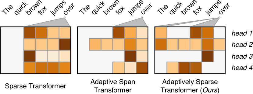
Figure 1: Attention distributions of different self-attention heads for the time step of the token “over”, shown to compare our model to other related work. While the sparse Transformer (Child et al., 2019) and the adaptive span Transformer (Sukhbaatar et al., 2019) only attend to words within a contiguous span of the past tokens, our model is not only able to obtain different and not necessarily contiguous sparsity patterns for each attention head, but is also able to tune its support over which tokens to attend adaptively.

The attention distribution of each head is predicted typically using the softmax normalizing transform. As a result, all context words have non-zero attention weight. Recent work on single attention architectures suggest that using sparse normalizing transforms in attention mechanisms such as sparsemax – which can yield exactly zero probabilities for irrelevant words – may improve performance and interpretability (Malaviya et al., 2018; Deng et al., 2018; Peters et al., 2019). Qualitative analysis of attention heads (Vaswani et al., 2017, Figure 5) suggests that, depending on what phenomena they capture, heads tend to favor flatter or more peaked distributions.

Recent works have proposed sparse Transformers (Child et al., 2019) and adaptive span Transformers (Sukhbaatar et al., 2019). However, the “sparsity” of those models only limits the attention to a contiguous span of past tokens, while in this work we propose a highly adaptive Transformer model that is capable of attending to a sparse set of words that are not necessarily contiguous. Figure 1 shows the relationship of these methods with ours.

Our contributions are the following:

• We introduce sparse attention into the Transformer architecture, showing that it eases interpretability and leads to slight accuracy gains.

• We propose an adaptive version of sparse attention, where the shape of each attention head is learnable and can vary continuously and dynamically between the dense limit case of softmax and the sparse, piecewise-linear sparsemax case.

• We make an extensive analysis of the added interpretability of these models, identifying both crisper examples of attention head behavior observed in previous work, as well as novel behaviors unraveled thanks to the sparsity and adaptivity of our proposed model.

2 Background

2.1 The Transformer

In NMT, the Transformer (Vaswani et al., 2017) is a sequence-to-sequence (seq2seq) model which maps an input sequence to an output sequence through hierarchical multi-head attention mechanisms, yielding a dynamic, context-dependent strategy for propagating information within and across sentences. It contrasts with previous seq2seq models, which usually rely either on costly gated recurrent operations (often LSTMs: Bahdanau et al., 2015; Luong et al., 2015) or static convolutions (Gehring et al., 2017).

Given $n$ query contexts and $m$ sequence items under consideration, attention mechanisms compute, for each query, a weighted representation of the items. The particular attention mechanism used in Vaswani et al. (2017) is called scaled dot-product attention, and it is computed in the following way:

$$\operatorname{\mathsf{Att}}(\bm{Q},\bm{K},\bm{V})=\bm{\pi}\left(\frac{\bm{Q}\bm{K}^{\top}}{\sqrt{d}}\right)\bm{V},$$ (1)

where $\bm{Q}\in\mathbb{R}^{n\times d}$ contains representations of the queries, $\bm{K},\bm{V}\in\mathbb{R}^{m\times d}$ are the keys and values of the items attended over, and $d$ is the dimensionality of these representations. The $\bm{\pi}$ mapping normalizes row-wise using softmax, $\bm{\pi}(\bm{Z})_{ij}=\operatorname*{\mathsf{softmax}}(\bm{z}_{i})_{j}$, where

$$\operatorname*{\mathsf{softmax}}(\bm{z})=\frac{\exp(z_{j})}{\sum_{j^{\prime}}\exp(z_{j^{\prime}})}.$$ (2)

In words, the keys are used to compute a relevance score between each item and query. Then, normalized attention weights are computed using softmax, and these are used to weight the values of each item at each query context.

However, for complex tasks, different parts of a sequence may be relevant in different ways, motivating multi-head attention in Transformers. This is simply the application of Equation 1 in parallel $H$ times, each with a different, learned linear transformation that allows specialization:

$$\operatorname{\mathsf{Head}}_{i}(\bm{Q}\!,\!\bm{K}\!,\!\bm{V})\!=\!\operatorname{\mathsf{Att}}(\bm{QW}_{i}^{Q}\!\!,\bm{KW}_{i}^{K}\!\!,\bm{VW}_{i}^{V}\!)$$ (3)

In the Transformer, there are three separate multi-head attention mechanisms for distinct purposes:

• Encoder self-attention: builds rich, layered representations of each input word, by attending on the entire input sentence.

• Context attention: selects a representative weighted average of the encodings of the input words, at each time step of the decoder.

• Decoder self-attention: attends over the partial output sentence fragment produced so far.

Together, these mechanisms enable the contextualized flow of information between the input sentence and the sequential decoder.

2.2 Sparse Attention

The softmax mapping (Equation 2) is elementwise proportional to $\exp$, therefore it can never assign a weight of exactly zero. Thus, unnecessary items are still taken into consideration to some extent. Since its output sums to one, this invariably means less weight is assigned to the relevant items, potentially harming performance and interpretability (Jain and Wallace, 2019). This has motivated a line of research on learning networks with sparse mappings (Martins and Astudillo, 2016; Niculae and Blondel, 2017; Louizos et al., 2018; Shao et al., 2019). We focus on a recently-introduced flexible family of transformations, $\alpha$-entmax (Blondel et al., 2019; Peters et al., 2019), defined as:

$$\mathop{\mathsf{\alpha}\textnormal{-}\mathsf{entmax}}(\bm{z})\coloneqq\operatorname*{\mathsf{argmax}}_{\bm{p}\in\triangle^{d}}\bm{p}^{\top}\bm{z}+\mathsf{H}^{\textsc{T}}_{\alpha}(\bm{p}),$$ (4)

where $\triangle^{d}\coloneqq\{\bm{p}\in\mathbb{R}^{d}:\sum_{i}p_{i}=1\}$ is the probability simplex, and, for $\alpha\geq 1$, $\mathsf{H}^{\textsc{T}}_{\alpha}$ is the Tsallis continuous family of entropies (Tsallis, 1988):

$$\mathsf{H}^{\textsc{T}}_{\alpha}(\bm{p})\!\coloneqq\!\begin{cases}\frac{1}{\alpha(\alpha-1)}\sum_{j}\!\left(p_{j}-p_{j}^{\alpha}\right)\!,&\!\!\!\alpha\neq 1,\\ -\sum_{j}p_{j}\log p_{j},&\!\!\!\alpha=1.\end{cases}$$ (5)

This family contains the well-known Shannon and Gini entropies, corresponding to the cases $\alpha=1$ and $\alpha=2$, respectively.

Equation 4 involves a convex optimization subproblem. Using the definition of $\mathsf{H}^{\textsc{T}}_{\alpha}$, the optimality conditions may be used to derive the following form for the solution (Appendix B.2):

$$\mathop{\mathsf{\alpha}\textnormal{-}\mathsf{entmax}}(\bm{z})=[(\alpha-1){\bm{z}}-\tau\bm{1}]_{+}^{\nicefrac{{1}}{{\alpha-1}}},$$ (6)

where $[\cdot]_{+}$ is the positive part (ReLU) function, $\bm{1}$ denotes the vector of all ones, and $\tau$ – which acts like a threshold – is the Lagrange multiplier corresponding to the $\sum_{i}p_{i}=1$ constraint.

Properties of $\alpha$-entmax.

The appeal of $\alpha$-entmax for attention rests on the following properties. For $\alpha=1$ (i. e., when $\mathsf{H}^{\textsc{T}}_{\alpha}$ becomes the Shannon entropy), it exactly recovers the softmax mapping (We provide a short derivation in Appendix B.3.). For all $\alpha>1$ it permits sparse solutions, in stark contrast to softmax. In particular, for $\alpha=2$, it recovers the sparsemax mapping (Martins and Astudillo, 2016), which is piecewise linear. In-between, as $\alpha$ increases, the mapping continuously gets sparser as its curvature changes.

To compute the value of $\alpha$-entmax, one must find the threshold $\tau$ such that the r. h .s. in Equation 6 sums to one. Blondel et al. (2019) propose a general bisection algorithm. Peters et al. (2019) introduce a faster, exact algorithm for $\alpha=1.5$, and enable using $\mathop{\mathsf{\alpha}\textnormal{-}\mathsf{entmax}}$ with fixed $\alpha$ within a neural network by showing that the $\alpha$-entmax Jacobian w. r .t. $\bm{z}$ for $\bm{p}^{\star}=\mathop{\mathsf{\alpha}\textnormal{-}\mathsf{entmax}}(\bm{z})$ is

$$\frac{\partial\mathop{\mathsf{\alpha}\textnormal{-}\mathsf{entmax}}(\bm{z})}{\partial\bm{z}}=\operatorname*{\mathsf{diag}}(\bm{s})-\frac{1}{\sum_{j}s_{j}}\bm{ss}^{\top},$$ (7)

$$\text{where}\quad s_{i}=\begin{cases}(p_{i}^{\star})^{2-\alpha},&p_{i}^{\star}>0,\\ 0,&p_{i}^{\star}=0.\\ \end{cases}$$

Our work furthers the study of $\alpha$-entmax by providing a derivation of the Jacobian w. r .t. the hyper-parameter $\bm{\alpha}$ (Section 3), thereby allowing the shape and sparsity of the mapping to be learned automatically. This is particularly appealing in the context of multi-head attention mechanisms, where we shall show in Section 5.1 that different heads tend to learn different sparsity behaviors.

3 Adaptively Sparse Transformers
 with $\alpha$-entmax

We now propose a novel Transformer architecture wherein we simply replace softmax with $\alpha$-entmax in the attention heads. Concretely, we replace the row normalization $\bm{\pi}$ in Equation 1 by

$$\bm{\pi}(\bm{Z})_{ij}=\mathop{\mathsf{\alpha}\textnormal{-}\mathsf{entmax}}(\bm{z}_{i})_{j}$$ (8)

This change leads to sparse attention weights, as long as $\alpha>1$; in particular, $\alpha=1.5$ is a sensible starting point (Peters et al., 2019).

Different $\alpha$ per head.

Unlike LSTM-based seq2seq models, where $\alpha$ can be more easily tuned by grid search, in a Transformer, there are many attention heads in multiple layers. Crucial to the power of such models, the different heads capture different linguistic phenomena, some of them isolating important words, others spreading out attention across phrases (Vaswani et al., 2017, Figure 5). This motivates using different, adaptive $\alpha$ values for each attention head, such that some heads may learn to be sparser, and others may become closer to softmax. We propose doing so by treating the $\alpha$ values as neural network parameters, optimized via stochastic gradients along with the other weights.

Derivatives w. r .t. $\alpha$.

In order to optimize $\alpha$ automatically via gradient methods, we must compute the Jacobian of the entmax output w. r .t. $\alpha$. Since entmax is defined through an optimization problem, this is non-trivial and cannot be simply handled through automatic differentiation; it falls within the domain of argmin differentiation, an active research topic in optimization (Gould et al., 2016; Amos and Kolter, 2017).

One of our key contributions is the derivation of a closed-form expression for this Jacobian. The next proposition provides such an expression, enabling entmax layers with adaptive $\alpha$. To the best of our knowledge, ours is the first neural network module that can automatically, continuously vary in shape away from softmax and toward sparse mappings like sparsemax.

Proposition 1.

Let $\bm{p}^{\star}\coloneqq\mathop{\mathsf{\alpha}\textnormal{-}\mathsf{entmax}}(\bm{z})$ be the solution of Equation 4. Denote the distribution $\tilde{p}_{i}\coloneqq\nicefrac{{(p_{i}^{\star})^{2-\alpha}}}{{\sum_{j}(p_{j}^{\star})^{2-\alpha}}}$ and let $h_{i}\coloneqq-p^{\star}_{i}\log p^{\star}_{i}$. The $i$^th component of the Jacobian $\bm{g}\coloneqq\frac{\partial\mathop{\mathsf{\alpha}\textnormal{-}\mathsf{entmax}}(\bm{z})}{\partial\alpha}$ is

$$g_{i}=\begin{cases}\frac{p_{i}^{\star}-\tilde{p}_{i}}{(\alpha-1)^{2}}+\frac{h_{i}-\tilde{p}_{i}\sum_{j}h_{j}}{\alpha-1},&\alpha>1,\\[6.45831pt] \frac{h_{i}\log p_{i}^{\star}-p_{i}^{\star}\sum_{j}h_{j}\log p_{j}^{\star}}{2},&\alpha=1.\end{cases}$$ (9)

The proof uses implicit function differentiation and is given in Appendix C.

Proposition 1 provides the remaining missing piece needed for training adaptively sparse Transformers. In the following section, we evaluate this strategy on neural machine translation, and analyze the behavior of the learned attention heads.

4 Experiments

We apply our adaptively sparse Transformers on four machine translation tasks. For comparison, a natural baseline is the standard Transformer architecture using the softmax transform in its multi-head attention mechanisms. We consider two other model variants in our experiments that make use of different normalizing transformations:

• 1.5-entmax: a Transformer with sparse entmax attention with fixed $\alpha=1.5$ for all heads. This is a novel model, since 1.5-entmax had only been proposed for RNN-based NMT models (Peters et al., 2019), but never in Transformers, where attention modules are not just one single component of the seq2seq model but rather an integral part of all of the model components.

• $\alpha$-entmax: an adaptive Transformer with sparse entmax attention with a different, learned $\alpha_{i,j}^{t}$ for each head.

The adaptive model has an additional scalar parameter per attention head per layer for each of the three attention mechanisms (encoder self-attention, context attention, and decoder self-attention), i. e.,

$$\big{\{}a_{i,j}^{t}\in\mathbb{R}:{} i\in\{1,\dots,L\},j\in\{1,\dots,H\},$$ (10)

$$t\in\{\texttt{enc},\texttt{ctx},\texttt{dec}\}\big{\}},$$

and we set $\alpha_{i,j}^{t}=1+\operatorname*{\mathsf{sigmoid}}(a_{i,j}^{t})\in]1,2[$. All or some of the $\alpha$ values can be tied if desired, but we keep them independent for analysis purposes.

activation	de$\shortrightarrow$en	ja$\shortrightarrow$en	ro$\shortrightarrow$en	en$\shortrightarrow$de
$\operatorname*{\mathsf{softmax}}$	29.79	21.57	32.70	26.02
$\mathop{\mathsf{1.5}\textnormal{-}\mathsf{entmax}}$	29.83	22.13	33.10	25.89
$\mathop{\mathsf{\alpha}\textnormal{-}\mathsf{entmax}}$	29.90	21.74	32.89	26.93

Table 1: Machine translation tokenized BLEU test results on IWSLT 2017 de$\shortrightarrow$en, KFTT ja$\shortrightarrow$en, WMT 2016 ro$\shortrightarrow$en and WMT 2014 en$\shortrightarrow$de, respectively.

Datasets.

Our models were trained on 4 machine translation datasets of different training sizes:

• IWSLT 2017 German $\rightarrow$ English (de$\shortrightarrow$en, Cettolo et al., 2017):  200K sentence pairs.

• KFTT Japanese $\rightarrow$ English (ja$\shortrightarrow$en, Neubig, 2011):  300K sentence pairs.

• WMT 2016 Romanian $\rightarrow$ English (ro$\shortrightarrow$en, Bojar et al., 2016):  600K sentence pairs.

• WMT 2014 English $\rightarrow$ German (en$\shortrightarrow$de, Bojar et al., 2014):  4.5M sentence pairs.

All of these datasets were preprocessed with byte-pair encoding (BPE; Sennrich et al., 2016), using joint segmentations of 32k merge operations.

Training.

We follow the dimensions of the Transformer-Base model of Vaswani et al. (2017): The number of layers is $L=6$ and number of heads is $H=8$ in the encoder self-attention, the context attention, and the decoder self-attention. We use a mini-batch size of 8192 tokens and warm up the learning rate linearly until 20k steps, after which it decays according to an inverse square root schedule. All models were trained until convergence of validation accuracy, and evaluation was done at each 10k steps for ro$\shortrightarrow$en and en$\shortrightarrow$de and at each 5k steps for de$\shortrightarrow$en and ja$\shortrightarrow$en. The end-to-end computational overhead of our methods, when compared to standard softmax, is relatively small; in training tokens per second, the models using $\alpha$-entmax and $1.5$-entmax are, respectively, $75\%$ and $90\%$ the speed of the softmax model.

Results.

We report test set tokenized BLEU (Papineni et al., 2002) results in Table 1. We can see that replacing softmax by entmax does not hurt performance in any of the datasets; indeed, sparse attention Transformers tend to have slightly higher BLEU, but their sparsity leads to a better potential for analysis. In the next section, we make use of this potential by exploring the learned internal mechanics of the self-attention heads.

5 Analysis

We conduct an analysis for the higher-resource dataset WMT 2014 English $\rightarrow$ German of the attention in the sparse adaptive Transformer model ($\alpha$-entmax) at multiple levels: we analyze high-level statistics as well as individual head behavior. Moreover, we make a qualitative analysis of the interpretability capabilities of our models.

5.1 High-Level Statistics

What kind of $\alpha$ values are learned?

Figure 2 shows the learning trajectories of the $\alpha$ parameters of a selected subset of heads. We generally observe a tendency for the randomly-initialized $\alpha$ parameters to decrease initially, suggesting that softmax-like behavior may be preferable while the model is still very uncertain. After around one thousand steps, some heads change direction and become sparser, perhaps as they become more confident and specialized. This shows that the initialization of $\alpha$ does not predetermine its sparsity level or the role the head will have throughout. In particular, head $8$ in the encoder self-attention layer $2$ first drops to around $\alpha=1.3$ before becoming one of the sparsest heads, with $\alpha\approx 2$.

The overall distribution of $\alpha$ values at convergence can be seen in Figure 3. We can observe that the encoder self-attention blocks learn to concentrate the $\alpha$ values in two modes: a very sparse one around $\alpha\rightarrow 2$, and a dense one between softmax and 1.5-entmax. However, the decoder self and context attention only learn to distribute these parameters in a single mode. We show next that this is reflected in the average density of attention weight vectors as well.

Figure 2: Trajectories of $\alpha$ values for a subset of the heads during training. Initialized at random, most heads become denser in the beginning, before converging. This suggests that dense attention may be more beneficial while the network is still uncertain, being replaced by sparse attention afterwards.

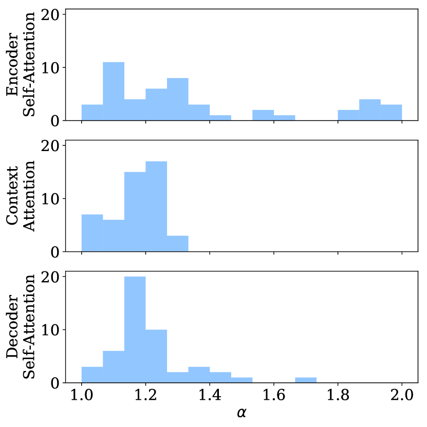
Figure 3: Distribution of learned $\alpha$ values per attention block. While the encoder self-attention has a bimodal distribution of values of $\alpha$, the decoder self-attention and context attention have a single mode.

Attention weight density when translating.

For any $\alpha>1$, it would still be possible for the weight matrices in Equation 3 to learn re-scalings so as to make attention sparser or denser. To visualize the impact of adaptive $\alpha$ values, we compare the empirical attention weight density (the average number of tokens receiving non-zero attention) within each module, against sparse Transformers with fixed $\alpha=1.5$.

Figure 4 shows that, with fixed $\alpha=1.5$, heads tend to be sparse and similarly-distributed in all three attention modules. With learned $\alpha$, there are two notable changes: (i) a prominent mode corresponding to fully dense probabilities, showing that our models learn to combine sparse and dense attention, and (ii) a distinction between the encoder self-attention – whose background distribution tends toward extreme sparsity – and the other two modules, who exhibit more uniform background distributions. This suggests that perhaps entirely sparse Transformers are suboptimal.

The fact that the decoder seems to prefer denser attention distributions might be attributed to it being auto-regressive, only having access to past tokens and not the full sentence. We speculate that it might lose too much information if it assigned weights of zero to too many tokens in the self-attention, since there are fewer tokens to attend to in the first place.

Teasing this down into separate layers, Figure 5 shows the average (sorted) density of each head for each layer. We observe that $\alpha$-entmax is able to learn different sparsity patterns at each layer, leading to more variance in individual head behavior, to clearly-identified dense and sparse heads, and overall to different tendencies compared to the fixed case of $\alpha=1.5$.

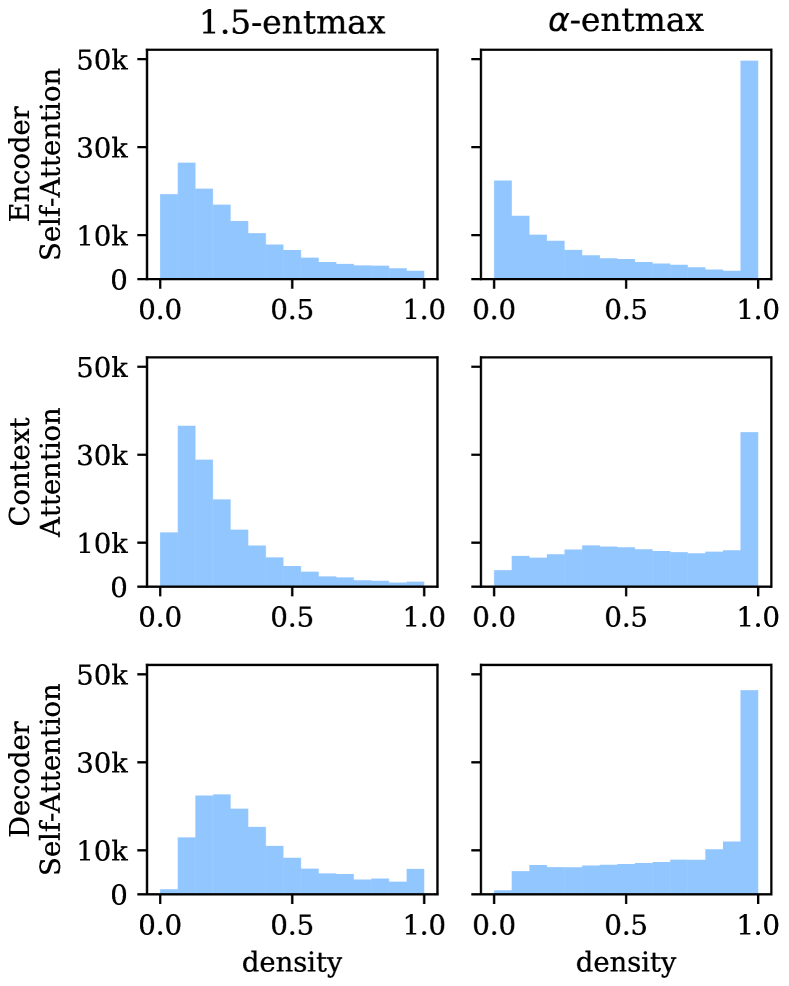
Figure 4: Distribution of attention densities (average number of tokens receiving non-zero attention weight) for all attention heads and all validation sentences. When compared to 1.5-entmax, $\alpha$-entmax distributes the sparsity in a more uniform manner, with a clear mode at fully dense attentions, corresponding to the heads with low $\alpha$. In the softmax case, this distribution would lead to a single bar with density 1.

Figure 5: Head density per layer for fixed and learned $\alpha$. Each line corresponds to an attention head; lower values mean that that attention head is sparser. Learned $\alpha$ has higher variance.

Head diversity.

To measure the overall disagreement between attention heads, as a measure of head diversity, we use the following generalization of the Jensen-Shannon divergence:

$$JS=\mathsf{H}^{\textsc{S}}\left(\frac{1}{H}\sum_{j=1}^{H}\bm{p}_{j}\right)-\frac{1}{H}\sum_{j=1}^{H}\mathsf{H}^{\textsc{S}}(\bm{p}_{j})$$ (11)

where $\bm{p}_{j}$ is the vector of attention weights assigned by head $j$ to each word in the sequence, and $\mathsf{H}^{\textsc{S}}$ is the Shannon entropy, base-adjusted based on the dimension of $\bm{p}$ such that $JS\leq 1$. We average this measure over the entire validation set. The higher this metric is, the more the heads are taking different roles in the model.

Figure 6 shows that both sparse Transformer variants show more diversity than the traditional softmax one. Interestingly, diversity seems to peak in the middle layers of the encoder self-attention and context attention, while this is not the case for the decoder self-attention.

The statistics shown in this section can be found for the other language pairs in Appendix A.

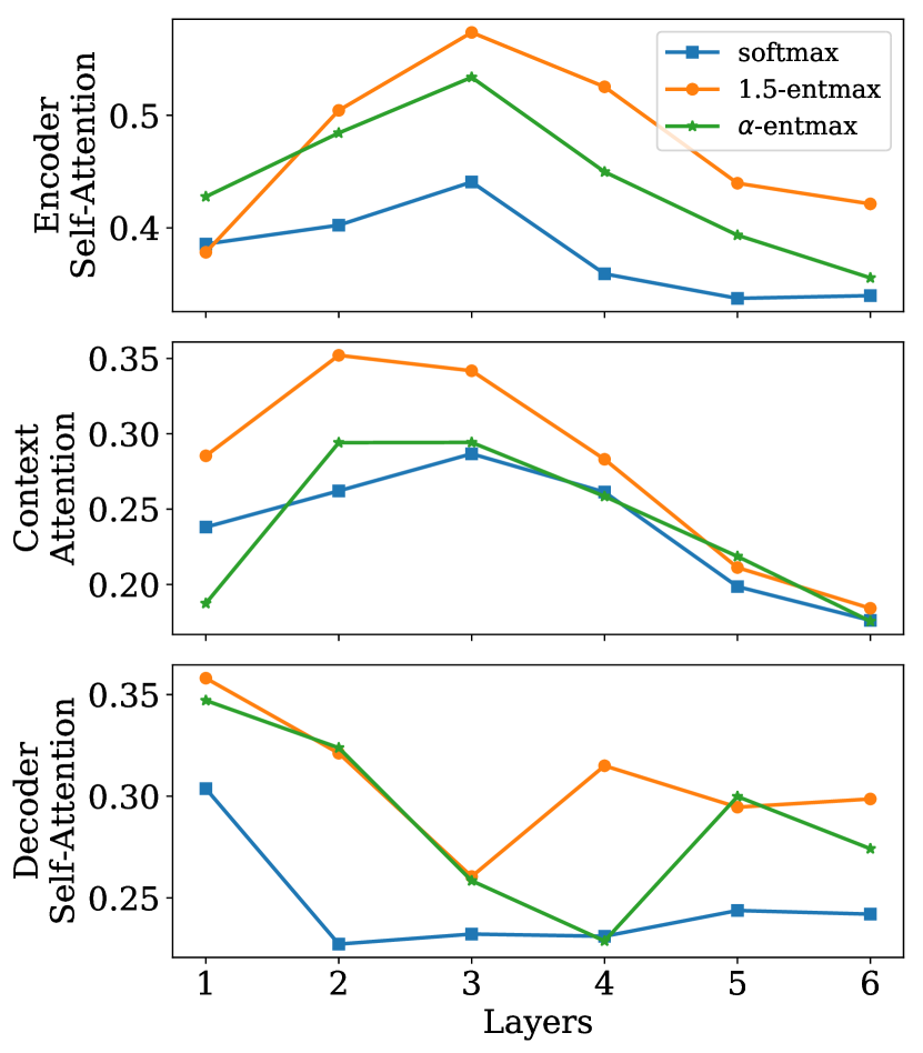
Figure 6: Jensen-Shannon Divergence between heads at each layer. Measures the disagreement between heads: the higher the value, the more the heads are disagreeing with each other in terms of where to attend. Models using sparse entmax have more diverse attention than the softmax baseline.

5.2 Identifying Head Specializations

Previous work pointed out some specific roles played by different heads in the softmax Transformer model (Voita et al., 2018; Tang et al., 2018; Voita et al., 2019). Identifying the specialization of a head can be done by observing the type of tokens or sequences that the head often assigns most of its attention weight; this is facilitated by sparsity.

Positional heads.

One particular type of head, as noted by Voita et al. (2019), is the positional head. These heads tend to focus their attention on either the previous or next token in the sequence, thus obtaining representations of the neighborhood of the current time step. In Figure 7, we show attention plots for such heads, found for each of the studied models. The sparsity of our models allows these heads to be more confident in their representations, by assigning the whole probability distribution to a single token in the sequence. Concretely, we may measure a positional head’s confidence as the average attention weight assigned to the previous token. The softmax model has three heads for position $-1$, with median confidence $93.5\%$. The $1.5$-entmax model also has three heads for this position, with median confidence $94.4\%$. The adaptive model has four heads, with median confidences $95.9\%$, the lowest-confidence head being dense with $\alpha=1.18$, while the highest-confidence head being sparse ($\alpha=1.91$).

For position $+1$, the models each dedicate one head, with confidence around $95\%$, slightly higher for entmax. The adaptive model sets $\alpha=1.96$ for this head.

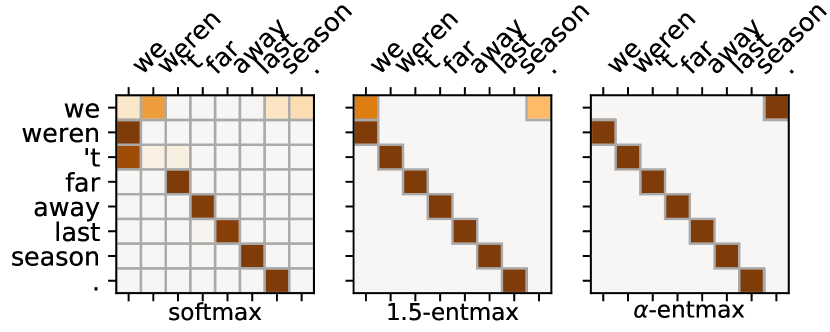
Figure 7: Self-attention from the most confidently previous-position head in each model. The learned parameter in the $\alpha$-entmax model is $\alpha=1.91$. Quantitatively more confident, visual inspection confirms that the adaptive head behaves more consistently.

BPE-merging head.

Due to the sparsity of our models, we are able to identify other head specializations, easily identifying which heads should be further analysed. In Figure 8 we show one such head where the $\alpha$ value is particularly high (in the encoder, layer 1, head 4 depicted in Figure 2). We found that this head most often looks at the current time step with high confidence, making it a positional head with offset $0$. However, this head often spreads weight sparsely over 2-3 neighboring tokens, when the tokens are part of the same BPE cluster or hyphenated words. As this head is in the first layer, it provides a useful service to the higher layers by combining information evenly within some BPE clusters.

For each BPE cluster or cluster of hyphenated words, we computed a score between 0 and 1 that corresponds to the maximum attention mass assigned by any token to the rest of the tokens inside the cluster in order to quantify the BPE-merging capabilities of these heads. There are not any attention heads in the softmax model that are able to obtain a score over $80\%$, while for $1.5$-entmax and $\alpha$-entmax there are two heads in each ($83.3\%$ and $85.6\%$ for $1.5$-entmax and $88.5\%$ and $89.8\%$ for $\alpha$-entmax).

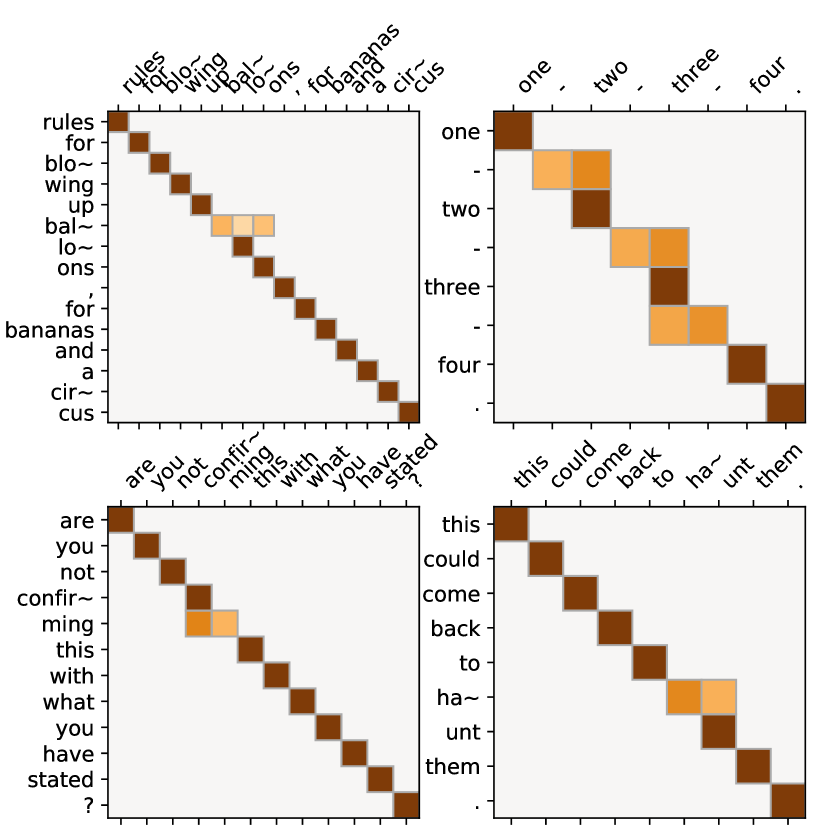
Figure 8: BPE-merging head $(\alpha=1.91)$ discovered in the $\alpha$-entmax model. Found in the first encoder layer, this head learns to discover some subword units and combine their information, leaving most words intact. It places $99.09\%$ of its probability mass within the same BPE cluster as the current token: more than any head in any other model.

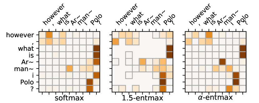
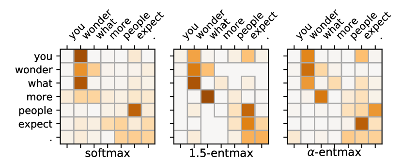
Figure 9: Interrogation-detecting heads in the three models. The top sentence is interrogative while the bottom one is declarative but includes the interrogative word “what”. In the top example, these interrogation heads assign a high probability to the question mark in the time step of the interrogative word (with $\geq 97.0\%$ probability), while in the bottom example since there is no question mark, the same head does not assign a high probability to the last token in the sentence during the interrogative word time step. Surprisingly, this head prefers a low $\alpha=1.05$, as can be seen from the dense weights. This allows the head to identify the noun phrase “Armani Polo” better.

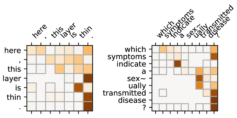
Figure 10: Example of two sentences of similar length where the same head ($\alpha=1.33$) exhibits different sparsity. The longer phrase in the example on the right “a sexually transmitted disease” is handled with higher confidence, leading to more sparsity.

Interrogation head.

On the other hand, in Figure 9 we show a head for which our adaptively sparse model chose an $\alpha$ close to 1, making it closer to softmax (also shown in encoder, layer 1, head 3 depicted in Figure 2). We observe that this head assigns a high probability to question marks at the end of the sentence in time steps where the current token is interrogative, thus making it an interrogation-detecting head. We also observe this type of heads in the other models, which we also depict in Figure 9. The average attention weight placed on the question mark when the current token is an interrogative word is $98.5\%$ for softmax, $97.0\%$ for $1.5$-entmax, and $99.5\%$ for $\alpha$-entmax.

Furthermore, we can examine sentences where some tendentially sparse heads become less so, thus identifying sources of ambiguity where the head is less confident in its prediction. An example is shown in Figure 10 where sparsity in the same head differs for sentences of similar length.

6 Related Work

Sparse attention.

Prior work has developed sparse attention mechanisms, including applications to NMT (Martins and Astudillo, 2016; Malaviya et al., 2018; Niculae and Blondel, 2017; Shao et al., 2019; Maruf et al., 2019). Peters et al. (2019) introduced the entmax function this work builds upon. In their work, there is a single attention mechanism which is controlled by a fixed $\alpha$. In contrast, this is the first work to allow such attention mappings to dynamically adapt their curvature and sparsity, by automatically adjusting the continuous $\alpha$ parameter. We also provide the first results using sparse attention in a Transformer model.

Fixed sparsity patterns.

Recent research improves the scalability of Transformer-like networks through static, fixed sparsity patterns (Child et al., 2019; Wu et al., 2019). Our adaptively-sparse Transformer can dynamically select a sparsity pattern that finds relevant words regardless of their position (e. g., Figure 9). Moreover, the two strategies could be combined. In a concurrent line of research, Sukhbaatar et al. (2019) propose an adaptive attention span for Transformer language models. While their work has each head learn a different contiguous span of context tokens to attend to, our work finds different sparsity patterns in the same span. Interestingly, some of their findings mirror ours – we found that attention heads in the last layers tend to be denser on average when compared to the ones in the first layers, while their work has found that lower layers tend to have a shorter attention span compared to higher layers.

Transformer interpretability.

The original Transformer paper (Vaswani et al., 2017) shows attention visualizations, from which some speculation can be made of the roles the several attention heads have. Mareček and Rosa (2018) study the syntactic abilities of the Transformer self-attention, while Raganato and Tiedemann (2018) extract dependency relations from the attention weights. Tenney et al. (2019) find that the self-attentions in BERT (Devlin et al., 2019) follow a sequence of processes that resembles a classical NLP pipeline. Regarding redundancy of heads, Voita et al. (2019) develop a method that is able to prune heads of the multi-head attention module and make an empirical study of the role that each head has in self-attention (positional, syntactic and rare words). Li et al. (2018) also aim to reduce head redundancy by adding a regularization term to the loss that maximizes head disagreement and obtain improved results. While not considering Transformer attentions, Jain and Wallace (2019) show that traditional attention mechanisms do not necessarily improve interpretability since softmax attention is vulnerable to an adversarial attack leading to wildly different model predictions for the same attention weights. Sparse attention may mitigate these issues; however, our work focuses mostly on a more mechanical aspect of interpretation by analyzing head behavior, rather than on explanations for predictions.

7 Conclusion and Future Work

We contribute a novel strategy for adaptively sparse attention, and, in particular, for adaptively sparse Transformers. We present the first empirical analysis of Transformers with sparse attention mappings (i. e., entmax), showing potential in both translation accuracy as well as in model interpretability.

In particular, we analyzed how the attention heads in the proposed adaptively sparse Transformer can specialize more and with higher confidence. Our adaptivity strategy relies only on gradient-based optimization, side-stepping costly per-head hyper-parameter searches. Further speed-ups are possible by leveraging more parallelism in the bisection algorithm for computing $\alpha$-entmax.

Finally, some of the automatically-learned behaviors of our adaptively sparse Transformers – for instance, the near-deterministic positional heads or the subword joining head – may provide new ideas for designing static variations of the Transformer.

Supplementary Material

Appendix A High-Level Statistics Analysis of Other Language Pairs

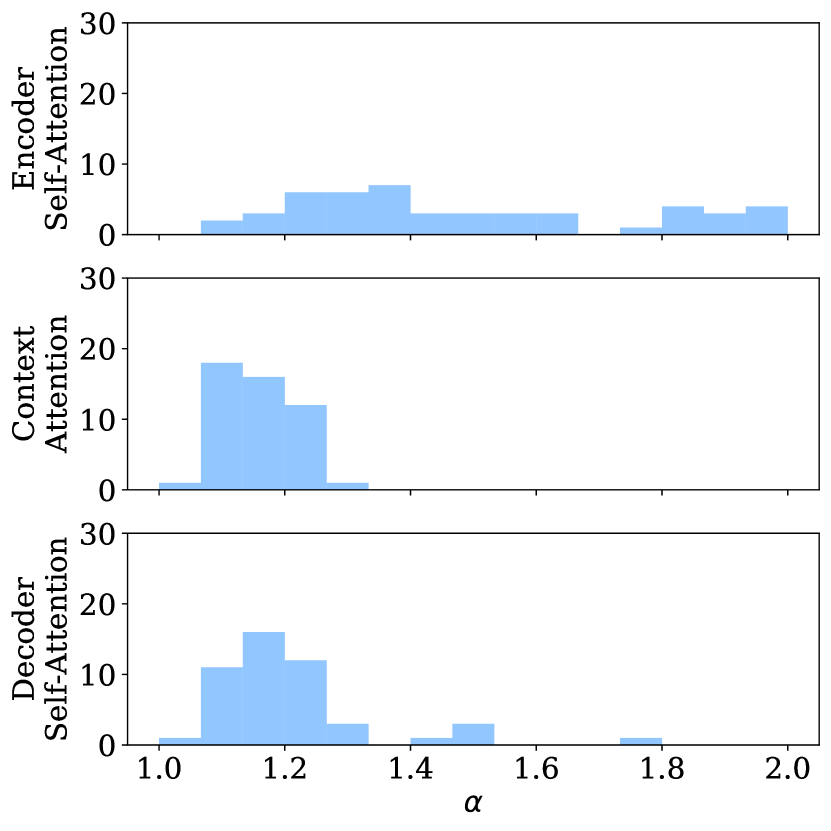
(a) WMT 2016 ro$\shortrightarrow$en.

(b) KFTT ja$\shortrightarrow$en.

(c) WMT 2014 en$\shortrightarrow$de.

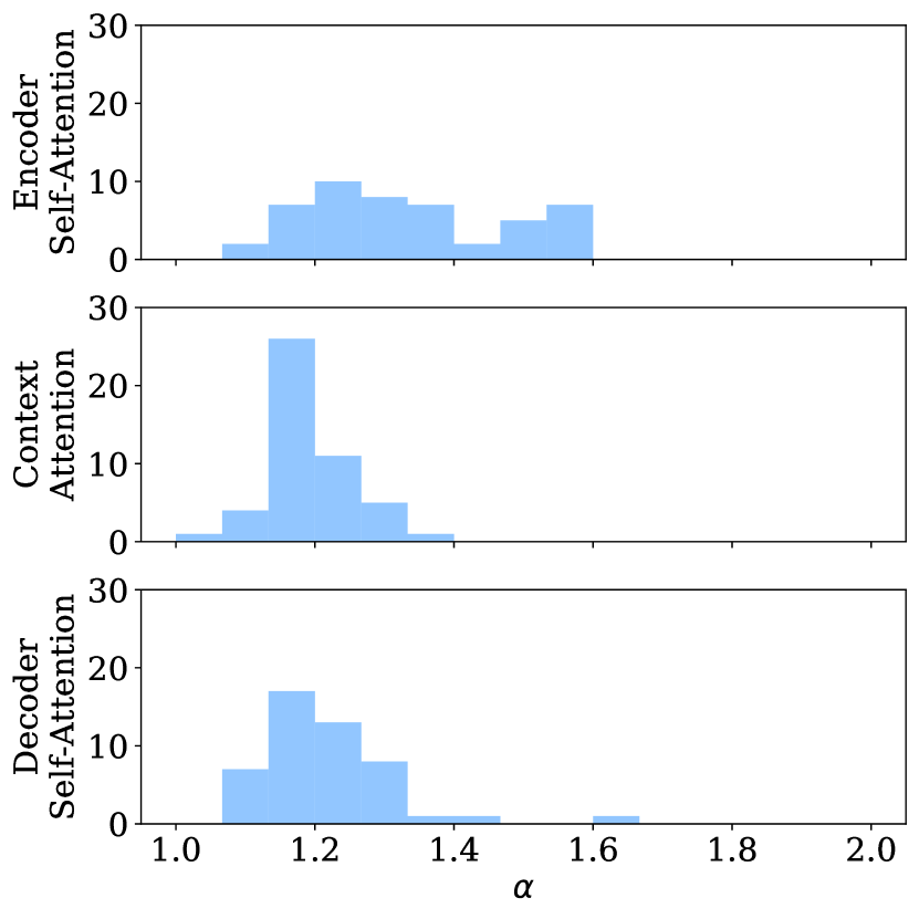
(d) IWSLT 2017 de$\shortrightarrow$en.

Figure 11: Histograms of $\alpha$ values.

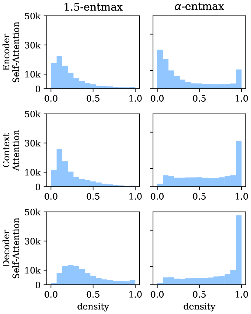
(a) WMT 2016 ro$\shortrightarrow$en.

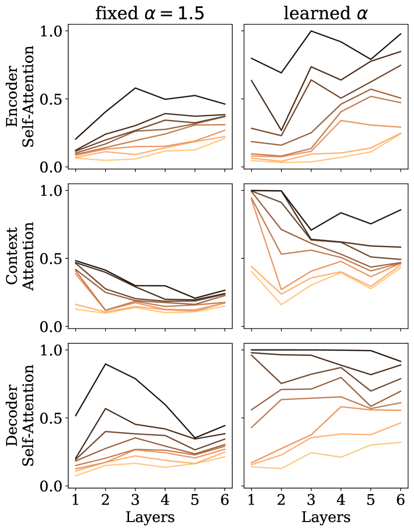
(b) KFTT ja$\shortrightarrow$en.

(c) WMT 2014 en$\shortrightarrow$de.

(d) IWSLT 2017 de$\shortrightarrow$en.

Figure 12: Histograms of head densities.

(a) WMT 2016 ro$\shortrightarrow$en.

(b) KFTT ja$\shortrightarrow$en.

(c) WMT 2014 en$\shortrightarrow$de.

(d) IWSLT 2017 de$\shortrightarrow$en.

Figure 13: Jensen-Shannon divergence over layers.

(a) WMT 2016 ro$\shortrightarrow$en.

(b) KFTT ja$\shortrightarrow$en.

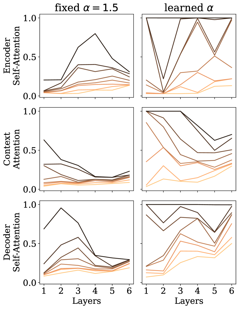
(c) WMT 2014 en$\shortrightarrow$de.

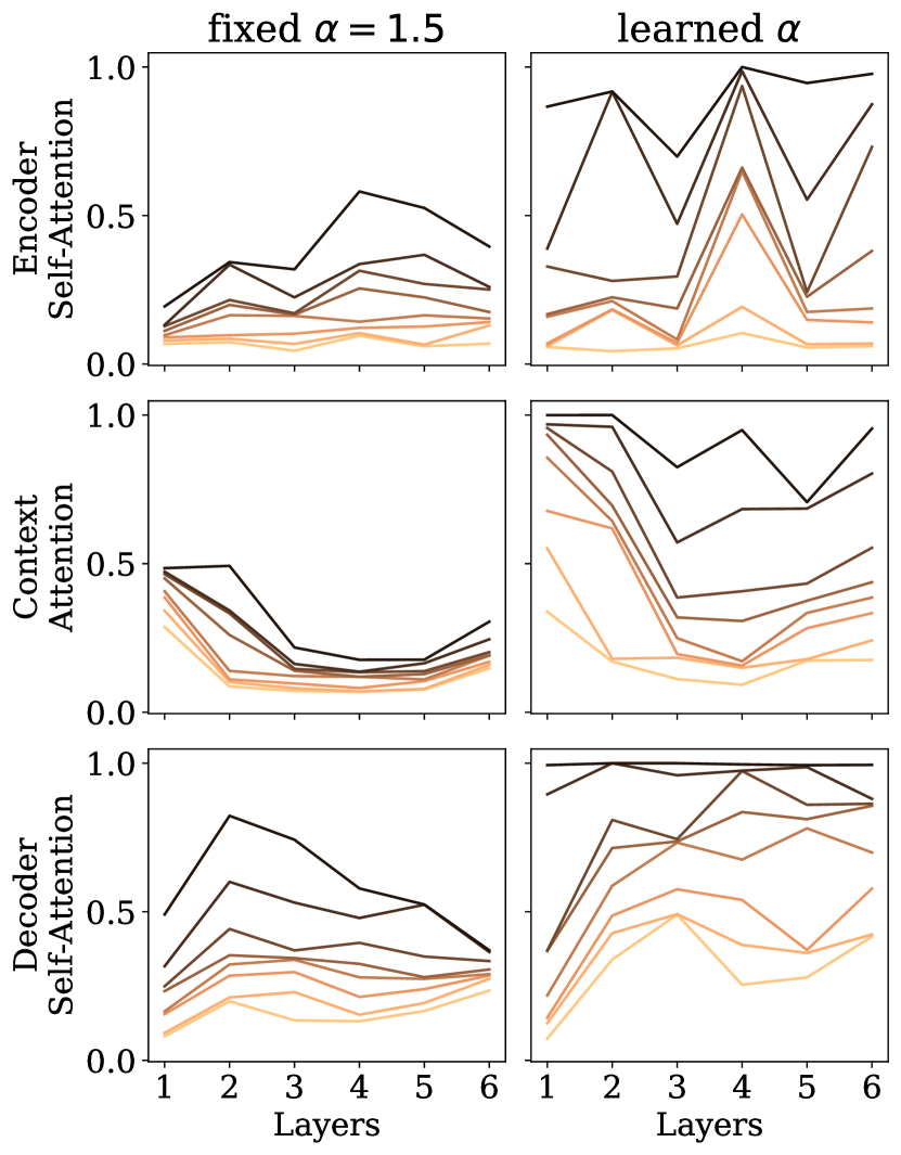
(d) IWSLT 2017 de$\shortrightarrow$en.

Figure 14: Head densities over layers.

Appendix B Background

B.1 Regularized Fenchel-Young prediction functions

Definition 1 (Blondel et al. 2019).

Let $\Omega\colon\triangle^{d}\to{\mathbb{R}}\cup\{\infty\}$ be a strictly convex regularization function. We define the prediction function $\bm{\pi}_{\Omega}$ as

$$\bm{\pi}_{\Omega}(\bm{z})=\operatorname*{\mathsf{argmax}}_{\bm{p}\in\triangle^{d}}\big{(}\bm{p}^{\top}\bm{z}-\Omega(\bm{p})\big{)}$$ (12)

B.2 Characterizing the $\alpha$-entmax mapping

Lemma 1 (Peters et al. 2019).

For any $\bm{z}$, there exists a unique $\tau^{\star}$ such that

$$\mathop{\mathsf{\alpha}\textnormal{-}\mathsf{entmax}}(\bm{z})=[(\alpha-1){\bm{z}}-\tau^{\star}\bm{1}]_{+}^{\nicefrac{{1}}{{\alpha-1}}}.$$ (13)

Proof: From the definition of $\mathop{\mathsf{\alpha}\textnormal{-}\mathsf{entmax}}$,

$$\mathop{\mathsf{\alpha}\textnormal{-}\mathsf{entmax}}(\bm{z})\coloneqq\operatorname*{\mathsf{argmax}}_{\bm{p}\in\triangle^{d}}\bm{p}^{\top}\bm{z}+\mathsf{H}^{\textsc{T}}_{\alpha}(\bm{p}),$$ (14)

we may easily identify it with a regularized prediction function (Def. 1):

$$\mathop{\mathsf{\alpha}\textnormal{-}\mathsf{entmax}}(\bm{z})\equiv\bm{\pi}_{-\mathsf{H}^{\textsc{T}}_{\alpha}}(\bm{z}).$$

We first note that for all $\bm{p}\in\triangle^{d}$,

$$-(\alpha-1)\mathsf{H}^{\textsc{T}}_{\alpha}(\bm{p})=\frac{1}{\alpha}\sum_{i=1}^{d}p_{i}^{\alpha}+\text{const}.$$ (15)

From the constant invariance and scaling properties of $\bm{\pi}_{\Omega}$ (Blondel et al., 2019, Proposition 1, items 4–5),

$$\bm{\pi}_{-\mathsf{H}^{\textsc{T}}_{\alpha}}(\bm{z})=\bm{\pi}_{\Omega}((\alpha-1)\bm{z}),\quad\text{with}\quad\Omega(\bm{p})=\sum_{j=1}^{d}g(p_{j}),\quad g(t)=\frac{t^{\alpha}}{\alpha}.$$

Using (Blondel et al., 2019, Proposition 5), noting that $g^{\prime}(t)=t^{\alpha-1}$ and $(g^{\prime})^{-1}(u)=u^{\nicefrac{{1}}{{\alpha-1}}}$, yields

$$\bm{\pi}_{\Omega}(\bm{z})=[\bm{z}-\tau^{\star}\bm{1}]_{+}^{\nicefrac{{1}}{{\alpha-1}}},\quad\text{and therefore}\quad\mathop{\mathsf{\alpha}\textnormal{-}\mathsf{entmax}}(\bm{z})=[(\alpha-1)\bm{z}-\tau^{\star}\bm{1}]_{+}^{\nicefrac{{1}}{{\alpha-1}}}.$$ (16)

Since $\mathsf{H}^{\textsc{T}}_{\alpha}$ is strictly convex on the simplex, $\mathop{\mathsf{\alpha}\textnormal{-}\mathsf{entmax}}$ has a unique solution $\bm{p}^{\star}$. Equation 16 implicitly defines a one-to-one mapping between $\bm{p}^{\star}$ and $\tau^{\star}$ as long as $\bm{p}^{\star}\in\triangle$, therefore $\tau^{\star}$ is also unique.   

B.3 Connections to softmax and sparsemax

The Euclidean projection onto the simplex, sometimes referred to, in the context of neural attention, as sparsemax (Martins and Astudillo, 2016), is defined as

$$\operatorname*{\mathsf{sparsemax}}(\bm{z})\coloneqq\operatorname*{\mathsf{argmin}}_{\bm{p}\in\triangle}\|\bm{p}-\bm{z}\|_{2}^{2}.$$ (17)

The solution can be characterized through the unique threshold $\tau$ such that $\sum_{i}\operatorname*{\mathsf{sparsemax}}(\bm{z})_{i}=1$ and (Held et al., 1974)

$$\operatorname*{\mathsf{sparsemax}}(\bm{z})=[\bm{z}-\tau\bm{1}]_{+}~{}.$$ (18)

Thus, each coordinate of the sparsemax solution is a piecewise-linear function. Visibly, this expression is recovered when setting $\alpha=2$ in the $\alpha$-entmax expression (Equation 21); for other values of $\alpha$, the exponent induces curvature.

On the other hand, the well-known softmax is usually defined through the expression

$$\operatorname*{\mathsf{softmax}}(\bm{z})_{i}\coloneqq\frac{\exp(z_{i})}{\sum_{j}\exp(z_{j})},$$ (19)

which can be shown to be the unique solution of the optimization problem

$$\operatorname*{\mathsf{softmax}}(\bm{z})_{i}=\operatorname*{\mathsf{argmax}}_{\bm{p}\in\triangle}\bm{p}^{\top}\bm{z}+\mathsf{H}^{\textsc{S}}(\bm{p}),$$ (20)

where $\mathsf{H}^{\textsc{S}}(\bm{p})\coloneqq-\sum_{i}p_{i}\log p_{i}$ is the Shannon entropy. Indeed, setting the gradient to $0$ yields the condition $\log p_{i}=z_{j}-\nu_{i}-\tau-1$, where $\tau$ and $\nu>0$ are Lagrange multipliers for the simplex constraints $\sum_{i}p_{i}=1$ and $p_{i}\geq 0$, respectively. Since the l. h .s. is only finite for $p_{i}>0$, we must have $\nu_{i}=0$ for all $i$, by complementary slackness. Thus, the solution must have the form $p_{i}=\nicefrac{{\exp(z_{i})}}{{Z}}$, yielding Equation 19.

Appendix C Jacobian of $\alpha$-entmax w. r .t. the shape parameter $\alpha$: Proof of Proposition 1

Recall that the entmax transformation is defined as:

$$\mathop{\mathsf{\alpha}\textnormal{-}\mathsf{entmax}}(\bm{z})\coloneqq\operatorname*{\mathsf{argmax}}_{\bm{p}\in\triangle^{d}}\bm{p}^{\top}\bm{z}+\mathsf{H}^{\textsc{T}}_{\alpha}(\bm{p}),$$ (21)

where $\alpha\geq 1$ and $\mathsf{H}^{\textsc{T}}_{\alpha}$ is the Tsallis entropy,

$$\mathsf{H}^{\textsc{T}}_{\alpha}(\bm{p})\!\coloneqq\!\begin{cases}\frac{1}{\alpha(\alpha-1)}\sum_{j}\!\left(p_{j}-p_{j}^{\alpha}\right)\!,&\!\!\!\alpha\neq 1,\\ \mathsf{H}^{\textsc{S}}(\bm{p}),&\!\!\!\alpha=1,\end{cases}$$ (22)

and $\mathsf{H}^{\textsc{S}}(\bm{p}):=-\sum_{j}p_{j}\log p_{j}$ is the Shannon entropy.

In this section, we derive the Jacobian of $\operatorname*{\mathsf{entmax}}$ with respect to the scalar parameter $\alpha$.

C.1 General case of $\alpha>1$

From the KKT conditions associated with the optimization problem in Eq. 21, we have that the solution $\bm{p}^{\star}$ has the following form, coordinate-wise:

$$p_{i}^{\star}=[(\alpha-1)(z_{i}-\tau^{\star})]_{+}^{1/(\alpha-1)},$$ (23)

where $\tau^{\star}$ is a scalar Lagrange multiplier that ensures that $\bm{p}^{\star}$ normalizes to 1, i. e., it is defined implicitly by the condition:

$$\sum_{i}[(\alpha-1)(z_{i}-\tau^{\star})]_{+}^{1/(\alpha-1)}=1.$$ (24)

For general values of $\alpha$, Eq. 24 lacks a closed form solution. This makes the computation of the Jacobian

$$\frac{\partial\mathop{\mathsf{\alpha}\textnormal{-}\mathsf{entmax}}(\bm{z})}{\partial\alpha}$$ (25)

non-trivial. Fortunately, we can use the technique of implicit differentiation to obtain this Jacobian.

The Jacobian exists almost everywhere, and the expressions we derive expressions yield a generalized Jacobian (Clarke, 1990) at any non-differentiable points that may occur for certain ($\alpha$, $\bm{z}$) pairs. We begin by noting that $\frac{\partial p_{i}^{\star}}{\partial\alpha}=0$ if $p_{i}^{\star}=0$, because increasing $\alpha$ keeps sparse coordinates sparse. Therefore we need to worry only about coordinates that are in the support of $\bm{p}^{\star}$. We will assume hereafter that the $i$^th coordinate of $\bm{p}^{\star}$ is non-zero. We have:

$$\frac{\partial p_{i}^{\star}}{\partial\alpha} = \frac{\partial}{\partial\alpha}[(\alpha-1)(z_{i}-\tau^{\star})]^{\frac{1}{\alpha-1}}$$ (26)

$$= \frac{\partial}{\partial\alpha}\exp\left[\frac{1}{\alpha-1}\log[(\alpha-1)(z_{i}-\tau^{\star})]\right]$$

$$= p_{i}^{\star}\frac{\partial}{\partial\alpha}\left[\frac{1}{\alpha-1}\log[(\alpha-1)(z_{i}-\tau^{\star})]\right]$$

$$= \frac{p_{i}^{\star}}{(\alpha-1)^{2}}\left[\frac{\frac{\partial}{\partial\alpha}[(\alpha-1)(z_{i}-\tau^{\star})]}{z_{i}-\tau^{\star}}-\log[(\alpha-1)(z_{i}-\tau^{\star})]\right]$$

$$= \frac{p_{i}^{\star}}{(\alpha-1)^{2}}\left[\frac{z_{i}-\tau^{\star}-(\alpha-1)\frac{\partial\tau^{\star}}{\partial\alpha}}{z_{i}-\tau^{\star}}-\log[(\alpha-1)(z_{i}-\tau^{\star})]\right]$$

$$= \frac{p_{i}^{\star}}{(\alpha-1)^{2}}\left[1-\frac{\alpha-1}{z_{i}-\tau^{\star}}\frac{\partial\tau^{\star}}{\partial\alpha}-\log[(\alpha-1)(z_{i}-\tau^{\star})]\right].$$

We can see that this Jacobian depends on $\frac{\partial\tau^{\star}}{\partial\alpha}$, which we now compute using implicit differentiation.

Let $\mathcal{S}=\{i:p^{\star}_{i}>0\}$). By differentiating both sides of Eq. 24, re-using some of the steps in Eq. 26, and recalling Eq. 23, we get

$$0 = \sum_{i\in\mathcal{S}}\frac{\partial}{\partial\alpha}[(\alpha-1)(z_{i}-\tau^{\star})]^{1/(\alpha-1)}$$ (27)

$$= \sum_{i\in\mathcal{S}}\frac{p_{i}^{\star}}{(\alpha-1)^{2}}\left[1-\frac{\alpha-1}{z_{i}-\tau^{\star}}\frac{\partial\tau^{\star}}{\partial\alpha}-\log[(\alpha-1)(z_{i}-\tau^{\star})]\right]$$

$$= \frac{1}{(\alpha-1)^{2}}-\frac{\partial\tau^{\star}}{\partial\alpha}\sum_{i\in\mathcal{S}}\frac{p_{i}^{\star}}{(\alpha-1)(z_{i}-\tau^{\star})}-\sum_{i\in\mathcal{S}}\frac{p_{i}^{\star}}{(\alpha-1)^{2}}\log[(\alpha-1)(z_{i}-\tau^{\star})]$$

$$= \frac{1}{(\alpha-1)^{2}}-\frac{\partial\tau^{\star}}{\partial\alpha}\sum_{i}(p_{i}^{\star})^{2-\alpha}-\sum_{i}\frac{p_{i}^{\star}}{\alpha-1}\log p_{i}^{\star}$$

$$= \frac{1}{(\alpha-1)^{2}}-\frac{\partial\tau^{\star}}{\partial\alpha}\sum_{i}(p_{i}^{\star})^{2-\alpha}+\frac{\mathsf{H}^{\textsc{S}}(\bm{p}^{*})}{\alpha-1},$$

from which we obtain:

$$\frac{\partial\tau^{\star}}{\partial\alpha} = \frac{\frac{1}{(\alpha-1)^{2}}+\frac{\mathsf{H}^{\textsc{S}}(\bm{p}^{\star})}{\alpha-1}}{\sum_{i}(p_{i}^{\star})^{2-\alpha}}.$$ (28)

Finally, plugging Eq. 28 into Eq. 26, we get:

$$\frac{\partial p_{i}^{\star}}{\partial\alpha} = \frac{p_{i}^{\star}}{(\alpha-1)^{2}}\left[1-\frac{1}{(p_{i}^{\star})^{\alpha-1}}\frac{\partial\tau^{\star}}{\partial\alpha}-(\alpha-1)\log p_{i}^{\star}\right]$$ (29)

$$= \frac{p_{i}^{\star}}{(\alpha-1)^{2}}\left[1-\frac{1}{(p_{i}^{\star})^{\alpha-1}}\frac{\frac{1}{(\alpha-1)^{2}}+\frac{\mathsf{H}^{\textsc{S}}(\bm{p}^{\star})}{\alpha-1}}{\sum_{i}(p_{i}^{\star})^{2-\alpha}}-(\alpha-1)\log p_{i}^{\star}\right]$$

$$= \frac{p_{i}^{\star}-\tilde{p}_{i}(\alpha)}{(\alpha-1)^{2}}-\frac{p_{i}^{\star}\log p_{i}^{\star}+\tilde{p}_{i}(\alpha)\mathsf{H}^{\textsc{S}}(\bm{p}^{\star})}{\alpha-1},$$

where we denote by

$$\tilde{p}_{i}(\alpha)=\frac{(p_{i}^{\star})^{2-\alpha}}{\sum_{j}(p_{j}^{\star})^{2-\alpha}}.$$ (30)

The distribution $\tilde{\bm{p}}(\alpha)$ can be interpreted as a “skewed” distribution obtained from $\bm{p}^{\star}$, which appears in the Jacobian of $\mathop{\mathsf{\alpha}\textnormal{-}\mathsf{entmax}}(\bm{z})$ w. r .t. $\bm{z}$ as well Peters et al. (2019).

C.2 Solving the indetermination for $\alpha=1$

We can write Eq. 29 as

$$\frac{\partial p_{i}^{\star}}{\partial\alpha} = \frac{p_{i}^{\star}-\tilde{p}_{i}(\alpha)-(\alpha-1)(p_{i}^{\star}\log p_{i}^{\star}+\tilde{p}_{i}(\alpha)\mathsf{H}^{\textsc{S}}(\bm{p}^{\star}))}{(\alpha-1)^{2}}.$$ (31)

When $\alpha\rightarrow 1^{+}$, we have $\tilde{\bm{p}}(\alpha)\rightarrow\bm{p}^{\star}$, which leads to a $\frac{0}{0}$ indetermination.

To solve this indetermination, we will need to apply L’Hôpital’s rule twice. Let us first compute the derivative of $\tilde{p}_{i}(\alpha)$ with respect to $\alpha$. We have

$$\frac{\partial}{\partial\alpha}(p_{i}^{\star})^{2-\alpha}=-(p_{i}^{\star})^{2-\alpha}\log p_{i}^{\star},$$ (32)

therefore

$$\frac{\partial}{\partial\alpha}\tilde{p}_{i}(\alpha) = \frac{\partial}{\partial\alpha}\frac{(p_{i}^{\star})^{2-\alpha}}{\sum_{j}(p_{j}^{\star})^{2-\alpha}}$$ (33)

$$= \frac{-(p_{i}^{\star})^{2-\alpha}\log p_{i}^{\star}\sum_{j}(p_{j}^{\star})^{2-\alpha}+(p_{i}^{\star})^{2-\alpha}\sum_{j}(p_{j}^{\star})^{2-\alpha}\log p_{j}^{\star}}{\left(\sum_{j}(p_{j}^{\star})^{2-\alpha}\right)^{2}}$$

$$= -\tilde{p}_{i}(\alpha)\log p_{i}^{\star}+\tilde{p}_{i}(\alpha)\sum_{j}\tilde{p}_{j}(\alpha)\log p_{j}^{\star}.$$

Differentiating the numerator and denominator in Eq. 31, we get:

$$\frac{\partial p_{i}^{\star}}{\partial\alpha} = \lim_{\alpha\rightarrow 1^{+}}\frac{(1+(\alpha-1)\mathsf{H}^{\textsc{S}}(\bm{p}^{\star}))\tilde{p}_{i}(\alpha)(\log p_{i}^{\star}-\sum_{j}\tilde{p}_{j}(\alpha)\log p_{j}^{\star})-p_{i}^{\star}\log p_{i}^{\star}-\tilde{p}_{i}(\alpha)\mathsf{H}^{\textsc{S}}(\bm{p}^{\star})}{2(\alpha-1)}$$ (34)

$$= A+B,$$

with

$$A = \lim_{\alpha\rightarrow 1^{+}}\frac{\mathsf{H}^{\textsc{S}}(\bm{p}^{\star})\tilde{p}_{i}(\alpha)(\log p_{i}^{\star}-\sum_{j}\tilde{p}_{j}(\alpha)\log p_{j}^{\star})\mathsf{H}^{\textsc{S}}(\bm{p}^{\star})}{2}$$ (35)

$$= \frac{\mathsf{H}^{\textsc{S}}(\bm{p}^{\star})p_{i}^{\star}\log p_{i}^{\star}+p_{i}^{\star}(\mathsf{H}^{\textsc{S}}(\bm{p}^{\star}))^{2}}{2},$$

and

$$B=\lim_{\alpha\rightarrow 1^{+}}\frac{\tilde{p}_{i}(\alpha)(\log p_{i}^{\star}-\sum_{j}\tilde{p}_{j}(\alpha)\log p_{j}^{\star})-p_{i}^{\star}\log p_{i}^{\star}-\tilde{p}_{i}(\alpha)\mathsf{H}^{\textsc{S}}(\bm{p}^{\star})}{2(\alpha-1)}.$$ (36)

When $\alpha\rightarrow 1^{+}$, $B$ becomes again a $\frac{0}{0}$ indetermination, which we can solve by applying again L’Hôpital’s rule. Differentiating the numerator and denominator in Eq. 36:

$$B = \frac{1}{2}\lim_{\alpha\rightarrow 1^{+}}\left\{\tilde{p}_{i}(\alpha)\log p_{i}^{\star}\left(\sum_{j}\tilde{p}_{j}(\alpha)\log p_{j}^{\star}-\log p_{i}^{\star}\right)\right.$$ (37)

$$-\tilde{p}_{i}(\alpha)\left(\sum_{j}\tilde{p}_{j}(\alpha)\log p_{j}^{\star}-\log p_{i}^{\star}\right)\left(\sum_{j}\tilde{p}_{j}(\alpha)\log p_{j}^{\star}+\mathsf{H}^{\textsc{S}}(\bm{p}^{\star})\right)$$

$$\left.-\tilde{p}_{i}(\alpha)\sum_{j}\tilde{p}_{j}(\alpha)\log p_{j}^{\star}\left(\sum_{k}\tilde{p}_{k}(\alpha)\log p_{k}^{\star}-\log p_{j}^{\star}\right)\right\}$$

$$= \frac{-p_{i}^{\star}\log p_{i}^{\star}(\mathsf{H}^{\textsc{S}}(\bm{p}^{\star})+\log p_{i}^{\star})+p_{i}^{\star}\sum_{j}p_{j}^{\star}\log p_{j}^{\star}(\mathsf{H}^{\textsc{S}}(\bm{p}^{\star})+\log p_{j}^{\star})}{2}$$

$$= \frac{-\mathsf{H}^{\textsc{S}}(\bm{p}^{\star})p_{i}^{\star}\log p_{i}^{\star}-p_{i}^{\star}(\mathsf{H}^{\textsc{S}}(\bm{p}^{\star}))^{2}-p_{i}^{\star}\log^{2}p_{i}^{\star}+p_{i}^{\star}\sum_{j}p_{j}^{\star}\log^{2}p_{j}^{\star}}{2}.$$

Finally, summing Eq. 35 and Eq. 37, we get

$$\frac{\partial p_{i}^{\star}}{\partial\alpha}\bigg{|}_{\alpha=1} = \frac{-p_{i}^{\star}\log^{2}p_{i}^{\star}+p_{i}^{\star}\sum_{j}p_{j}^{\star}\log^{2}p_{j}^{\star}}{2}.$$ (38)

C.3 Summary

To sum up, we have the following expression for the Jacobian of $\mathop{\mathsf{\alpha}\textnormal{-}\mathsf{entmax}}$ with respect to $\alpha$:

$$\frac{\partial p_{i}^{\star}}{\partial\alpha}=\left\{\begin{array}[]{ll}\frac{p_{i}^{\star}-\tilde{p}_{i}(\alpha)}{(\alpha-1)^{2}}-\frac{p_{i}^{\star}\log p_{i}^{\star}+\tilde{p}_{i}(\alpha)\mathsf{H}^{\textsc{S}}(\bm{p}^{\star})}{\alpha-1},&\text{for $\alpha>1$}\\ \frac{-p_{i}^{\star}\log^{2}p_{i}^{\star}+p_{i}^{\star}\sum_{j}p_{j}^{\star}\log^{2}p_{j}^{\star}}{2},&\text{for $\alpha=1$.}\end{array}\right.$$ (39)

References

- Amos and Kolter (2017) Brandon Amos and J. Zico Kolter. 2017. OptNet: Differentiable optimization as a layer in neural networks. In Proc. ICML.
- Bahdanau et al. (2015) Dzmitry Bahdanau, Kyunghyun Cho, and Yoshua Bengio. 2015. Neural machine translation by jointly learning to align and translate. In Proc. ICLR.
- Blondel et al. (2019) Mathieu Blondel, André FT Martins, and Vlad Niculae. 2019. Learning classifiers with Fenchel-Young losses: Generalized entropies, margins, and algorithms. In Proc. AISTATS.
- Bojar et al. (2014) Ondrej Bojar, Christian Buck, Christian Federmann, Barry Haddow, Philipp Koehn, Johannes Leveling, Christof Monz, Pavel Pecina, Matt Post, Herve Saint-Amand, et al. 2014. Findings of the 2014 workshop on statistical machine translation. In Proc. Workshop on Statistical Machine Translation.
- Bojar et al. (2016) Ondrej Bojar, Rajen Chatterjee, Christian Federmann, Yvette Graham, Barry Haddow, Matthias Huck, Antonio Jimeno Yepes, Philipp Koehn, Varvara Logacheva, Christof Monz, et al. 2016. Findings of the 2016 conference on machine translation. In Proc. WMT.
- Cettolo et al. (2017) M Cettolo, M Federico, L Bentivogli, J Niehues, S Stüker, K Sudoh, K Yoshino, and C Federmann. 2017. Overview of the IWSLT 2017 evaluation campaign. In Proc. IWSLT.
- Child et al. (2019) Rewon Child, Scott Gray, Alec Radford, and Ilya Sutskever. 2019. Generating long sequences with sparse Transformers. preprint arXiv:1904.10509.
- Clarke (1990) Frank H Clarke. 1990. Optimization and Nonsmooth Analysis. SIAM.
- Deng et al. (2018) Yuntian Deng, Yoon Kim, Justin Chiu, Demi Guo, and Alexander Rush. 2018. Latent alignment and variational attention. In Proc. NeurIPS.
- Devlin et al. (2019) Jacob Devlin, Ming-Wei Chang, Kenton Lee, and Kristina Toutanova. 2019. BERT: Pre-training of deep bidirectional transformers for language understanding. In Proc. NAACL-HLT.
- Gehring et al. (2017) Jonas Gehring, Michael Auli, David Grangier, Denis Yarats, and Yann N Dauphin. 2017. Convolutional sequence to sequence learning. In Proc. ICML.
- Gould et al. (2016) Stephen Gould, Basura Fernando, Anoop Cherian, Peter Anderson, Rodrigo Santa Cruz, and Edison Guo. 2016. On differentiating parameterized argmin and argmax problems with application to bi-level optimization. preprint arXiv:1607.05447.
- Held et al. (1974) Michael Held, Philip Wolfe, and Harlan P Crowder. 1974. Validation of subgradient optimization. Mathematical Programming, 6(1):62–88.
- Jain and Wallace (2019) Sarthak Jain and Byron C. Wallace. 2019. Attention is not explanation. In Proc. NAACL-HLT.
- Junczys-Dowmunt et al. (2018) Marcin Junczys-Dowmunt, Kenneth Heafield, Hieu Hoang, Roman Grundkiewicz, and Anthony Aue. 2018. Marian: Cost-effective high-quality neural machine translation in C++. In Proc. WNMT.
- Li et al. (2018) Jian Li, Zhaopeng Tu, Baosong Yang, Michael R Lyu, and Tong Zhang. 2018. Multi-Head Attention with Disagreement Regularization. In Proc. EMNLP.
- Louizos et al. (2018) Christos Louizos, Max Welling, and Diederik P Kingma. 2018. Learning sparse neural networks through regularization. Proc. ICLR.
- Luong et al. (2015) Minh-Thang Luong, Hieu Pham, and Christopher D Manning. 2015. Effective approaches to attention-based neural machine translation. In Proc. EMNLP.
- Malaviya et al. (2018) Chaitanya Malaviya, Pedro Ferreira, and André FT Martins. 2018. Sparse and constrained attention for neural machine translation. In Proc. ACL.
- Mareček and Rosa (2018) David Mareček and Rudolf Rosa. 2018. Extracting syntactic trees from Transformer encoder self-attentions. In Proc. BlackboxNLP.
- Martins and Astudillo (2016) André FT Martins and Ramón Fernandez Astudillo. 2016. From softmax to sparsemax: A sparse model of attention and multi-label classification. In Proc. of ICML.
- Maruf et al. (2019) Sameen Maruf, André FT Martins, and Gholamreza Haffari. 2019. Selective attention for context-aware neural machine translation. preprint arXiv:1903.08788.
- Neubig (2011) Graham Neubig. 2011. The Kyoto free translation task. http://www.phontron.com/kftt.
- Niculae and Blondel (2017) Vlad Niculae and Mathieu Blondel. 2017. A regularized framework for sparse and structured neural attention. In Proc. NeurIPS.
- Ott et al. (2018) Myle Ott, Sergey Edunov, David Grangier, and Michael Auli. 2018. Scaling neural machine translation. In Proc. WMT.
- Papineni et al. (2002) Kishore Papineni, Salim Roukos, Todd Ward, and Wei-Jing Zhu. 2002. BLEU: a method for automatic evaluation of machine translation. In Proc. ACL.
- Peters et al. (2019) Ben Peters, Vlad Niculae, and André FT Martins. 2019. Sparse sequence-to-sequence models. In Proc. ACL.
- Radford et al. (2019) Alec Radford, Jeffrey Wu, Rewon Child, David Luan, Dario Amodei, and Ilya Sutskever. 2019. Language models are unsupervised multitask learners. preprint.
- Raganato and Tiedemann (2018) Alessandro Raganato and Jörg Tiedemann. 2018. An analysis of encoder representations in Transformer-based machine translation. In Proc. BlackboxNLP.
- Sennrich et al. (2016) Rico Sennrich, Barry Haddow, and Alexandra Birch. 2016. Neural machine translation of rare words with subword units. In Proc. ACL.
- Shao et al. (2019) Wenqi Shao, Tianjian Meng, Jingyu Li, Ruimao Zhang, Yudian Li, Xiaogang Wang, and Ping Luo. 2019. SSN: Learning sparse switchable normalization via SparsestMax. In Proc. CVPR.
- Sukhbaatar et al. (2019) Sainbayar Sukhbaatar, Edouard Grave, Piotr Bojanowski, and Armand Joulin. 2019. Adaptive Attention Span in Transformers. In Proc. ACL.
- Tang et al. (2018) Gongbo Tang, Mathias Müller, Annette Rios, and Rico Sennrich. 2018. Why self-attention? A targeted evaluation of neural machine translation architectures. In Proc. EMNLP.
- Tenney et al. (2019) Ian Tenney, Dipanjan Das, and Ellie Pavlick. 2019. BERT rediscovers the classical NLP pipeline. In Proc. ACL.
- Tsallis (1988) Constantino Tsallis. 1988. Possible generalization of Boltzmann-Gibbs statistics. Journal of Statistical Physics, 52:479–487.
- Vaswani et al. (2017) Ashish Vaswani, Noam Shazeer, Niki Parmar, Jakob Uszkoreit, Llion Jones, Aidan N Gomez, Łukasz Kaiser, and Illia Polosukhin. 2017. Attention is all you need. In Proc. NeurIPS.
- Voita et al. (2018) Elena Voita, Pavel Serdyukov, Rico Sennrich, and Ivan Titov. 2018. Context-aware neural machine translation learns anaphora resolution. In Proc. ACL.
- Voita et al. (2019) Elena Voita, David Talbot, Fedor Moiseev, Rico Sennrich, and Ivan Titov. 2019. Analyzing multi-head self-attention: Specialized heads do the heavy lifting, the rest can be pruned. In Proc. ACL.
- Wu et al. (2019) Felix Wu, Angela Fan, Alexei Baevski, Yann N Dauphin, and Michael Auli. 2019. Pay less attention with lightweight and dynamic convolutions. In Proc. ICLR.