Low-$Q^{2}$ empirical parametrizations of the $N^{\ast}$ helicity amplitudes

Abstract

The data associated with the electromagnetic excitations of the nucleon ($\gamma^{\ast}N\to N^{\ast}$) are usually parametrized by helicity amplitudes at the resonance $N^{\ast}$ rest frame. The properties of the $\gamma^{\ast}N\to N^{\ast}$ transition current at low $Q^{2}$ can be, however, better understood when expressed in terms of structure form factors, particularly near the pseudothreshold, when the magnitude of the photon three-momentum vanishes ($|{\bf q}|=0$). At the pseudothreshold the invariant four-momentum square became $q^{2}=(M_{R}-M_{N})^{2}$, well in the timelike region $Q^{2}=-q^{2}<0$ [$M_{N}$ and $M_{R}$ are the mass of the nucleon and of the resonance, respectively]. In the helicity amplitude representation, the amplitudes have well-defined dependences on $|{\bf q}|$, near the pseudothreshold, and there are correlations between different amplitudes. Those constraints are often ignored in the empirical parametrizations of the helicity amplitudes. In the present work, we show that the structure of the transition current near the pseudothreshold has an impact on the parametrizations of the data. We present a method which modifies analytic parametrizations of the data at low $Q^{2}$, in order to take into account the constraints of the transition amplitudes near the pseudothreshold. The model dependence of the parametrizations on the low-$Q^{2}$ data is studied in detail.

I Introduction

In the past two decades, there was significant experimental progress in the study of the electromagnetic structure of the nucleon ($N$) and the nucleon excited states ($N^{\ast}$) NSTAR ; Aznauryan12b ; Puckett17 ; Drechsel2007 . From the theoretical point of view there was some progress in the description of the electromagnetic excitations $N^{\ast}$ using QCD sum rules Lenz09 ; Wang09 ; Anikin15 , approaches based on the Dyson-Schwinger equations Eichmann16 ; Segovia16 , AdS/QCD Teramond12 ; Brodsky15 ; Bayona12 ; Ramalho17 ; Gutsche and different classes of quark models Obukhovsky ; AznauryanII ; Santopinto ; NstarP1 ; SQTM . At low $Q^{2}$, the dynamical coupled-channel models which take into account the meson cloud dressing of the baryons are also successful Kamalov99 ; Drechsel2007 ; Burkert04 ; JDiaz07 .

The electromagnetic structure of the nucleon excitations can be probed through the scattering of electrons on nucleons ($eN\to e^{\prime}N^{\ast}$). The measured cross sections include the information about the $\gamma^{\ast}N\to N^{\ast}$ transitions, which can be expressed in terms of different structure functions depending on the photon polarization and on the four-momentum transfer squared, $q^{2}$. The most common representation of those structure functions is the helicity amplitude representation, where all the $\gamma^{\ast}N\to N^{\ast}$ transitions are parametrized in terms of the three different polarizations of the photon, including two transverse amplitudes $A_{1/2}$ and $A_{3/2}$ and one longitudinal amplitude $S_{1/2}$, depending on the angular momentum $J$ of the nucleon resonance $N^{\ast}$. Those amplitudes are usually presented in the rest frame of the resonance ($N^{\ast}$) Aznauryan12b ; Bjorken66 ; Jones73 ; Devenish76 ; Drechsel2007 .

An alternative representation of those structure functions is the transition form factor representation, generally derived from the structure of the $\gamma^{\ast}N\to N^{\ast}$ transition current Aznauryan12b ; Bjorken66 ; Jones73 ; Devenish76 ; Compton . Examples of the form factor representation are the Dirac and Pauli form factors, the electric and magnetic (Sachs) form factors of the nucleon Puckett17 . The nucleon resonances can also be described by the Dirac- and Pauli-like form factors for the $J=\frac{1}{2}^{\pm}$ resonances or multipole form factors, such as the electric, magnetic and Coulomb form factors for the $J=\frac{3}{2}^{\pm}$ resonances, with positive or negative parity ($P=\pm$) Jones73 ; Devenish76 ; Bjorken66 ; Compton ; Siegert1 ; Siegert2 . The form factor representation has some advantages in the interpretation of the structure of the $J^{\pm}$ states, since it emphasizes the symmetries associated with the nucleon resonances Compton .

Empirical parametrizations of the helicity amplitudes or transition form factors are important to compare with theoretical models and for calculations which require accurate descriptions of the $N^{\ast}$ data, in different ranges of $Q^{2}$ Compton ; Blin19a .

In general, the $J^{\pm}$ helicity amplitudes or the transition form factors are independent functions of $Q^{2}=-q^{2}$, except in some particular kinematic limits. An important limit is the pseudothreshold limit, where the magnitude of photon three-momentum $|{\bf q}|$ vanishes, and the nucleon and the nucleon resonance are both at rest. In this limit, the invariant $Q^{2}$ has the value $Q^{2}=-(M_{R}-M_{N})^{2}$, where $M_{N}$ and $M_{R}$ are the mass of the nucleon and the nucleon resonance $N^{\ast}$, respectively. Throughout this work, we also use $R$ to label $N^{\ast}$ and the properties of $N^{\ast}$.

The transition current associated with states $J=\frac{1}{2},\frac{3}{2}$ can be decomposed into two $\left(J=\frac{1}{2}\right)$ or three $\left(J=\frac{3}{2}\right)$ gauge-invariant terms associated with the properties of the transition. Each of those terms defines elementary form factors $G_{i}$ independent of each other and free of kinematical singularities Jones73 ; Devenish76 ; Bjorken66 . Helicity amplitudes in a given frame and the transition form factors (Dirac-Pauli or multipole) can be expressed as linear combinations of the elementary form factors $G_{i}$ Aznauryan12b ; Devenish76 ; Bjorken66 . The helicity amplitudes and transition form factors are not uncorrelated as the elementary form factors, because of the kinematical factors included in the transformation between the elementary form factors and the alternative structure functions. The discussion of those transformations and their consequences in the pseudothreshold limit can be found in Refs. Jones73 ; Devenish76 ; Bjorken66 .

When we parametrize the data in term of the elementary form factors $G_{i}$, we do not need to worry about the constraints at the pseudothreshold, since those are automatically ensured and the structure functions are free of kinematical singularities Devenish76 . Consistent parametrizations of the helicity amplitudes based on appropriated elementary form factors for the $J=\frac{1}{2},\frac{3}{2}$ resonances are presented in Ref. Compton .

When we parametrize the transition form factors or the helicity amplitudes at the resonance rest frame directly, however, we need to take into account the pseudothreshold constraints. Those structure functions are constrained by some specific dependence on $|{\bf q}|$ Drechsel92 ; AmaldiBook ; Tiator16 and by correlations between different helicity amplitudes and, equivalently, by correlations between transition form factors Jones73 ; Devenish76 ; Bjorken66 . Those constraints are the consequence of the gauge-invariant structure of the transition current and the kinematics associated with the $N^{\ast}$ rest frame Devenish76 ; Bjorken66 .

The dependence of the transverse amplitudes ($A_{1/2}$ and $A_{3/2}$) and longitudinal amplitudes in the magnitude of the photon three-momentum $|{\bf q}|$ for the cases $J=\frac{1}{2}^{\pm}$, $\frac{3}{2}^{\pm}$ is summarized in Table 1. Additional discussion about those relations can be found in Refs. Bjorken66 ; Devenish76 ; Jones73 ; Siegert1 ; Siegert2 ; Compton ; Drechsel92 . The content of the table shows that the constraints on the helicity amplitudes cannot be ignored if the pseudothreshold of the $\gamma^{\ast}N\to N^{\ast}$ transition is close to the photon point $Q^{2}=0$. This observation demonstrates the need of taking into account the pseudothreshold constraints in the empirical parametrizations of the helicity amplitudes, particularly for resonances with masses close to the nucleon.

$\frac{1}{2}^{+}$	$A_{1/2}\propto|{\bf q}|$,	$S_{1/2}\propto|{\bf q}|^{2}$
$\frac{1}{2}^{-}$	$A_{1/2}\propto 1$,	$S_{1/2}\propto|{\bf q}|$	$S_{1/2}\propto A_{1/2}|{\bf q}|$
$\frac{3}{2}^{+}$	$A_{1/2}\propto|{\bf q}|$,	$S_{1/2}\propto|{\bf q}|^{2}$	$S_{1/2}\propto(A_{1/2}-{\textstyle\frac{1}{\sqrt{3}}}A_{3/2})|{\bf q}|$
	$A_{3/2}\propto|{\bf q}|$,
$\frac{3}{2}^{-}$	$A_{1/2}\propto 1$,	$S_{1/2}\propto|{\bf q}|$	$S_{1/2}\propto(A_{1/2}+\sqrt{3}A_{3/2})|{\bf q}|$
	$A_{3/2}\propto 1$,		$(A_{1/2}-{\textstyle\frac{1}{\sqrt{3}}}A_{3/2})\propto|{\bf q}|^{2}$

Table 1: Constraints at the pseudothreshold.

The present work is motivated by the necessity of taking into account the constraints from Table 1 in the empirical parametrization of the data. Since the empirical parametrizations of the data ignore, in general, the specific dependence on $|{\bf q}|$, in the present work we checked if it is possible to modify those parametrizations below a certain value of $Q^{2}$, labeled as $Q_{P}^{2}$, in order to obtain a consistent extension to the pseudothreshold, without spoiling the description of the available data. We derive then analytic extensions of generic parametrizations of the data based on the continuity of the amplitudes and on the continuity of the first derivatives of those amplitudes in the transition point $Q_{P}^{2}$. With this procedure, we generate smooth extensions of available parametrizations of the data, and study the consistence of the results with the data and with the pseudothreshold constraints. The solutions obtained can also be used to test the sensibility of the solutions to possible variations of the data at low $Q^{2}$. This study is particularly useful, since there is generally a gap in the data between $Q^{2}=0$ and $Q^{2}=0.3$ GeV².

The formalism proposed to extend analytically the amplitudes to the timelike region is general and can be applied to any set of parametrizations of amplitudes, provided that those are continuous and that their first derivatives are also continuous in the spacelike region ($Q^{2}\geq 0$). To exemplify our formalism, we consider a particular set of empirical parametrizations of the $\gamma^{\ast}N\to N^{\ast}$ helicity amplitudes, associated with the $N^{\ast}$ states: $N(1440)$, $N(1520)$, $N(1535)$, $N(1650)$, $N(1710)$, $N(1720)$, $\Delta(1232)$, $\Delta(1620)$ and $\Delta(1700)$. We look, in particular, to the Jefferson Lab parametrizations from Ref. Jlab-fits , which have been used by several authors. Those parametrizations are based on simple expressions (rational functions of $\sqrt{Q^{2}}$), are, in general, valid in the range $Q^{2}=0.5$–5 GeV², and provide a fair description of the available data MokeevDatabase , in particular of the CLAS/JLab data CLAS09 ; CLAS12 ; Mokeev16 ; Blin19a at intermediate and large $Q^{2}$.

This article is organized as follows: In the next section, we discuss in more detail the implications of the pseudothreshold conditions on the helicity amplitudes. In Sec. III, we review the definition of the helicity amplitudes in the $N^{\ast}$ rest frame, and discuss which information is necessary to derive an analytic continuation of a given amplitude. The method used to extend the empirical parametrization to the timelike region, including the pseudothreshold limit, is presented in Sec. IV. The numerical results for all $N^{\ast}$ states considered are presented and analyzed in Sec. V. In Sec. VI we present our outlook and conclusions.

II Constraints on the Helicity amplitudes

The most popular consequence of the pseudothreshold constraints is the relation between the electric amplitude $E$ (combination of longitudinal amplitudes) and the scalar amplitude $S_{1/2}$ which can, in general, be expressed in the form

$$\lambda_{R}\,S_{1/2}=E\,|{\bf q}|,$$ (1)

where the factor $\lambda_{R}\propto(M_{R}-M_{N})$ depends on the masses of the nucleon and the resonance. The relation (1) is known as Siegert’s theorem or the long-wavelength theorem, since it is valid in the limit $|{\bf q}|\to 0$ Drechsel92 ; Buchmann98 ; Tiator16 . There are, however, other constraints, associated with the specific dependence of the amplitudes on $|{\bf q}|$, displayed in Table 1.

One can illustrate the importance of including the correct $|{\bf q}|$ dependence on the amplitudes, looking for the simplest case, the $\frac{1}{2}^{+}$ helicity amplitudes. Those amplitudes can be written as Aznauryan12b ; Roper

$$A_{1/2}={\cal R}\frac{|{\bf q}|}{\sqrt{1+\tau}}(\tau G_{1}+G_{2})$$

$$S_{1/2}=\frac{1}{\sqrt{2}(M_{R}+M_{N})}{\cal R}\frac{|{\bf q}|^{2}}{\sqrt{1+\tau}}(G_{1}-G_{2}),$$ (2)

where ${\cal R}$ is a constant, $\tau=\frac{Q^{2}}{(M_{R}+M_{N})^{2}}$, $\tau G_{1}$ represents the Dirac form factor and $G_{2}$ represents the Pauli form factor. Based on the previous representation, we conclude that if $G_{1}$ and $G_{2}$ are regular functions, with no zeros and singularities at the pseudothreshold, one has automatically $A_{1/2}\propto|{\bf q}|$ and $S_{1/2}\propto|{\bf q}|^{2}$. Most of the empirical parametrizations of the data based on parametrizations of the amplitudes $A_{1/2}$ and $S_{1/2}$ by regular functions, ignore this specific dependence on $|{\bf q}|$.

One concludes, then, that if the form factors ($G_{1}$ and $G_{2}$) are not parametrized directly, we need to enforce the dependence of the amplitudes on $|{\bf q}|$, in order to have a consistent parametrization of the data, based on the properties of the transition currents. Empirical parametrizations of the data which ignore the correct $|{\bf q}|$ dependence are inconsistent and provide erroneous descriptions of the helicity amplitudes at low $Q^{2}$.

There are in the literature several works which explore the relations between helicity amplitudes and transition form factors and try to identify in the data, signatures of the pseudothreshold constraints. The $\gamma^{\ast}N\to\Delta(1232)$ have been discussed in some detail by several authors Buchmann97a ; Buchmann98 ; Buchmann04 ; Tiator16 ; Drechsel2007 ; Siegert1 ; Siegert2 ; DeltaQuad ; RSM-Siegert ; GlobalP . The $\gamma^{\ast}N\to N(1535)$ and $\gamma^{\ast}N\to N(1520)$ are also discussed in Refs. Tiator16 ; Siegert1 ; Siegert2 . As for the states $\frac{1}{2}^{+}$, as the Roper, one can conclude from Table. 1, that there is no relation associated with Siegert’s theorem. This happens because for the $\frac{1}{2}^{+}$ states there is no electric amplitude Drechsel92 ; Drechsel2007 . Nevertheless, there are constraints for the amplitudes $A_{1/2}$ and $S_{1/2}$, which cannot be ignored.

Instead of deriving alternative parametrizations of the helicity amplitudes consistent with the pseudothreshold constraints, in the present work, we propose a method to modify available parametrizations of the data in order to satisfy those constraints. The consistence of the modified parametrizations with the low-$Q^{2}$ data can be checked afterwards.

III Empirical parametrizations of Helicity amplitudes

The experimental data associated with the $\gamma^{\ast}N\to N^{\ast}$ transitions are usually represented in term of the helicity amplitudes in the $N^{\ast}$ rest frame. Those amplitudes can be calculated from the transition current $J^{\mu}$, in units of the elementary charge $e$, using Aznauryan12b :

$$A_{3/2} = \sqrt{\frac{2\pi\alpha}{K}}\left<R,S_{z}^{\prime}=+{\textstyle\frac{3}{2}}\right|\epsilon_{+}\cdot J\left|N,S_{z}=+{\textstyle\frac{1}{2}}\right>$$

$$A_{1/2} = \sqrt{\frac{2\pi\alpha}{K}}\left<R,S_{z}^{\prime}=+{\textstyle\frac{1}{2}}\right|\epsilon_{+}\cdot J\left|N,S_{z}=-{\textstyle\frac{1}{2}}\right>$$

$$S_{1/2} = \sqrt{\frac{2\pi\alpha}{K}}\left<R,S_{z}^{\prime}=+{\textstyle\frac{1}{2}}\right|\epsilon_{0}\cdot J\left|N,S_{z}=+{\textstyle\frac{1}{2}}\right>\frac{|{\bf q}|}{Q},$$

where $S_{z}^{\prime}$ ($S_{z}$) is the final (initial) spin projection, ${\bf q}$ is the photon three-momentum in the rest frame of $R$, $Q=\sqrt{Q^{2}}$ and $\epsilon_{\lambda}^{\mu}$ ($\lambda=0,\pm 1$) are the photon polarization vectors. In the previous equations $\alpha\simeq 1/137$ is the fine-structure constant and $K=\frac{M_{R}^{2}-M_{N}^{2}}{2M_{R}}$ is the magnitude of the photon momentum when $Q^{2}=0$. In the rest frame of $R$ the magnitude of the nucleon three-momentum is $|{\bf q}|$, and reads

$$|{\bf q}|=\frac{\sqrt{Q_{+}^{2}Q_{-}^{2}}}{2M_{R}},$$ (6)

where $Q_{\pm}^{2}=(M_{R}\pm M_{N})^{2}+Q^{2}$.

Depending on the spin $J$ of the resonance one can have two ($J=\frac{1}{2}$) or three ($J=\frac{3}{2}$) independent amplitudes. There are in the literature several kinds of parametrizations of the data. The MAID (Mainz Unitary Isobar Model) parametrizations are characterized by the combination of polynomials and exponentials Drechsel2007 ; Siegert1 ; Siegert2 , and other parametrizations are based on rational functions Compton ; Aznauryan12b ; Siegert2 . In principle, all those parametrizations are equivalent in a certain range of $Q^{2}$, provided that $Q^{2}\geq 0$ and that we are not too close to the pseudothreshold.

The important for the following discussion is that the parametrization of a generic amplitude $A$ corresponds to a regular function of $Q^{2}$ (no zeros at $Q^{2}=0$ and no singularities), that the function is continuous and that the first derivatives exist and are also continuous.

We assume then that the parametrizations under discussion take known analytic forms, and describe well the data above a given threshold $Q_{P}^{2}>0$. In those cases we can check if we can derive analytic continuations to the timelike region consistent with the pseudothreshold constraints and with smooth transitions between the pseudothreshold $Q^{2}=-(M_{R}-M_{N})^{2}$ and the point $Q^{2}=Q_{P}^{2}$.

By varying the value of $Q_{P}^{2}$, we infer the sensibility of the fits to the pseudothreshold conditions. Since the empirical parametrizations of the data can be in some cases very sensitive to the low-$Q^{2}$ data, and also because there is in most resonances a gap between $Q^{2}=0$ and $Q^{2}=0.3$ GeV², we consider three different values for $Q_{P}^{2}$: $Q_{P}^{2}=0.1$ 0.3 and 0.5 GeV². We avoid intentionally the use of the $Q^{2}=0$, in order to derive an analytic continuation independent of the $Q^{2}=0$ data.

The analytic continuation is derived demanding a smooth transition between the region where the original parametrization is assumed to be valid, the $Q^{2}\geq Q_{P}^{2}$ region, and the region between the pseudothreshold, $Q^{2}=-(M_{R}-M_{N})^{2}$, and the point $Q^{2}=Q_{P}^{2}$. Below $Q^{2}=Q_{P}^{2}$ the parametrizations are consistent with the expected shape near the pseudothreshold, characterized by the expressions from Table 1. The smooth transition between the two regions is obtained by imposing the following conditions:

• The amplitude $A$ is continuous at $Q^{2}=Q_{P}^{2}$;

• the first derivative is continuous at $Q^{2}=Q_{P}^{2}$; and

• the second derivative is continuous at $Q^{2}=Q_{P}^{2}$.

In some cases, we demand also the continuity of the third derivative at $Q^{2}=Q_{P}^{2}$.

To derive the analytic continuation, we consider the expansion

$$A(Q^{2}) = A^{(0)}+A^{(1)}(Q^{2}-Q_{P}^{2})+$$

$$\frac{A^{(2)}}{2!}(Q^{2}-Q_{P}^{2})^{2}+\frac{A^{(3)}}{3!}(Q^{2}-Q_{P}^{2})^{3}+....,$$

where the coefficients $A^{(k)}$ ($k=1,2,3$) represent the derivatives $A^{(k)}=\frac{d^{k}A}{dQ^{2k}}(Q_{P}^{2})$ and $A^{(0)}=A(Q_{P}^{2})$. In the following, we refer to $A^{(k)}$ as the moments of the expansion of $A$ in $Q^{2}$.

The analytic continuation for the $-(M_{R}-M_{N})^{2}<Q^{2}<Q_{P}^{2}$ region is discussed in the next section.

$\frac{1}{2}^{+}$	$A_{1/2}=a_{0}\tilde{q}+a_{1}\tilde{q}^{3}+a_{2}\tilde{q}^{5}+a_{3}\tilde{q}^{7}$		$S_{1/2}=c_{0}\tilde{q}^{2}+c_{1}\tilde{q}^{4}+c_{2}\tilde{q}^{6}+c_{3}\tilde{q}^{8}$
$\frac{1}{2}^{-}$	$A_{1/2}=a_{0}+a_{1}\tilde{q}^{2}+a_{2}\tilde{q}^{4}+a_{3}\tilde{q}^{6}$		$S_{1/2}={\bf c_{0}}\tilde{q}+c_{1}\tilde{q}^{3}+c_{2}\tilde{q}^{5}+c_{3}\tilde{q}^{5}$
$\frac{3}{2}^{+}$	$A_{1/2}=a_{0}\tilde{q}+a_{1}\tilde{q}^{3}+a_{2}\tilde{q}^{5}+a_{3}\tilde{q}^{7}$	$A_{3/2}=b_{0}\tilde{q}+b_{1}\tilde{q}^{3}+b_{2}\tilde{q}^{5}+b_{3}\tilde{q}^{7}$	$S_{1/2}={\bf c_{0}}\tilde{q}^{2}+c_{1}\tilde{q}^{4}+c_{2}\tilde{q}^{6}+c_{3}\tilde{q}^{8}$
$\frac{3}{2}^{-}$	$A_{1/2}=a_{0}+a_{1}\tilde{q}^{2}+a_{2}\tilde{q}^{4}+a_{3}\tilde{q}^{6}$	$A_{3/2}={\bf b_{0}}+b_{1}\tilde{q}^{2}+b_{2}\tilde{q}^{4}+b_{3}\tilde{q}^{6}$	$S_{1/2}={\bf c_{0}}\tilde{q}+c_{1}\tilde{q}^{3}+c_{2}\tilde{q}^{5}+c_{3}\tilde{q}^{7}$

Table 2: Parametrizations of the helicity amplitudes for the cases $\frac{1}{2}^{\pm}$ and $\frac{3}{2}^{\pm}$.

IV Analytic extension of the helicity amplitudes to the timelike region

In the region $-(M_{R}-M_{N})^{2}<Q^{2}<Q_{P}^{2}$, we consider a formal representation of the helicity amplitudes in terms of the variable $|{\bf q}|$ defined by Eq. (6), in order to parametrize the leading-order dependence of the amplitudes near the pseudothreshold. The connection between $Q^{2}$ and $|{\bf q}|$ can be obtained by the inversion of the relation (6):

$$Q^{2}=-(M_{R}-M_{N})^{2}+2M_{R}\left[\sqrt{M_{N}^{2}+|{\bf q}|^{2}}-M_{N}\right].$$

(8)

More specifically, we represent the helicity amplitudes using an expansion in powers of $|{\bf q}|^{2}$ in the form

$$A=|{\bf q}|^{n}(\alpha_{0}+\alpha_{1}|{\bf q}|^{2}+\alpha_{2}|{\bf q}|^{4}+\alpha_{3}|{\bf q}|^{6}),$$ (9)

for the cases $n=0,1,2$. The representation (9) is consistent with all the amplitudes from Table 1. The coefficients $\alpha_{0}$, $\alpha_{1}$, $\alpha_{2}$ and $\alpha_{3}$ are determined by the connection with the $Q^{2}>Q_{P}^{2}$ region and the continuity conditions associated with the amplitudes, the first and the second derivatives of the amplitudes, as discussed next. In some cases we use also the continuity of the third derivative.

Note that in Eq. (9) there are no odd powers of $|{\bf q}|$ in the second factor. This representation is motivated by the relation between the derivative in $|{\bf q}|$ and $Q^{2}$, from where we can conclude that the odd terms vanish near the pseudothreshold.

Instead of the variable $|{\bf q}|^{2}$, one can use the dimensionless variable

$$\tilde{q}^{2}=\frac{|{\bf q}|^{2}}{M_{R}^{2}}.$$ (10)

For simplicity, we define also $\tilde{q}=\sqrt{\tilde{q}^{2}}$. Using the new notation, we can parametrize the amplitudes for the $\frac{1}{2}^{\pm}$ and $\frac{3}{2}^{\pm}$ resonances in the form

$$A=\tilde{q}^{n}(\alpha_{0}+\alpha_{1}\tilde{q}^{2}+\alpha_{2}\tilde{q}^{4}+\alpha_{3}\tilde{q}^{6}),$$ (11)

where all the coefficients $\alpha_{l}$ ($l=0,1,2,3$) have the same dimensions, the dimension of the helicity amplitudes (GeV^-1/2). The explicit parametrizations for the resonances under study are in Table 2.

In Table 2, we use $a_{l}$, $b_{l}$ and $c_{l}$ ($l=0,1,2,3$) to represent the coefficients of the amplitudes $A_{1/2}$, $A_{3/2}$ and $S_{1/2}$, respectively. The effect of the factor $\tilde{q}^{n}$ in Eq. (11) can be taken into account by redefining $A$ as $\frac{A}{\tilde{q}}$ or $\frac{A}{\tilde{q}^{2}}$.

The coefficients $\alpha_{l}$ ($l=0,1,2,3$) are determined based on the correlations between the amplitudes (pseudothreshold conditions) and the continuity conditions for $A$ and their derivatives, characterized by the moments $A^{(k)}$ ($k=0,1,2,3$). There are two cases to be considered:

1. The amplitude is independent of the pseudothreshold conditions.

2. The amplitude is correlated with another amplitude.

In the first case, we can determine all coefficients using the continuity of $A$ and the first three derivatives at the point $Q^{2}=Q_{P}^{2}$ to fix all the coefficients. The last coefficient $\alpha_{3}$ is in this case determined by $A^{(3)}$ (third derivative of $A$).

In the second case we use the correlation condition to fix the first coefficient ($\alpha_{0}$) and the remaining coefficients are determined by the continuity of the amplitude and the first two derivatives at the point $Q^{2}=Q_{P}^{2}$.

The explicit expressions for the two cases are presented in Appendix A for the function (11) for the case $n=0$. The other cases can be obtained using the corresponding results for $\frac{A}{\tilde{q}}$ or $\frac{A}{\tilde{q}^{2}}$. The relations between the coefficients $\alpha_{l}$ and the moments of the expansion in $Q^{2}$ from Eq. (LABEL:eqAmp1) are presented in Appendix B.

Since the longitudinal amplitude ($S_{1/2}$) is, in general, poorly constrained near $Q^{2}=0$, because there are no measurements at $Q^{2}=0$, in our calculations we choose to fix the coefficients of $S_{1/2}$ using the correlations with the transverse amplitudes.

The coefficients of the transverse amplitudes ($A_{1/2}$ and $A_{3/2}$) can, in principle, be considered independent of the pseudothreshold conditions. In those conditions all the coefficients can be determined using the continuity of the amplitude and the first three derivatives, as mentioned above. The states $\frac{3}{2}^{-}$ are the exception to this role because the two transverse amplitudes are also correlated, as shown in the second column in Table 1.

We now consider the different $J^{P}$ states.

IV.1 $\frac{1}{2}^{+}$ states

For the $\frac{1}{2}^{+}$ states there are no special constraints at the pseudothreshold, except for the forms

$$A_{1/2}\propto|{\bf q}|,\hskip 17.07182ptS_{1/2}\propto|{\bf q}|^{2},$$ (12)

presented in Table 1.

In the present case, we can determine all coefficients of the amplitudes $A_{1/2}$ and $S_{1/2}$ demanding the continuity of the amplitudes and the first three derivatives independently, since those amplitudes are uncorrelated (case 1).

From the parametrizations from Ref. Jlab-fits , there are two resonances to be taken into account: $N(1440)$ (Roper) and $N(1710)$.

IV.2 $\frac{1}{2}^{-}$ states

The $\frac{1}{2}^{-}$ states are characterized by the relation Devenish76 ; Siegert1

$$A_{1/2}=\sqrt{2}(M_{R}-M_{N})\frac{S_{1/2}}{|{\bf q}|}.$$ (13)

The previous relation is equivalent to Eq. (1), since $E\propto A_{1/2}$.

An alternative view of the pseudothreshold constraints is obtained when we consider the Dirac ($F_{1}$) and Pauli ($F_{2}$) form factors. In that case we can write, near the pseudothreshold $A_{1/2}=2b\tilde{F}_{1}$ and $S_{1/2}=\sqrt{2}b\frac{|{\bf q}|}{M_{R}-M_{N}}\tilde{F}_{1}$, where $\tilde{F}_{1}=F_{1}+\frac{M_{R}-M_{N}}{M_{R}+M_{N}}F_{2}$ and $b\propto\sqrt{Q_{+}^{2}}$ is a known function Siegert1 . Check Ref. Siegert1 for more details.

According to the parametrizations from Table 2, the condition (13) corresponds to

$$\sqrt{2}\frac{M_{R}-M_{N}}{M_{R}}c_{0}=a_{0}.$$ (14)

The bold variable $\mathbf{c_{0}}$ in Table 2 indicates that $c_{0}$ is fixed by (14).

The amplitude $A_{1/2}$ can be considered independent with the coefficients determined by the continuity conditions of the amplitude and the first three derivatives (case 1). The coefficient $c_{0}$ is determined by the value of $a_{0}$. The remaining coefficients $c_{l}$ ($l=1,2,3$) are determined by the continuity conditions associated with the amplitude $S_{1/2}$ and the first two derivatives (case 2).

This formalism can be used for the states $N(1535)$, $N(1650)$ and $\Delta(1620)$.

IV.3 $\frac{3}{2}^{+}$ states

The ${\textstyle\frac{3}{2}}^{+}$ are constrained by the condition between electric and Coulomb Jones-Scadron form factors Devenish76 ; Jones73

$$G_{E}=\frac{M_{R}-M_{N}}{2M_{R}}G_{C}.$$ (15)

When expressed in terms of helicity amplitudes, we obtain the relations $G_{E}=F_{+}\left(A_{1/2}-{\textstyle\frac{1}{\sqrt{3}}}A_{3/2}\right)$ and $\frac{|{\bf q}|}{2M_{R}}G_{C}=F_{+}\sqrt{2}S_{1/2}$, where $F_{+}\propto 1/|{\bf q}|$ is a kinematic factor. One obtains then the relation between amplitudes Jones73

$$A_{1/2}-\frac{1}{\sqrt{3}}A_{3/2}=\sqrt{2}\frac{M_{R}-M_{N}}{|{\bf q}|}S_{1/2}.$$ (16)

According to the parametrizations from Table 2, the previous equation is equivalent to

$$\sqrt{2}\frac{M_{R}-M_{N}}{M_{R}}c_{0}=a_{0}-\frac{b_{0}}{\sqrt{3}}.$$ (17)

An additional consequence of the relations $A_{1/2}\propto|{\bf q}|$ and $A_{3/2}\propto|{\bf q}|$ is that

$$G_{M}\propto(A_{1/2}-{\textstyle\frac{1}{\sqrt{3}}}A_{3/2})/|{\bf q}|\propto 1,$$ (18)

near the pseudothreshold, meaning that $G_{M}$ is finite when $|{\bf q}|\to 0$ Siegert2 ; Compton .

In the present case the amplitudes $A_{1/2}$ and $A_{3/2}$ are uncorrelated and all coefficients can be determined independently using the continuity of the amplitudes and the first three derivatives (case 1). The coefficient $c_{0}$ is determined afterwards using Eq. (17). The remaining coefficients are determined by the continuity of the function and the first two derivatives at the point $Q^{2}=Q_{P}^{2}$ (case 2).

This formalism can be applied to the resonances $\Delta(1232)$ and $N(1720)$.

IV.4 $\frac{3}{2}^{-}$ states

Contrary to the previous cases there are two conditions at the pseudothreshold: Siegert2 ; Compton ; Devenish76 ; Aznauryan12b :

$$G_{E}=-\frac{M_{R}-M_{N}}{M_{N}}G_{C},$$ (19)

$$G_{M}\propto|{\bf q}|^{2}.$$ (20)

One has then two constraints for the three form factors. When expressed in terms of the helicity amplitudes, we obtain:

$$A_{1/2}+\sqrt{3}A_{3/2}=-2\sqrt{2}\frac{M_{R}-M_{N}}{|{\bf q}|}S_{1/2},$$ (21)

$$A_{1/2}-\frac{1}{\sqrt{3}}A_{3/2}\propto|{\bf q}|^{2}.$$ (22)

Based on the parametrization from Table 2, we derive the relations between coefficients

$$b_{0}=\sqrt{3}a_{0},$$ (23)

$$-\frac{M_{R}-M_{N}}{\sqrt{2}M_{R}}c_{0}=a_{0}.$$ (24)

In the case of the resonances $\frac{3}{2}^{-}$ one has then two constraints for the three amplitudes expressed by Eqs. (23) and (24). Since $a_{0}$ appears in both conditions, we use the continuity of $A_{1/2}$ and the first three derivatives to fix the coefficients $a_{l}$ first (case 1). After that, we fix the coefficients $b_{0}$ and $c_{0}$ using Eqs. (23) and (24) and determine the remaining coefficients through the continuity of $A_{3/2}$ and $S_{1/2}$ and the first two derivatives (case 2).

The present formalism can be applied to the resonances $N(1520)$ and $\Delta(1700)$.

      

      

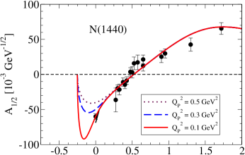
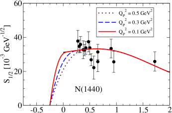
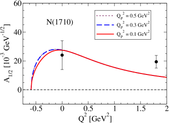
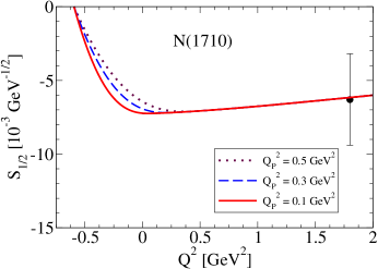
Figure 1: $\gamma^{\ast}N\to N^{\ast}\left(\frac{1}{2}^{+}\right)$ transition amplitudes. $N^{\ast}=N(1440)$, $N(1710)$. Data for $N(1440)$ from Refs. PDG14 ; CLAS09 ; CLAS12 ; Mokeev16 . The lowest point for $S_{1/2}$ are from MAMI Stajner17 . Data for $N(1710)$ from Refs PDG14 ; Park15 (three data points for $Q^{2}>2$ GeV² are not shown).

      

      

      

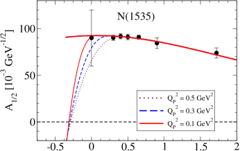
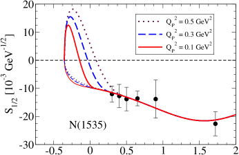
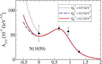
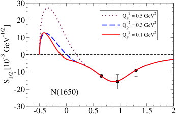
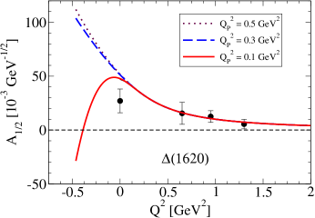
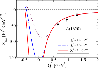
Figure 2: $\gamma^{\ast}N\to N^{\ast}\left(\frac{1}{2}^{-}\right)$ transition amplitudes. $N^{\ast}=N(1535)$, $N(1650)$, $\Delta(1620)$. The tick lines for the $N(1535)$ describe alternative parametrizations discussed in the main text. Data for $N(1535)$ from Ref. PDG14 ; CLAS09 . Data for $N(1650)$ from Ref. PDG14 ; Mokeev14 . Data for $\Delta(1620)$ from Ref. PDG14 ; Mokeev16 .

V Numerical results

We present now the numerical results associated with different $\frac{1}{2}^{\pm}$ and $\frac{3}{2}^{\pm}$ states.

The formalism discussed in the previous section is general, and can be applied to any regular set of parametrizations of the amplitudes, in the spacelike region (the amplitudes and the first derivatives are continuous).

To exemplify the method, we consider the empirical parametrizations from the Jefferson Lab from Ref. Jlab-fits . Those parametrizations are based on simple rational expressions, in general, are valid in the range $Q^{2}=0.5$–5 GeV², and provide a fair description of the available data, in particular the CLAS data.

To study the sensibility of the analytic extensions to the transition point between the original parametrization and our analytic extension ($Q_{P}^{2}$), we consider the values $Q_{P}^{2}=0.1$, 0.3 and 0.5 GeV².

Our analytic extensions are also compared directly with the data, particularly the database from Ref. MokeevDatabase . We recall that the $N^{\ast}$ helicity amplitude data are, in general, scarce, except for the states $\Delta(1232)\frac{3}{2}^{+}$, $N(1440)\frac{1}{2}^{+}$, $N(1520)\frac{3}{2}^{-}$ and $N(1535)\frac{1}{2}^{-}$. The data for most of the other states are incomplete, since they are restricted mainly to the transverse amplitudes and also restricted to three or five data points. For these reasons, we select, in particular, data from CLAS: The CLAS data are complete and cover a wide range in $Q^{2}$.

Another limitation of the data is that there is a lack of data in the region $Q^{2}=0$–0.3 GeV². As a consequence, the analytic extrapolations for the low-$Q^{2}$ region are very sensitive to the available data, leading to ambiguities in the extrapolations to the $Q^{2}<0$ region. These effects are sometimes amplified by the correlation between the amplitudes near the pseudothreshold.

Of particular importance is the experimental determination of the transverse amplitudes at the photon point ($Q^{2}=0$). Different groups provide very different estimates for those amplitudes. In some some cases, the Particle Data Group (PDG) summarizes the results using an interval with a large window of variation.

Our results for the resonances $\frac{1}{2}^{+}$, $\frac{1}{2}^{-}$, $\frac{3}{2}^{+}$ and $\frac{3}{2}^{-}$ are presented in Figs. 1, 2, 3 and 4, respectively. The tables with the coefficients associated to each parametrization are presented in Appendix C. In all cases, we include the original fit (solid dark line) in the $Q^{2}>0$ region, although the line is not always visible due to the overlap of lines.

The states $\Delta(1232)\frac{3}{2}^{+}$, $N(1440)\frac{1}{2}^{+}$, $N(1520)\frac{3}{2}^{-}$ and $N(1535)\frac{1}{2}^{-}$ are discussed first. Later, we analyze the remaining cases.

V.1 $N(1440)\frac{1}{2}^{+}$

Our results for $N(1440)\frac{1}{2}^{+}$ are at the top in Fig. 1.

The $N(1440)\frac{1}{2}^{+}$ state is interesting, because there is no direct relation between the two amplitudes. The effect of the pseudothreshold is restricted to the leading-order dependence of the amplitudes on $|{\bf q}|$ near the pseudothreshold, presented in Eqs. (12). Nevertheless, there are still interesting features in the different extension for the timelike region depending on the value of $Q^{2}_{P}$.

From the results for the amplitude $A_{1/2}$ we can conclude that the extrapolations for $Q^{2}<Q_{P}^{2}$ are very sensitive to the value of $Q_{P}^{2}$. This happens because the original parametrization has a large derivative near $Q^{2}=0$ in order to describe the $Q^{2}=0$ data. All the extrapolations attempt to provide a smooth transition between the result at $Q^{2}=0$ and the result at the pseudothreshold ($A_{1/2}=0$). Note, however, that the parametrization with $Q_{P}^{2}=0.1$ GeV² has a strong deflection near $Q^{2}=0$ inducing a significant increment of the magnitude of the amplitude followed by a fast reduction to zero at the pseudothreshold. The extension associated with $Q_{P}^{2}=0.3$ GeV² is the one with the best balance between the description of the data and a smoother transition to the pseudothreshold, and it is also close to the $Q^{2}=0$ data point. The $A_{1/2}$ amplitude provides a good example about the sensitivity of the parametrizations to the low-$Q^{2}$ data.

As for the amplitude $S_{1/2}$ all the parametrizations are consistent with the data, except for the lowest $Q^{2}$ point from MAMI (Mainz Microtron) ($Q^{2}=0.1$ GeV²) Stajner17 .

Only new data below $Q^{2}=0.3$ GeV² can help to determine the shape of $A_{1/2}$ and $S_{1/2}$ near $Q^{2}=0$, and to select which analytic extension is better.

       

       

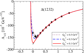
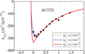
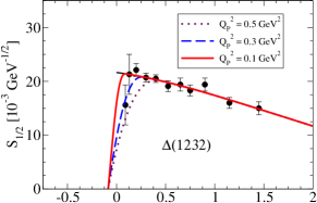
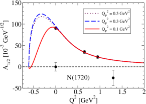
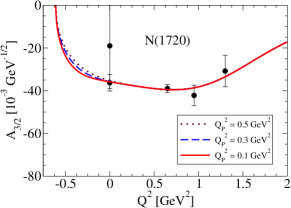
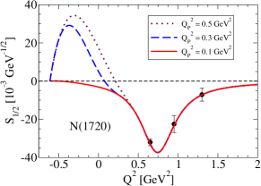
Figure 3: $\gamma^{\ast}N\to N^{\ast}\left(\frac{3}{2}^{+}\right)$ transition amplitudes. $N^{\ast}=$ $\Delta(1232)$, $N(1720)$. Data for $\Delta(1232)$ from Refs. PDG14 ; CLAS09 ; Stave08 ; Sparveris13 ; Blomberg16a . Data for $N(1720)$ from Refs. PDG14 ; Mokeev16b . For the $N(1720)$ we include also the result at $Q^{2}=0$ from Refs. Dugger09 used in the parametrization.

V.2 $N(1535)\frac{1}{2}^{-}$

Our results for the $N(1535)\frac{1}{2}^{-}$ are at the top in Fig. 2. We discuss first the results represented by the thick lines.

From the graphs for $A_{1/2}$ we can conclude that all the extensions are equivalent. The results for $S_{1/2}$, however, are very different. The strong dependence of the analytic extensions on the point $Q_{P}^{2}$ is clear from the graph. This result shows how relevant the pseudothreshold condition (13) is, since the extrapolation demands a positive derivative for $S_{1/2}$ near the pseudothreshold. It is worth mentioning that similar shapes can be obtained when we use phenomenological motivated parametrizations similar to the ones from MAID (combination of polynomials and exponentials) Siegert1 .

The exact point where the function $S_{1/2}$ starts to approach zero when $Q^{2}$ decreases, still in the spacelike region ($Q^{2}>0$), cannot be determined by the data, since there are no $S_{1/2}$ data below $Q^{2}=0.3$ GeV². Our extrapolation for the timelike region provides then an excellent example of how important measurements are below $Q^{2}=0.3$ GeV².

Our results for $N(1535)\frac{1}{2}^{-}$ provide another example of the impact of the pseudothreshold in the parametrizations of the data. Based on the available $S_{1/2}$ data, we cannot distinguish between the three analytic extensions for $Q^{2}<0$. Only future and accurate data can decide which extension for the $Q^{2}<0.5$ GeV² region is better.

In the present case it can be interesting to discuss the constraints imposed in the parametrizations of $A_{1/2}$ and $S_{1/2}$. We recall that we chose the situation where the parametrization of $A_{1/2}$ is fixed by the continuity of the amplitude and the first three derivatives of the amplitude at $Q^{2}=Q_{P}^{2}$, while for $S_{1/2}$ we demanded only the continuity of the amplitude and the first two derivatives. We impose then stronger conditions for $A_{1/2}$, since as mentioned the function $A_{1/2}$ is constrained more accurately by the data, since the error bars are smaller and we have an estimate of $A_{1/2}$ at $Q^{2}=0$. As a consequence of those constraints, all extensions of $A_{1/2}$ are described by smooth functions, almost undistinguished between them (overlap of thick lines). All those extensions are consistent with a very small third derivative of $A_{1/2}$ near $Q^{2}=0$.

From the graph for $A_{1/2}$, one can notice, however, that the data point at $Q^{2}=0$ has a very large errorbar. In the present case, this happens because the data selected by the PDG have a large dispersion, and the PDG considers a very large window of variation. Since $A_{1/2}(0)$ is poorly determined, one can question if the use of the amplitude $A_{1/2}$ as a reference is, in fact, a good choice and if we should not consider the hypothesis of using the amplitude $S_{1/2}$ as a reference, although based on data with larger errorbars. If we use this alternative procedure, we are replacing a parametrization derived from the condition that the third derivative of $A_{1/2}$ is small ($A_{1/2}^{(3)}\approx 0$), by a parametrization that assumes that it is the function $S_{1/2}$ that is smooth, with coefficients determined by the first three derivatives of $S_{1/2}$. In that case we used Eq. (13) to determine the shape of $A_{1/2}$ near the pseudothreshold based on the shape of $S_{1/2}$.

In order to test the impact of this alternative method to the pseudothreshold constraints, we recalculate the parameters of the amplitudes $A_{1/2}$ and $S_{1/2}$ based on the previous hypothesis: Fix $S_{1/2}$ by the first three derivatives and $A_{1/2}$ by Eq. (13) and the first two derivatives, also for the points $Q_{P}^{2}=0.1$, 0.3, and 0.5 GeV². The new estimates are represented in the graphs by the thin lines with the same convention. It is clear from the graphs that $A_{1/2}$ is not described by smooth functions near $Q^{2}=0$. The results for $A_{1/2}$ are now described by functions consistent with a large $A_{1/2}^{(3)}$.

As for the amplitude $S_{1/2}$, it is now described by very smooth functions of $Q^{2}$ in the timelike region. All the extensions of $S_{1/2}$ are now very similar.

We emphasize that both descriptions (thin lines and thick lines) are consistent with the available data, where one has a gap in the region $Q^{2}=0$–0.3 GeV², and the large error for $A_{1/2}(0)$. One concludes, then that only new data for $S_{1/2}$ or more accurate result for $A_{1/2}(0)$ can decide which description of the low-$Q^{2}$ data is the best.

V.3 $\Delta(1232)\frac{3}{2}^{+}$

Our results for the $\Delta(1232)\frac{3}{2}^{+}$ are at the top in Fig. 3.

From the graphs we can conclude that the parametrization characterized by $Q_{P}^{2}=0.3$ GeV² (dashed line) is the one that better describes the data, more specifically, the $Q^{2}<0.3$ GeV² data. There are two main explanations for this result. A possible explanation is the fact that the parametrizations from Ref. Jlab-fits are based on simple rational functions of $Q=\sqrt{Q^{2}}$ and, therefore, do not try to describe in detail the low-$Q^{2}$ region, since they are more focused on the $Q^{2}=0.5$–5 GeV² region. Another explanation is that the photon point ($Q^{2}=0$) is in the present case very close to the pseudothreshold $Q^{2}=-(M_{R}-M_{N})^{2}\simeq-0.09$ GeV². The consequence of the closeness between those two points is that the pseudothreshold constraints (17), and $A_{1/2},A_{3/2}\propto|{\bf q}|$ demand a sharp variation between the results near $Q^{2}=0$ and the pseudothreshold, where all the amplitudes vanish, although with different rates.

       

       

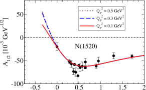
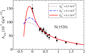
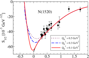
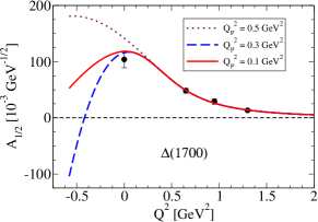
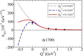
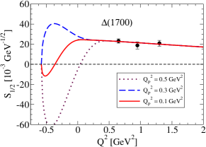
Figure 4: $\gamma^{\ast}N\to N^{\ast}\left(\frac{3}{2}^{-}\right)$ transition amplitudes. $N^{\ast}=$ $N(1520)$, $\Delta(1700)$. Data for $N(1520)$ from Refs. PDG14 ; CLAS09 ; CLAS12 ; Mokeev16 . Data for $\Delta(1700)$ from Refs. PDG14 ; Mokeev14 .

The sharp variation near the pseudothreshold can be understood in simple terms, noting that, using the dominance of the magnetic form factor ($G_{M}$) over the electric form factor ($G_{E}$), we can write Jones73 ; NDelta

$$A_{1/2}=-{\cal B}G_{M},\hskip 8.5359ptA_{3/2}=-\sqrt{3}{\cal B}G_{M},$$ (25)

where

$${\cal B}=\frac{1}{2}\frac{M_{R}}{M_{N}}\sqrt{\frac{\pi\alpha}{MM_{R}K}}\frac{|{\bf q}|}{\sqrt{1+\tau}}\propto|{\bf q}|.$$ (26)

In the region $-(M_{R}-M_{N})^{2}\leq Q^{2}\leq 0$ one can approximate $\sqrt{1+\tau}\simeq 1$ with an accuracy better than 1%. In these conditions $A_{1/2}$ and $A_{3/2}$ are determined exclusively by $G_{M}$.

Assuming that $G_{M}$ is a smooth function of $Q^{2}$ in the interval $[-(M_{R}-M_{N})^{2},0]$, we can write

$$G_{M}(Q^{2})\simeq G_{M}(0)+G_{M}^{\prime}(0)Q^{2}$$

$$\simeq[G_{M}(0)-G_{M}^{\prime}(0)(M_{R}-M_{N})^{2}]+G_{M}^{\prime}(0)\frac{M_{R}}{M_{N}}|{\bf q}|^{2},$$

where the use the expansion $Q^{2}\simeq-(M_{R}-M_{N})^{2}+\frac{M_{R}}{M_{N}}|{\bf q}|^{2}$, for small $|{\bf q}|$ based on Eq. (8).

A simple estimate with the MAID 2007 parametrization Drechsel2007 gives $G_{M}(Q^{2})\simeq 3.75-10.17\frac{|{\bf q}|^{2}}{M_{N}^{2}}$. Based on the previous result, one obtains

$$A_{1/2}\simeq\frac{A_{3/2}}{\sqrt{3}}=-b\left(3.75-10.17\frac{|{\bf q}|^{2}}{M_{N}^{2}}\right)|{\bf q}|,$$ (28)

where $b=0.0908$ GeV^-3/2. The leading-order term is then corrected by a term in $|{\bf q}|^{3}$ ensuring a smooth transition to the $Q^{2}>0$ region.

The study of the pseudothreshold constraints on the $\gamma^{\ast}N\to\Delta(1232)$ transition can also be performed using the form factor representation, based on Siegert’s theorem (15). From the theoretical point of view, the electric and Coulomb form factor data at low $Q^{2}$ can be described by a combination of valence quark and pion cloud effects LatticeD , where both contributions are compatible with the relation (15) DeltaQuad ; RSM-Siegert ; GlobalP .

The data presented in Fig. 3 deserve some discussion. Contrary to most of the resonances there are for the $\Delta(1232)$ finite $Q^{2}$ data below $Q^{2}=0.3$ GeV². The database from Ref. MokeevDatabase includes data from CLAS CLAS09 and low-$Q^{2}$ data from different sources such as MAMI Stave08 , MIT-Bates MIT_data ; Sparveris13 , and data at $Q^{2}=0$ from the PDG PDG14 . In the present study, however, we replaced the data for $Q^{2}<0.15$ GeV² by more recent estimates of the data. Concerning the data for $Q^{2}=0$ for $A_{1/2}$ and $A_{3/2}$, we use the data associated to $G_{M}(0)$ and the ratio $R_{EM}=-\frac{G_{E}(0)}{G_{M}(0)}$, also from the PDG PDG14 . This procedure is justified by the difference of results for the form factors obtained when we use the helicity amplitudes Pascalutsa07b .

As for the $Q^{2}<0.15$ GeV² data, we replace the results from MAMI and MIT-Bates ($Q^{2}=0.06$ and 0.127 GeV²) Stave08 ; MIT_data ; Sparveris13 by the recent results from JLab/Hall A ($Q^{2}=0.09$ and 0.13 GeV²) Blomberg16a . This procedure is motivated by the conclusion that there are errors in the previous analysis which lead to an overestimation of the results for $G_{E}$ and $G_{C}$, as discussed in Refs. Blomberg16a ; RSM-Siegert . The data for $A_{1/2}$, $A_{3/2}$ and $S_{1/2}$ presented here are converted from the results for the form factors presented in Refs. RSM-Siegert ; GlobalP . For the conversion, we used the MAID 2007 parametrization Drechsel2007 for the magnetic form factor, since it is simple and accurate in the region of study.

V.4 $N(1520)\frac{3}{2}^{-}$

Our results for the $N(1520)\frac{3}{2}^{-}$ are at the top in Fig. 4.

From the graphs we conclude that the amplitudes $A_{3/2}$ and $S_{1/2}$ are very sensitive to $Q_{P}^{2}$, while the amplitude $A_{1/2}$ is almost independent of $Q_{P}^{2}$ in the $Q^{2}>0$ region. From all the analytic extensions only the parametrizations with $Q_{P}^{2}=0.1$ GeV² are consistent with the data for $A_{3/2}(0)$. As for the amplitude $S_{1/2}$, all the extensions are valid, since there are no data for $Q^{2}<0.3$ GeV².

Overall, we can conclude that the parametrizations with $Q_{P}^{2}=0.1$ GeV² provide a smooth extrapolation to the timelike region and are consistent with the available data.

V.5 Other resonances

The remaining resonances show that some amplitudes are very sensitive to the threshold of the extrapolation (value of $Q_{P}^{2})$. This result is also a consequence of the limited data used in the calibrations (between three and five points) combined with the nonexistent data below $Q^{2}=0.5$ GeV², except for $Q^{2}=0$.

The exception is the state $N(1710)\frac{1}{2}^{+}$. Those results are a consequence of the lack of constraints, apart from the relations (12), and also to the more significant distance between the $Q^{2}=0$ data and the pseudothreshold. This distance is about $0.6$ GeV², much larger than the $N(1440)$ case ($\approx 0.25$ GeV²). In the case of the $N(1710)$, there is more room for the amplitudes to fall down to the pseudothreshold.

Concerning the resonance $\Delta(1620)\frac{1}{2}^{-}$, a note about the parametrizations from Ref. Jlab-fits is in order. The original parametrization has the form $S_{1/2}\propto 1/Q^{3}$, meaning that it diverges in the limit $Q^{2}\to 0$. We modified the parametrization to $S_{1/2}\propto 1/(\Lambda^{3}+Q^{3})$ using a finite value to $\Lambda$ in order to derive our analytic extension to $Q^{2}<0$. We use, in particular $\Lambda^{3}=0.1$ GeV³. With this modification, we obtain a parametrization close to the original data and avoid the divergence of $S_{1/2}$. Nevertheless, we obtain very large values for the magnitude of $S_{1/2}$ near $Q^{2}=0$, and below that point.

VI Outlook and conclusions

In the present work we analyze the impact of the pseudothreshold constraints in the empirical parametrizations of the $\gamma^{\ast}N\to N^{\ast}$ transition amplitudes. The formalism proposed can be applied to any analytic parametrizations of the transition amplitudes in the spacelike region. To exemplify the potential of the method, we restrict the applications to the JLab parametrizations from Ref. Jlab-fits , since they cover the region $Q^{2}=0$–5 GeV², and provide a good description of the overall data, in general, and the large $Q^{2}$ from CLAS/JLab in particular.

The sensibility of the parametrizations is determined looking to the point $Q_{P}^{2}$, where the parametrizations are modified in order to be consistent with the pseudothreshold conditions, demanded by the structure of the transition current. Motivated by the $Q^{2}$ distribution of the measured data which have in general a gap in the region $Q^{2}=0$–0.3 GeV², we derived analytic continuations for the region between the pseudothreshold $Q^{2}=-(M_{R}-M_{N})^{2}$ up to the point $Q_{P}^{2}$, for $Q_{P}^{2}=0.1$, 0.3 and 0.5 GeV².

For resonances characterized by a small number of data points (three to five), our results are not conclusive, either by the lack of low-$Q^{2}$ data ($Q^{2}<0.5$ GeV²), or because the pseudothreshold is far away from the photon point.

As for the more well-known resonances: $\Delta(1232)\frac{3}{2}^{+}$, $N(1440)\frac{1}{2}^{+}$, $N(1520)\frac{3}{2}^{-}$, and $N(1535)\frac{1}{2}^{-}$, the results are very relevant for different reasons.

Our results for the $\Delta(1232)$ show conclusively that the constraints at the pseudothreshold cannot be ignored below 0.3 GeV². This result is also a consequence of the closeness between the pseudothreshold ($\approx-0.09$ GeV²) and the photon point ($Q^{2}=0$).

For the $N(1440)$, we conclude that the parametrizations are almost insensitive to the pseudothreshold conditions except for the region $Q^{2}<0.3$ GeV². More low-$Q^{2}$ data are necessary to determine the correct shape of $A_{1/2}$ below $Q^{2}<0.3$ GeV².

The results for the $N(1520)$ manifest a significant dependence of the amplitudes $A_{3/2}$ and $S_{1/2}$ on the value of $Q_{P}^{2}$. Only the extension with $Q_{P}^{2}=0.1$ GeV² is consistent with the available data, meaning that the pseudothreshold constraints are relevant only for $Q^{2}<0.1$ GeV².

Finally, for the $N(1535)$, we obtain several analytic extensions to the timelike region which are compatible with the available data. One concludes that accurate measurements of $A_{1/2}$ at the photon point and new measurements of the longitudinal amplitude $S_{1/2}$ are fundamental to determine the shape of the two amplitudes below $Q^{2}=0.3$ GeV².

Overall, we conclude that the impact of the pseudothreshold conditions can be observed definitely in the case of the $\Delta(1232)$ near $Q^{2}=0.3$ GeV². A soft transition to the pseudothreshold limit can also be observed in the $N(1520)$. In the remaining cases, there are parametrizations compatible with the pseudothreshold conditions, but the upcoming data from the JLab 12 GeV upgrade will be very important to pin down the shape of the transition amplitudes below $Q^{2}=0.3$ GeV².

Appendix A Determination of the coefficients $\alpha_{l}$

We consider here the amplitude $A$ from Eq. (11) with $n=0$. The other cases can be extrapolated using the functions $A/\tilde{q}$ or $A/\tilde{q}^{2}$.

The coefficients $\alpha_{l}$ of the function $A$ from Eq. (11) can be determined using the continuity of the functions $A$, $\frac{dA}{d\tilde{q}^{2}}$, and $\frac{d^{2}A}{d\tilde{q}^{4}}$ at the point $Q^{2}=Q_{P}^{2}$. For convenience, we represent the moments of the expansion (11) by

$$\tilde{A}^{(k)}=\frac{d^{k}A}{d\tilde{q}^{2k}}(Q_{P}^{2}),$$ (29)

for $k=0,1,2,3$. The conversion between the moments of the expansion in $Q^{2}$ ($A^{(k)}$) into the moments of the expansion in $\tilde{q}^{2}$ ($\tilde{A}^{(k)}$) is presented in Appendix B.

The continuity of $A$, $\frac{dA}{d\tilde{q}^{2}}$, and $\frac{d^{2}A}{d\tilde{q}^{4}}$ implies that

$$\alpha_{0}+\alpha_{1}\tilde{q}_{p}^{2}+\alpha_{2}\tilde{q}_{p}^{4}+\alpha_{3}\tilde{q}_{p}^{6}=\tilde{A}^{(0)},$$ (30)

$$\alpha_{1}+2\alpha_{2}\tilde{q}_{p}^{2}+3\alpha_{3}\tilde{q}_{p}^{4}=\tilde{A}^{(1)},$$ (31)

$$2\alpha_{2}+6\alpha_{3}\tilde{q}_{p}^{2}=\tilde{A}^{(2)},$$ (32)

where $\tilde{q}_{p}^{2}$ represent $\tilde{q}^{2}$ for $Q^{2}=Q_{P}^{2}$.

From the previous equations, one obtains

$$\alpha_{2}=\frac{1}{2}\tilde{A}^{(2)}-3\alpha_{3}\tilde{q}_{p}^{2}$$ (33)

$$\alpha_{1}=\tilde{A}^{(1)}-\tilde{A}^{(2)}\tilde{q}_{p}^{2}+3\alpha_{3}\tilde{q}_{p}^{4}$$ (34)

$$\alpha_{0}=\tilde{A}^{(0)}-\tilde{A}^{(1)}\tilde{q}_{p}^{2}+{\textstyle\frac{1}{2}}\tilde{A}^{(2)}\tilde{q}_{p}^{4}-\alpha_{3}\tilde{q}_{p}^{6}.$$ (35)

These equations can be used to calculate $\alpha_{0}$, $\alpha_{1}$ and $\alpha_{2}$ once the value of $\alpha_{3}$ is fixed.

In the present work we use Eqs. (33)–(35) to calculate the coefficients based on two different conditions:

1. The coefficient $\alpha_{3}$ is determined using the continuity of the third derivative:

   $$6\alpha_{3}=\tilde{A}^{(3)};$$ (36)

2. the coefficient $\alpha_{0}$ is determined by a pseudothreshold condition. The coefficient $\alpha_{3}$ can then be determined by Eq. (35) using

   $$\alpha_{3}=(\tilde{A}_{p}-\alpha_{0})\frac{1}{\tilde{q}_{p}^{6}},$$ (37)

   where $\tilde{A}_{p}\equiv\tilde{A}^{(0)}-\tilde{A}^{(1)}\tilde{q}_{p}^{2}+{\textstyle\frac{1}{2}}\tilde{A}^{(2)}\tilde{q}_{p}^{4}$.

According to the discussion from Sec. IV, the first condition is used in case 1, and the second condition is used in case 2.

In general Eq. (36) is used only for the amplitudes $A_{1/2}$ and $A_{3/2}$, depending on the $J^{P}$ state. The exception is the amplitude $S_{1/2}$ for the $\frac{1}{2}^{+}$, for which there is no particular correlation between amplitudes.

$n=0$
$A=a_{0}+a_{1}\tilde{q}^{2}+a_{2}\tilde{q}^{4}+a_{3}\tilde{q}^{6}$	$\tilde{A}^{(0)}\equiv A$
$\frac{dA}{d\tilde{q}^{2}}=a_{1}+2a_{2}\tilde{q}^{2}+3a_{3}\tilde{q}^{4}$	$\tilde{A}^{(1)}\equiv\frac{dA}{d\tilde{q}^{2}}=ZM_{R}^{2}\frac{dA}{dQ^{2}}$
$\frac{d^{2}A}{d\tilde{q}^{4}}=2a_{2}+6a_{3}\tilde{q}^{2}$	$\tilde{A}^{(2)}\equiv\frac{d^{2}A}{d\tilde{q}^{4}}=Z^{2}M_{R}^{4}\frac{d^{2}A}{dQ^{4}}-2Z^{3}M_{R}^{2}\frac{dA}{dQ^{2}}$
$\frac{d^{3}A}{d\tilde{q}^{6}}=6a_{3}$	$\tilde{A}^{(3)}\equiv\frac{d^{3}A}{d\tilde{q}^{6}}=Z^{3}M_{R}^{6}\frac{d^{3}A}{dQ^{6}}-6Z^{4}M_{R}^{4}\frac{d^{2}A}{dQ^{4}}+12Z^{5}M_{R}^{2}\frac{dA}{dQ^{2}}$
$n=1$
$\frac{A}{\tilde{q}}=a_{0}+a_{1}\tilde{q}^{2}+a_{2}\tilde{q}^{4}+a_{3}\tilde{q}^{6}$	$\tilde{A}^{(0)}\equiv\frac{A}{\tilde{q}}$
$\frac{d\;}{d\tilde{q}^{2}}\left(\frac{A}{\tilde{q}}\right)=a_{1}+2a_{2}\tilde{q}^{2}+3a_{3}\tilde{q}^{4}$	$\tilde{A}^{(1)}\equiv\frac{d}{d\tilde{q}^{2}}\left(\frac{A}{\tilde{q}}\right)=\frac{Z}{\tilde{q}}M_{R}^{2}\frac{dA}{dQ^{2}}-\frac{1}{2\tilde{q}^{3}}A$
$\frac{d^{2}\;}{d\tilde{q}^{4}}\left(\frac{A}{\tilde{q}}\right)=2a_{2}+6a_{3}\tilde{q}^{2}$	$\tilde{A}^{(2)}\equiv\frac{d^{2}}{d\tilde{q}^{4}}\left(\frac{A}{\tilde{q}}\right)=\frac{Z^{2}}{\tilde{q}}M_{R}^{4}\frac{d^{2}A}{dQ^{4}}-d_{11}M_{R}^{2}\frac{dA}{dQ^{2}}+\frac{3}{4\tilde{q}^{5}}A$
$\frac{d^{3}}{d\tilde{q}^{6}}\left(\frac{A}{\tilde{q}}\right)=6a_{3}$	$\tilde{A}^{(3)}\equiv\frac{d^{3}}{d\tilde{q}^{6}}\left(\frac{A}{\tilde{q}}\right)=\frac{Z^{3}}{\tilde{q}}M_{R}^{6}\frac{d^{3}A}{dQ^{6}}-d_{12}M_{R}^{4}\frac{d^{2}A}{dQ^{4}}+d_{13}M_{R}^{2}\frac{dA}{dQ^{2}}-\frac{15}{8}\frac{1}{\tilde{q}^{7}}A$
	$d_{11}=2\frac{Z^{3}}{\tilde{q}}+\frac{Z}{\tilde{q}^{3}}$,    $d_{12}=6\frac{Z^{4}}{\tilde{q}}+\frac{3}{2}\frac{Z^{2}}{\tilde{q}^{3}}$,    $d_{13}=12\frac{Z^{5}}{\tilde{q}}+3\frac{Z^{3}}{\tilde{q}^{3}}+\frac{9}{4}\frac{Z}{\tilde{q}^{5}}$
$n=2$
$\frac{A}{\tilde{q}^{2}}=a_{0}+a_{1}\tilde{q}^{2}+a_{2}\tilde{q}^{4}+a_{3}\tilde{q}^{6}$	$\tilde{A}^{(0)}\equiv\frac{A}{\tilde{q}^{2}}$
$\frac{d\;}{d\tilde{q}^{2}}\left(\frac{A}{\tilde{q}^{2}}\right)=a_{1}+2a_{2}\tilde{q}^{2}+3a_{3}\tilde{q}^{4}$	$\tilde{A}^{(1)}\equiv\frac{d}{d\tilde{q}^{2}}\left(\frac{A}{\tilde{q}^{2}}\right)=\frac{Z}{\tilde{q}^{2}}M_{R}^{2}\frac{dA}{dQ^{2}}-\frac{1}{\tilde{q}^{4}}A$
$\frac{d^{2}\;}{d\tilde{q}^{4}}\left(\frac{A}{\tilde{q}^{2}}\right)=2a_{2}+6a_{3}\tilde{q}^{2}$	$\tilde{A}^{(2)}\equiv\frac{d^{2}}{d\tilde{q}^{4}}\left(\frac{A}{\tilde{q}^{2}}\right)=\frac{Z^{2}}{\tilde{q}^{2}}M_{R}^{4}\frac{d^{2}A}{dQ^{4}}-2d_{21}M_{R}^{2}\frac{dA}{dQ^{2}}+\frac{2}{\tilde{q}^{6}}A$
$\frac{d^{3}}{d\tilde{q}^{6}}\left(\frac{A}{\tilde{q}^{2}}\right)=6a_{3}$	$\tilde{A}^{(3)}\equiv\frac{d^{3}}{d\tilde{q}^{6}}\left(\frac{A}{\tilde{q}^{2}}\right)=\frac{Z}{\tilde{q}^{2}}M_{R}^{6}\frac{d^{3}A}{dQ^{6}}-3d_{21}ZM_{R}^{4}\frac{d^{2}A}{dQ^{4}}+6d_{22}M_{R}^{2}\frac{dA}{dQ^{2}}-\frac{6}{\tilde{q}^{8}}A$
	$d_{21}=\frac{Z^{3}}{\tilde{q}^{2}}+\frac{Z}{\tilde{q}^{4}}$,    $d_{22}=2\frac{Z^{5}}{\tilde{q}^{2}}+\frac{Z^{3}}{\tilde{q}^{4}}+\frac{Z}{\tilde{q}^{6}}$

Table B1: Relations between derivatives in $\tilde{q}^{2}$ and in $Q^{2}$ for the different kind of amplitudes ($A$ with $n=0,1,2$). To compact the notation, we use the coefficients $d_{ij}$.

Appendix B Derivatives of amplitudes in $\tilde{q}^{2}$

In the present appendix, we derive the expressions necessary to calculate the moments $\tilde{A}^{(k)}$ of the expansion (11). The coefficients $\alpha_{l}$ associated with the amplitudes $A_{1/2}$, $A_{3/2}$ and $S_{1/2}$ can then be determined using the values $\tilde{A}^{(k)}$ and the relations derived in Appendix A.

For the purpose of the discussion, we consider a generic amplitude

$$A(\tilde{q}^{2})=\tilde{q}^{n}(a_{0}+a_{1}\tilde{q}^{2}+a_{2}\tilde{q}^{4}+a_{3}\tilde{q}^{6}),$$ (38)

where $n=0,1,2$ and $a_{l}$ ($l=0,1,2,3$) are real numbers.

Depending of the helicity amplitude under discussion, we need to calculate the following derivatives

$$\frac{dA}{d\tilde{q}^{2}},\hskip 5.69046pt\frac{d}{d\tilde{q}^{2}}\left(\frac{A}{\tilde{q}}\right),\hskip 5.69046pt\frac{d}{d\tilde{q}^{2}}\left(\frac{A}{\tilde{q}^{2}}\right),...$$ (39)

For convenience, we use

$$\frac{dQ^{2}}{d\tilde{q}^{2}}=M_{R}^{2}Z,$$ (40)

where

$$Z=\frac{2M_{R}^{2}}{M_{R}^{2}+M_{N}^{2}+Q^{2}}.$$ (41)

The results for the different derivatives in $\tilde{q}^{2}$ for the cases $n=0,1,2$ are presented in Table B1.

Appendix C Coefficients associated with the analytic extensions for $Q^{2}<Q_{P}^{2}$

We present in Tables C2–C10 the coefficients associated with all the states $\frac{1}{2}^{\pm}$ and $\frac{3}{2}^{\pm}$ according to the expressions from Table 2. These parametrizations are used in the numeric results presented in Sec. V. The numerical values of the coefficients are determined by the relations between the coefficients $a_{l}$, $b_{l}$ and $c_{l}$ and the derivatives in $\tilde{q}^{2}$, according to relations derived in Appendix B.

We use $\alpha_{l}$ to represent $a_{l}$, $b_{l}$ and $c_{l}$ ($l=0,1,2,3$) according to the corresponding amplitude. To represent the values of $b_{0}$ and $c_{0}$ determined by some pseudothreshold condition we use bold.

We use also bold to represent the values of $b_{3}$ and $c_{3}$ when they are determined by continuity conditions (see Appendix A), and not by the third derivative of the amplitudes.

The large magnitude of some coefficients is not a handicap because those coefficients are multiplied by powers of $\tilde{q}^{2}$ which can be small near $Q^{2}=0$, where $|{\bf q}|\simeq\frac{M_{R}^{2}-M_{N}^{2}}{2M_{R}}$ and $\tilde{q}^{2}\simeq\left(\frac{M_{R}^{2}-M_{N}^{2}}{2M_{R}^{2}}\right)^{2}$.

$Q_{P}^{2}=0.5$	$\alpha_{0}$	$\alpha_{1}$	$\alpha_{2}$	$\alpha_{3}$
$A_{1/2}$	$-0.25945$	0.17552	$-3.95888$	3.61489
$S_{1/2}$	$0.34126$	$-1.1610$	$-1.2194$	0.30314
$Q_{P}^{2}=0.3$	$\alpha_{0}$	$\alpha_{1}$	$\alpha_{2}$	$\alpha_{3}$
$A_{1/2}$	$-0.39261$	3.54955	$-12.0959$	16.0291
$S_{1/2}$	$-0.47853$	$-2.3693$	3.8070	0.74123
$Q_{P}^{2}=0.1$	$\alpha_{0}$	$\alpha_{1}$	$\alpha_{2}$	$\alpha_{3}$
$A_{1/2}$	$-0.87510$	13.9245	$-87.7413$	202.738
$S_{1/2}$	0.78168	$-6.5333$	$18.367$	0.80945

Table C1: $\gamma^{\ast}N\to N(1440)$ amplitudes. $Q_{P}^{2}$ is in GeV².
The coefficients $\alpha_{l}$ are in units of GeV^-1/2.

$Q_{P}^{2}=0.5$	$\alpha_{0}$	$\alpha_{1}$	$\alpha_{2}$	$\alpha_{3}$
$A_{1/2}$	0.14802	$-0.74153$	1.60791	$-1.35352$
$S_{1/2}$	$-0.094737$	$0.42481$	$-0.068790$	0.21357
$Q_{P}^{2}=0.3$	$\alpha_{0}$	$\alpha_{1}$	$\alpha_{2}$	$\alpha_{3}$
$A_{1/2}$	0.14591	$-0.70895$	1.44138	$-1.07066$
$S_{1/2}$	$-0.11720$	0.64051	$-1.2308$	0.32256
$Q_{P}^{2}=0.1$	$\alpha_{0}$	$\alpha_{1}$	$\alpha_{2}$	$\alpha_{3}$
$A_{1/2}$	0.11288	$-0.08186$	$-2.54812$	7.43066
$S_{1/2}$	$-0.15104$	1.0458	$-2.4157$	0.10166

Table C2: $\gamma^{\ast}N\to N(1710)$ amplitudes. $Q_{P}^{2}$ is in GeV².
The coefficients $\alpha_{l}$ are in units of GeV^-1/2.

$Q_{P}^{2}=0.5$	$\alpha_{0}$	$\alpha_{1}$	$\alpha_{2}$	$\alpha_{3}$
$A_{1/2}$	0.090914	0.029760	$-0.14510$	0.10136
$S_{1/2}$	0.16557	$-2.27506$	9.01097	${\bf-11.8996}$
$Q_{P}^{2}=0.3$	$\alpha_{0}$	$\alpha_{1}$	$\alpha_{2}$	$\alpha_{3}$
$A_{1/2}$	0.090772	0.031642	$-0.15346$	0.11382
$S_{1/2}$	0.16531	$-3.11243$	1.67371	${\bf-29.8249}$
$Q_{P}^{2}=0.1$	$\alpha_{0}$	$\alpha_{1}$	$\alpha_{2}$	$\alpha_{3}$
$A_{1/2}$	0.090737	0.032275	$-0.15734$	0.12185
$S_{1/2}$	0.16525	$-4.76363$	38.4450	${\bf-102.058}$

Table C3: $\gamma^{\ast}N\to N(1535)$ amplitudes. $Q_{P}^{2}$ is in GeV².
The coefficients $\alpha_{l}$ are in units of GeV^-1/2.

$Q_{P}^{2}=0.5$	$\alpha_{0}$	$\alpha_{1}$	$\alpha_{2}$	$\alpha_{3}$
$A_{1/2}$	${\bf-0.020926}$	1.2457	$-5.3063$	6.8489
$S_{1/2}$	$-0.038110$	0.12146	$-0.38834$	0.38864
$Q_{P}^{2}=0.3$	$\alpha_{0}$	$\alpha_{1}$	$\alpha_{2}$	$\alpha_{3}$
$A_{1/2}$	${\bf-0.024278}$	1.8536	$-9.7710$	17.037
$S_{1/2}$	$-0.044215$	0.20563	$-0.77796$	0.99409
$Q_{P}^{2}=0.1$	$\alpha_{0}$	$\alpha_{1}$	$\alpha_{2}$	$\alpha_{3}$
$A_{1/2}$	${\bf-0.030073}$	2.8745	$-22.447$	58.338
$S_{1/2}$	$-0.054768$	0.41255	$-2.14777$	4.05433

Table C4: Alternative parametrization of the $\gamma^{\ast}N\to N(1535)$ amplitudes. $Q_{P}^{2}$ is in GeV². The coefficients $\alpha_{l}$ are in units of GeV^-1/2.

$Q_{P}^{2}=0.5$	$\alpha_{0}$	$\alpha_{1}$	$\alpha_{2}$	$\alpha_{3}$
$A_{1/2}$	0.14242	$-1.4491$	7.2241	$-1.0966$
$S_{1/2}$	0.23371	$-2.9066$	11.614	${\bf-16.113}$
$Q_{P}^{2}=0.3$	$\alpha_{0}$	$\alpha_{1}$	$\alpha_{2}$	$\alpha_{3}$
$A_{1/2}$	0.076072	$-0.52719$	3.1199	$-0.47123$
$S_{1/2}$	0.12483	$-2.0636$	10.738	${\bf-19.398}$
$Q_{P}^{2}=0.1$	$\alpha_{0}$	$\alpha_{1}$	$\alpha_{2}$	$\alpha_{3}$
$A_{1/2}$	0.090202	$-0.85008$	0.52608	$-9.7186$
$S_{1/2}$	0.14802	$-3.3135$	23.664	${\bf-57.280}$

Table C5: $\gamma^{\ast}N\to N(1650)$ amplitudes. $Q_{P}^{2}$ is in GeV².
The coefficients $\alpha_{l}$ are in units of GeV^-1/2.

$Q_{P}^{2}=0.5$	$\alpha_{0}$	$\alpha_{1}$	$\alpha_{2}$	$\alpha_{3}$
$A_{1/2}$	$-0.22201$	2.2354	$-3.4082$	633.79
$S_{1/2}$	0.18814	$-7.9759$	45.401	${\bf-72.894}$
$Q_{P}^{2}=0.3$	$\alpha_{0}$	$\alpha_{1}$	$\alpha_{2}$	$\alpha_{3}$
$A_{1/2}$	0.10377	$-0.60981$	1.2866	$-0.73707$
$S_{1/2}$	0.17455	$-17.903$	140.12	${\bf-298.61}$
$Q_{P}^{2}=0.1$	$\alpha_{0}$	$\alpha_{1}$	$\alpha_{2}$	$\alpha_{3}$
$A_{1/2}$	$-0.028634$	1.9674	$-15.565$	36.266
$S_{1/2}$	${\bf-0.048166}$	$-37.796$	413.95	${\bf-1186.1}$

Table C6: $\gamma^{\ast}N\to\Delta(1620)$ amplitudes. $Q_{P}^{2}$ is in GeV².
The coefficients $\alpha_{l}$ are in units of GeV^-1/2.

$Q_{P}^{2}=0.5$	$\alpha_{0}$	$\alpha_{1}$	$\alpha_{2}$	$\alpha_{3}$
$A_{1/2}$	$-0.65848$	2.6122	$-4.7555$	3.3803
$A_{3/2}$	$-1.2512$	4.9645	$-9.0357$	6.4217
$S_{1/2}$	0.19008	$-0.57303$	0.51477	0.090141
$Q_{P}^{2}=0.3$	$\alpha_{0}$	$\alpha_{1}$	$\alpha_{2}$	$\alpha_{3}$
$A_{1/2}$	$-0.86670$	0.50182	$-14.182$	15.893
$A_{3/2}$	$-1.6468$	9.5352	$-26.942$	30.192
$S_{1/2}$	0.24999	$-0.66646$	$-1.5748$	6.2593
$Q_{P}^{2}=0.1$	$\alpha_{0}$	$\alpha_{1}$	$\alpha_{2}$	$\alpha_{3}$
$A_{1/2}$	$-1.3262$	15.134	$-91.948$	223.67
$A_{3/2}$	$-2.5198$	28.755	$-174.69$	424.96
$S_{1/2}$	0.38240	1.9501	$-67.905$	315.18

Table C7: $\gamma^{\ast}N\to\Delta(1232)$ amplitudes. $Q_{P}^{2}$ is in GeV².
The coefficients $\alpha_{l}$ are in units of GeV^-1/2.

$Q_{P}^{2}=0.5$	$\alpha_{0}$	$\alpha_{1}$	$\alpha_{2}$	$\alpha_{3}$
$A_{1/2}$	0.79910	$-6.3788$	19.119	$-20.447$
$A_{3/2}$	$-0.14988$	0.57591	$-1.6760$	2.0676
$S_{1/2}$	1.3792	$-17.488$	73.909	${\bf-109.88}$
$Q_{P}^{2}=0.3$	$\alpha_{0}$	$\alpha_{1}$	$\alpha_{2}$	$\alpha_{3}$
$A_{1/2}$	0.85564	$-7.0744$	21.925	$-24.134$
$A_{3/2}$	$-0.16596$	0.80116	$-2.7324$	3.7261
$S_{1/2}$	1.4817	$-23.729$	125.44	${\bf-225.33}$
$Q_{P}^{2}=0.1$	$\alpha_{0}$	$\alpha_{1}$	$\alpha_{2}$	$\alpha_{3}$
$A_{1/2}$	$-0.10077$	10.935	$-91.648$	215.69
$A_{3/2}$	$-0.18719$	1.1853	$-5.0639$	8.4724
$S_{1/2}$	${\bf 0.011378}$	$-0.63529$	4.4749	${\bf-14.022}$

Table C8: $\gamma^{\ast}N\to N(1720)$ amplitudes. $Q_{P}^{2}$ is in GeV².
The coefficients $\alpha_{l}$ are in units of GeV^-1/2.

$Q_{P}^{2}=0.5$	$\alpha_{0}$	$\alpha_{1}$	$\alpha_{2}$	$\alpha_{3}$
$A_{1/2}$	0.055412	$-1.0490$	3.0785	$-2.9631$
$A_{3/2}$	0.095976	0.13925	$-1.9712$	3.4359
$S_{1/2}$	${\bf-0.20501}$	0.48652	0.54241	${\bf-2.0547}$
$Q_{P}^{2}=0.3$	$\alpha_{0}$	$\alpha_{1}$	$\alpha_{2}$	$\alpha_{3}$
$A_{1/2}$	0.052805	$-0.99861$	2.7810	$-2.4054$
$A_{3/2}$	0.091461	0.81210	$-7.9402$	17.192
$S_{1/2}$	${\bf-0.19537}$	$-0.32830$	7.5377	${\bf-18.038}$
$Q_{P}^{2}=0.1$	$\alpha_{0}$	$\alpha_{1}$	$\alpha_{2}$	$\alpha_{3}$
$A_{1/2}$	0.027233	$-0.50818$	$-0.39473$	4.5374
$A_{3/2}$	0.047169	0.41418	$-47.084$	144.70
$S_{1/2}$	${\bf-0.10076}$	$-5.4874$	64.794	${\bf-200.36}$

Table C9: $\gamma^{\ast}N\to N(1520)$ amplitudes. $Q_{P}^{2}$ is in GeV².
The coefficients $\alpha_{l}$ are in units of GeV^-1/2.

$Q_{P}^{2}=0.5$	$\alpha_{0}$	$\alpha_{1}$	$\alpha_{2}$	$\alpha_{3}$
$A_{1/2}$	0.18100	0.056698	$-4.0960$	7.9039
$A_{3/2}$	0.31351	$-2.5409$	7.2162	${\bf-6.8990}$
$S_{1/2}$	${\bf-0.57183}$	8.0388	$-34.203$	47.755
$Q_{P}^{2}=0.3$	$\alpha_{0}$	$\alpha_{1}$	$\alpha_{2}$	$\alpha_{3}$
$A_{1/2}$	$-0.10410$	3.9660	$-22.030$	35.433
$A_{3/2}$	${\bf-0.18031}$	5.9459	$-40.325$	80.479
$S_{1/2}$	${\bf 0.32887}$	$-3.8547$	18.709	${\bf-31.637}$
$Q_{P}^{2}=0.1$	$\alpha_{0}$	$\alpha_{1}$	$\alpha_{2}$	$\alpha_{3}$
$A_{1/2}$	0.0527443	3.90692	$-47.7833$	$-327.954$
$A_{3/2}$	0.091356	0.66483	$-3.0664$	${\bf-12.083}$
$S_{1/2}$	${\bf-0.16663}$	5.4626	$-40.781$	97.083

Table C10: $\gamma^{\ast}N\to\Delta(1700)$ amplitudes. $Q_{P}^{2}$ is in GeV².
The coefficients $\alpha_{l}$ are in units of GeV^-1/2.

References

- (1) I. G. Aznauryan et al., Int. J. Mod. Phys. E 22, 1330015 (2013) [arXiv:1212.4891 [nucl-th]].
- (2) A. J. R. Puckett et al., Phys. Rev. C 96, 055203 (2017) Erratum: [Phys. Rev. C 98, 019907 (2018)] [arXiv:1707.08587 [nucl-ex]].
- (3) I. G. Aznauryan and V. D. Burkert, Prog. Part. Nucl. Phys. 67, 1 (2012) [arXiv:1109.1720 [hep-ph]].
- (4) D. Drechsel, S. S. Kamalov and L. Tiator, Eur. Phys. J. A 34, 69 (2007) [arXiv:0710.0306 [nucl-th]].
- (5) A. Lenz, M. Gockeler, T. Kaltenbrunner and N. Warkentin, Phys. Rev. D 79, 093007 (2009) [arXiv:0903.1723 [hep-ph]].
- (6) L. Wang and F. X. Lee, Phys. Rev. D 80, 034003 (2009) [arXiv:0905.1944 [hep-ph]].
- (7) I. V. Anikin, V. M. Braun and N. Offen, Phys. Rev. D 92, 014018 (2015) [arXiv:1505.05759 [hep-ph]].
- (8) G. Eichmann, H. Sanchis-Alepuz, R. Williams, R. Alkofer and C. S. Fischer, Prog. Part. Nucl. Phys. 91, 1 (2016) [arXiv:1606.09602 [hep-ph]].
- (9) J. Segovia and C. D. Roberts, Phys. Rev. C 94, 042201 (2016) [arXiv:1607.04405 [nucl-th]].
- (10) G. F. de Teramond and S. J. Brodsky, AIP Conf. Proc. 1432, 168 (2012) [arXiv:1108.0965 [hep-ph]].
- (11) S. J. Brodsky, G. F. de Teramond, H. G. Dosch and J. Erlich, Phys. Rept. 584, 1 (2015) [arXiv:1407.8131 [hep-ph]].
- (12) A. Ballon-Bayona, H. Boschi-Filho, N. R. F. Braga, M. Ihl and M. A. C. Torres, Phys. Rev. D 86, 126002 (2012) [arXiv:1209.6020 [hep-ph]].
- (13) G. Ramalho and D. Melnikov, Phys. Rev. D 97, 034037 (2018) [arXiv:1703.03819 [hep-ph]]; G. Ramalho, Phys. Rev. D 96, 054021 (2017) [arXiv:1706.05707 [hep-ph]].
- (14) T. Gutsche, V. E. Lyubovitskij and I. Schmidt, Phys. Rev. D 97, 054011 (2018) [arXiv:1712.08410 [hep-ph]]; T. Gutsche, V. E. Lyubovitskij and I. Schmidt, arXiv:1911.00076 [hep-ph].
- (15) I. T. Obukhovsky, A. Faessler, T. Gutsche and V. E. Lyubovitskij, Phys. Rev. D 89, 014032 (2014) [arXiv:1306.3864 [hep-ph]]; I. T. Obukhovsky, A. Faessler, D. K. Fedorov, T. Gutsche and V. E. Lyubovitskij, arXiv:1909.13787 [hep-ph].
- (16) I. G. Aznauryan and V. D. Burkert, Phys. Rev. C 85, 055202 (2012) [arXiv:1201.5759 [hep-ph]]; I. G. Aznauryan and V. Burkert, Phys. Rev. C 95, 065207 (2017) [arXiv:1703.01751 [nucl-th]].
- (17) E. Santopinto and M. M. Giannini, Phys. Rev. C 86, 065202 (2012) [arXiv:1506.01207 [nucl-th]]; M. M. Giannini and E. Santopinto, Chin. J. Phys. 53, 020301 (2015) [arXiv:1501.03722 [nucl-th]].
- (18) G. Ramalho and K. Tsushima, Phys. Rev. D 84, 051301 (2011) [arXiv:1105.2484 [hep-ph]]; G. Ramalho and M. T. Peña, Phys. Rev. D 89, 094016 (2014) [arXiv:1309.0730 [hep-ph]]; G. Ramalho, Phys. Rev. D 95, 054008 (2017) [arXiv:1612.09555 [hep-ph]].
- (19) G. Ramalho, Phys. Rev. D 90, 033010 (2014) [arXiv:1407.0649 [hep-ph]].
- (20) S. S. Kamalov and S. N. Yang, Phys. Rev. Lett. 83, 4494 (1999) [nucl-th/9904072].
- (21) V. D. Burkert and T. S. H. Lee, Int. J. Mod. Phys. E 13, 1035 (2004) [nucl-ex/0407020].
- (22) B. Julia-Diaz, T.-S. H. Lee, T. Sato and L. C. Smith, Phys. Rev. C 75, 015205 (2007) [nucl-th/0611033].
- (23) J. D. Bjorken and J. D. Walecka, Annals Phys. 38, 35 (1966).
- (24) H. F. Jones and M. D. Scadron, Annals Phys. 81, 1 (1973).
- (25) R. C. E. Devenish, T. S. Eisenschitz and J. G. Korner, Phys. Rev. D 14, 3063 (1976).
- (26) G. Eichmann and G. Ramalho, Phys. Rev. D 98, 093007 (2018) [arXiv:1806.04579 [hep-ph]].
- (27) G. Ramalho, Phys. Lett. B 759, 126 (2016) [arXiv:1602.03444 [hep-ph]].
- (28) G. Ramalho, Phys. Rev. D 93, 113012 (2016) [arXiv:1602.03832 [hep-ph]].
- (29) A. N. Hiller Blin et al., Phys. Rev. C 100, 035201 (2019) [arXiv:1904.08016 [hep-ph]].
- (30) D. Drechsel and L. Tiator, J. Phys. G 18, 449 (1992).
- (31) E. Amaldi, S. Fubini, and G. Furlan, Pion-Electroproduction Electroproduction at Low Energy and Hadron Form Factor, Springer Berlin Heidelberg (1979).
- (32) L. Tiator, Few Body Syst. 57, 1087 (2016).
- (33) https://userweb.jlab.org/~isupov/couplings/
-
(34)
V. I. Mokeev,
https://userweb.jlab.org/~mokeev/
resonance_electrocouplings/ - (35) I. G. Aznauryan et al. [CLAS Collaboration], Phys. Rev. C 80, 055203 (2009) [arXiv:0909.2349 [nucl-ex]].
- (36) V. I. Mokeev et al. [CLAS Collaboration], Phys. Rev. C 86, 035203 (2012) [arXiv:1205.3948 [nucl-ex]].
- (37) V. I. Mokeev et al., Phys. Rev. C 93, 025206 (2016) [arXiv:1509.05460 [nucl-ex]].
- (38) A. J. Buchmann, E. Hernandez, U. Meyer and A. Faessler, Phys. Rev. C 58, 2478 (1998).
- (39) G. Ramalho and K. Tsushima, Phys. Rev. D 81, 074020 (2010) [arXiv:1002.3386 [hep-ph]]; G. Ramalho and K. Tsushima, Phys. Rev. D 89, 073010 (2014) [arXiv:1402.3234 [hep-ph]].
- (40) G. Ramalho, Phys. Rev. D 94, 114001 (2016) [arXiv:1606.03042 [hep-ph]].
- (41) G. Ramalho, Eur. Phys. J. A 54, 75 (2018) [arXiv:1709.07412 [hep-ph]].
- (42) G. Ramalho, Eur. Phys. J. A 55, 32 (2019) [arXiv:1710.10527 [hep-ph]].
- (43) A. J. Buchmann, E. Hernandez and A. Faessler, Phys. Rev. C 55, 448 (1997) [nucl-th/9610040].
- (44) A. J. Buchmann, Phys. Rev. Lett. 93, 212301 (2004) [hep-ph/0412421].
- (45) K. A. Olive et al. [Particle Data Group Collaboration], Chin. Phys. C 38, 090001 (2014).
- (46) S. Stajner et al., Phys. Rev. Lett. 119, 022001 (2017).
- (47) K. Park et al. [CLAS Collaboration], Phys. Rev. C 91, 045203 (2015) [arXiv:1412.0274 [nucl-ex]].
- (48) V. I. Mokeev and I. G. Aznauryan, Int. J. Mod. Phys. Conf. Ser. 26, 1460080 (2014) [arXiv:1310.1101 [nucl-ex]].
- (49) A. Blomberg et al., Phys. Lett. B 760, 267 (2016).
- (50) S. Stave et al. [A1 Collaboration], Phys. Rev. C 78, 025209 (2008).
- (51) N. Sparveris et al., Eur. Phys. J. A 49, 136 (2013).
- (52) V. I. Mokeev, I. Aznauryan, V. Burkert and R. Gothe, EPJ Web Conf. 113, 01013 (2016) [arXiv:1508.04088 [nucl-ex]].
- (53) M. Dugger et al. [CLAS Collaboration], Phys. Rev. C 79, 065206 (2009) [arXiv:0903.1110 [hep-ex]].
- (54) G. Ramalho, M. T. Peña and F. Gross, Eur. Phys. J. A 36, 329 (2008) [arXiv:0803.3034 [hep-ph]]; G. Ramalho and K. Tsushima, Phys. Rev. D 82, 073007 (2010) [arXiv:1008.3822 [hep-ph]].
- (55) G. Ramalho and M. T. Peña, Phys. Rev. D 80, 013008 (2009) [arXiv:0901.4310 [hep-ph]].
- (56) N. F. Sparveris et al. [OOPS Collaboration], Phys. Rev. Lett. 94, 022003 (2005).
- (57) V. Pascalutsa, M. Vanderhaeghen and S. N. Yang, Phys. Rept. 437, 125 (2007) [hep-ph/0609004].