Magnetization reversal, damping properties and magnetic anisotropy of L$1_{0}$ – ordered FeNi thin films

Abstract

$\textit{L}1_{0}$ ordered magnetic alloys such as FePt, FePd, CoPt and FeNi are well known for their large magnetocrystalline anisotropy. Among these, $\textit{L}1_{0}$-FeNi alloy is economically viable material for magnetic recording media because it does not contain rare earth and noble elements. In this work, $\textit{L}1_{0}$-FeNi films with three different strengths of anisotropy were fabricated by varying the deposition process in molecular beam epitaxy system. We have investigated the magnetization reversal along with domain imaging via magneto optic Kerr effect based microscope. It is found that in all three samples, the magnetization reversal is happening via domain wall motion. Further ferromagnetic resonance (FMR) spectroscopy was performed to evaluate the damping constant and magnetic anisotropy. It was observed that the FeNi sample with moderate strength of anisotropy exhibits low value of damping constant $\sim$ $4.9\times 10^{-3}$. In addition to this, it was found that the films possess a mixture of cubic and uniaxial anisotropies.

In order to increase the storage density in magnetic recording media it requires reduction in the bit size Bandic and Victora (2008). On the other hand, in ferromagnetic materials, the superparamagnetic (SPM) limit is inevitable at a critical radius, below which the magnetic moment is thermally unstable and become incapable of storing the information Bedanta and Kleemann (2008). Therefore, magnetic material with high magnetocrystalline anisotropy is essential to overcome the SPM limit Weller and Moser (1999). In this context, the $\textit{L}1_{0}$ ordered magnetic alloys such as FePt, FePd, CoPt and FeNi have potential for ultra-high density magnetic recording media because of their large uniaxial magnetocrystalline anisotropy energy density $\sim$ 10⁷ erg cm^-3. $\textit{L}1_{0}$ ordered alloy is a binary alloy system with face centered tetragonal (FCT) crystal structure where each constituent atomic layers are alternatively laminated along the direction of crystallographic c-axis Kotsugi et al. (2013); Goto et al. (2017). In these materials the large anisotropy energy is due to their tetragonal symmetry of $\textit{L}1_{0}$ crystal structure Klemmer et al. (2003).

$\textit{L}1_{0}$-FeNi possess high values of saturation magnetization (1270 emu cm^-3), coercivity (4000 Oe), and uniaxial anisotropy energy density (1.3$\times$10⁷ erg cm^-3) Kojima et al. (2014); Takanashi et al. (2017); Mizuguchi et al. (2010). In addition it’s Curie temperature is quite high $\sim$ 550^∘C and it exhibits excellent corrosion resistance Kojima et al. (2014). All these above properties make $\textit{L}1_{0}$-FeNi a promising material for fabricating information storage media and permanent magnets. Further, $\textit{L}1_{0}$ ordered FeNi alloy is free of noble as well as rare-earth elements. Also the constituent elements (i.e. Fe and Ni) are relatively inexpensive. Therefore $\textit{L}1_{0}$ ordered FeNi alloy is economically viable for commercial applicationsKotsugi et al. (2011); Mibu et al. (2015); Kotsugi et al. (2013). It should be noted that although, $\textit{L}1_{0}$ - FeNi possess high uniaxial anisotropy, shape anisotropy becomes dominant in thin films Mibu et al. (2015). Previously the study of the order parameter (S) and Fe-Ni composition dependence on K_u has been reported Kojima et al. (2014). Previously, magnetic damping constants for $\textit{L}1_{0}$-FeNi and disordered FeNi have been studied employing three kinds of measurement methodsOgiwara et al. (2013). However, the effect of different anisotropy values of $\textit{L}1_{0}$ - FeNi thin films on evolution of their magnetic domain structures and damping has not been studied so far. Therefore, focus of this paper is to study the domain structures during magnetization reversal, anisotropy strength, damping properties of $\textit{L}1_{0}$ - FeNi thin films with different anisotropy values.

Figure 1: Hysteresis loops measured at room temperature by longitudinal Kerr microscopy at 0^∘, 30^∘, 60^∘ and 90^∘ for samples A - C shown in (a) - (c), respectively..

$\textit{L}1_{0}$-FeNi thin films were prepared in a molecular beam epitaxy chamber with base pressure of $10^{-8}$ Pa consisting of e-beam evaporators (for Fe and Ni) and Knudsen cells (for Cu and Au). First a seed layer of Fe (1 nm) and Au (20 nm) were deposited at 80^∘C on MgO (001) substrate followed by Cu (50 nm) layer deposited at 500^∘C. It has been reported that Cu and Au layers are prone to form an alloy of Cu₃Au (001) Mizuguchi et al. (2010). In order to fabricate highly ordered $\textit{L}1_{0}$-FeNi films, a buffer layer of Au_0.06Cu_0.51Ni_0.43 (50 nm) was deposited on Cu₃Au layer at 100^∘C by co-deposition Kojima et al. (2011). On top of this buffer layer, FeNi layer was grown by alternative layer deposition (Fe and Ni one after another) or co-deposition (deposition of Fe and Ni simultaneously). Disordered-FeNi film (sample A) was obtained by co-deposition process whereas $\textit{L}1_{0}$-ordered FeNi films were fabricated by alternate deposition at 100^∘C (sample B) and 190^∘C (sample C), respectively. Finally, Au capping layer (3 nm) was deposited on top of FeNi layer at 30-40^∘C. To study magnetization reversal and magnetic domain structures, we have performed hysteresis measurements along with simultaneous domain imaging using magneto optic Kerr effect (MOKE) based microscope manufactured by Evico Magnetics Ltd. Germany evi . Kerr microscopy was performed at room temperature in longitudinal geometry. Angle dependent hysteresis loops were measured by applying the field for 0^∘ $\textless\Phi\textless$360^∘ at interval of 10^∘ where $\Phi$ is the angle between the easy axis and the direction of applied magnetic field. Further, magnetization dynamics of the $\textit{L}1_{0}$-FeNi thin films has been studied by ferromagnetic resonance (FMR) spectroscopy technique in a flip-chip manner using NanOsc Instrument Phase FMR fmr . Frequency range of the RF signal used in this experiment was between 5 and 17 GHz. To understand the symmetry of anisotropy and quantify the anisotropy energy density, angle dependent FMR measurement has been performed by applying the magnetic field in the sample plane with a fixed frequency of 7 GHz.

Magnetic hysteresis loops measured using Kerr microscopy for samples A-C are shown in figure 1 for various values of Φ = 0^∘, 30^∘, 60^∘ and 90^∘. Square shaped hysteresis loops have been observed for all three samples for all the angles (0^∘ $\textless\Phi\textless$360^∘). This indicates that the magnetization reversal occurs via nucleation and subsequent domain wall motion Mallick et al. (2014). It is observed that the coercivity varies significantly among the samples e.g. H_C of samples A, B and C are   2.2, 1.7 and 25 mT, respectively. K_u of these samples are -1.05$\times$10⁶ erg cm^-3(A), 3.47$\times$10⁶ erg cm^-3(B), and 4.86$\times$10⁶ erg cm^-3(C).

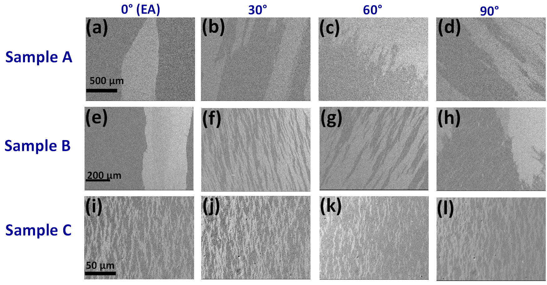
Figure 2: Domain images captured for samples A, B and C at angles, 0^∘, 30^∘, 60^∘ and 90^∘ near to coercivity are shown. Scale bars are shown on the domain images for each sample separately which are valid for the images recorded at other angles for those respective samples.

Domain images captured near to coercive field H_C for all three samples at 0^∘, 30^∘, 60^∘ and 90^∘ are displayed in figure 2. The black and gray contrast in the domain images represent positive and negative magnetized states, respectively. From the domain images it can be concluded that magnetization reversal occurs via domain wall motion. Sample A (figure 2 a to d) exhibits large well-defined stripe domains which indicates the presence of weak magnetic anisotropy. These stripe domains are found to be tilted for e.g. $\Phi$ = 30^∘ and 60^∘ (figure 2 b and c). For $\Phi$ = 90^∘ (figure 2d) branched domains are observed. In addition to 180^∘ domain wall, sample B (figure 2 e to h) shows 90^∘ domain walls at certain angles of measurement (figure S1). Sample C (figure 2 i to l) shows narrow branched domains and are found to be independent of $\Phi$ , which indicates that the sample C is magnetically isotropic in nature. By comparing the domain images at any particular $\Phi$ among the samples, it is observed that the size (i.e. width) of the domain decreases with increasing anisotropy strength.

In the following we have investigated the magnetization dynamics of the $\textit{L}1_{0}$–FeNi films by FMR. Measured FMR spectra (open symbol) for samples A and C at selective frequencies are shown in figure 3 (a) and (b), respectively. Resonance field (H_res) and line width ($\Delta H$) were extracted by fitting of Lorentzian shape function (equation 1) having anti-symmetric (first term) and symmetric components (second term) to the obtained FMR derivative signal Singh et al. (2017);

$$\begin{split}S_{21}&=K_{1}\frac{4\Delta H(H-H_{res})}{[4(H-H_{res})^{2}+(\Delta H)^{2}]^{2}}\\ &-K_{2}\frac{(\Delta H)^{2}-4(H-H_{res})^{2}}{[4(H-H_{res})^{2}+(\Delta H)^{2}]^{2}}\\ &+(slopeH)+Offset\end{split}$$ (1)

where S₂₁ is transmission signal, K₁ and K₂ are coefficient of anti-symmetric and symmetric component, respectively, slope H is drift value in amplitude of the signal. Frequency (f) dependence of H_res and $\Delta$H are plotted in figure 3 (a) and (b), respectively. From the f vs. H_res plot, parameters such as Lande g-factor, effective demagnetization field (4$\pi$M_eff), anisotropy field H_K were extracted by fitting it to Kittel resonance condition Kittel (1948);

$$f=\frac{\gamma}{2\pi}\sqrt{(H_{K}+H_{res})(H_{K}+H_{res}+4\pi M_{eff})}$$ (2)

where $\gamma=g\mu_{B}/\hbar$ is gyromagnetic ratio, $\mu_{B}$ as Bohr magneton, $\hbar$ as reduced Planck’s constant. The values of damping constant $\alpha$ for all three samples were extracted by using the equation Singh et al. (2017); Kittel (1948); Heinrich et al. (1985);

$$\Delta H=\Delta H_{0}+\frac{4\pi\alpha f}{\gamma}$$ (3)

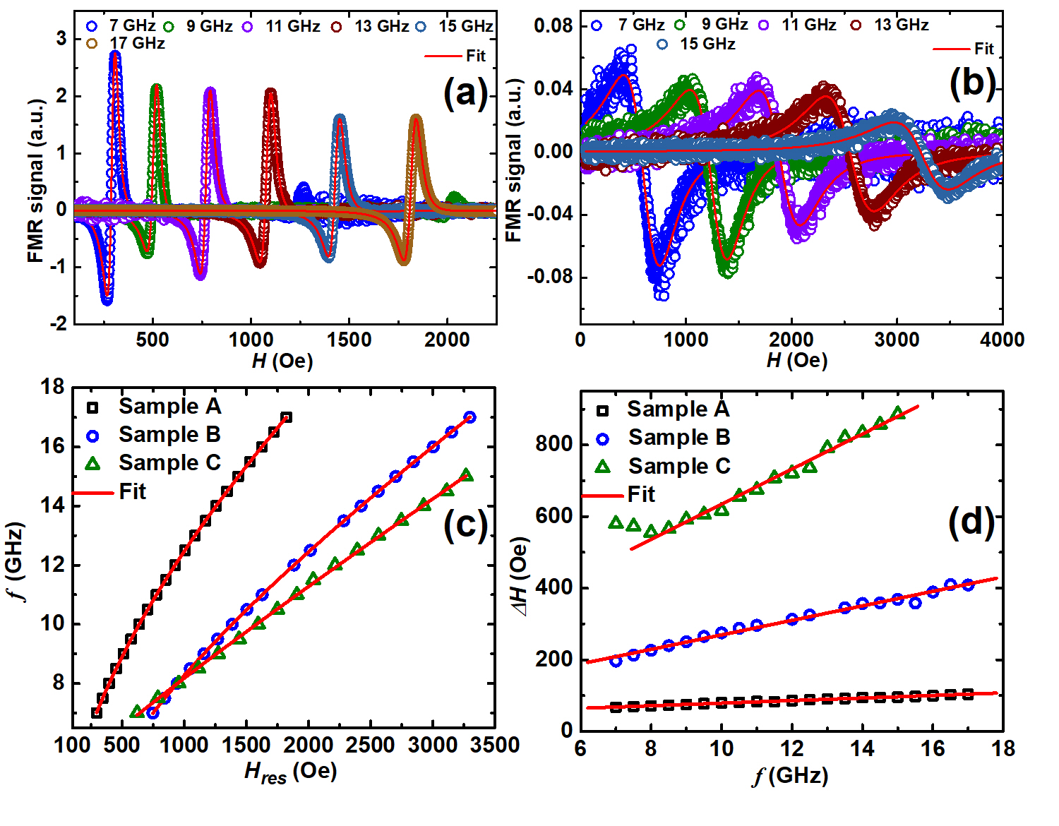
Figure 3: FMR spectra of (a) sample A and (b) sample C measured at frequency 5 – 17 GHz. The solid lines in (a) and (b) are fitted with equation 1. (c) f vs. H_res and (d) $\Delta H$ vs. f plots for samples A – C extracted from the FMR frequency dependent spectra. The lines in (c) and (d) are the best fits to the equations (2) and (3), respectively.

Table 1: The Parameters extracted from the fitting of FMR experimental data (Figure 3) of all three samples using the equations (2) and (3)

Sample	HK(Oe)	$4\pi M_{eff}$	g-factor	$\alpha$	$\Delta$ H0(Oe)
A	49.41$\pm$0.82	18279$\pm$365	1.97$\pm$0.01	0.0049$\pm$0.0001	42.85$\pm$0.65
B	-52.39$\pm$4.64	8900$\pm$193	1.93$\pm$0.01	0.0277$\pm$0.0007	66.89$\pm$7.13
C	680.29$\pm$106.88	3509$\pm$106	1.98$\pm$0.01	0.0680$\pm$0.0019	143.67$\pm$16.20

where $\Delta H_{0}$ is called as inhomogeneous line width broadening. Values of all the fitting parameters obtained by using equations (1) and (2) are given in table 1. With increase in anisotropy strength of the samples, $4\pi M_{eff}$ decreases whereas $\alpha$ increases. Sample A exhibits lowest value of $\alpha$, $4.9\times 10^{-3}$ which is the same order with normal FeNi alloy thin film ($\alpha=1.2\times 10^{-3}$) Zhu et al. (2018). The value of inhomogeneous line width broadening $\Delta H_{0}$, which depends on the quality of the thin film Singh et al. (2017), is highest for sample C and lowest for sample A.

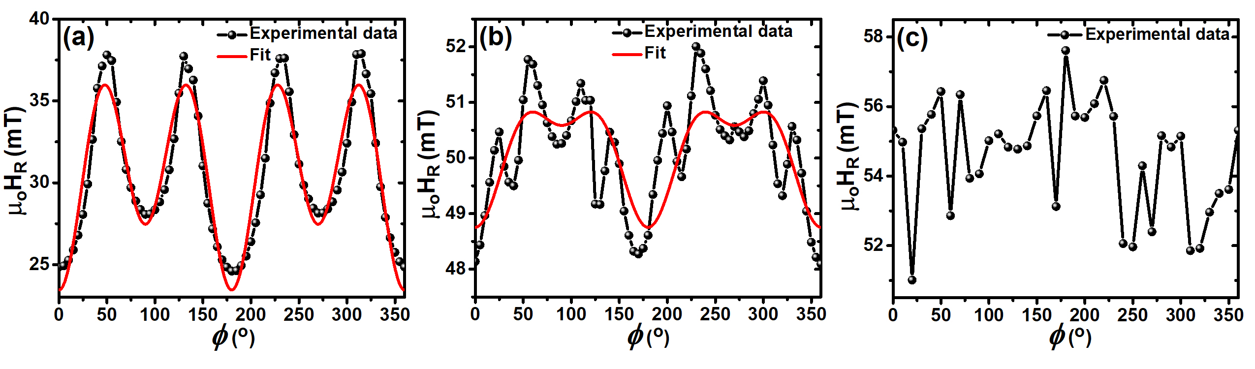
Figure 4: Anisotropy symmetry plot and the fits for (a) sample A, (b) sample B and (c) sample C measured using FMR by keeping the frequency fixed at 7 GHz. The red solid lines are the best fits to equation (4).

Apart from frequency dependent FMR, angle dependent FMR measurements at a fixed frequency of 7 GHz were performed to analyze the anisotropy energy density as well as symmetry of all three samples. Figure 4 shows the angle dependent H_res plot for all three samples. Samples A and B clearly show the presence of mixed cubic and uniaxial anisotropies with minima in H_res approximately at angles 0^∘, 90^∘, 180^∘ and 270^∘. From the angle dependent H_res plot, the value of uniaxial and cubic anisotropy energy constants have been estimated by fitting those data to solution of LLG equation that includes the cubic and uniaxial anisotropies and it is written as Pan et al. (2017);

$$\begin{split}f&=\frac{\gamma}{2\pi}\left[H+\frac{2K_{2}}{M_{s}}cos2\phi-\frac{4K_{4}}{M_{s}}cos4\phi\right]\\ &\times\left[H+4\pi M_{s}+\frac{2K_{2}}{M_{s}}cos2\phi-\frac{K_{4}}{M_{s}}(3+cos4\phi)\right]^{1/2}\end{split}$$ (4)

Table 2: The parameters extracted from the fitting of angle dependent FMR experimental data of two samples using the equation (4)

Samples	$M_{s}$(emu cm-3)	$K_{2}$(erg cm-3)	$K_{4}$(erg cm-3)
A	1645	1.66$\times$104	-2.16$\times$104
B	1026.8	4.8$\times$103	-1.2$\times$103
C	Magnetically isotropic behaviour

where, K₂ and K₄ are cubic and uniaxial anisotropy energy density constants, respectively, M_S is saturation magnetization, H is the applied magnetic field, $\Phi$ is the angle between applied field direction and easy axis of the sample. The angle dependence of H_res is fitted to equation 4. From the fit, value of M_S, K₂ and K₄ have been extracted and are shown in table 2. It has been found that both cubic and uniaxial anisotropy energy constants of sample A are greater than that of sample B by one order of magnitude. Further in sample A the ratio between the cubic to uniaxial anisotropy is about  0.75 whereas for sample B the ratio is 4. Therefore for sample B the cubic anisotropy is four times stronger than the uniaxial anisotropy. This is the reason of occurrence of 90^∘ domain walls for sample B as shown in Fig. S1Mallik et al. (2014). In comparison to samples A and B, sample C shows isotropic behavior which is in consistent with the results obtained from Kerr microscopy.

$\textit{L}1_{0}$-FeNi thin films (samples A, B and C) show different strength of anisotropy, which were fabricated by different deposition processes in a MBE system. Domain images reveals that magnetization reversal for all three samples occur via nucleation and subsequent domain wall motion. We have observed lowest values of $\alpha$ $\sim$ $4.9\times 10^{-3}$ for the sample A which shows moderate magnetic anisotropy. Angle dependent FMR measurement shows the mixed cubic and uniaxial anisotropy in samples A and B, while sample C exhibits magnetically isotropic behavior. Our work demonstrates that variable anisotropic $\textit{L}1_{0}$-FeNi thin films can be fabricated in which the damping constant and magnetization reversal can be tuned. These results may be useful for future spintronics based applications.

Acknowledgements: We acknowledge the financial support by department of atomic energy (DAE), Department of Science and Technology (DST-SERB) of Govt. of India,DST-Nanomission (SR/NM/NS-1018/2016(G)) and DST, government of India for INSPIRE fellowship.

References

Supplementary Material

Figure 5: Magnetic domain images for sample B at various fields close to the reversal field. It shows that the magnetization reversal is happening through 90^∘ domain wall in sample B.

References

- Bandic and Victora (2008) Z. Z. Bandic and R. H. Victora, Proceedings of the IEEE 96, 1749 (2008).
- Bedanta and Kleemann (2008) S. Bedanta and W. Kleemann, Journal of Physics D: Applied Physics 42, 013001 (2008).
- Weller and Moser (1999) D. Weller and A. Moser, IEEE Transactions on magnetics 35, 4423 (1999).
- Kotsugi et al. (2013) M. Kotsugi, M. Mizuguchi, S. Sekiya, M. Mizumaki, T. Kojima, T. Nakamura, H. Osawa, K. Kodama, T. Ohtsuki, T. Ohkochi, et al., Journal of Magnetism and Magnetic Materials 326, 235 (2013).
- Goto et al. (2017) S. Goto, H. Kura, E. Watanabe, Y. Hayashi, H. Yanagihara, Y. Shimada, M. Mizuguchi, K. Takanashi, and E. Kita, Scientific reports 7, 13216 (2017).
- Klemmer et al. (2003) T. Klemmer, C. Liu, N. Shukla, X. Wu, D. Weller, M. Tanase, D. Laughlin, and W. Soffa, Journal of magnetism and magnetic materials 266, 79 (2003).
- Kojima et al. (2014) T. Kojima, M. Ogiwara, M. Mizuguchi, M. Kotsugi, T. Koganezawa, T. Ohtsuki, T.-Y. Tashiro, and K. Takanashi, Journal of Physics: Condensed Matter 26, 064207 (2014).
- Takanashi et al. (2017) K. Takanashi, M. Mizuguchi, T. Kojima, and T. Tashiro, Journal of Physics D: Applied Physics 50, 483002 (2017).
- Mizuguchi et al. (2010) M. Mizuguchi, S. Sekiya, and K. Takanashi, Journal of Applied Physics 107, 09A716 (2010).
- Kotsugi et al. (2011) M. Kotsugi, M. Mizuguchi, S. Sekiya, T. Ohkouchi, T. Kojima, K. Takanashi, and Y. Watanabe, in Journal of Physics: Conference Series, Vol. 266 (IOP Publishing, 2011) p. 012095.
- Mibu et al. (2015) K. Mibu, T. Kojima, M. Mizuguchi, and K. Takanashi, Journal of Physics D: Applied Physics 48, 205002 (2015).
- Ogiwara et al. (2013) M. Ogiwara, S. Iihama, T. Seki, T. Kojima, S. Mizukami, M. Mizuguchi, and K. Takanashi, Applied Physics Letters 103, 242409 (2013).
- Kojima et al. (2011) T. Kojima, M. Mizuguchi, T. Koganezawa, K. Osaka, M. Kotsugi, and K. Takanashi, Japanese Journal of Applied Physics 51, 010204 (2011).
- (14) “EVICOmagnetics,” http://www.evico-magnetics.de/microscope.html.
- (15) “NanOsc FMR Spectrometers,” https://www.qdusa.com/products/nanosc-fmr-spectrometers.html.
- Mallick et al. (2014) S. Mallick, S. Bedanta, T. Seki, and K. Takanashi, Journal of Applied Physics 116, 133904 (2014).
- Singh et al. (2017) B. B. Singh, S. K. Jena, and S. Bedanta, Journal of Physics D: Applied Physics 50, 345001 (2017).
- Kittel (1948) C. Kittel, Physical Review 73, 155 (1948).
- Heinrich et al. (1985) B. Heinrich, J. Cochran, and R. Hasegawa, Journal of Applied Physics 57, 3690 (1985).
- Zhu et al. (2018) Z. Zhu, H. Feng, X. Cheng, H. Xie, Q. Liu, and J. Wang, Journal of Physics D: Applied Physics 51, 045004 (2018).
- Pan et al. (2017) S. Pan, T. Seki, K. Takanashi, and A. Barman, Physical Review Applied 7, 064012 (2017).
- Mallik et al. (2014) S. Mallik, N. Chowdhury, and S. Bedanta, AIP Advances 4, 097118 (2014).