Multiple stellar populations: from old Milky Way globulars to young star clusters

Abstract

I present the latest results from our group about the multiple stellar populations in the old Milky Way globular clusters (GCs) and in the young systems both in the Magellanic Clouds and in the Milky Way. For the ancient GCs in our Galaxy I summarize the chemical properties of the stellar populations as observed on the chromosome map. Both Type I and Type II GCs are discussed. For the youngest clusters I will briefly report our latest spectroscopic analysis on the Large Magellanic Cloud cluster NGC 1818 and the Galactic open cluster M 11, which supports the co-existence of stellar populations with different rotation rates.

1 Introduction

The presence of more than one stellar population in globular clusters (GCs) is one of the most fascinating discovery in the field of stellar populations in the last decade. The definition itself of a GC as the prototype of a Simple Stellar Population (SSP), definitively shattered out. One of the direct consequences of the failure of the SSP assumption is that stellar evolutionary models, which use GCs as calibrators, need to be updated. Furthermore, the properties of stellar populations in these ancient stellar systems provide important information on the Universe at its earliest phases and on the assembly of the Milky Way (MW) halo. Despite the crucial role played by the presence of more than one stellar populations in GCs, and the numerous scenarios proposed, at present none of them is able to properly account for all the observational constraints (see [Renzini et al.(2015), Renzini et al. 2015] for a critical discussion).

Star formation theory assumes that typically stars do not form in isolation, but in clusters and associations, eventually dissolving. Star clusters formed along almost the whole timeline of Universe history, with ancient GCs, like those in the MW, being among the oldest objects in the Universe. Star clusters continue forming and a rich population of young and intermediate-age objects are observed in the Magellanic Clouds galaxies.

From an observational perspective, the multiple stellar populations phenomenon is mostly constrained in the ancient MW GCs, that formed between $\sim$13 and 10 Gyrs ago. Some hints of different stellar populations are also observed in intermediate-age objects in the Magellanic Clouds. In this context, very young clusters are interesting objects because they could potentially provide a window, in the Local Universe, to observe a poorly-understood phenomenon occurred at high redshift. The basic question to answer is if the multiple stellar populations are indeed multiple generations of stars, and if star clusters could have supported more than one burst of star formation.

In the following, I will summarize the latest observational results on multiple stellar populations in the old MW GCs (Sections 2 and 3), and in some younger systems both in the Large Magellanic Cloud and in the MW (Section 4).

2 Chemical signatures from the ChMs

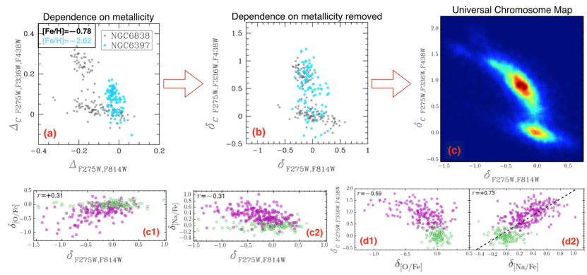
Figure 1: The universal ChM of GCs ([Marino et al.(2019), Marino et al. 2019]). Panels (a) and (b) illustrate the original maps ($\Delta_{\tiny{C~{}\mathrm{F275W,F336W,F438W}}}$ vs. $\Delta_{\tiny{\mathrm{F275W,F814W}}}$), which are metallicity-dependent, and the final maps used to construct the universal map ($\delta_{\tiny{C~{}\mathrm{F275W,F336W,F438W}}}$ vs. $\delta_{\tiny{\mathrm{F275W,F814W}}}$), where the metallicity dependence has been removed. The final universal map is displayed in panel (c). Panels (c1) and (c2) show the abundance ratios of O and Na relative to the average abundances of 1G stars vs. the $\delta_{\tiny{\mathrm{F275W,F814W}}}$. Panels (d1) and (d2) represent $\delta_{\tiny{C~{}\mathrm{F275W,F336W,F438W}}}$ as a function of the same abundance ratios. In panels (c1)-(c2)-(d1)-(d2) 1G and 2G stars are represented in green and magenta, respectively. For each element, we report the Spearman’s correlation coefficient $r$, and in panel (d2) we plot the least-square fit with data.

Central to the characterization of the different stellar populations in GCs, and for our understanding of this complex phenomenon, is the knowledge of chemical abundances. Recently, [Milone et al.(2015), Milone et al. (2015)] have introduced one very effective way of visualizing the complexity of multiple stellar populations by means of a diagnostic diagram dubbed chromosome map (ChM), with such maps having been presented for 58 GCs ([Milone et al.(2017), Milone et al. 2017]). In the ChM plot ($\Delta_{\tiny{C~{}\mathrm{F275W,F336W,F438W}}}$ vs. $\Delta_{\tiny{\mathrm{F275W,F814W}}}$) GCs stars are typically separated into two distinct groups: one first-population (1G) group and a second-population (2G) one. Specifically, 1G stars are located around the origin of the ChM (i.e., $\Delta_{\tiny{C~{}\mathrm{F275W,F336W,F438W}}}$=$\Delta_{\tiny{\mathrm{F275W,F814W}}}$=0), while 2G stars have large $\Delta_{\tiny{C~{}\mathrm{F275W,F336W,F438W}}}$ and low $\Delta_{\tiny{\mathrm{F275W,F814W}}}$.

One of the most surprising features of the multiple populations phenomenon, as seen from the ChMs, is its variety. GCs host different number of stellar populations, with the extension and morphology of the map changing from one cluster to another. With the aim of trying to find some global pattern among the multiple populations on the ChM and chemical abundance and investigate possible common properties in such a variegate zoo, in [Marino et al.(2019), Marino et al. (2019)] we attempted a comparison of ChMs of different GCs. To this goal we first had to obtain comparable maps, removing their dependence on metallicity.

The $\Delta_{\tiny{C~{}\mathrm{F275W,F336W,F438W}}}$ and $\Delta_{\tiny{\mathrm{F275W,F814W}}}$ width of the ChM dramatically changes from one cluster to another and mostly correlates with the cluster metallicity. An example of this dependence is represented in panel (a) of Fig. 1. While both the plotted GCs exhibit a quite simple ChM, the ChM extension of the metal-richer cluster (NGC 6838) is significantly wider than that of NGC 6397, which has a much lower metallicity. After removing this dependence, as explained in [Marino et al.(2019), Marino et al. (2019)], we move to a plane ($\delta_{\tiny{C~{}\mathrm{F275W,F336W,F438W}}}$ vs. $\delta_{\tiny{\mathrm{F275W,F814W}}}$) where stellar populations in clusters at different metallicity can be easily compared (panel (b)).

By combining all the available ChMs in the metal-free plane (excluding red populations in Type II GCs which will be discussed in the next section), we get a “Universal ChM of multiple stellar populations in GCs”. Panel (c) displays this universal map as a Hess diagram, indicative of the density of all the stars. The analysis of the main pattern appearing on the universal ChM has provided information on the global properties of the multiple stellar populations phenomenon in GCs. On top of the high degree of variety, the universal map displays: (1) two major over-densities of stars, one on the 1G and the other on the 2G; (2) a clear separation between 1G and 2G stars that occurs to $\Delta_{\tiny{C~{}\mathrm{F275W,F336W,F438W}}}\sim$0.25; (3) the first over-density, the 1G population, appears to occupy a relatively narrow range in $\Delta_{\tiny{C~{}\mathrm{F275W,F336W,F438W}}}$. The extension in $\Delta_{\tiny{\mathrm{F275W,F814W}}}$ is larger, but most stars are located within $-$0.3$<\Delta_{\tiny{\mathrm{F275W,F814W}}}<+$0.3; (4) the bulk of 2G stars are clustered around $\Delta_{\tiny{C~{}\mathrm{F275W,F336W,F438W}}}\sim$0.9 with a poorly-populated tail of stars extended towards larger values. This suggests that even if the ChMs is variegate, the dominant 2G in GCs has similar properties.

The obvious question here is: how this is related to the chemical composition of stellar populations? The most studied (and distinctive) chemical pattern in GCs is the Na-O anticorrelation (e.g. [Carretta et al.(2009), Carretta et al. 2009]). The universal ChM allowed us to investigate the global variations in light elements in the overall sample of analyzed GCs.

In panels (c1) and (c2) of Fig. 1 we plot the abundance ratios of O and Na relative to the average abundances of 1G stars ($\delta_{\tiny{\mathrm{[O/Fe]}}}$ and $\delta_{\tiny{\mathrm{[Na/Fe]}}}$) as a function of $\delta_{\tiny{\mathrm{F275W,F814W}}}$. We note that overall the 2G stars have enhanced Na (higher $\delta_{\tiny{\mathrm{[Na/Fe]}}}$), and most stars are depleted in O (lower $\delta_{\tiny{\mathrm{[O/Fe]}}}$). Interestingly, despite the large range spanned in $\delta_{\tiny{\mathrm{F275W,F814W}}}$, 1G stars have constant chemical abundance both in O and Na.

Panels (d1) and (d2) represent $\delta_{\tiny{C~{}\mathrm{F275W,F336W,F438W}}}$ as a function of $\delta_{\tiny{\mathrm{[O/Fe]}}}$ and $\delta_{\tiny{\mathrm{[Na/Fe]}}}$. We find a significant correlation with $\delta_{\tiny{\mathrm{[Na/Fe]}}}$. An anticorrelations is present between $\delta_{\tiny{C~{}\mathrm{F275W,F336W,F438W}}}$ and $\delta_{\tiny{\mathrm{[O/Fe]}}}$.

While I refer to [Marino et al.(2019), Marino et al. (2019)] for a detailed chemical characterization of the GC ChMs, here I emphasize that the presented analysis demonstrates the power of the ChM to disentangle between stars with different chemical abundances. Hence, individual ChMs and the universal ChM are, at present, the best tools available to explore the multiple stellar population phenomenon and the nature of the different populations hosted in GCs.

3 Signatures of heavy element variations

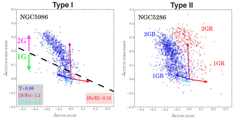
Figure 2: ChMs of the Type I GC NGC 5986 and the Type II GC NGC 5286. The arrows indicate the effect of changing He, N, O, and Fe by the quoted quantities. The diagram of Type II GCs shows additional maps (1GR and 2GR) on the red side of the main map (1GB and 2GB). The dashed line on the left panel separates 1G from 2G stars.

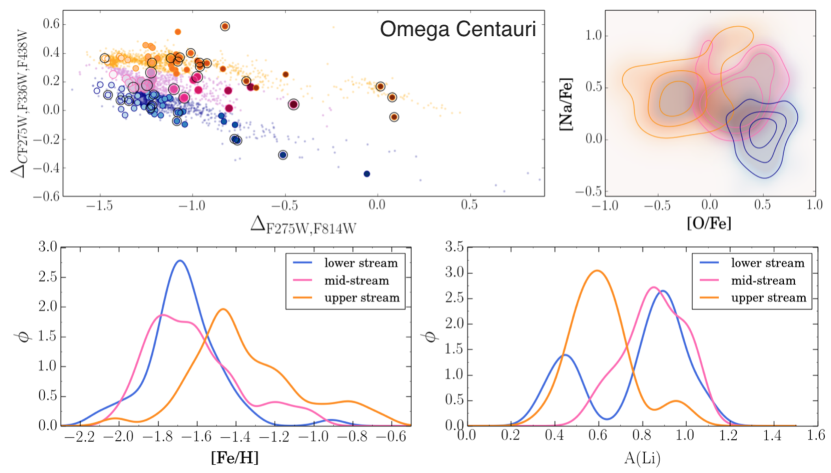
Figure 3: Top-left panel: ChM of $\omega$ Centauri. The lower, middle, and upper streams have been coloured in light blue, pink and orange, respectively. Larger dots are stars with abundances from [Johnson & Pilachowski(2010), Johnson & Pilachowski (2010)] and [Marino et al.(2011), Marino et al. (2011)] (black-circled points). To each star with abundances a gradient in colour has been assigned proportional to its $\Delta_{\tiny{\mathrm{F275W,F814W}}}$. Top-right panel: density levels on the Na-O plane for stars belonging to each stream. Lower panels: Gaussian kernel density distributions of [Fe/H] and A(Li) for the streams by using the [Johnson & Pilachowski(2010), Johnson & Pilachowski (2010)], [Marino et al.(2011), Marino et al. (2011)] and [Mucciarelli et al.(2018), Mucciarelli et al. (2018)] samples.

The variety of the multiple populations phenomenon has prompted efforts to classify GCs in different classes, whose definition has changed from time to time, depending on the new features being discovered. [Milone et al.(2017), Milone et al. (2017)] subdivided the analyzed ChMs in two main groups: (i) Type I GCs having a single ChM pattern, with a 1G and two or more 2G populations, and (ii) Type II GCs displaying multiple ChMs, with minor populations located on red additional ChMs. The “Type II phenomenon” occurs in $\sim$17% of the analyzed clusters, and suggests that these objects have experienced a much more complex star formation history.

In Fig. 2 I show the ChMs of a typical Type I GC, NGC 5986, and a typical Type II one, NGC 5286. Other examples of Type II GCs are M 22, M 2, NGC 6934, and $\omega$ Centauri. The analysis of the effect of variations in chemical elements on the map, clearly shows that the increase in the $\Delta_{\tiny{C~{}\mathrm{F275W,F336W,F438W}}}$ index is primarily due to nitrogen enhancements, while helium increases with decreasing $\Delta_{\tiny{\mathrm{F275W,F814W}}}$ ([Milone et al.(2015), Milone et al. 2015]).

The $\Delta_{\tiny{\mathrm{F275W,F814W}}}$ index is sensitive to the overall metallicity, suggesting that stars on the red sequences of the map are enhanced in [Fe/H]. Indeed, all the GCs with known variations in iron belong to this (photometrically defined) class of objects (e.g. [Marino et al.(2018a), Marino et al. 2018]). In most of these clusters, internal variations in $slow$-neutron capture elements correlate with the enhancement in metals (e.g. [Marino et al.(2015), Marino et al. 2015]). The reason why this different chemical behavior occurs remains to be established, but, intriguingly, might be linked to a different origin with respect to the more common GCs in the Galaxy (see discussion in [Marino et al.(2019), Marino et al. 2019]).

Omega Centauri, with its well-documented large variations in metallicity, is the most extreme example of a Type II GC. We have explored in details the ChM of this GC, whose wide ranges in chemical abundances make it an ideal laboratory to test the role of each element in shaping the GC ChMs.

In Fig. 3 three main streams of stars are evident at different levels of $\Delta_{\tiny{C~{}\mathrm{F275W,F336W,F438W}}}$. The upper stream stars mostly occupy the section of higher Na and lower O quadrant of the O-Na plane with [O/Fe]$<$0.0 dex. Mid-stream stars mostly distribute on a intermediate location in the O-Na plane, while lower stream stars have lower Na and higher O. As a general rule, stellar populations with increasing Fe populate redder and redder regions of the map. The Fe enrichment seems generally de-coupled from the light-elements processing. The lower and mid-streams are peaked at similar Fe ([Fe/H]$\sim-$1.7 dex), with the mid-stream having a minor over-density of stars at higher Fe. The upper stream is the most distinct: it is peaked on higher metallicity and lower Li abundances. As the upper-stream red-RGB stars have a more extreme enrichment in Na and Al, and depletion in Li and O, these stars are likely the most-enhanced in helium.

This discussion highlights the efficiency of the ChMs in separating stars with different chemical content in heavy elements. This diagnostic tool can be exploited to identify GCs with variations in the overall metallicity. A chemical abundance exploration of the ChM of $\omega$ Centauri suggests that the most important Fe-enrichment occurred when the intra-cluster medium was already extremely enriched in He and in H-burning products.

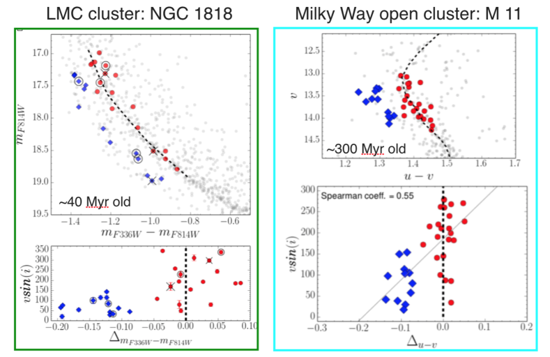
Figure 4: Left panels: $m_{\mathrm{F}814W}$-$(m_{\mathrm{F}336W}-m_{\mathrm{F}814W})$ CMD of the LMC cluster NGC 1818 zoomed-in on the split MS. The black dashed line is a fiducial for the rMS (upper panel). The lower panel shows $v$sin$i$ as a function of the difference between the $m_{\mathrm{F}336W}-m_{\mathrm{F}814W}$ color of each MS star and the color of the fiducial ($\Delta_{m_{\mathrm{F}336W}-m_{\mathrm{F}814W}}$). The circle and cross symbols indicate SB1 candidates and stars with H$\alpha$ core and/or wings emissions, respectively. Right panels: $v$-$(u-v)$ CMD of the open cluster M 11 zoomed-in on the split MS. The black dashed line is a fiducial for the rMS. $v$sin$i$ as a function of the difference between the $u-v$ color of each MS star and the color of the fiducial ($\Delta_{u-v}$) is shown in the lower panel. In all the plots, rMS and bMS stars are represented with red filled circles and blue diamonds, respectively.

4 Young clusters in the Magellanic Clouds and the Milky Way

It seems that multiple stellar populations are not a peculiarity of the old Galactic GCs. Indeed, split main sequences (MSs) and extended MS turn-offs (eMSTOs) have been discovered along the color-magnitude diagrams (CMDs) of young (age $\sim$50-500 Myr) clusters in both Magellanic Clouds (e.g. [Milone et al.(2016), Milone et al. 2016]). Despite a huge effort has been undertaken to understand these observations, the physical mechanism responsible for the eMSTO is still obscure.

The eMSTO has been originally interpreted as due to an age spread of 50-500 Myrs; in such a case the clusters with the eMSTO would be the younger counterparts of the old GCs with multiple populations ([Mackey, & Broby Nielsen(2007), Mackey & Broby Nielsen 2007]). Another interpretation is that the eMSTO is an effect of stellar rotation (e.g. [Bastian, & de Mink(2009), Bastian & de Mink 2009]).

We have reported the first direct spectroscopic measurements of projected rotational velocities ($v$sin$i$) for the double MS, and eMSTO in a Large Magellanic Cloud (LMC) cluster, namely NGC 1818 ([Marino et al.(2018b), Marino et al. 2018b]). Figure 4 shows that the blue-MS (bMS) is populated by slowly rotating stars, while the red-MS (rMS) is composed of fast rotators, with rotation close to the breaking speed (left panel of Fig. 4). Similar multiple sequences are observed in the Milky Way open clusters at similar ages ([Marino et al.(2018c), Marino et al. 2018c]; [Cordoni et al.(2018), Cordoni et al. 2018]). Also in the Milky Way, this phenomenon is associated to stellar populations with different rotation (right panel of Fig. 4; [Marino et al.(2018c), Marino et al. 2018c]). These observations suggest that multiple sequences in young clusters are populated by stars with different rotation, and we might not need an age spread to reproduce the observed CMDs.

References

- [Bastian, & de Mink(2009)] Bastian, N., & de Mink, S. E. 2009, MNRAS, 398, L11
- [Carretta et al.(2009)] Carretta, E., Bragaglia, A., Gratton, R. G., et al. 2009, A&A, 505, 117
- [Cordoni et al.(2018)] Cordoni, G., Milone, A. P., Marino, A. F., et al. 2018, ApJ, 869, 139
- [Johnson & Pilachowski(2010)] Johnson, C. I., & Pilachowski, C. A. 2010, ApJ, 722, 1373
- [Mackey, & Broby Nielsen(2007)] Mackey, A. D., & Broby Nielsen, P. 2007, MNRAS, 379, 151
- [Marino et al.(2011)] Marino, A. F., Milone, A. P., Piotto, G., et al. 2011, ApJ, 731, 64
- [Marino et al.(2015)] Marino, A. F., Milone, A. P., Karakas, A. I., et al. 2015, MNRAS, 450, 815
- [Marino et al.(2018a)] Marino, A. F., Yong, D., Milone, A. P., et al. 2018a, ApJ, 859, 81
- [Marino et al.(2018b)] Marino, A. F., Przybilla, N., Milone, A. P., et al. 2018b, AJ, 156, 116
- [Marino et al.(2018c)] Marino, A. F., Milone, A. P., Casagrande, L., et al. 2018, ApJ, 863, L33
- [Marino et al.(2019)] Marino, A. F., Milone, A. P., Renzini, A., et al. 2019, MNRAS, 487, 3815
- [Milone et al.(2015)] Milone, A. P., Marino, A. F., Piotto, G., et al. 2015, MNRAS, 447, 927
- [Milone et al.(2016)] Milone, A. P., Marino, A. F., D’Antona, F., et al. 2016, MNRAS, 458, 4368
- [Milone et al.(2017)] Milone, A. P., Piotto, G., Renzini, A., et al. 2017, MNRAS, 464, 3636
- [Mucciarelli et al.(2018)] Mucciarelli, A., Salaris, M., Monaco, L., et al. 2018, A&A, 618, A134
- [Renzini et al.(2015)] Renzini, A., D’Antona, F., Cassisi, S., et al. 2015, MNRAS, 454, 4197