Semiclassical inverse spectral problem for elastic Rayleigh waves in isotropic media

Abstract

We analyze the inverse spectral problem on the half line associated with elastic surface waves. Here, we extend the treatment of Love waves [6] to Rayleigh waves. Under certain conditions, and assuming that the Poisson ratio is constant, we establish uniqueness and present a reconstruction scheme for the S-wave speed with multiple wells from the semiclassical spectrum of these waves.

1 Introduction

We analyze the inverse spectral problem on the half line associated with elastic surface waves. We discussed Love waves in a previous paper [6], and in this paper we analyze this inverse problem for Rayleigh waves.

We study the elastic wave equation in $X={\mathbb{R}}^{2}\times(-\infty,0]$. In coordinates,

$$(x,z),\quad x=(x_{1},x_{2})\in{\mathbb{R}}^{2},\ z\in{\mathbb{R}}^{-}=(-\infty,0],$$

we consider solutions, $u=(u_{1},u_{2},u_{3})$, satisfying the Neumann boundary condition at $\partial X=\{z=0\}$, to the system

(1) $$\begin{split}\partial^{2}_{t}u_{i}+M_{il}u_{l}&=0,\\ u(t=0,x,z)&=0,~{}~{}\partial_{t}u(t=0,x,z)=h(x,z),\\[-2.84544pt] \frac{c_{i3kl}}{\rho}\partial_{k}u_{l}(t,x,z=0)&=0,\end{split}$$

where

$$M_{il}=-\frac{\partial}{\partial z}\frac{c_{i33l}(x,z)}{\rho(x,z)}\frac{\partial}{\partial z}-\sum_{j,k=1}^{2}\frac{c_{ijkl}(x,z)}{\rho(x,z)}\frac{\partial}{\partial x_{j}}\frac{\partial}{\partial x_{k}}-\sum_{j=1}^{2}\frac{\partial}{\partial x_{j}}\frac{c_{ij3l}(x,z)}{\rho(x,z)}\frac{\partial}{\partial z}\\ -\sum_{k=1}^{2}\frac{c_{i3kl}(x,z)}{\rho(x,z)}\frac{\partial}{\partial z}\frac{\partial}{\partial x_{k}}-\sum_{k=1}^{2}\left(\frac{\partial}{\partial z}\frac{c_{i3kl}(x,z)}{\rho(x,z)}\right)\frac{\partial}{\partial x_{k}}-\sum_{j,k=1}^{2}\left(\frac{\partial}{\partial x_{j}}\frac{c_{ijkl}(x,z)}{\rho(x,z)}\right)\frac{\partial}{\partial x_{k}}.$$

Here, the stiffness tensor, $c_{ijkl}$, and density, $\rho$, are smooth and obey the following scaling: Introducing $Z=\frac{z}{\epsilon}$,

$$\frac{c_{ijkl}}{\rho}(x,z)=C_{ijkl}\left(x,\frac{z}{\epsilon}\right),~{}~{}\epsilon\in(0,\epsilon_{0}];$$

$$C_{ijkl}(x,Z)=C_{ijkl}(x,Z_{I})=C_{ijkl}^{I}(x),\quad Z\leqslant Z_{I}<0.$$

As discussed in [5], surface waves travel along the surface $z=0$.

The remainder of the paper is organized as follows. In Section 2, we give the formulation of the inverse problems as an inverse spectral problem on the half line and treat the simple case of recovery of a monotonic wave-speed profile. In Section 3, we discuss the relevant Bohr-Sommerfeld quantization, which is the main result of this paper as it forms the key component in the study of the inverse spectral problem. In Section 4, we give the reconstruction scheme under appropriate assumptions, which is an adaptation of the method of Colin de Verdière [4].

2 Semiclassical description of Rayleigh waves

2.1 Surface wave equation, trace and the data

We briefly summarize the semiclassical description of elastic surface waves [5]. The leading-order symbol associated with $M_{il}$ above is given by

(2) $$H_{0,il}(x,\xi)=-\frac{\partial}{\partial Z}C_{i33l}(x,Z)\frac{\partial}{\partial Z}\\ -\mathrm{i}\sum_{j=1}^{2}C_{ij3l}(x,Z)\xi_{j}\frac{\partial}{\partial Z}-\mathrm{i}\sum_{k=1}^{2}C_{i3kl}(x,Z)\frac{\partial}{\partial Z}\xi_{k}-\mathrm{i}\sum_{k=1}^{2}\left(\frac{\partial}{\partial Z}C_{i3kl}(x,Z)\right)\xi_{k}\\ +\sum_{j,k=1}^{2}C_{ijkl}(x,Z)\xi_{j}\xi_{k}.\hskip 113.81102pt$$

We view $H_{0}(x,\xi)$ as an ordinary differential operator in $Z$, with domain

$$\mathcal{D}=\left\{v\in H^{2}(\mathbb{R}^{-})\ \bigg{|}\ \sum_{l=1}^{3}\left(C_{i33l}(x,0)\frac{\partial v_{l}}{\partial Z}(0)+\mathrm{i}\sum_{k=1}^{2}C_{i3kl}\xi_{k}v_{l}(0)\right)=0\right\}.$$

For an isotropic medium we have

$$C_{ijkl}=\hat{\lambda}\delta_{ij}\delta_{kl}+\hat{\mu}(\delta_{ik}\delta_{jl}+\delta_{il}\delta_{jk}),$$

where $\hat{\lambda}=\frac{\lambda}{\rho},$ $\hat{\mu}=\frac{\mu}{\rho}$, and $\lambda,\mu$ are the two Lamé moduli. The P-wave speed, $C_{P}$, is then $C_{P}=\sqrt{\hat{\lambda}+2\hat{\mu}}$ and the S-wave speed, $C_{S}$, is then $C_{S}=\sqrt{\hat{\mu}}$. We introduce

$$P(\xi)=\left(\begin{array}[]{ccc}|\xi|^{-1}\xi_{2}&|\xi|^{-1}\xi_{1}&0\\ -|\xi|^{-1}\xi_{1}&|\xi|^{-1}\xi_{2}&0\\ 0&0&1\end{array}\right).$$

Then

$$P(\xi)^{-1}H_{0}(x,\xi)P(\xi)=\left(\begin{array}[]{cc}H_{0}^{L}(x,\xi)&\\ &H_{0}^{R}(x,\xi)\end{array}\right),$$

where

(3) $$H_{0}^{R}(x,\xi)\left(\begin{array}[]{c}\varphi_{2}\\ \varphi_{3}\end{array}\right)=\left(\begin{array}[]{c}-\frac{\partial}{\partial Z}(\hat{\mu}\frac{\partial\varphi_{2}}{\partial Z})-\mathrm{i}|\xi|\left(\frac{\partial}{\partial Z}(\hat{\mu}\varphi_{3})+\hat{\lambda}\frac{\partial}{\partial Z}\varphi_{3}\right)+(\hat{\lambda}+2\hat{\mu})|\xi|^{2}\varphi_{2}\\ -\frac{\partial}{\partial Z}\left((\hat{\lambda}+2\hat{\mu})\frac{\partial\varphi_{3}}{\partial Z}\right)-\mathrm{i}|\xi|\left(\frac{\partial}{\partial Z}(\hat{\lambda}\varphi_{2})+\hat{\mu}\frac{\partial}{\partial Z}\varphi_{2}\right)+\hat{\mu}|\xi|^{2}\varphi_{3}\end{array}\right)$$

supplemented with Neumann boundary condition

(4) $$\mathrm{i}|\xi|\varphi_{3}(0)+\frac{\partial\varphi_{2}}{\partial Z}(0) = 0,$$

(5) $$\mathrm{i}\hat{\lambda}|\xi|\varphi_{2}(0)+(\hat{\lambda}+2\hat{\mu})\frac{\partial\varphi_{3}}{\partial Z}(0) = 0$$

for Rayleigh waves.

We assume that $H_{0}^{R}(x,\xi)$ has $\mathfrak{M}(x,\xi)$ simple eigenvalues in its discrete spectrum

(6) $$\Lambda_{0}<\Lambda_{1}<\cdots<\Lambda_{\alpha}<\cdots<\Lambda_{\mathfrak{M}}$$

with eigenfunctions $\Phi_{\alpha,0}(Z,x,\xi)$. (We note the difference in labeling as compared with [5, 6].) We note, here, that $\mathfrak{M}(x,\xi)$ increases as $|\xi|$ increases. By [5, Theorem 2.1], we have

(7) $$H_{0}^{R}\circ\Phi_{\alpha,0}\,=\Phi_{\alpha,0}\circ\Lambda_{\alpha}+\mathcal{O}(\epsilon).$$

Defining

(8) $$J_{\alpha,\epsilon}(Z,x,\xi)=\frac{1}{\sqrt{\epsilon}}\Phi_{\alpha,0}(Z,x,\xi),$$

microlocally (in $x$), we can construct approximate constituent solutions of the system (1), with initial values

$$h(x,\epsilon Z)=\sum_{\alpha=0}^{\mathfrak{M}}J_{\alpha,\epsilon}(Z,x,\epsilon D_{x})W_{\alpha,\epsilon}(x,Z).$$

We let $W_{\alpha,\epsilon}$ solve the initial value problems (up to leading order)

(9) $$[\epsilon^{2}\partial_{t}^{2}+\Lambda_{\alpha}(x,D_{x})]W_{\alpha,\epsilon}(t,x,Z) = 0,$$

(10) $$W_{\alpha,\epsilon}(0,x,Z) = 0,\quad\partial_{t}W_{\alpha,\epsilon}(0,x,Z)=J_{\alpha,\epsilon}W_{\alpha}(x,Z),$$

$\alpha=1,\ldots,\mathfrak{M}$. We let $\mathcal{G}_{0}(Z,x,t,Z^{\prime},\xi;\epsilon)$ be the approximate Green’s function (microlocalized in $x$), up to leading order, for Rayleigh waves. We may write [5]

(11) $$\mathcal{G}_{0}(Z,x,t,Z^{\prime},\xi;\epsilon)=\sum_{\alpha=0}^{\mathfrak{M}}J_{\alpha,\epsilon}(Z,x,\xi)\left(\frac{\mathrm{i}}{2}\mathcal{G}_{\alpha,+,0}(x,t,\xi,\epsilon)-\frac{\mathrm{i}}{2}\mathcal{G}_{\alpha,-,0}(x,t,\xi,\epsilon)\right)\Lambda^{-1/2}_{\alpha}(x,\xi)J_{\alpha,\epsilon}(Z^{\prime},x,\xi),$$

where $\mathcal{G}_{\alpha,\pm,0}$ are Green’s functions for half “wave” equations associated with (9)-(10). We have the trace

(12) $$\int_{\mathbb{R}^{-}}\widehat{\epsilon\partial_{t}\mathcal{G}_{0}}(Z,x,\omega,Z,\xi;\epsilon)\mathrm{d}(\epsilon Z)=\sum_{\alpha=0}^{\mathfrak{M}}\delta(\omega^{2}-\Lambda_{\alpha}(x,\xi))\Lambda^{1/2}_{\alpha}(x,\xi)+{\mathcal{O}}(\epsilon^{-1})$$

from which we can extract the eigenvalues $\Lambda_{\alpha},\,\alpha=1,2,\cdots,\mathfrak{M}$ as functions of $\xi$. We use these to recover the profile of $\hat{\mu}=C_{S}^{2}$ under

Assumption 2.1.

Poisson’s ratio $\nu$, with $\hat{\lambda}=\frac{2\nu}{1-2\nu}\hat{\mu}$, of the elastic solid is constant.

For a Poisson solid, $\nu=\tfrac{1}{4}$. However, we only assume that $\nu$ is known. We may thus express $\hat{\lambda}$ in terms of $\hat{\mu}$.

2.2 Semiclassical spectrum

We suppress the dependence on $x$ from now on, and introduce $h=|\xi|^{-1}$ as another semiclassical parameter. We introduce $H_{0,h}=h^{2}H_{0}^{R}(\xi)$, that is,

(13) $$H_{0,h}\left(\begin{array}[]{c}\varphi_{2}\\ \varphi_{3}\end{array}\right)=\left(\begin{array}[]{c}-h^{2}\frac{\partial}{\partial Z}\left(\hat{\mu}\frac{\partial\varphi_{2}}{\partial Z}\right)-\mathrm{i}h\left(\frac{\partial}{\partial Z}(\hat{\mu}\varphi_{3})+\hat{\lambda}\frac{\partial}{\partial Z}\varphi_{3}\right)+(\hat{\lambda}+2\hat{\mu})\varphi_{2}\\ -h^{2}\frac{\partial}{\partial Z}\left((\hat{\lambda}+2\hat{\mu})\frac{\partial\varphi_{3}}{\partial Z}\right)-\mathrm{i}h\left(\frac{\partial}{\partial Z}(\hat{\lambda}\varphi_{2})+\hat{\mu}\frac{\partial}{\partial Z}\varphi_{2}\right)+\hat{\mu}\varphi_{3}\end{array}\right),$$

which has eigenvalues $\lambda_{\alpha}(h)=h^{2}\Lambda_{\alpha}$. We invoke

Assumption 2.2.

For all $Z\leqslant Z_{I}$, $\hat{\mu}(Z)=\hat{\mu}(Z_{I})$ and $\hat{\lambda}(Z)=\hat{\lambda}(Z_{I})$. Moreover,

(14) $$0\ \,<\ \,\hat{\mu}(0)=\,\inf_{Z\leqslant 0}\hat{\mu}(Z)\ \,<\ \,\hat{\mu}_{I}=\,\sup_{Z\leqslant 0}\hat{\mu}(Z)=\hat{\mu}(Z_{I}),$$

(15) $$\text{for all}\ Z\in[Z_{I},0]\quad\text{we have}\ \ \hat{\lambda}(Z)+2\hat{\mu}(Z)\geqslant\hat{\mu}(Z_{I}).$$

The assumption that $\hat{\mu}$ attains its minimum at the boundary and its maximum in the deep zone ($Z\leqslant Z_{I}$, cf. (14)) is realistic in seismology. We write $E_{0}=\hat{\mu}(0)$.

Remark 2.1.

We note that if Assumption 2.1 is satisfied, then $(\ref{ass2})$ requires that

(16) $$2\frac{1-\nu}{1-2\nu}\hat{\mu}(Z)\geqslant\hat{\mu}(Z_{I})\quad\text{for all}\,\,Z\in[Z_{I},0].$$

The spectrum of $H_{0,h}$ is divided in two parts,

(17) $$\sigma(H_{0,h})=\sigma_{\mathrm{d}}(H_{0,h})\cup\sigma_{\mathrm{ess}}(H_{0,h}),$$

where the discrete spectrum $\sigma_{\mathrm{d}}(H_{0,h})$ consists of a finite number of eigenvalues in $(E_{0},\hat{\mu}_{I})$ and a lowest (subsonic) eigenvalue $\lambda_{0}(h)<E$, that is,

$$\lambda_{0}(h)<E_{0}<\lambda_{1}(h)<\lambda_{2}(h)<\ldots<\lambda_{\mathfrak{M}}(h)<\hat{\mu}_{I},$$

and the essential spectrum $\sigma_{\mathrm{ess}}(H_{0,h})=[\hat{\mu}_{I},\infty)$ [5]. (The essential spectrum is not absolutely continuous for Rayleigh wave operator.) The lowest (subsonic) eigenvalue, $\lambda_{0}(h)$, lies below $\hat{\mu}(0)$ for $h$ sufficiently small. Its existence and uniqueness under certain conditions (which are satisfied, here) are explained in [5, Theorem 4.3]. See also the discussion in Section 4.1. No such phenomenon occurs in the case of Love waves. Again, the number of eigenvalues, $\mathfrak{M}$ increases as $h$ decreases.

We will study how to reconstruct the profile of $\hat{\mu}$ using the semiclassical spectrum as in [4]

Definition 1.

For given $E$ with $E_{0}<E\leqslant\hat{\mu}(Z_{I})$ and positive real number $N$, a sequence $\mu_{\alpha}(h)$, $\alpha=0,1,2,\ldots$ is a semiclassical spectrum of $H_{0,h}$ mod $o(h^{N})$ in $]-\infty,E[$ if, for all $\lambda_{\alpha}(h)<E$,

$$\lambda_{\alpha}(h)=\mu_{\alpha}(h)+o(h^{N})$$

uniformly on every compact subset $K$ of $]-\infty,E[\,$.

In the remainder of the paper, we will prove

Theorem 2.

Under all the assumptions mentioned above and below, the function $\hat{\mu}$ can be uniquely recovered from the semiclassical spectrum of $H_{0,h}$ modulo $o(h^{5/2})$ below $\hat{\mu}_{I}$.

2.3 Reconstruction of a monotonic profile

In the case of a monotonic profile, the reconstruction of $\hat{\mu}$ is straightforward as it coincides with the corresponding reconstruction in the case of Love waves.

Theorem 3.

Assume that $\hat{\mu}(Z)$ is decreasing in $[Z_{I},0]$. Then the asymptotics of the discrete spectra $\lambda_{\alpha}(h)$, $0\leqslant\alpha\leqslant\mathfrak{M}$ as $h\to 0$ determine the function $\hat{\mu}(Z)$.

This is a consequence of Weyl’s law. For any $E<\hat{\mu}_{I}$, we have the Weyl’s law for Rayleigh waves [5]:

$$\#\{\lambda_{\alpha}(h)\leqslant E\}=\frac{1}{2\pi h}[{\rm Area}(\{(Z,\zeta)\ :\ (\hat{\lambda}+2\hat{\mu})(Z)(1+\zeta^{2})\leqslant E\})\\ +{\rm Area}(\{(Z,\zeta)\ :\ \hat{\mu}(Z)(1+\zeta^{2})\leqslant E\})+o(1)].$$

We note that the Weyl’s law (in the leading order) does not depend on boundary conditions (4)-(5). Due to Assumption (15), ${\rm Area}(\{(Z,\zeta)\ :\ (\hat{\lambda}+2\hat{\mu})(Z)(1+\zeta^{2})\leqslant E\})=0$, and we get

(18) $$\#\{\lambda_{\alpha}(h)\leqslant E\}=\frac{1}{2\pi h}\left[{\rm Area}(\{(Z,\zeta)\ :\ \hat{\mu}(Z)(1+\zeta^{2})\leqslant E\})+o(1)\right].$$

The procedure of reconstructing the function $\hat{\mu}$ from the right-hand side of (18) is given in [6, Theorem 3.2]. It uses an analogue of Lemma 3.1 there:

Lemma 4.

The second eigenvalue, $\lambda_{1}(h)$, of $H_{0,h}$ satisfies $\lim_{h\rightarrow 0}\lambda_{1}(h)=E_{0}$.

In particular, similarly to Remark 4.1 in [6], under Assumption 2.2, using the Taylor expansion of $\hat{\mu}$ near the boundary in the Bohr-Sommerfeld quantization condition (31), we get that $\lambda_{1}(h)=E_{0}+\mathcal{O}(h^{2/3})$. If $\hat{\mu}^{\prime}(0)=0$, then the same method would lead to $\lambda_{1}=E_{0}+\mathcal{O}(h)$.

3 Bohr-Sommerfeld quantization

For the reconstruction of the profile with (multiple) wells, we need to establish the Bohr-Sommerfeld quantization rules for $H_{0,h}$. The semiclassical spectrum of $H_{0,h}$ will be clustered for each well (or half-well), due to the fact that eigenfunctions are $\mathcal{O}(h^{\infty})$ outside a well. We will establish the quantization rules for the half-well case and the full-well case separately.

3.1 Half well

Here, we assume that the profile, $\hat{\mu}$, has a single half-well connected to the boundary. We follow Woodhouse and Kennett [13, 14] and rewrite $H_{0,h}\varphi=E\varphi$ as a system of first-order ordinary differential equations. We introduce

(19) $$\psi_{2}=\hat{\mu}\,(h\partial_{Z}(-\mathrm{i}\varphi_{2})+\varphi_{3}),\quad\psi_{3}=(\hat{\lambda}+2\hat{\mu})\,h\partial_{Z}\varphi_{3}-\hat{\lambda}\,(-\mathrm{i}\varphi_{2}).$$

Then the eigenvalue problem attains the form

(20) $$h\partial_{Z}\left(\begin{array}[]{cc}-\mathrm{i}\varphi_{2}\\ \varphi_{3}\\ \psi_{2}\\ \psi_{3}\end{array}\right)=\left(\begin{array}[]{cccc}0&-1&\frac{1}{\hat{\mu}}&0\\ \frac{\hat{\lambda}}{\hat{\lambda}+2\hat{\mu}}&0&0&\frac{1}{\hat{\lambda}+2\hat{\mu}}\\ \left(-E+\frac{(\hat{\lambda}+2\hat{\mu})^{2}-\hat{\lambda}^{2}}{\hat{\lambda}+2\hat{\mu}}\right)&0&0&-\frac{\hat{\lambda}}{\hat{\lambda}+2\hat{\mu}}\\ 0&-E&1&0\end{array}\right)\left(\begin{array}[]{cc}-\mathrm{i}\varphi_{2}\\ \varphi_{3}\\ \psi_{2}\\ \psi_{3}\end{array}\right)$$

supplemented with the (Neumann) boundary condition $\psi_{2}=\psi_{3}=0$ at $Z=0$. The eigenvalues of the matrix

$$A_{0}^{S}:=\left(\begin{array}[]{cccc}0&-1&\frac{1}{\hat{\mu}}&0\\ \frac{\hat{\lambda}}{\hat{\lambda}+2\hat{\mu}}&0&0&\frac{1}{\hat{\lambda}+2\hat{\mu}}\\ \left(-E+\frac{(\hat{\lambda}+2\hat{\mu})^{2}-\hat{\lambda}^{2}}{\hat{\lambda}+2\hat{\mu}}\right)&0&0&-\frac{\hat{\lambda}}{\hat{\lambda}+2\hat{\mu}}\\ 0&-E&1&0\end{array}\right)$$

are

(21) $$\pm\mathrm{i}\sqrt{\frac{E}{\hat{\lambda}+2\hat{\mu}}-1},\quad\pm\sqrt{1-\frac{E}{\hat{\mu}}}.$$

We assume existence of a single S turning point corresponding with a zero of $\sqrt{1-\frac{E}{\hat{\mu}}}$ occurring at $Z=Z_{*}$.

Remark 3.1.

The existence of one turning point is guaranteed for any eigenvalue, $E$, above $\hat{\mu}(0)$, while only the lowest eigenvalue falls below $\hat{\mu}(0)$ (for $h$ sufficiently small [5]). See also the discussion in Section 4.1. This lowest eigenvalue can be ignored.

Following [13, 14], we define the matrix

$$G=G(\phi_{1},\phi_{2},h)$$

$$=\left(\begin{array}[]{cccc}h^{1/6}\mathrm{Ai}^{\prime}(-h^{-2/3}\phi_{1})&h^{1/6}\mathrm{Bi}^{\prime}(-h^{-2/3}\phi_{1})&0&0\\ \\ h^{-1/6}\mathrm{Ai}(-h^{-2/3}\phi_{1})&h^{-1/6}\mathrm{Bi}(-h^{-2/3}\phi_{1})&0&0\\ \\ 0&0&h^{1/6}\mathrm{Ai}^{\prime}(-h^{-2/3}\phi_{2})&h^{1/6}\mathrm{Bi}^{\prime}(-h^{-2/3}\phi_{2})\\ \\ 0&0&h^{-1/6}\mathrm{Ai}(-h^{-2/3}\phi_{2})&h^{-1/6}\mathrm{Bi}(-h^{-2/3}\phi_{2})\end{array}\right),$$

where $\mathrm{Ai}$ and $\mathrm{Bi}$ are Airy functions [1] and $\phi_{1}$ and $\phi_{2}$ are phase functions; $G$ satisfies the equation

(22) $$h\partial_{Z}G=QG\quad\text{with}\quad Q=\left(\begin{array}[]{cccc}0&\phi_{1}\partial_{Z}\phi_{1}&0&0\\ -\partial_{Z}\phi_{1}&0&0&0\\ 0&0&0&\phi_{2}\partial_{Z}\phi_{2}\\ 0&0&-\partial_{Z}\phi_{2}&0\end{array}\right).$$

We search for solutions of (20) of the form

(23) $$\left(\sum_{n=0}^{\infty}h^{n}Y^{(n)}\right)G(\phi_{1},\phi_{2},h),$$

suppressing the dependencies on $E$ in the notation. Substituting (23) into (20), we get from the leading order terms

(24) $$A_{0}^{S}Y^{(0)}=Y^{(0)}Q.$$

If we demand that $Y^{(0)}$ is non-singular, it follows that $A_{0}^{S}$ and $Q$ must have identical eigenvalues given in (21), which implies that

$$\phi_{1}(\partial_{Z}\phi_{1})^{2}=\frac{E}{\hat{\lambda}+2\hat{\mu}}-1,\quad\phi_{2}(\partial_{Z}\phi_{2})^{2}=\frac{E}{\hat{\mu}}-1$$

and, therefore,

(25) $$\phi_{1}(Z)=-\left(\mbox{\rule{0.0pt}{15.6491pt}}\right.\frac{3}{2}\int_{0}^{Z}\mathrm{i}\left(\mbox{\rule{0.0pt}{15.6491pt}}\right.1-\frac{E}{(\hat{\lambda}+2\hat{\mu})(y)}\left.\mbox{\rule{0.0pt}{15.6491pt}}\right)^{1/2}\mathrm{d}y\left.\mbox{\rule{0.0pt}{15.6491pt}}\right)^{2/3},\quad\phi_{2}(Z)=\left(\mbox{\rule{0.0pt}{15.6491pt}}\right.\frac{3}{2}\int_{Z^{*}}^{Z}\left(\frac{E}{\hat{\mu}(y)}-1\right)^{1/2}\mathrm{d}y\left.\mbox{\rule{0.0pt}{15.6491pt}}\right)^{2/3},$$

where $Z^{*}$ is the unique S turning point.

Next, we introduce explicit similarity transformations connecting $A_{0}^{S}$ and $Q$. We introduce

$${\cal L}=\left(\begin{array}[]{cccc}0&1-\frac{E}{\hat{\lambda}+2\hat{\mu}}&0&0\\ 1&0&0&0\\ 0&0&0&1-\frac{E}{\hat{\mu}}\\ 0&0&1&0\end{array}\right).$$

Then

(26) $$R^{-1}A_{0}^{S}R=\Phi Q\Phi^{-1}={\cal L},$$

where the similarity transformations, $R$ and $\Phi$, defined by (26) (formula (56) in [14]) are given by

$$R=\left(\begin{array}[]{cccc}1&0&0&1-\frac{E}{\hat{\mu}}\\ \\ 0&1-\frac{E}{\hat{\lambda}+2\hat{\mu}}&1&0\\ \\ 0&2\hat{\mu}\left(1-\frac{E}{\hat{\lambda}+2\hat{\mu}}\right)&2\hat{\mu}-E&0\\ \\ 2\hat{\mu}-E&0&0&2(\hat{\mu}-E)\end{array}\right)$$

and

$$\Phi=\left(\begin{array}[]{cccc}|\partial_{Z}\phi_{1}|^{1/2}&0&0&0\\ 0&-|\partial_{Z}\phi_{1}|^{-1/2}&0&0\\ 0&0&|\partial_{Z}\phi_{2}|^{1/2}&0\\ 0&0&0&-|\partial_{Z}\phi_{2}|^{-1/2}\end{array}\right).$$

Writing $Y^{(n)}=RT^{(n)}\Phi$, expansion (23) takes the form

(27) $$R\left(\sum_{n=0}^{\infty}h^{n}T^{(n)}\right)\Phi G(\phi_{1},\phi_{2},h).$$

Denoting $T=\sum_{n=1}^{\infty}h^{n-1}T^{(n)}$, expansion (27) takes the form

$$R(I+hT)\left(\begin{array}[]{cc}E_{1}&0\\ 0&E_{2}\end{array}\right),$$

where

$$E_{1}=\left(\begin{array}[]{cc}h^{1/6}|\partial_{Z}\phi_{1}|^{1/2}\mathrm{Ai}^{\prime}(-h^{-2/3}\phi_{1})&h^{1/6}|\partial_{Z}\phi_{1}|^{1/2}\mathrm{Bi}^{\prime}(-h^{-2/3}\phi_{1})\\ \\ -h^{-1/6}|\partial_{Z}\phi_{1}|^{-1/2}\mathrm{Ai}(-h^{-2/3}\phi_{1})&-h^{-1/6}|\partial_{Z}\phi_{1}|^{-1/2}\mathrm{Bi}(-h^{-2/3}\phi_{1})\end{array}\right)=:\left(\begin{array}[]{cc}a_{1}&b_{1}\\ c_{1}&d_{1}\end{array}\right)$$

and

$$E_{2}=\left(\begin{array}[]{cc}h^{1/6}|\partial_{Z}\phi_{2}|^{1/2}\mathrm{Ai}^{\prime}(-h^{-2/3}\phi_{2})&h^{1/6}|\partial_{Z}\phi_{2}|^{1/2}\mathrm{Bi}^{\prime}(-h^{-2/3}\phi_{2})\\ \\ -h^{-1/6}|\partial_{Z}\phi_{2}|^{-1/2}\mathrm{Ai}(-h^{-2/3}\phi_{2})&-h^{-1/6}|\partial_{Z}\phi_{2}|^{-1/2}\mathrm{Bi}(-h^{-2/3}\phi_{2})\end{array}\right)=:\left(\begin{array}[]{cc}a_{2}&b_{2}\\ c_{2}&d_{2}\end{array}\right).$$

The matrix $R$ corresponds to a local decomposition of the displacement field into standing P- and S-wave constituents. The interactions of these standing waves with one another and with the velocity gradient are of lower order in $h$ and appear through the matrix $T$ (given in [13] for the spherical case). We note the asymptotic behavior,

$$h^{-1/6}|\partial_{Z}\phi_{2}(Z)|^{-1/2}\mathrm{Ai}(-h^{-2/3}\phi_{2}(Z))\sim\left(\mbox{\rule{0.0pt}{15.6491pt}}\right.\frac{E}{\hat{\mu}(Z)}-1\left.\mbox{\rule{0.0pt}{15.6491pt}}\right)^{-1/4}\cos\left(\mbox{\rule{0.0pt}{15.6491pt}}\right.\frac{1}{h}\int_{Z^{*}}^{Z}\left(\frac{E}{\hat{\mu}(y)}-1\right)^{1/2}\mathrm{d}y-\frac{\pi}{4}\left.\mbox{\rule{0.0pt}{15.6491pt}}\right),$$

$$h^{1/6}|\partial_{Z}\phi_{2}(Z)|^{1/2}\mathrm{Ai}^{\prime}(-h^{-2/3}\phi_{2}(Z))\sim-\left(\mbox{\rule{0.0pt}{15.6491pt}}\right.\frac{E}{\hat{\mu}(Z)}-1\left.\mbox{\rule{0.0pt}{15.6491pt}}\right)^{1/4}\sin\left(\mbox{\rule{0.0pt}{15.6491pt}}\right.\frac{1}{h}\int_{Z^{*}}^{Z}\left(\frac{E}{\hat{\mu}(y)}-1\right)^{1/2}\mathrm{d}y-\frac{\pi}{4}\left.\mbox{\rule{0.0pt}{15.6491pt}}\right)$$

in the allowed (propagating) region for $S$ waves ($\mathrm{Bi}$ similar), and

$$h^{-1/6}|\partial_{Z}\phi_{1}(Z)|^{-1/2}\mathrm{Ai}(-h^{-2/3}\phi_{1}(Z))\sim\frac{1}{2}\left(1-\frac{E}{(\hat{\lambda}+2\hat{\mu})(Z)}\right)^{-1/4}\exp\left(\mbox{\rule{0.0pt}{15.6491pt}}\right.\!-\frac{1}{h}\int_{0}^{Z}\left(\mbox{\rule{0.0pt}{15.6491pt}}\right.\!1-\frac{E}{(\hat{\lambda}+2\hat{\mu})(y)}\!\left.\mbox{\rule{0.0pt}{15.6491pt}}\right)^{1/2}\mathrm{d}y\!\left.\mbox{\rule{0.0pt}{15.6491pt}}\right)\!,$$

$$h^{1/6}|\partial_{Z}\phi_{1}(Z)|^{1/2}\mathrm{Ai}^{\prime}(-h^{-2/3}\phi_{1}(Z))\sim-\frac{1}{2}\left(1-\frac{E}{(\hat{\lambda}+2\hat{\mu})(Z)}\right)^{1/4}\exp\left(\mbox{\rule{0.0pt}{15.6491pt}}\right.\!-\frac{1}{h}\int_{0}^{Z}\left(\mbox{\rule{0.0pt}{15.6491pt}}\right.\!1-\frac{E}{(\hat{\lambda}+2\hat{\mu})(y)}\!\left.\mbox{\rule{0.0pt}{15.6491pt}}\right)^{1/2}\mathrm{d}y\!\left.\mbox{\rule{0.0pt}{15.6491pt}}\right)$$

in the forbidden (evanescent) region for $P$ waves ($\mathrm{Bi}$ similar but exponentially increasing so that any $\mathrm{Bi}$ term must be excluded in this region, see [13]).

The solution is then given by (see also (11) in [13])

$$\left(\begin{array}[]{cc}-\mathrm{i}\varphi_{2}\\ \varphi_{3}\\ \psi_{2}\\ \psi_{3}\end{array}\right)\sim R\,(I+hT)\left(\begin{array}[]{cc}E_{1}&0\\ 0&E_{2}\end{array}\right)\left(\begin{array}[]{cc}c_{\alpha}\\ 0\\ d_{\beta}\\ 0\end{array}\right).$$

We calculate the zeroth order explicitly,

$$\left(\begin{array}[]{cc}-\mathrm{i}\varphi_{2}\\ \\ \varphi_{3}\\ \\ \psi_{2}\\ \\ \psi_{3}\end{array}\right)\sim\left(\begin{array}[]{cccc}a_{1}&b_{1}&\left(1-\frac{E}{\hat{\mu}}\right)c_{2}&\left(1-\frac{E}{\hat{\mu}}\right)d_{2}\\ \\ \left(1-\frac{E}{\hat{\lambda}+2\hat{\mu}}\right)c_{1}&\left(1-\frac{E}{\hat{\lambda}+2\hat{\mu}}\right)d_{1}&a_{2}&b_{2}\\ \\ 2\hat{\mu}\left(1-\frac{E}{\hat{\lambda}+2\hat{\mu}}\right)c_{1}&2\hat{\mu}\left(1-\frac{E}{\hat{\lambda}+2\hat{\mu}}\right)d_{1}&\left(2\hat{\mu}-E\right)a_{2}&\left(2\hat{\mu}-E\right)b_{2}\\ \\ \left(2\hat{\mu}-E\right)a_{1}&\left(2\hat{\mu}-E\right)b_{1}&2(\hat{\mu}-E)c_{2}&2(\hat{\mu}-E)d_{2}\end{array}\right)\left(\begin{array}[]{cc}c_{\alpha}\\ \\ 0\\ \\ d_{\beta}\\ \\ 0\end{array}\right).$$

We get

$$\left(\begin{array}[]{cc}-\mathrm{i}\varphi_{2}\\ \varphi_{3}\end{array}\right)\sim\left(\begin{array}[]{cc}a_{1}&-\left(1-\frac{E}{\hat{\mu}}\right)c_{2}\\ \left(1-\frac{E}{\hat{\lambda}+2\hat{\mu}}\right)c_{1}&a_{2}\end{array}\right)\left(\begin{array}[]{cc}c_{\alpha}\\ d_{\beta}\end{array}\right)$$

$$\!=\!\left(\begin{array}[]{cc}h^{1/6}|\partial_{Z}\phi_{1}|^{1/2}\mathrm{Ai}^{\prime}(-h^{-2/3}\phi_{1})&-\left(1-\frac{E}{\hat{\mu}}\right)h^{-1/6}|\partial_{Z}\phi_{2}|^{-1/2}\mathrm{Ai}(-h^{-2/3}\phi_{2})\\ \\ -\left(1-\frac{E}{\hat{\lambda}+2\hat{\mu}}\right)h^{-1/6}|\partial_{Z}\phi_{1}|^{-1/2}\mathrm{Ai}(-h^{-2/3}\phi_{1})&h^{1/6}|\partial_{Z}\phi_{2}|^{1/2}\mathrm{Ai}^{\prime}(-h^{-2/3}\phi_{2})\end{array}\right)\left(\begin{array}[]{cc}c_{\alpha}\\ d_{\beta}\end{array}\right)$$

and

$$\left(\begin{array}[]{cc}\psi_{2}\\ \psi_{3}\end{array}\right)\sim\left(\begin{array}[]{cc}2\hat{\mu}\left(1-\frac{E}{\hat{\lambda}+2\hat{\mu}}\right)c_{1}&\left(2\hat{\mu}-E\right)a_{2}\\ \left(2\hat{\mu}-E\right)a_{1}&2(\hat{\mu}-E)c_{2}\end{array}\right)\left(\begin{array}[]{cc}c_{\alpha}\\ d_{\beta}\end{array}\right)$$

$$\!=\!\left(\begin{array}[]{cc}-2\hat{\mu}\left(1-\frac{E}{\hat{\lambda}+2\hat{\mu}}\right)h^{-1/6}|\partial_{Z}\phi_{1}|^{-1/2}\mathrm{Ai}(-h^{-2/3}\phi_{1})&\left(2\hat{\mu}-E\right)h^{1/6}|\partial_{Z}\phi_{2}|^{1/2}\mathrm{Ai}^{\prime}(-h^{-2/3}\phi_{2})\\ \\ \left(2\hat{\mu}-E\right)h^{1/6}|\partial_{Z}\phi_{1}|^{1/2}\mathrm{Ai}^{\prime}(-h^{-2/3}\phi_{1})&-2(\hat{\mu}-E)h^{-1/6}|\partial_{Z}\phi_{2}|^{-1/2}\mathrm{Ai}(-h^{-2/3}\phi_{2})\end{array}\right)\left(\begin{array}[]{cc}c_{\alpha}\\ d_{\beta}\end{array}\right)\!.$$

Using the asymptotics of the Airy functions in the allowed region for S and in the forbidden region for P, and imposing on the expansion the boundary condition, $\psi_{1}=\psi_{3}=0$ at $Z=0$, we get from the zeroth order terms in $h$,

$$\begin{pmatrix}-\hat{\mu}\left(1-\frac{E}{\hat{\lambda}+2\hat{\mu}}\right)\left(1-\frac{E}{\hat{\lambda}+2\hat{\mu}}\right)^{-1/4}&-(2\hat{\mu}-E)\left(\frac{E}{\hat{\mu}}-1\right)^{1/4}\sin\left(\displaystyle{\frac{1}{h}\int_{Z^{*}}^{0}}\left(\frac{E}{\hat{\mu}(Z)}-1\right)^{\frac{1}{2}}\mathrm{d}Z-\frac{\pi}{4}\right)\\ -\frac{1}{2}(2\hat{\mu}-E)\left(1-\frac{E}{\hat{\lambda}+2\hat{\mu}}\right)^{1/4}&-2(\hat{\mu}-E)\left(\frac{E}{\hat{\mu}}-1\right)^{-1/4}\cos\left(\displaystyle{\frac{1}{h}\int_{Z^{*}}^{0}}\left(\frac{E}{\hat{\mu}(Z)}-1\right)^{\frac{1}{2}}\mathrm{d}Z-\frac{\pi}{4}\right)\end{pmatrix}\left(\begin{array}[]{cc}c_{\alpha}\\ d_{\beta}\end{array}\right)$$

$$\qquad\qquad=\left(\begin{array}[]{cc}0\\ 0\end{array}\right).$$

There is a non-trivial solution if

(30) $$\tan\left(\frac{1}{h}\int_{Z^{*}}^{0}\left(\frac{E}{\hat{\mu}(Z)}-1\right)^{1/2}\mathrm{d}Z-\frac{\pi}{4}\right)=-\frac{4\hat{\mu}(0)(\hat{\mu}(0)-E)\left(1-\frac{E}{(\hat{\lambda}+2\hat{\mu})(0)}\right)^{1/2}}{(2\hat{\mu}(0)-E)^{2}\left(\frac{E}{\hat{\mu}(0)}-1\right)^{1/2}},$$

which is the implicit Bohr-Sommerfeld quantization in leading order in $h$, sufficient for the further analysis. We note that in the allowed region for S and in the forbidden region for P, the right-hand side of (30) is negative. Then (30) implies the Bohr-Sommerfeld quantization condition in leading order in $h$,

(31) $$\frac{1}{h}\int_{Z^{*}}^{0}\left(\frac{E}{\hat{\mu}(Z)}-1\right)^{1/2}\mathrm{d}Z+\frac{3\pi}{4}+\arctan\left(\frac{4\hat{\mu}(0)(\hat{\mu}(0)-E)\left(1-\frac{E}{(\hat{\lambda}+2\hat{\mu})(0)}\right)^{1/2}}{(2\hat{\mu}(0)-E)^{2}\left(\frac{E}{\hat{\mu}(0)}-1\right)^{1/2}}\right)=\alpha\pi+{\mathcal{O}}(h),$$

for $\alpha=1,2,\cdots$. The estimate ${\mathcal{O}}(h)$ follows from Poincaré-type expansions of the Airy functions .

3.2 Wells separated from the boundary

3.2.1 Diagonalization of the Rayleigh matrix operator

For the semiclassical wells separated from the boundary, $Z=0$, we may apply techniques used for semiclassical matrix-valued spectral problems on the whole line, namely semiclassical diagonalization.

The Weyl symbol of $H_{0,h}$ is given by

$$\sigma^{\rm W}(H_{0,h})=q=q_{0}+hq_{1}+h^{2}q_{2},$$

with

(32) $$q_{0}=\left(\begin{array}[]{lr}\hat{\mu}\zeta^{2}+(\hat{\lambda}+2\hat{\mu})&(\hat{\lambda}+\hat{\mu})\zeta\\ (\hat{\lambda}+\hat{\mu})\zeta&(\hat{\lambda}+2\hat{\mu})\zeta^{2}+\hat{\mu}\end{array}\right),\ q_{1}=\frac{1}{2\mathrm{i}}\left(\begin{array}[]{cc}0&\hat{\mu}^{\prime}-\hat{\lambda}^{\prime}\\ \hat{\lambda}^{\prime}-\hat{\mu}^{\prime}&0\end{array}\right),\ q_{2}=\frac{1}{4}\left(\begin{array}[]{cc}\hat{\mu}^{\prime\prime}&0\\ 0&\hat{\lambda}^{\prime\prime}+2\hat{\mu}^{\prime\prime}\end{array}\right)$$

(cf. (13)). To prove this fact, we use the Moyal product defined as follows (see [3])

$$a\star b:=\sum_{j=0}^{\infty}\frac{1}{j!}\left(\frac{h}{2\mathrm{i}}\right)^{j}\{a,b\}_{j},$$

with

$$\{a,b\}_{j}(Z,\zeta):=[(\partial_{\zeta}\partial_{Z_{1}}-\partial_{Z}\partial_{\zeta_{1}})^{j}a(Z,\zeta)b(Z_{1},\zeta_{1})]_{(Z_{1},\zeta_{1})=(Z,\zeta)}\\ =\sum_{n=0}^{j}\left(\begin{array}[]{cc}j\\ n\end{array}\right)(-1)^{n}(\partial_{Z}^{n}\partial_{\zeta}^{j-n}a)(Z,\zeta)\,(\partial_{Z}^{j-n}\partial_{\zeta}^{n}b)(Z,\zeta)$$

with the property

$$a\star b=\{a,b\}_{0}+\frac{h}{2\mathrm{i}}\{a,b\}_{1}-\frac{h^{2}}{8}\{a,b\}_{2}+{\mathcal{O}}(h^{3}),\\ \{a,b\}_{0}=ab,\quad\{a,b\}_{1}=\partial_{\zeta}a\partial_{Z}b-\partial_{Z}a\partial_{\zeta}b,\quad\{a,b\}_{2}=\partial_{\zeta}^{2}a\partial_{Z}^{2}b-2(\partial_{Z}\partial_{\zeta}a)(\partial_{Z}\partial_{\zeta}b)+\partial_{Z}^{2}a\partial_{\zeta}^{2}b.$$

The expressions in (32) follow from the calculations below

$$\zeta\star(\hat{\lambda}+2\hat{\mu}) =\zeta(\hat{\lambda}+2\hat{\mu})+\frac{h}{2\mathrm{i}}(\hat{\lambda}^{\prime}+2\hat{\mu}^{\prime}),$$

$$\zeta\star(\hat{\lambda}+2\hat{\mu})\star\zeta =\zeta(\hat{\lambda}+2\hat{\mu})\star\zeta+\frac{h}{2\mathrm{i}}(\hat{\lambda}^{\prime}+2\hat{\mu}^{\prime})\star\zeta$$

$$=\zeta^{2}(\hat{\lambda}+2\hat{\mu})-\frac{h}{2\mathrm{i}}\zeta(\hat{\lambda}^{\prime}+2\hat{\mu}^{\prime})+\frac{h}{2\mathrm{i}}(\hat{\lambda}^{\prime}+2\hat{\mu}^{\prime})\zeta-\left(\frac{h}{2i}\right)^{2}(\hat{\lambda}^{\prime\prime}+2\hat{\mu}^{\prime\prime})$$

$$=\zeta^{2}(\hat{\lambda}+2\hat{\mu})+\frac{h^{2}}{4}(\hat{\lambda}^{\prime\prime}+2\hat{\mu}^{\prime\prime}),$$

$$\hat{\mu}\star\zeta =\hat{\mu}\zeta-\frac{h}{2\mathrm{i}}\hat{\mu}^{\prime}.$$

We use the method developed by Taylor [9, Section 3.1] to diagonalize the matrix-valued operator $H_{0,h}$ to any order in $h$.

Theorem 5 (Diagonalization).

There exists a unitary pseudodifferential operator $U$ and diagonal operator

(33) $$\widehat{H}_{0,h}=\left(\begin{array}[]{cc}H_{0,h,1}&0\\ 0&H_{0,h,2}\end{array}\right)$$

such that

(34) $$U^{*}H_{0,h}U=\widehat{H}_{0,h}+{\mathcal{O}}(h^{\infty}).$$

Here, $H_{0,h,i},$ $i=1,2,$ are pseudodifferential operators with symbols

$$\sigma^{\rm W}(H_{0,h,1})=(\hat{\lambda}+2\hat{\mu})(1+\zeta^{2})+h^{2}\alpha_{2}+\cdots,$$

$$\sigma^{\rm W}(H_{0,h,2})=\hat{\mu}(1+\zeta^{2})+h^{2}\delta_{2}+\cdots$$

where

$$\alpha_{2} =\frac{\hat{\lambda}^{\prime\prime}+2\hat{\mu}^{\prime\prime}}{4}+\frac{1}{\zeta^{2}+1}\left\{-\frac{1}{2}\hat{\lambda}^{\prime\prime}+\hat{\mu}^{\prime\prime}+\frac{4(\hat{\mu}^{\prime})^{2}(2\hat{\lambda}+3\hat{\mu})}{(\hat{\lambda}+\hat{\mu})^{2}}\right\},$$

$$\delta_{2} =\frac{\hat{\mu}^{\prime\prime}}{4}+\frac{1}{\zeta^{2}+1}\left\{\frac{3}{2}\hat{\mu}^{\prime\prime}-\frac{4\hat{\lambda}(\hat{\mu}^{\prime})^{2}}{(\hat{\lambda}+\hat{\mu})^{2}}\right\}.$$

Note that the $h^{1}$-order terms vanish.

Proof.

We introduce a unitary operator $U_{0}$, which is the Weyl quantization of the matrix-symbol

$$Q=\frac{1}{\sqrt{\zeta^{2}+1}}\left(\begin{array}[]{cc}1&-\zeta\\ \zeta&1\end{array}\right),\quad Q^{-1}=\frac{1}{\sqrt{\zeta^{2}+1}}\left(\begin{array}[]{cc}1&\zeta\\ -\zeta&1\end{array}\right),$$

which diagonalizes the principal symbol $q_{0}$, that is,

$$Q^{-1}q_{0}(Z,\zeta)Q=\left(\begin{array}[]{cc}(\hat{\lambda}+2\hat{\mu})(1+\zeta^{2})&0\\ 0&\hat{\mu}(1+\zeta^{2})\end{array}\right).$$

First, we calculate the $h^{1}$-order correction, that is the second term in the right-hand side of

(35) $$Q^{-1}\star q\star Q=\hat{q}=\left(\begin{array}[]{cc}(\hat{\lambda}+2\hat{\mu})(1+\zeta^{2})&0\\ 0&\hat{\mu}(1+\zeta^{2})\end{array}\right)+h\left(\begin{array}[]{cc}\alpha_{1}&\beta_{1}\\ \gamma_{1}&\delta_{1}\end{array}\right)+{\mathcal{O}}(h^{2}).$$

It will follow that $\alpha_{1}=\delta_{1}=0$. Later, we will also need the explicit form of diagonal entries of the next order correction. Therefore, we keep the $h^{2}-$order terms in our calculations. We introduce

$$\kappa_{1} :=\left(\frac{1}{\sqrt{\zeta^{2}+1}}\right)^{\prime}=-\frac{\zeta}{(\zeta^{2}+1)\sqrt{\zeta^{2}+1}},$$

$$\kappa_{2} :=\left(\frac{\zeta}{\sqrt{\zeta^{2}+1}}\right)^{\prime}=\frac{1}{(\zeta^{2}+1)\sqrt{\zeta^{2}+1}},$$

$$\kappa_{3} :=\left(\frac{1}{\sqrt{\zeta^{2}+1}}\right)^{\prime\prime}=\frac{2\zeta^{2}-1}{(\zeta^{2}+1)^{2}\sqrt{\zeta^{2}+1}},$$

$$\kappa_{4} :=\left(\frac{\zeta}{\sqrt{\zeta^{2}+1}}\right)^{\prime\prime}=-\frac{3\zeta}{(\zeta^{2}+1)^{2}\sqrt{\zeta^{2}+1}}.$$

We start with the calculation of $p_{0}\star Q$ modulo terms of order $h^{3}$,

$$\begin{pmatrix}(\hat{\lambda}+2\hat{\mu})\sqrt{\zeta^{2}+1}&-\hat{\mu}\zeta\sqrt{\zeta^{2}+1}\\[10.00002pt] (\hat{\lambda}+2\hat{\mu})\zeta\sqrt{\zeta^{2}+1}&\hat{\mu}\sqrt{\zeta^{2}+1}\end{pmatrix}$$

$$\qquad+\frac{h}{2\mathrm{i}}\begin{pmatrix}-\left(\hat{\mu}^{\prime}\zeta^{2}+(\hat{\lambda}^{\prime}+2\hat{\mu}^{\prime})\right)\kappa_{1}-(\hat{\lambda}^{\prime}+\hat{\mu}^{\prime})\zeta\kappa_{2}&\left(\hat{\mu}^{\prime}\zeta^{2}+(\hat{\lambda}^{\prime}+2\hat{\mu}^{\prime})\right)\kappa_{2}-(\hat{\lambda}^{\prime}+\hat{\mu}^{\prime})\zeta\kappa_{1}\\[10.00002pt] -\left((\hat{\lambda}^{\prime}+2\hat{\mu}^{\prime})\zeta^{2}+\hat{\mu}^{\prime}\right)\kappa_{2}-(\hat{\lambda}^{\prime}+\hat{\mu}^{\prime})\zeta\kappa_{1}&-\left((\hat{\lambda}^{\prime}+2\hat{\mu}^{\prime})\zeta^{2}+\hat{\mu}^{\prime}\right)\kappa_{1}+(\hat{\lambda}^{\prime}+\hat{\mu}^{\prime})\zeta\kappa_{2}\end{pmatrix}$$

$$\qquad-\frac{h^{2}}{8}\begin{pmatrix}\left(\hat{\mu}^{\prime\prime}\zeta^{2}+(\hat{\lambda}^{\prime\prime}+2\hat{\mu}^{\prime\prime})\right)\kappa_{3}+(\hat{\lambda}^{\prime\prime}+\hat{\mu}^{\prime\prime})\zeta\kappa_{4}&-\left(\hat{\mu}^{\prime\prime}\zeta^{2}+(\hat{\lambda}^{\prime\prime}+2\hat{\mu}^{\prime\prime})\right)\kappa_{4}+(\hat{\lambda}^{\prime\prime}+\hat{\mu}^{\prime\prime})\zeta\kappa_{3}\\[10.00002pt] (\hat{\lambda}^{\prime\prime}+\hat{\mu}^{\prime\prime})\zeta\kappa_{3}+\left((\hat{\lambda}^{\prime\prime}+2\hat{\mu}^{\prime\prime})\zeta^{2}+\hat{\mu}^{\prime\prime}\right)\kappa_{4}&-(\hat{\lambda}^{\prime\prime}+\hat{\mu}^{\prime\prime})\zeta\kappa_{4}+\left((\hat{\lambda}^{\prime\prime}+2\hat{\mu}^{\prime\prime})\zeta^{2}+\hat{\mu}^{\prime\prime}\right)\kappa_{3}\end{pmatrix},$$

where the second term simplifies to

$$\frac{h}{2\mathrm{i}}\begin{pmatrix}-(\hat{\lambda}^{\prime}+2\hat{\mu}^{\prime})(\zeta^{2}+1)\kappa_{1}-(\hat{\lambda}^{\prime}+\hat{\mu}^{\prime})\dfrac{\zeta}{\sqrt{\zeta^{2}+1}}&[\hat{\mu}^{\prime}\zeta^{2}+(\hat{\lambda}^{\prime}+2\hat{\mu}^{\prime})]\dfrac{1}{\sqrt{\zeta^{2}+1}}+\hat{\mu}^{\prime}\zeta(\zeta^{2}+1)\kappa_{1}\\[10.00002pt] -[(\hat{\lambda}^{\prime}+2\hat{\mu}^{\prime})\zeta^{2}+\hat{\mu}^{\prime}]\dfrac{1}{\sqrt{\zeta^{2}+1}}-(\hat{\lambda}^{\prime}+2\hat{\mu}^{\prime})\zeta(\zeta^{2}+1)\kappa_{1}&-\hat{\mu}^{\prime}(\zeta^{2}+1)\kappa_{1}+(\hat{\lambda}^{\prime}+\hat{\mu}^{\prime})\dfrac{\zeta}{\sqrt{\zeta^{2}+1}}\end{pmatrix}$$

$$= \frac{h}{2\mathrm{i}}\left(\begin{array}[]{lr}\hat{\mu}^{\prime}\dfrac{\zeta}{\sqrt{\zeta^{2}+1}}&(\hat{\lambda}^{\prime}+2\hat{\mu}^{\prime})\dfrac{1}{\sqrt{\zeta^{2}+1}}\\[10.00002pt] -\hat{\mu}^{\prime}\dfrac{1}{\sqrt{\zeta^{2}+1}}&(\hat{\lambda}^{\prime}+2\hat{\mu}^{\prime})\dfrac{\zeta}{\sqrt{\zeta^{2}+1}}\end{array}\right),$$

and the third term simplifies as follows,

$$-\frac{h^{2}}{8}\left(\begin{array}[]{cc}[\hat{\mu}^{\prime\prime}\zeta^{2}+(\hat{\lambda}^{\prime\prime}+2\hat{\mu}^{\prime\prime})]\kappa_{3}+(\hat{\lambda}^{\prime\prime}+\hat{\mu}^{\prime\prime})\zeta\kappa_{4}&-[\hat{\mu}^{\prime\prime}\zeta^{2}+(\hat{\lambda}^{\prime\prime}+2\hat{\mu}^{\prime\prime})]\kappa_{4}+(\hat{\lambda}^{\prime\prime}+\hat{\mu}^{\prime\prime})\zeta\kappa_{3}\\[10.00002pt] (\hat{\lambda}^{\prime\prime}+\hat{\mu}^{\prime\prime})\zeta\kappa_{3}+[(\hat{\lambda}^{\prime\prime}+2\hat{\mu}^{\prime\prime})\zeta^{2}+\hat{\mu}^{\prime\prime}]\kappa_{4}&-(\hat{\lambda}^{\prime\prime}+\hat{\mu}^{\prime\prime})\zeta\kappa_{4}+[(\hat{\lambda}^{\prime\prime}+2\hat{\mu}^{\prime\prime})\zeta^{2}+\hat{\mu}^{\prime\prime}]\kappa_{3}\end{array}\right)$$

$$= -\frac{h^{2}}{8}\begin{pmatrix}\dfrac{\zeta^{2}(2\hat{\mu}^{\prime\prime}\zeta^{2}-\hat{\lambda}^{\prime\prime})-(\hat{\lambda}^{\prime\prime}+2\hat{\mu}^{\prime\prime})}{(\zeta^{2}+1)^{2}\sqrt{\zeta^{2}+1}}&\dfrac{\zeta(2\hat{\lambda}^{\prime\prime}+5\hat{\mu}^{\prime\prime})}{(\zeta^{2}+1)\sqrt{\zeta^{2}+1}}\\[20.00003pt] -\dfrac{\zeta(\hat{\lambda}^{\prime\prime}+4\hat{\mu}^{\prime\prime})}{(\zeta^{2}+1)\sqrt{\zeta^{2}+1}}&\dfrac{2\zeta^{4}(\hat{\lambda}^{\prime\prime}+2\hat{\mu}^{\prime\prime})+\zeta^{2}(2\hat{\lambda}^{\prime\prime}+3\hat{\mu}^{\prime\prime})-\hat{\mu}^{\prime\prime}}{(\zeta^{2}+1)^{2}\sqrt{\zeta^{2}+1}}\end{pmatrix}.$$

Thus we get for $q_{0}\star Q$ modulo terms of order $h^{3}$,

$$\begin{pmatrix}(\hat{\lambda}+2\hat{\mu})\sqrt{\zeta^{2}+1}&-\hat{\mu}\zeta\sqrt{\zeta^{2}+1}\\[10.00002pt] (\hat{\lambda}+2\hat{\mu})\zeta\sqrt{\zeta^{2}+1}&\hat{\mu}\sqrt{\zeta^{2}+1}\end{pmatrix}+\frac{h}{2\mathrm{i}}\begin{pmatrix}\hat{\mu}^{\prime}\dfrac{\zeta}{\sqrt{\zeta^{2}+1}}&(\hat{\lambda}^{\prime}+2\hat{\mu}^{\prime})\dfrac{1}{\sqrt{\zeta^{2}+1}}\\ -\hat{\mu}^{\prime}\dfrac{1}{\sqrt{\zeta^{2}+1}}&(\hat{\lambda}^{\prime}+2\hat{\mu}^{\prime})\dfrac{\zeta}{\sqrt{\zeta^{2}+1}}\end{pmatrix}$$

$$\hskip 99.58464pt-\frac{h^{2}}{8}\begin{pmatrix}\dfrac{\zeta^{2}(2\hat{\mu}^{\prime\prime}\zeta^{2}-\hat{\lambda}^{\prime\prime})-(\hat{\lambda}^{\prime\prime}+2\hat{\mu}^{\prime\prime})}{(\zeta^{2}+1)^{2}\sqrt{\zeta^{2}+1}}&\dfrac{\zeta(2\hat{\lambda}^{\prime\prime}+5\hat{\mu}^{\prime\prime})}{(\zeta^{2}+1)\sqrt{\zeta^{2}+1}}\\[20.00003pt] -\dfrac{\zeta(\hat{\lambda}^{\prime\prime}+4\hat{\mu}^{\prime\prime})}{(\zeta^{2}+1)\sqrt{\zeta^{2}+1}}&\dfrac{2\zeta^{4}(\hat{\lambda}^{\prime\prime}+2\hat{\mu}^{\prime\prime})+\zeta^{2}(2\hat{\lambda}^{\prime\prime}+3\hat{\mu}^{\prime\prime})-\hat{\mu}^{\prime\prime}}{(\zeta^{2}+1)^{2}\sqrt{\zeta^{2}+1}}\end{pmatrix}.$$

Now, we calculate $Q^{-1}\star q_{0}\star Q$ modulo terms of order $h^{2}$,

$$\begin{pmatrix}(\hat{\lambda}+2\hat{\mu})(\zeta^{2}+1)&0\\ 0&\hat{\mu}(\zeta^{2}+1)\end{pmatrix}+\frac{h}{2\mathrm{i}}\left(\begin{array}[]{cc}0&\hat{\lambda}^{\prime}+2\hat{\mu}^{\prime}\\ -\hat{\mu}^{\prime}&0\end{array}\right)$$

$$\qquad+\frac{h}{2\mathrm{i}}\begin{pmatrix}\kappa_{1}(\hat{\lambda}^{\prime}+2\hat{\mu}^{\prime})\sqrt{\zeta^{2}+1}+\kappa_{2}(\hat{\lambda}^{\prime}+2\hat{\mu}^{\prime})\zeta\sqrt{\zeta^{2}+1}&\kappa_{1}(-\hat{\mu}^{\prime})\zeta\sqrt{\zeta^{2}+1}+\kappa_{2}\hat{\mu}^{\prime}\sqrt{\zeta^{2}+1}\\[10.00002pt] -\kappa_{2}(\hat{\lambda}^{\prime}+2\hat{\mu}^{\prime})\sqrt{\zeta^{2}+1}+\kappa_{1}(\hat{\lambda}^{\prime}+2\hat{\mu}^{\prime})\zeta\sqrt{\zeta^{2}+1}&\kappa_{2}\hat{\mu}^{\prime}\zeta\sqrt{\zeta^{2}+1}+\kappa_{1}\hat{\mu}^{\prime}\sqrt{\zeta^{2}+1}\end{pmatrix}$$

$$= \begin{pmatrix}(\hat{\lambda}+2\hat{\mu})(\zeta^{2}+1)&0\\ 0&\hat{\mu}(\zeta^{2}+1)\end{pmatrix}+\frac{h}{2\mathrm{i}}\begin{pmatrix}0&\hat{\lambda}^{\prime}+3\hat{\mu}^{\prime}\\ -(\hat{\lambda}^{\prime}+3\hat{\mu}^{\prime})&0\end{pmatrix},$$

which together with (32) shows that $\alpha_{1}=\delta_{1}=0$.

Then we calculate the terms of order $h^{2}$. There are three terms.

First term: the term of order $h^{2}$ in

$$\begin{pmatrix}\dfrac{1}{\sqrt{\zeta^{2}+1}}&\dfrac{\zeta}{\sqrt{\zeta^{2}+1}}\\ -\dfrac{\zeta}{\sqrt{\zeta^{2}+1}}&\dfrac{1}{\sqrt{\zeta^{2}+1}}\end{pmatrix}\star\begin{pmatrix}(\hat{\lambda}+2\hat{\mu})\sqrt{\zeta^{2}+1}&-\hat{\mu}\zeta\sqrt{\zeta^{2}+1}\\[20.00003pt] (\hat{\lambda}+2\hat{\mu})\zeta\sqrt{\zeta^{2}+1}&\hat{\mu}\sqrt{\zeta^{2}+1}\end{pmatrix}$$

is

$$-\frac{h^{2}}{8}\begin{pmatrix}\kappa_{3}(\hat{\lambda}^{\prime\prime}+2\hat{\mu}^{\prime\prime})\sqrt{\zeta^{2}+1}+\kappa_{4}(\hat{\lambda}^{\prime\prime}+2\hat{\mu}^{\prime\prime})\zeta\sqrt{\zeta^{2}+1}&-\kappa_{3}\hat{\mu}^{\prime\prime}\zeta\sqrt{\zeta^{2}+1}+\kappa_{4}\hat{\mu}^{\prime\prime}\sqrt{\zeta^{2}+1}\\[10.00002pt] -\kappa_{4}(\hat{\lambda}^{\prime\prime}+2\hat{\mu}^{\prime\prime})\sqrt{\zeta^{2}+1}+\kappa_{3}(\hat{\lambda}^{\prime\prime}+2\hat{\mu}^{\prime\prime})\zeta\sqrt{\zeta^{2}+1}&\kappa_{4}\hat{\mu}^{\prime\prime}\zeta\sqrt{\zeta^{2}+1}+\kappa_{3}\hat{\mu}^{\prime\prime}\sqrt{\zeta^{2}+1}\end{pmatrix}$$

$$= -\frac{h^{2}}{8}\begin{pmatrix}-\dfrac{\hat{\lambda}^{\prime\prime}+2\hat{\mu}^{\prime\prime}}{\zeta^{2}+1}&-\dfrac{2\hat{\mu}^{\prime\prime}\zeta}{\zeta^{2}+1}\\[10.00002pt] \dfrac{2(\hat{\lambda}^{\prime\prime}+2\hat{\mu}^{\prime\prime})\zeta}{\zeta^{2}+1}&-\dfrac{\hat{\mu}^{\prime\prime}}{\zeta^{2}+1}\end{pmatrix}=:T_{1}.$$

Second term: the term of order $h^{2}$ in

$$\begin{pmatrix}\dfrac{1}{\sqrt{\zeta^{2}+1}}&\dfrac{\zeta}{\sqrt{\zeta^{2}+1}}\\[10.00002pt] -\dfrac{\zeta}{\sqrt{\zeta^{2}+1}}&\dfrac{1}{\sqrt{\zeta^{2}+1}}\end{pmatrix}\star\frac{h}{2\mathrm{i}}\begin{pmatrix}\hat{\mu}^{\prime}\dfrac{\zeta}{\sqrt{\zeta^{2}+1}}&(\hat{\lambda}^{\prime}+2\hat{\mu}^{\prime})\dfrac{1}{\sqrt{\zeta^{2}+1}}\\[10.00002pt] -\hat{\mu}^{\prime}\dfrac{1}{\sqrt{\zeta^{2}+1}}&(\hat{\lambda}^{\prime}+2\hat{\mu}^{\prime})\dfrac{\zeta}{\sqrt{\zeta^{2}+1}}\end{pmatrix}$$

is

$$-\frac{h^{2}}{4} \begin{pmatrix}\kappa_{1}\hat{\mu}^{\prime\prime}\dfrac{\zeta}{\sqrt{\zeta^{2}+1}}-\kappa_{2}\hat{\mu}^{\prime\prime}\dfrac{1}{\sqrt{\zeta^{2}+1}}&\kappa_{1}(\hat{\lambda}^{\prime\prime}+2\hat{\mu}^{\prime\prime})\dfrac{1}{\sqrt{\zeta^{2}+1}}+\kappa_{2}(\hat{\lambda}^{\prime\prime}+2\hat{\mu}^{\prime\prime})\dfrac{\zeta}{\sqrt{\zeta^{2}+1}}\\[10.00002pt] -\kappa_{2}\hat{\mu}^{\prime\prime}\frac{\zeta}{\sqrt{\zeta^{2}+1}}-\kappa_{1}\hat{\mu}^{\prime\prime}\frac{1}{\sqrt{\zeta^{2}+1}}&-\kappa_{2}(\hat{\lambda}^{\prime\prime}+2\hat{\mu}^{\prime\prime})\dfrac{1}{\sqrt{\zeta^{2}+1}}+\kappa_{1}(\hat{\lambda}^{\prime\prime}+2\hat{\mu}^{\prime\prime})\dfrac{\zeta}{\sqrt{\zeta^{2}+1}}\end{pmatrix}$$

$$=-\frac{h^{2}}{4} \begin{pmatrix}-\dfrac{\hat{\mu}^{\prime\prime}}{\zeta^{2}+1}&0\\ -0&-\dfrac{\hat{\lambda}^{\prime\prime}+2\hat{\mu}^{\prime\prime}}{\zeta^{2}+1}\end{pmatrix}=:T_{2}.$$

Third term: the term of order $h^{2}$ in

$$-\begin{pmatrix}\dfrac{1}{\sqrt{\zeta^{2}+1}}&\dfrac{\zeta}{\sqrt{\zeta^{2}+1}}\\[10.00002pt] -\dfrac{\zeta}{\sqrt{\zeta^{2}+1}}&\dfrac{1}{\sqrt{\zeta^{2}+1}}\end{pmatrix}\star\frac{h^{2}}{8}\begin{pmatrix}\dfrac{\zeta^{2}(2\hat{\mu}^{\prime\prime}\zeta^{2}-\hat{\lambda}^{\prime\prime})-(\hat{\lambda}^{\prime\prime}+2\hat{\mu}^{\prime\prime})}{(\zeta^{2}+1)^{2}\sqrt{\zeta^{2}+1}}&\dfrac{\zeta(2\hat{\lambda}^{\prime\prime}+5\hat{\mu}^{\prime\prime})}{(\zeta^{2}+1)\sqrt{\zeta^{2}+1}}\\[20.00003pt] -\dfrac{\zeta(\hat{\lambda}^{\prime\prime}+4\hat{\mu}^{\prime\prime})}{(\zeta^{2}+1)\sqrt{\zeta^{2}+1}}&\dfrac{2\zeta^{4}(\hat{\lambda}^{\prime\prime}+2\hat{\mu}^{\prime\prime})+\zeta^{2}(2\hat{\lambda}^{\prime\prime}+3\hat{\mu}^{\prime\prime})-\hat{\mu}^{\prime\prime}}{(\zeta^{2}+1)^{2}\sqrt{\zeta^{2}+1}}\end{pmatrix}$$

is

$$-\frac{h^{2}}{8(\zeta^{2}+1)^{3}}\begin{pmatrix}1&\zeta\\[10.00002pt] -\zeta&1\end{pmatrix}\begin{pmatrix}\zeta^{2}(2\hat{\mu}^{\prime\prime}\zeta^{2}-\hat{\lambda}^{\prime\prime})-(\hat{\lambda}^{\prime\prime}+2\hat{\mu}^{\prime\prime})&\zeta(2\hat{\lambda}^{\prime\prime}+5\hat{\mu}^{\prime\prime})(\zeta^{2}+1)\\[10.00002pt] -\zeta(\hat{\lambda}^{\prime\prime}+4\hat{\mu}^{\prime\prime})(\zeta^{2}+1)&2\zeta^{4}(\hat{\lambda}^{\prime\prime}+2\hat{\mu}^{\prime\prime})+\zeta^{2}(2\hat{\lambda}^{\prime\prime}+3\hat{\mu}^{\prime\prime})-\hat{\mu}^{\prime\prime}\end{pmatrix}$$

$$= -\frac{h^{2}}{8(\zeta^{2}+1)^{3}}\begin{pmatrix}-(\hat{\lambda}^{\prime\prime}+2\hat{\mu}^{\prime\prime})(\zeta^{2}+1)^{2}&2\zeta(\hat{\lambda}^{\prime\prime}+2\hat{\mu}^{\prime\prime})(\zeta^{2}+1)^{2}\\[10.00002pt] -2\zeta\hat{\mu}^{\prime\prime}(\zeta^{2}+1)^{2}&-\hat{\mu}^{\prime\prime}(\zeta^{2}+1)^{2}\end{pmatrix}$$

$$= -\frac{h^{2}}{8(\zeta^{2}+1)}\begin{pmatrix}-(\hat{\lambda}^{\prime\prime}+2\hat{\mu}^{\prime\prime})&2\zeta(\hat{\lambda}^{\prime\prime}+2\hat{\mu}^{\prime\prime})\\[10.00002pt] -2\zeta\hat{\mu}^{\prime\prime}&-\hat{\mu}^{\prime\prime}\end{pmatrix}=:T_{3}.$$

We also need to take into account the transform of the $h^{1}$-order term in $q$ (only to leading order)

$$Q^{-1}\star q_{1}\star Q =\frac{1}{\sqrt{\zeta^{2}+1}}\left(\begin{array}[]{cc}1&\zeta\\ -\zeta&1\end{array}\right)\star\frac{1}{2\mathrm{i}}\left(\begin{array}[]{cc}0&\hat{\mu}^{\prime}-\hat{\lambda}^{\prime}\\ \hat{\lambda}^{\prime}-\hat{\mu}^{\prime}&0\end{array}\right)\star\frac{1}{\sqrt{\zeta^{2}+1}}\left(\begin{array}[]{cc}1&-\zeta\\ \zeta&1\end{array}\right)$$

$$=\frac{1}{2\mathrm{i}}\left(\begin{array}[]{cc}0&\hat{\mu}^{\prime}-\hat{\lambda}^{\prime}\\ \hat{\lambda}^{\prime}-\hat{\mu}^{\prime}&0\end{array}\right)+{\mathcal{O}}(h).$$

We require the $h^{2}$-order terms in $hQ^{-1}\star q_{1}\star Q$ in the further analysis. First, we calculate

$$hq_{1}\star Q =\frac{h}{2\mathrm{i}}\begin{pmatrix}0&\hat{\mu}^{\prime}-\hat{\lambda}^{\prime}\\[10.00002pt] \hat{\lambda}^{\prime}-\hat{\mu}^{\prime}&0\end{pmatrix}\star\begin{pmatrix}\dfrac{1}{\sqrt{\zeta^{2}+1}}&-\dfrac{\zeta}{\sqrt{\zeta^{2}+1}}\\[10.00002pt] \dfrac{\zeta}{\sqrt{\zeta^{2}+1}}&\dfrac{1}{\sqrt{\zeta^{2}+1}}\end{pmatrix}$$

$$=\frac{h}{2\mathrm{i}}\begin{pmatrix}(\hat{\mu}^{\prime}-\hat{\lambda}^{\prime})\star\dfrac{\zeta}{\sqrt{\zeta^{2}+1}}&(\hat{\mu}^{\prime}-\hat{\lambda}^{\prime})\star\dfrac{1}{\sqrt{\zeta^{2}+1}}\\[10.00002pt] (\hat{\lambda}^{\prime}-\hat{\mu}^{\prime})\star\dfrac{1}{\sqrt{\zeta^{2}+1}}&(\hat{\mu}^{\prime}-\hat{\lambda}^{\prime})\star\dfrac{\zeta}{\sqrt{\zeta^{2}+1}}\end{pmatrix}$$

$$=\frac{h}{2\mathrm{i}}\begin{pmatrix}(\hat{\mu}^{\prime}-\hat{\lambda}^{\prime})\dfrac{\zeta}{\sqrt{\zeta^{2}+1}}&(\hat{\mu}^{\prime}-\hat{\lambda}^{\prime})\dfrac{1}{\sqrt{\zeta^{2}+1}}\\[10.00002pt] (\hat{\lambda}^{\prime}-\hat{\mu}^{\prime})\dfrac{1}{\sqrt{\zeta^{2}+1}}&(\hat{\mu}^{\prime}-\hat{\lambda}^{\prime})\dfrac{\zeta}{\sqrt{\zeta^{2}+1}}\end{pmatrix}+\frac{h^{2}}{4}\begin{pmatrix}(\hat{\mu}^{\prime\prime}-\hat{\lambda}^{\prime\prime})\kappa_{2}&(\hat{\mu}^{\prime\prime}-\hat{\lambda}^{\prime\prime})\kappa_{1}\\[10.00002pt] (\hat{\lambda}^{\prime\prime}-\hat{\mu}^{\prime\prime})\kappa_{1}&(\hat{\mu}^{\prime\prime}-\hat{\lambda}^{\prime\prime})\kappa_{2}\end{pmatrix}=:\mathfrak{T}.$$

Then, up to $h^{2}$-order terms,

$$h Q^{-1}\star q_{1}\star Q=\begin{pmatrix}\dfrac{1}{\sqrt{\zeta^{2}+1}}&\dfrac{\zeta}{\sqrt{\zeta^{2}+1}}\\[10.00002pt] -\dfrac{\zeta}{\sqrt{\zeta^{2}+1}}&\dfrac{1}{\sqrt{\zeta^{2}+1}}\end{pmatrix}\star\mathfrak{T}$$

$$=\frac{h}{2\mathrm{i}}\left(\begin{array}[]{c}\dfrac{1}{\sqrt{\zeta^{2}+1}}\star(\hat{\mu}^{\prime}-\hat{\lambda}^{\prime})\dfrac{\zeta}{\sqrt{\zeta^{2}+1}}+\dfrac{\zeta}{\sqrt{\zeta^{2}+1}}\star(\hat{\lambda}^{\prime}-\hat{\mu}^{\prime})\dfrac{1}{\sqrt{\zeta^{2}+1}}\\[10.00002pt] \dfrac{1}{\sqrt{\zeta^{2}+1}}\star(\hat{\mu}^{\prime}-\hat{\lambda}^{\prime})\dfrac{1}{\sqrt{\zeta^{2}+1}}+\dfrac{\zeta}{\sqrt{\zeta^{2}+1}}\star(\hat{\mu}^{\prime}-\hat{\lambda}^{\prime})\dfrac{\zeta}{\sqrt{\zeta^{2}+1}}\end{array}\right.$$

$$\hskip 99.58464pt\left.\begin{array}[]{c}\dfrac{1}{\sqrt{\zeta^{2}+1}}\star(\hat{\mu}^{\prime}-\hat{\lambda}^{\prime})\dfrac{1}{\sqrt{\zeta^{2}+1}}+\dfrac{\zeta}{\sqrt{\zeta^{2}+1}}\star(\hat{\mu}^{\prime}-\hat{\lambda}^{\prime})\dfrac{\zeta}{\sqrt{\zeta^{2}+1}}\\[10.00002pt] -\dfrac{\zeta}{\sqrt{\zeta^{2}+1}}\star(\hat{\mu}^{\prime}-\hat{\lambda}^{\prime})\dfrac{1}{\sqrt{\zeta^{2}+1}}+\dfrac{1}{\sqrt{\zeta^{2}+1}}\star(\hat{\mu}^{\prime}-\hat{\lambda}^{\prime})\dfrac{\zeta}{\sqrt{\zeta^{2}+1}}\end{array}\right)$$

$$+ \frac{h^{2}}{4}\begin{pmatrix}\dfrac{1}{\sqrt{\zeta^{2}+1}}(\hat{\mu}^{\prime\prime}-\hat{\lambda}^{\prime\prime})\kappa_{2}+\dfrac{\zeta}{\sqrt{\zeta^{2}+1}}(\hat{\lambda}^{\prime\prime}-\hat{\mu}^{\prime\prime})\kappa_{1}&\dfrac{1}{\sqrt{\zeta^{2}+1}}(\hat{\mu}^{\prime\prime}-\hat{\lambda}^{\prime\prime})\kappa_{1}+\dfrac{\zeta}{\sqrt{\zeta^{2}+1}}(\hat{\mu}^{\prime\prime}-\hat{\lambda}^{\prime\prime})\kappa_{2}\\[10.00002pt] -\dfrac{\zeta}{\sqrt{\zeta^{2}+1}}(\hat{\mu}^{\prime\prime}-\hat{\lambda}^{\prime\prime})\kappa_{2}+\dfrac{1}{\sqrt{\zeta^{2}+1}}(\hat{\lambda}^{\prime\prime}-\hat{\mu}^{\prime\prime})\kappa_{1}&-\dfrac{\zeta}{\sqrt{\zeta^{2}+1}}(\hat{\mu}^{\prime\prime}-\hat{\lambda}^{\prime\prime})\kappa_{1}+\dfrac{1}{\sqrt{\zeta^{2}+1}}(\hat{\mu}^{\prime\prime}-\hat{\lambda}^{\prime\prime})\kappa_{2}\end{pmatrix}.$$

Thus, the $h^{2}$-order terms in the expression for $hQ^{-1}\star q_{1}\star Q$ are

$$-\frac{h^{2}}{4}\begin{pmatrix}\kappa_{1}(\hat{\mu}^{\prime\prime}-\hat{\lambda}^{\prime\prime})\dfrac{\zeta}{\sqrt{\zeta^{2}+1}}+\kappa_{2}(\hat{\lambda}^{\prime\prime}-\hat{\mu}^{\prime\prime})\dfrac{1}{\sqrt{\zeta^{2}+1}}&\kappa_{1}(\hat{\mu}^{\prime\prime}-\hat{\lambda}^{\prime\prime})\dfrac{1}{\sqrt{\zeta^{2}+1}}+\kappa_{2}(\hat{\mu}^{\prime\prime}-\hat{\lambda}^{\prime\prime})\dfrac{\zeta}{\sqrt{\zeta^{2}+1}}\\[10.00002pt] -\kappa_{2}(\hat{\mu}^{\prime\prime}-\hat{\lambda}^{\prime\prime})\dfrac{\zeta}{\sqrt{\zeta^{2}+1}}+\kappa_{1}(\hat{\lambda}^{\prime\prime}-\hat{\mu}^{\prime\prime})\dfrac{1}{\sqrt{\zeta^{2}+1}}&-\kappa_{2}(\hat{\mu}^{\prime\prime}-\hat{\lambda}^{\prime\prime})\dfrac{1}{\sqrt{\zeta^{2}+1}}+\kappa_{1}(\hat{\mu}^{\prime\prime}-\hat{\lambda}^{\prime\prime})\dfrac{\zeta}{\sqrt{\zeta^{2}+1}}\end{pmatrix}$$

$$+\frac{h^{2}}{4}\begin{pmatrix}\dfrac{1}{\sqrt{\zeta^{2}+1}}(\hat{\mu}^{\prime\prime}-\hat{\lambda}^{\prime\prime})\kappa_{2}+\dfrac{\zeta}{\sqrt{\zeta^{2}+1}}(\hat{\lambda}^{\prime\prime}-\hat{\mu}^{\prime\prime})\kappa_{1}&\dfrac{1}{\sqrt{\zeta^{2}+1}}(\hat{\mu}^{\prime\prime}-\hat{\lambda}^{\prime\prime})\kappa_{1}+\dfrac{\zeta}{\sqrt{\zeta^{2}+1}}(\hat{\mu}^{\prime\prime}-\hat{\lambda}^{\prime\prime})\kappa_{2}\\[10.00002pt] -\dfrac{\zeta}{\sqrt{\zeta^{2}+1}}(\hat{\mu}^{\prime\prime}-\hat{\lambda}^{\prime\prime})\kappa_{2}+\dfrac{1}{\sqrt{\zeta^{2}+1}}(\hat{\lambda}^{\prime\prime}-\hat{\mu}^{\prime\prime})\kappa_{1}&-\dfrac{\zeta}{\sqrt{\zeta^{2}+1}}(\hat{\mu}^{\prime\prime}-\hat{\lambda}^{\prime\prime})\kappa_{1}+\dfrac{1}{\sqrt{\zeta^{2}+1}}(\hat{\mu}^{\prime\prime}-\hat{\lambda}^{\prime\prime})\kappa_{2}\end{pmatrix}$$

$$= \frac{h^{2}}{2}\begin{pmatrix}\dfrac{\hat{\mu}^{\prime\prime}-\hat{\lambda}^{\prime\prime}}{\zeta^{2}+1}&0\\ 0&\dfrac{\hat{\mu}^{\prime\prime}-\hat{\lambda}^{\prime\prime}}{\zeta^{2}+1}\end{pmatrix}=:T_{4}.$$

Finally,

$$h^{2}Q^{-1}\star q_{2}\star Q=h^{2}\frac{1}{\sqrt{\zeta^{2}+1}}\left(\begin{array}[]{cc}1&\zeta\\ -\zeta&1\end{array}\right)\star\frac{1}{4}\left(\begin{array}[]{cc}\hat{\mu}^{\prime\prime}&0\\ 0&\hat{\lambda}^{\prime\prime}+2\hat{\mu}^{\prime\prime}\end{array}\right)\star\frac{1}{\sqrt{\zeta^{2}+1}}\left(\begin{array}[]{cc}1&-\zeta\\ \zeta&1\end{array}\right)\\[10.00002pt] =\frac{h^{2}}{4}\frac{1}{\zeta^{2}+1}\left(\begin{array}[]{cc}(\hat{\lambda}^{\prime\prime}+2\hat{\mu}^{\prime\prime})\zeta^{2}+\hat{\mu}^{\prime\prime}&(\hat{\lambda}^{\prime\prime}+\hat{\mu}^{\prime\prime})\zeta\\ (\hat{\lambda}^{\prime\prime}+\hat{\mu}^{\prime\prime})\zeta&\hat{\mu}^{\prime\prime}\zeta^{2}+\hat{\lambda}^{\prime\prime}+2\hat{\mu}^{\prime\prime}\end{array}\right)=:T_{5}.$$

By summing the $h^{1}$-order terms, we arrive at

(36) $$Q^{-1}\star q\star Q=\left(\begin{array}[]{cc}(\hat{\lambda}+2\hat{\mu})(1+\zeta^{2})&0\\ 0&\hat{\mu}(1+\zeta^{2})\end{array}\right)+hr,\quad r=2\mathrm{i}\hat{\mu}^{\prime}\left(\begin{array}[]{cc}0&-1\\ 1&0\end{array}\right)+{\mathcal{O}}(h),$$

where $r={\mathcal{O}}(1)$ is the classical zero-order matrix symbol.

Next, we aim to get rid of the off-diagonal terms, $\gamma_{1}$, $\beta_{1}$, while keeping the diagonal terms, $\alpha_{1}$, $\delta_{1}$ (which are zero in the Rayleigh case) unchanged. We construct

(37) $$B_{0}=\left(\begin{array}[]{cc}0&b\\ c&0\end{array}\right)$$

such that

$$(1-hB_{0})\star\left(\left(\begin{array}[]{cc}(\hat{\lambda}+2\hat{\mu})(1+\zeta^{2})&0\\ 0&\hat{\mu}(1+\zeta^{2})\end{array}\right)+h\left(\begin{array}[]{cc}\alpha_{1}&\beta_{1}\\ \gamma_{1}&\delta_{1}\end{array}\right)\right)\star(1+hB_{0})\\[10.00002pt] =\left(\begin{array}[]{cc}(\hat{\lambda}+2\hat{\mu})(1+\zeta^{2})+h\alpha_{1}&0\\ 0&\hat{\mu}(1+\zeta^{2})+h\delta_{1}\end{array}\right)+{\mathcal{O}}(h^{2}).$$

We choose $b,c$ according to

$$(\hat{\lambda}+2\hat{\mu})(1+\zeta^{2})b-b\hat{\mu}(1+\zeta^{2})=-\beta_{1}\quad \Leftrightarrow\quad b=-\frac{\beta_{1}}{(\hat{\lambda}+\hat{\mu})(1+\zeta^{2})},$$

$$\hat{\mu}(1+\zeta^{2})c-c(\hat{\lambda}+2\hat{\mu})(1+\zeta^{2})=-\gamma_{1}\quad \Leftrightarrow\quad c=\frac{\gamma_{1}}{(\hat{\lambda}+\hat{\mu})(1+\zeta^{2})}.$$

Hence, using (36), we get

$$B_{0}=\frac{2\mathrm{i}\hat{\mu}^{\prime}}{(\hat{\lambda}+\hat{\mu})(1+\zeta^{2})}\left(\begin{array}[]{cc}0&1\\ 1&0\end{array}\right).$$

Now, we consider the $h^{2}$-order terms. Let

$$D=\left(\begin{array}[]{cc}(\hat{\lambda}+2\hat{\mu})(1+\zeta^{2})&0\\ 0&\hat{\mu}(1+\zeta^{2})\end{array}\right).$$

By summing the $h^{1}$- and $h^{2}$-order terms, we get

(38) $$Q^{-1}\star q\star Q=D+hr_{1}+h^{2}r_{2},\quad r_{1}=2\mathrm{i}\hat{\mu}^{\prime}\left(\begin{array}[]{cc}0&-1\\ 1&0\end{array}\right),$$

where $r_{1}={\mathcal{O}}(1)$ is a classical zero-order matrix symbol and

$$r_{2} =T_{1}+T_{2}+T_{3}+T_{4}+T_{5}$$

$$=-\frac{1}{8}\left(\begin{array}[]{cc}-\dfrac{\hat{\lambda}^{\prime\prime}+2\hat{\mu}^{\prime\prime}}{\zeta^{2}+1}&-\dfrac{2\hat{\mu}^{\prime\prime}\zeta}{\zeta^{2}+1}\\ \dfrac{2(\hat{\lambda}^{\prime\prime}+2\hat{\mu}^{\prime\prime})\zeta}{\zeta^{2}+1}&-\dfrac{\hat{\mu}^{\prime\prime}}{\zeta^{2}+1}\end{array}\right)-\frac{1}{4}\left(\begin{array}[]{cc}-\dfrac{\hat{\mu}^{\prime\prime}}{\zeta^{2}+1}&0\\ 0&-\dfrac{\hat{\lambda}^{\prime\prime}+2\hat{\mu}^{\prime\prime}}{\zeta^{2}+1}\end{array}\right)$$

$$\qquad\qquad-\frac{1}{8(\zeta^{2}+1)}\left(\begin{array}[]{cc}-(\hat{\lambda}^{\prime\prime}+2\hat{\mu}^{\prime\prime})&2\zeta(\hat{\lambda}^{\prime\prime}+2\hat{\mu}^{\prime\prime})\\ -2\zeta\hat{\mu}^{\prime\prime}&-\hat{\mu}^{\prime\prime}\end{array}\right)$$

$$\qquad+\frac{1}{2}\left(\begin{array}[]{cc}\dfrac{\hat{\mu}^{\prime\prime}-\hat{\lambda}^{\prime\prime}}{\zeta^{2}+1}&0\\ 0&\dfrac{\hat{\mu}^{\prime\prime}-\hat{\lambda}^{\prime\prime}}{\zeta^{2}+1}\end{array}\right)+\frac{1}{4}\frac{1}{\zeta^{2}+1}\left(\begin{array}[]{cc}(\hat{\lambda}^{\prime\prime}+2\hat{\mu}^{\prime\prime})\zeta^{2}+\hat{\mu}^{\prime\prime}&(\hat{\lambda}^{\prime\prime}+\hat{\mu}^{\prime\prime})\zeta\\ (\hat{\lambda}^{\prime\prime}+\hat{\mu}^{\prime\prime})\zeta&\hat{\mu}^{\prime\prime}\zeta^{2}+\hat{\lambda}^{\prime\prime}+2\hat{\mu}^{\prime\prime}\end{array}\right)$$

$$=\frac{1}{8}\frac{1}{\zeta^{2}+1}\left(\begin{array}[]{cc}2(\hat{\lambda}^{\prime\prime}+2\hat{\mu}^{\prime\prime})\zeta^{2}-2\hat{\lambda}^{\prime\prime}+12\hat{\mu}^{\prime\prime}&0\\ 0&2\hat{\mu}^{\prime\prime}\zeta^{2}+14\hat{\mu}^{\prime\prime}\end{array}\right).$$

Furthermore,

$$(1-hB_{0})\star\left(D+h2\mathrm{i}\hat{\mu}^{\prime}\left(\begin{array}[]{cc}0&-1\\ 1&0\end{array}\right)+h^{2}r_{2}\right)\star(1+hB_{0})\\ =D+h\left(r_{1}+D\star B_{0}-B_{0}\star D\right)+h^{2}\left(r_{2}+r_{1}\star B_{0}-B_{0}\star r_{1}-B_{0}DB_{0}\right)+{\mathcal{O}}(h^{3})=D+h^{2}\tilde{r}_{2}+{\mathcal{O}}(h^{3}),$$

where

$$h^{2}\tilde{r}_{2}=-h^{2}B_{0}\left(\begin{array}[]{cc}(\hat{\lambda}+2\hat{\mu})(1+\zeta^{2})&0\\ 0&\hat{\mu}(1+\zeta^{2})\end{array}\right)B_{0}\\ +h\cdot\mbox{ ``$h$-order term in'' }(D\star B_{0}-B_{0}\star D)\\ +h^{2}\cdot\mbox{ ``leading term in'' }(r_{1}\star B_{0}-B_{0}\star r_{1})+h^{2}r_{2}.$$

Our goal is to find the diagonal entries of $\tilde{r}_{2}$. We write

$$-h^{2}B_{0}\left(\begin{array}[]{cc}(\hat{\lambda}+2\hat{\mu})(1+\zeta^{2})&0\\ 0&\hat{\mu}(1+\zeta^{2})\end{array}\right)B_{0}=\frac{4(\hat{\mu}^{\prime})^{2}h^{2}}{(\hat{\lambda}+\hat{\mu})^{2}(1+\zeta^{2})}\left(\begin{array}[]{cc}\hat{\mu}&0\\ 0&\hat{\lambda}+2\hat{\mu}\end{array}\right)=:T_{6}$$

and

$$T_{7}:=h\cdot\mbox{ ``$h^{1}$-order term in'' }(D\star B_{0}-B_{0}\star D)\\ =\frac{h^{2}}{2\mathrm{i}}\left(\mbox{\rule{0.0pt}{15.6491pt}}\right.\left[(\hat{\lambda}+3\hat{\mu})(1+\zeta^{2})\right]^{\prime}_{\zeta}\left[\frac{2\mathrm{i}\hat{\mu}^{\prime}}{(\hat{\lambda}+\hat{\mu})(1+\zeta^{2})}\right]^{\prime}_{Z}-\left[(\hat{\lambda}+3\hat{\mu})(1+\zeta^{2})\right]^{\prime}_{Z}\left[\frac{2\mathrm{i}\hat{\mu}^{\prime}}{(\hat{\lambda}+\hat{\mu})(1+\zeta^{2})}\right]^{\prime}_{\zeta}\left.\mbox{\rule{0.0pt}{15.6491pt}}\right)\left(\begin{array}[]{cc}0&1\\ 1&0\end{array}\right),$$

which is off-diagonal. Furthermore,

(39) $$T_{8}:=h^{2}\cdot\mbox{ ``leading term in'' }(r_{1}\star B_{0}-B_{0}\star r_{1})=\frac{4(\hat{\mu}^{\prime})^{2}h^{2}}{(\hat{\lambda}+\hat{\mu})(1+\zeta^{2})}\left(\begin{array}[]{cc}2&0\\ 0&-2\end{array}\right).$$

It follows that

(40) $$T_{6}+T_{8}=\frac{4(\hat{\mu}^{\prime})^{2}h^{2}}{(\hat{\lambda}+\hat{\mu})^{2}(1+\zeta^{2})}\left(\begin{array}[]{cc}2\hat{\lambda}+3\hat{\mu}&0\\ 0&-\hat{\lambda}\end{array}\right).$$

Finally, we obtain the diagonal terms in $\tilde{r}_{2}$, that is,

(41) $$\tilde{r}_{2}=\left(\begin{array}[]{cc}\alpha_{2}&0\\ 0&\delta_{2}\end{array}\right)=r_{2}+T_{6}+T_{7}+T_{8},$$

with

$$\alpha_{2} =\frac{1}{\zeta^{2}+1}\left\{\frac{1}{4}\left((\hat{\lambda}^{\prime\prime}+2\hat{\mu}^{\prime\prime})\zeta^{2}-\hat{\lambda}^{\prime\prime}+6\hat{\mu}^{\prime\prime}\right)+\frac{4(\hat{\mu}^{\prime})^{2}(2\hat{\lambda}+3\hat{\mu})}{(\hat{\lambda}+\hat{\mu})^{2}}\right\}$$

(42) $$=\frac{\hat{\lambda}^{\prime\prime}+2\hat{\mu}^{\prime\prime}}{4}+\frac{1}{\zeta^{2}+1}\left\{-\frac{1}{2}\hat{\lambda}^{\prime\prime}+\hat{\mu}^{\prime\prime}+\frac{4(\hat{\mu}^{\prime})^{2}(2\hat{\lambda}+3\hat{\mu})}{(\hat{\lambda}+\hat{\mu})^{2}}\right\}$$

and

(43) $$\delta_{2}=\frac{1}{\zeta^{2}+1}\left\{\frac{\hat{\mu}^{\prime\prime}}{4}\left(\zeta^{2}+7\right)-\frac{4\hat{\lambda}(\hat{\mu}^{\prime})^{2}}{(\hat{\lambda}+\hat{\mu})^{2}}\right\}=\frac{\hat{\mu}^{\prime\prime}}{4}+\frac{1}{\zeta^{2}+1}\left\{\frac{3}{2}\hat{\mu}^{\prime\prime}-\frac{4\hat{\lambda}(\hat{\mu}^{\prime})^{2}}{(\hat{\lambda}+\hat{\mu})^{2}}\right\}.$$

If $\tilde{q}$ denotes the previously obtained symbol, then we construct $B=B_{0}+hB_{1}+\ldots$, that is, $B_{1}$ to get rid of the off-diagonal entries in $\tilde{r}_{2}$, such that

$$\hat{q}\to q^{\rm diag}=e^{\mathrm{i}B/h}\star\hat{q}\star e^{-\mathrm{i}B/h}=\exp{\left(\frac{\mathrm{i}}{h}{\rm ad}\,(B)^{\star}\right)}\hat{q},\\ q^{\rm diag}=\left(\begin{array}[]{cc}(\hat{\lambda}+2\hat{\mu})(1+\zeta^{2})+h\alpha_{1}+h^{2}\alpha_{2}+\ldots&0\\ 0&\hat{\mu}(1+\zeta^{2})+h\delta_{1}+h^{2}\delta_{2}+\ldots\end{array}\right).$$

The symbol $B_{1}$ is constructed as $B_{0}$ before so that diagonal entries are unchanged. In the above,

(44) $$\exp{\left(\frac{\mathrm{i}}{h}{\rm ad}\,(B)^{\star}\right)}\hat{q}=\exp{\left(\frac{\mathrm{i}}{h}[B,.]^{\star}\right)}\hat{q}=\hat{q}+\frac{\mathrm{i}}{h}[B,\hat{q}]^{\star}+\frac{1}{2}\left(\frac{\mathrm{i}}{h}\right)^{2}[B,[B,\hat{q}]^{\star}]^{\star}+\ldots$$

is a classical symbol, with

$$\frac{\mathrm{i}}{h}[B,\hat{q}]^{\star}=\{B,\hat{q}\}_{1}-\frac{1}{24}h^{2}\{B,\hat{q}\}_{3}+\ldots,\quad\{B,\hat{q}\}_{1}=B^{\prime}_{\zeta}\hat{q}_{Z}^{\prime}-B^{\prime}_{Z}\hat{q}^{\prime}_{\zeta},\\ \{B,\hat{q}\}_{3}=B^{(3)}_{\zeta\zeta\zeta}\hat{q}^{(3)}_{ZZZ}-3B^{(3)}_{\zeta\zeta Z}\hat{q}^{(3)}_{ZZ\zeta}+3B^{(3)}_{\zeta ZZ}\hat{q}^{(3)}_{Z\zeta\zeta}-B^{(3)}_{ZZZ}\hat{q}^{(3)}_{\zeta\zeta\zeta}.$$

$\square$

3.3 Bohr-Sommerfeld quantization rules for multiple wells

For wells separated from the boundary, the analysis is purely based on the diagonalized system and, hence, follows the corresponding analysis for Love waves. That is, we consider operator $H_{0,h,2}$ (cf. (33)). We introduce the following assumptions on $\hat{\mu}$

Assumption 3.1.

There is a $Z^{*}<0$ such that $\hat{\mu}^{\prime}(Z^{*})=0$, $\hat{\mu}^{\prime\prime}(Z^{*})<0$ and $\hat{\mu}^{\prime}(Z)<0$ for $Z\in\,]Z^{*},0[\,$.

Assumption 3.2.

The function $\hat{\mu}(Z)$ has non-degenerate critical values at a finite set

$$\{Z_{1},Z_{2},\cdots,Z_{M}\}$$

in $]Z_{I},0[$ and all critical points are non-degenerate extrema. None of the critical values of $\hat{\mu}(Z)$ are equal, that is, $\hat{\mu}(Z_{j})\not=\hat{\mu}(Z_{k})$ if $j\not=k$.

We label the critical values of $\hat{\mu}(Z)$ as $E_{1}<\ldots<E_{M}<\hat{\mu}_{I}$ and the corresponding critical points by $Z_{1},\cdots,Z_{M}$. We denote $Z_{0}=0$, $E_{0}=\hat{\mu}(Z_{0})$ and $E_{M+1}=\hat{\mu}_{I}$.

We define a well of order $k$ as a connected component of $\{Z\in]Z_{I},0[\ :\ \hat{\mu}(Z)<E_{k}\}$ that is not connected to the boundary at $Z=0$. We refer to the connected component connected to the boundary as a half well of order $k$. We denote $J_{k}=]E_{k-1},E_{k}[$, $k=1,2,3,\cdots$ and let $N_{k}$ ($\leqslant k$) be the number of wells of order $k$. The set $\{Z\in(Z_{I},0)\ :\ \hat{\mu}(Z)<E_{k}\}$ consists of $N_{k}$ wells and one half well

(45) $$W_{j}^{k}(E),\quad j=1,2,\cdots,N_{k},\text{ and }\widetilde{W}^{k}(E),\quad(\cup_{j=1}^{N_{k}}W_{j}^{k}(E))\cup\widetilde{W}^{k}(E)\subset[Z_{I},0[\,.$$

The half well $\widetilde{W}^{k}(E)$ is connected to the boundary at $Z=0$.

The semiclassical spectrum mod $o(h^{5/2})$ in $J_{k}$ is the union of $N_{k}+1$ spectra:

(46) $$\cup_{j=1}^{N_{k}}\Sigma_{j}^{k}(h)\cup\widetilde{\Sigma}^{k}(h).$$

Here, $\Sigma_{j}^{k}(h)$ is the semi-classical spectrum associated to the well $W_{j}^{k}$, and the spectrum $\widetilde{\Sigma}^{k}(h)$ is the semiclassical spectrum associated to the half well $\widetilde{W}^{k}$.

We have Bohr-Sommerfeld rules for separated wells,

(47) $$\Sigma_{j}^{k}(h)=\{\mu_{\alpha}(h)\ :\ E_{k-1}<\mu_{\alpha}(h)<E_{k}\text{ and }S^{k,j}(\mu_{\alpha}(h))=2\pi h\alpha\},$$

where $S^{k,j}=S^{k,j}(E):\ ]E_{k-1},E_{k}[\to\mathbb{R}$ admits the asymptotics in $h$

(48) $$S^{k,j}(E)=S^{k,j}_{0}(E)+h\pi+h^{2}S_{2}^{k,j}(E)+\cdots$$

and

$$\widetilde{\Sigma}^{k}(h)=\{\nu_{\alpha}(h)\ :\ E_{k-1}<\nu_{\alpha}(h)<E_{k}\text{ and }\widetilde{S}^{k}(\nu_{\alpha}(h))=2\pi h\alpha\},$$

where $\widetilde{S}^{k}=\widetilde{S}^{k}(E):\ ]E_{k-1},E_{k}[\to\mathbb{R}$ admits the asymptotics in $h$

(49) $$\widetilde{S}^{k}(E)=\frac{1}{2}\tilde{S}^{k}_{0}(E)+h\widetilde{S}_{1}^{k}(E)+\frac{1}{2}h^{2}\widetilde{S}_{2}^{k}(E)+\cdots.$$

For the explicit forms of $S^{k,j}$ and $\widetilde{S}^{k}$, we introduce the classical Hamiltonian $p_{0}(Z,\zeta)=\hat{\mu}(Z)(1+\zeta^{2})$ coinciding with the $h^{0}$ term in $\sigma^{\rm W}(H_{0,h,2})$. For any $k$, $p_{0}^{-1}(J_{k})$ is a union of $N_{k}$ topological annuli $A_{j}^{k}$ and a half annulus $\widetilde{A}^{k}$. The map $p_{0}:\ A_{j}^{k}\to J_{k}$ is a fibration whose fibers $p_{0}^{-1}(E)\cap A_{j}^{k}$ are topological circles $\gamma_{j}^{k}(E)$ that are periodic trajectories of classical dynamics. The map $p_{0}:\ \widetilde{A}^{k}\to J_{k}$ is a topological half circle $\widetilde{\gamma}^{k}(E)$. If $E\in J_{k}$ then $p_{0}^{-1}(E)=(\cup_{j=1}^{N_{k}}\gamma_{j}^{k}(E))\cup\widetilde{\gamma}^{k}(E)$. The corresponding classical periods are

(50) $$T_{j}^{k}(E)=\int_{\gamma_{j}^{k}(E)}|\mathrm{d}t|\quad\text{and}\quad\frac{1}{2}\widetilde{T}^{k}(E)=\int_{\widetilde{\gamma}^{k}(E)}|\mathrm{d}t|.$$

We let $t$ be the parametrization of $\gamma^{k}_{j}(E)$ by time evolution in

(51) $$\frac{\mathrm{d}Z}{\mathrm{d}t}=\partial_{\zeta}p_{0},\quad\frac{\mathrm{d}\zeta}{\mathrm{d}t}=-\partial_{Z}p_{0}$$

for a realized energy level $E$.

For a well $W^{k}_{j}$ separated from the boundary, we get

(52) $$S_{0}^{k,j}(E)=\int_{\gamma_{j}^{k}(E)}\zeta\mathrm{d}Z$$

and

(53) $$\begin{split}S_{2}^{k,j}(E)&=-\frac{1}{12}\frac{d}{dE}\int_{\gamma^{k}_{j}(E)}\left(E\hat{\mu}^{\prime\prime}-2\left(\frac{E}{\hat{\mu}}-1\right)(\hat{\mu}^{\prime})^{2}\right)|\mathrm{d}t|-\int_{\gamma^{k}_{j}(E)}\delta_{2}|\mathrm{d}t|.\end{split}$$

Substituting (43), we obtain

(54) $$S_{2}^{k,j}(E)=-\frac{1}{12}\frac{\mathrm{d}}{\mathrm{d}E}J(E)-\frac{1}{4}K(E)-L(E),$$

where

$$J(E) = \int_{\gamma^{k}_{j}(E)}\left(E\hat{\mu}^{\prime\prime}-2\left(\frac{E}{\hat{\mu}}-1\right)(\hat{\mu}^{\prime})^{2}\right)|\mathrm{d}t|,$$

$$K(E) = \int_{\gamma^{k}_{j}(E)}\hat{\mu}^{\prime\prime}|\mathrm{d}t|,$$

$$L(E) = \int_{\gamma^{k}_{j}(E)}\frac{\hat{\mu}}{E}\left(\frac{3}{2}\hat{\mu}^{\prime\prime}-\frac{4\hat{\lambda}(\hat{\mu}^{\prime})^{2}}{(\hat{\lambda}+\hat{\mu})^{2}}\right)|\mathrm{d}t|.$$

The integrations along the periodic trajectory $\gamma$ can be changed into integrations over $]f_{-}(E),f_{+}(E)[$, $E\in[E_{k-1},E_{k}]$, in the $Z$ coordinate. We get

(55) $$S_{0}^{k,j}(E)=2\int_{f_{-}(E)}^{f_{+}(E)}\sqrt{\frac{E-\hat{\mu}}{\hat{\mu}}}\mathrm{d}Z$$

and

$$J(E) = \int_{f_{-}(E)}^{f_{+}(E)}\left(E\hat{\mu}^{\prime\prime}-\frac{2(E-\hat{\mu})}{\hat{\mu}}(\hat{\mu}^{\prime})^{2}\right)\frac{\mathrm{d}Z}{\sqrt{\hat{\mu}(E-\hat{\mu})}},$$

$$K(E) = \int_{f_{-}(E)}^{f_{+}(E)}\hat{\mu}^{\prime\prime}\frac{\mathrm{d}Z}{\sqrt{\hat{\mu}(E-\hat{\mu})}},$$

$$L(E) = \int_{f_{-}(E)}^{f_{+}(E)}\frac{\hat{\mu}}{E}\left(\frac{3}{2}\hat{\mu}^{\prime\prime}-\frac{4\hat{\lambda}(\hat{\mu}^{\prime})^{2}}{(\hat{\lambda}+\hat{\mu})^{2}}\right)\frac{\mathrm{d}Z}{\sqrt{\hat{\mu}(E-\hat{\mu})}}.$$

For the half well $\widetilde{W}^{k}$ connected to the boundary, we can write

(56) $$\widetilde{S}^{k}_{0}(E)=2\int_{\widetilde{\gamma}^{k}(E)}\zeta\mathrm{d}Z=4\int_{f(E)}^{0}\sqrt{\frac{E-\hat{\mu}}{\hat{\mu}}}\mathrm{d}Z,$$

as the integration along the periodic half trajectory $\widetilde{\gamma}$ can be changed into an integration over $]f(E),0[$, $E\in[E_{k-1},E_{k}]$, in the $Z$ coordinate. From (31) it follows that

(57) $$\widetilde{S}^{k}_{1}(E)=\frac{3\pi}{4}+\arctan\left(\frac{4\hat{\mu}(0)(\hat{\mu}(0)-E)\left(1-\frac{E}{(\hat{\lambda}+2\hat{\mu})(0)}\right)^{1/2}}{(2\hat{\mu}(0)-E)^{2}\left(\frac{E}{\hat{\mu}(0)}-1\right)^{1/2}}\right).$$

We note that $S_{0}^{k,j}$ and $\widetilde{S}^{k}_{0}$ depend only on periodic trajectories. Moreover, we note that we only need to consider the Bohr-Sommerfeld rules for single wells in the analysis of the inverse problem, because of the fact that the eigenfunctions are $\mathcal{O}(h^{\infty})$ outside the wells.

4 Unique recovery of $\hat{\mu}$ from the semiclassical spectrum

Similar as in the case of Love waves, we obtain a trace formula: As distributions on $J_{k}$, we have

$$\sum_{\alpha\in{\mathbb{Z}}}\delta(E-\mu_{\alpha}(h))= \frac{1}{2\pi h}\sum_{j=1}^{N_{k}}\sum_{m\in{\mathbb{Z}}}(-1)^{m}e^{\mathrm{i}mS_{0}^{k,j}(E)h^{-1}}T^{k}_{j}(E)(1+\mathrm{i}mhS_{2}^{k,j}(E))$$

(58) $$+\frac{1}{2\pi h}\sum_{m\in{\mathbb{Z}}}e^{\mathrm{i}m\frac{1}{2}\widetilde{S}_{0}^{k}(E)h^{-1}}e^{\mathrm{i}m\widetilde{S}_{1}^{k}(E)}\left(\widetilde{T}^{k}(E)+h(\widetilde{S}_{1}^{k})^{\prime}(E)\right)\left(1+\mathrm{i}mh\frac{1}{2}\widetilde{S}^{k}_{2}(E)\right)+o(1)$$

having replaced $\nu_{\alpha}$ by $\mu_{\alpha}$ in the notation of the identification of $\widetilde{\Sigma}^{k}(h)$. We then introduce the notation

$$Z^{k}_{m,j}(E) = \frac{1}{2\pi h}(-1)^{m}e^{\mathrm{i}mS^{k,j}_{0}(E)h^{-1}}T^{k}_{j}(E)(1+\mathrm{i}mhS^{k,j}_{2}(E)),\quad j=1,\cdots,N_{k},$$

$$Z^{k}_{m,N_{k}+1}(E) = \frac{1}{2\pi h}e^{\mathrm{i}m\widetilde{S}_{1}^{k}(E)}e^{\mathrm{i}m\frac{1}{2}\widetilde{S}^{k}_{0}(E)h^{-1}}\left(\frac{1}{2}\widetilde{T}^{k}(E)+h(\widetilde{S}_{1}^{k})^{\prime}(E)\right)\left(1+\mathrm{i}mh\frac{1}{2}\widetilde{S}^{k}_{2}(E)\right),$$

for $m\in{\mathbb{Z}}$. To further unify the notation, we write

(59) $$T^{k}_{N_{k}+1}(E):=\frac{1}{2}\widetilde{T}^{k}(E),\quad S^{k,N_{k}+1}_{0}(E):=\frac{1}{2}\widetilde{S}^{k}_{0}(E),\quad S^{k,N_{k}+1}_{1}(E):=\widetilde{S}^{k}_{1}(E),\quad S^{k,N_{k}+1}_{2}(E):=\frac{1}{2}\widetilde{S}^{k}_{2}(E).$$

Then

$$Z^{k}_{m,N_{k}+1}(E)=\frac{1}{2\pi h}e^{\mathrm{i}mS^{k,N_{k}+1}_{1}(E)}e^{\mathrm{i}mS^{k,N_{k}+1}_{1}(E)h^{-1}}(T^{k}_{N_{k}+1}(E)+h(S^{k,N_{k}+1}_{1})^{\prime}(E))(1+\mathrm{i}mhS^{k,N_{k}+1}_{2}(E)).$$

4.1 Separation of clusters

In [5], it was proved that there exists a unique eigenvalue of $H_{0,h}$ below $\hat{\mu}(0)$ for small $h$. This eigenvalue cannot be related to any well. Therefore, we first separate out this fundamental mode to continue our presentation. We then follow [6, Subsection 5.2] providing the separation of clusters for Love modes applying [4, Lemma 11.1]. We invoke

Assumption 4.1.

For any $k=1,2,\cdots$ and any $j$ with $1\leqslant j<l\leqslant N_{k}+1$, the classical periods (half-period if $j=N_{k}+1$) $T^{k}_{j}(E)$ and $T^{k}_{l}(E)$ are weakly transverse in $J_{k}$, that is, there exists an integer $N$ such that the $N$th derivative $(T^{k}_{j}(E)-T^{k}_{l}(E))^{(N)}$ does not vanish.

As in the case of Love modes, we introduce the sets

(60) $$B=\{E\in J_{k}\ :\ \exists j\neq l,\quad T^{k}_{j}(E)=T^{k}_{l}(E)\},$$

while suppressing $k$ in the notation. By the weak transversality assumption, it follows that $B$ is a discrete subset of $J_{k}$.

We let the distributions

(61) $$D_{h}(E)=\sum_{\alpha\in{\mathbb{Z}}}\delta(E-\mu_{\alpha}(h))$$

be given on the interval $J=J_{k}$ modulo $o(1)$ using (58). Since $J_{k}\cap(-\infty,\hat{\mu}(0))=\emptyset$ for any $k$, we can ignore the lowest eigenvalue $\lambda_{0}$. These distributions are determined mod $o(1)$ by the semiclassical spectra mod $o(h^{5/2})$. We denote by $Z_{h}$ the finite sum defined by the right-hand side of (58) restricted to $m=1$,

(62) $$Z_{h}^{k}(E)=\sum_{j=1}^{N_{k}+1}Z^{k}_{1,j}(E).$$

Assuming that we already have recovered $\hat{\mu}(0)$, we obtain $\widetilde{S}_{1}^{k}(E)$. By analyzing the microsupport of $D_{h}$ and $Z_{h}$ [4, Lemmas 12.2 and 12.3], we find

Lemma 6.

Under the weak transversality assumption, the sets $B$ and the distributions $Z_{h}^{k}$ mod $o(1)$ are determined by the distributions $D_{h}$ mod $o(1)$.

Proof.

As in [4, Lemma 12.2], we do not assume the weak transversality of the nonprimitive periods $mT_{j}^{k}$, $m>1$. For $k=1$, $Z_{h}^{1}(E)$ is associated with only the half well and can be straightforwardedly recovered.

We now assume that $Z_{h}^{k-1}(E)$ for $E\in[E_{k-2},E_{k-1}[$ is already recovered as $Z^{k-1}_{1,N_{k-1}+1}$ (associated with the half well) has been identified. We write $\tau_{1}(E)=\inf_{j}T_{j}^{k}(E)$ and take a maximal interval $K$ with $\inf K=E_{k-1}$ on which $\tau_{1}$ is smooth. On $K$, $\tau_{1}=T_{j_{0}}^{k}$ for a unique $j_{0}$. As in the proof of [4, Lemma 12.2], we can recover $Z_{1,j_{0}}^{k}$ and $L^{k}_{1,j_{0}}$. Then we need to decide whether $j_{0}$ is equal to $N_{k}+1$, which can be done under the weak transversality assumption. If $j_{0}=N_{k}+1$, that is, $Z_{1,j_{0}}^{k}$ is associated with the half well, then, with the recovered $\widetilde{S}_{1}^{k}(E)$, we can recover $Z^{k}_{m,j_{0}}$ for any $m$. If $j_{0}\neq N_{k}+1$, then $Z_{1,j_{0}}^{k}$ is associated with some full well, and $Z^{k}_{m,j_{0}}$ for any $m$ can also be recovered. The proof can be completed following the proof of [4, Lemma 12.2] by continuing this process. $\square$

Similar to [4, Lemma 12.3], we have

Lemma 7.

Assuming that the $S^{j}$’s are smooth and the $a_{j}$’s do not vanish, there is a unique splitting of $Z_{h}$ as a sum

(63) $$Z_{h}(E)=\frac{1}{2\pi h}\sum_{j=1}^{N_{k}+1}(a_{j}(E)+hb_{j}(E))e^{\mathrm{i}S^{j}(E)/h}+o(1).$$

It follows that the spectrum in $J_{k}$ mod $o(h^{5/2})$ determines the actions $S^{k,j}_{0}(E)$, $S^{k,j}_{2}(E)$ and $\widetilde{S}^{k}_{0}(E)$ and $\widetilde{S}^{k}_{1}(E)$ on $J_{k}$. This provides the separation of the data for the $N_{k}$ wells and the half well. Then, as in [6], we proceed with reconstructing $\hat{\mu}$ from the functions $S^{k,j}_{0}(E)$, $S^{k,j}_{2}(E)$ for any $k$ and $j\leqslant N_{k}$ and $\widetilde{S}^{k}_{0}(E)$, under

Assumption 4.2.

The function $\hat{\mu}$ has a generic symmetry defect: If there exist $X_{\pm}$ satisfying $\hat{\mu}(X_{-})=\hat{\mu}(X_{+})<E$, and for all $N\in{\mathbb{N}}$, $\hat{\mu}^{(N)}(X_{-})=(-1)^{N}\hat{\mu}^{(N)}(X_{+})$, then $\hat{\mu}$ is globally even with respect to ${\frac{1}{2}}(X_{+}+X_{-})$ in the interval $\{Z\ :\ \hat{\mu}(Z)<E\}$.

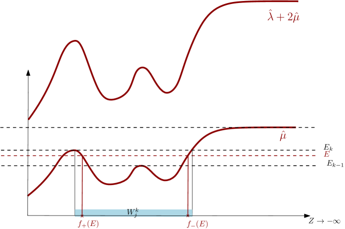
Fig. 1: Illustration of a well of order $k$ ($N_{k}=1$) and associated $f_{\pm}$.

4.2 Reconstruction

We note that Assumption 2.1 is needed here. We summarize the procedure:

• We start by constructing the half well, $\widetilde{W}^{1}$, that is connected to the boundary between $E_{0}$ and $E_{1}$.

• Inductively, we assume that we have already recovered the profile under $E_{k-1}$. First we reconstruct the half well, $\widetilde{W}^{k}$, of order $k$ between $E_{k-1}$ and $E_{k}$.

• We note that $\widetilde{W}^{k}$ must be a continuation of the half well $\widetilde{W}^{k-1}$, or be joined with some well, $W^{k-1}_{j}$, indexed by $j$ of order $k-1$.

• Then we reconstruct a monotonic piece. This can be done as in Section 2.3 using $\widetilde{S}_{0}^{k}$ only.

• Secondly, we consider the reconstruction of a full well, $W^{k}_{j}$, separated from the boundary, of order $k$:

Case I. The well $W^{k}_{j}$ might be a new well. Then we define the functions $f_{\pm}:\ [E_{k-1},E_{k}[\to I$ so that $W^{j}_{k}(E)=[f_{-}(E),f_{+}(E)]$ for any $E\in[E_{k-1},E_{k}[$.

Case II. The well $W^{k}_{j}$ might also be joining two wells of order $k-1$, or extending a single well of order $k-1$. Note that the profile under $E_{k-1}$ has already been recovered. The smooth joining of two wells can be carried out under Assumption 4.2. We consider now functions $f_{-}(E)$ and $f_{+}(E)$ for $E\in[E_{k-1},E_{k}]$ such that $W^{k}_{j}$ is the union of three connected intervals,

$$W^{k}_{j}(E_{k})=[f_{-}(E_{k}),f_{-}(E_{k-1})[\,\cup\,[f_{-}(E_{k-1}),f_{+}(E_{k-1})]\,\cup\,]f_{+}(E_{k-1}),f_{+}(E_{k})].$$

For an illustration, see Figure 1.

For either case, we define

(64) $$\Phi(E)=f_{+}^{\prime}(E)-f_{-}^{\prime}(E),\qquad\Psi(E)=\frac{1}{f_{+}^{\prime}(E)}-\frac{1}{f_{-}^{\prime}(E)}.$$

The recovery goes through explicit reconstruction of the entire profile following from the gluing procedure as outlined in [6, Section 5.4]. As in the case of the Love modes, the function $\Phi$ can be recovered from $S_{0}^{k,j}(E)$, on $]E_{k-1},E_{k}[$. From $S^{k,j}_{2}(E)$, we recover

(65) $$\mathcal{B}\Psi(E)=\int_{E_{k-1}}^{E}\left((7E-6u)\Psi^{\prime}(u)-2\left(\frac{E}{u}-1\right)\Psi(u)\right)\frac{\mathrm{d}u}{\sqrt{u(E-u)}}\\ -\int_{E_{k-1}}^{E}\left(36\Psi^{\prime}(u)-24\sigma\frac{1}{u}\Psi(u)\right)\arctan\sqrt{\frac{{E-u}}{u}}\mathrm{d}u,$$

$E_{k-1}<E<E_{k}$, where $\sigma=8\nu(1-2\nu)$. This is established in Appendix A.1. We introduce operator $T$ according to

(66) $$Tg(E)=\int_{E_{k-1}}^{E}\frac{g(u)}{\sqrt{E-u}}\mathrm{d}u.$$

In Appendix A.2, upon setting $E=z^{2}$, we prove that

(67) $$\frac{2}{\pi}z^{2}\frac{\mathrm{d}^{3}}{\mathrm{d}z^{3}}(T\circ\mathcal{B}\Psi)(z^{2})=16z^{6}\Psi^{\prime\prime\prime}(z^{2})-192z^{4}\Psi^{\prime\prime}(z^{2})+96(2-\sigma)z^{2}\Psi^{\prime}(z^{2})-96\sigma\Psi(z^{2}).$$

That is, we end up with a third-order inhomogeneous ordinary differential equation for $\Psi(z^{2})$ nonsingular on the interval $[\sqrt{E_{k-1}},\sqrt{E_{k}}[\,$. This equation needs to be supplemented with “initial” conditions:

For Case I, $\Psi(E_{k-1})$ and the asymptotic behaviors of $\Psi^{\prime}(E)$ and $\Psi^{\prime\prime}(E)$ for $E$ in a neighborhood of $E_{k-1}$ can be extracted from $T\circ\mathcal{B}\Psi(E)$ and its derivatives at $E_{k-1}$. Clearly, $\Psi(E_{k-1})=0$. Using the derivatives evaluated in Appendix A.2 and

(68) $$\Psi(E_{k-1})=0,\quad\lim_{E\downarrow E_{k-1}}\sqrt{E-E_{k-1}}\Psi^{\prime}(E)=\sqrt{2\hat{\mu}^{\prime\prime}(Z_{k-1})},$$

we obtain, for $E>E_{k-1}$ close to $E_{k-1}$,

(69) $$\lim_{E\downarrow E_{k-1}}\left(4E\Psi^{\prime}(E)-\frac{2}{\pi}\frac{\mathrm{d}}{\mathrm{d}z}(T\circ\mathcal{B}\Psi)(z^{2})\right)=0$$

yielding the asymptotic behavior of $\Psi^{\prime}(E)$, and

(70) $$\lim_{E\downarrow E_{k-1}}\left(-108E^{1/2}\Psi^{\prime}(E)+8E^{3/2}\Psi^{\prime\prime}(E)-\frac{\mathrm{d}^{2}}{\mathrm{d}z^{2}}(T\circ\mathcal{B}\Psi)(z^{2})\right)=0$$

yielding the asymptotic behavior of $\Psi^{\prime\prime}(E)$. With these, the solution to the third-order inhomogeneous ordinary differential equation is unique.

For Case II, $\Psi(E_{k-1})$, $\Psi^{\prime}(E_{k-1})$ and $\Psi^{\prime\prime}(E_{k-1})$ are all nonsingular. That is, if $E_{k-1}$ is a local maximum, $\Psi$ and all its derivatives are smooth from above and below, and therefore they can be recovered from the reconstruction on $J_{k-1}$ through one-sided limits. We note that in case $E_{k-1}$ is a local maximum in the middle of two wells in $J_{k-1}$ the two different $\Psi$s for each well are not smooth below $E_{k-1}$, but it does not matter as in $J_{k}$ (above $E_{k-1}$) we use $f_{\pm}$ from the monotonically increasing slopes continued from $J_{k-1}$. Thus the solution to the third-order inhomogeneous ordinary differential equation is also unique.

With the recovery of $\Phi$ and $\Psi$ we can recover $f_{\pm}$ and then $\hat{\mu}$ as in the case of Love modes, again, subject to a gluing procedure.

Appendix A Recovery of $\Psi$

A.1 Proof of (65)

We start with the expressions for $J(E)$, $K(E)$ and $L(E)$ in Subsection 3.3. We apply a change of variable of integration and obtain,

$$J(E)= \int_{E_{k-1}}^{E}\left(E\frac{\mathrm{d}}{\mathrm{d}u}\left(\frac{1}{f_{+}^{\prime}(u)}-\frac{1}{f_{-}^{\prime}(u)}\right)-2\left(\frac{E}{u}-1\right)\left(\frac{1}{f_{+}^{\prime}(u)}-\frac{1}{f_{-}^{\prime}(u)}\right)\right)\frac{\mathrm{d}u}{\sqrt{u(E-u)}}+J_{k-1}(E),$$

$$K(E)= \int_{E_{k-1}}^{E}\frac{\mathrm{d}}{\mathrm{d}u}\left(\frac{1}{f_{+}^{\prime}(u)}-\frac{1}{f_{-}^{\prime}(u)}\right)\frac{\mathrm{d}u}{\sqrt{u(E-u)}}+K_{k-1}(E),$$

$$L(E)= \int_{E_{k-1}}^{E}\frac{u}{E}\left(\frac{3}{2}\frac{\mathrm{d}}{\mathrm{d}u}\left(\frac{1}{f_{+}^{\prime}(u)}-\frac{1}{f_{-}^{\prime}(u)}\right)-4\left(\frac{\hat{\lambda}(f_{+}(u))}{(\hat{\lambda}(f_{+}(u))+u)^{2}}\frac{1}{f_{+}^{\prime}(u)}-\frac{\hat{\lambda}(f_{-}(u))}{(\hat{\lambda}(f_{-}(u))+u)^{2}}\frac{1}{f_{-}^{\prime}(u)}\right)\right)$$

$$\qquad\quad\frac{\mathrm{d}u}{\sqrt{u(E-u)}}+L_{k-1}(E).$$

For Case I (cf. Subsection 4.2), $J_{k-1}(E)$, $K_{k-1}(E)$ and $L_{k-1}(E)$ vanish. For Case II, $J_{k-1}(E)$, $K_{k-1}(E)$ and $L_{k-1}(E)$ are related to the profile on $[f_{-}(E_{k-1}),f_{+}(E_{k-1})]$:

(71) $$J_{k-1}(E) = \int_{Z_{-}}^{Z_{+}}\left(E\hat{\mu}^{\prime\prime}(Z)-2\left(\frac{E}{\hat{\mu}(Z)}-1\right)(\hat{\mu}^{\prime}(Z))^{2}\right)\frac{\mathrm{d}Z}{\sqrt{\hat{\mu}(Z)(E-\hat{\mu}(Z))}},$$

(72) $$K_{k-1}(E) = \int_{Z_{-}}^{Z_{+}}\hat{\mu}^{\prime\prime}\frac{\mathrm{d}Z}{\sqrt{\hat{\mu}(Z)(E-\hat{\mu}(Z))}},$$

(73) $$L_{k-1}(E) = \int_{Z_{-}}^{Z_{+}}\frac{\hat{\mu}}{E}\left(\frac{3}{2}\hat{\mu}^{\prime\prime}-\frac{4\hat{\lambda}(\hat{\mu}^{\prime})^{2}}{(\hat{\lambda}+\hat{\mu})^{2}}\right)\frac{\mathrm{d}Z}{\sqrt{\hat{\mu}(Z)(E-\hat{\mu}(Z))}},$$

where $Z_{-}=f_{-}(E_{k-1})$ and $Z_{+}=f_{+}(E_{k-1})$. These are already known.

We find that

$$K(E)-K_{k-1}(E)= \ 2\frac{\mathrm{d}}{\mathrm{d}E}\int_{E_{k-1}}^{E}(E-u)\Psi^{\prime}(u)\frac{\mathrm{d}u}{\sqrt{u(E-u)}},$$

$$L(E)-L_{k-1}(E)= \ 3\frac{\mathrm{d}}{\mathrm{d}E}\int_{E_{k-1}}^{E}\left(\Psi^{\prime}(u)-2\sigma\frac{1}{u}\Psi(u)\right)\arctan\sqrt{\frac{{E-u}}{u}}\mathrm{d}u.$$

Following [4, Lemma 13.1], we introduce an operator $\mathcal{B}$ defined by

(74) $$\mathcal{B}\Psi(E)=\int_{E_{k-1}}^{E}\left((7E-6u)\Psi^{\prime}(u)-2\left(\frac{E}{u}-1\right)\Psi(u)\right)\frac{\mathrm{d}u}{\sqrt{u(E-u)}}\\ -\int_{E_{k-1}}^{E}\left(36\Psi^{\prime}(u)-24\sigma\frac{1}{u}\Psi(u)\right)\arctan\sqrt{\frac{{E-u}}{u}}\mathrm{d}u.$$

Using (54), we have established that the derivative of $\mathcal{B}\Psi$ can be recovered from $S_{2}^{k,j}$. Then $\mathcal{B}\Psi$ itself can be recovered using $\mathcal{B}\Psi(E_{k-1})=\pi\sqrt{2\hat{\mu}^{\prime\prime}(Z_{k-1})E_{k-1}}$.

A.2 Proof of (67)

We have

(75) $$(T\circ\mathcal{B}\Psi)(E)=I_{1}(E)+I_{2}(E)+I_{3}(E)+\sigma I_{4}(E),$$

where

(76) $$I_{1}(E) = \int_{E_{k-1}}^{E}\frac{u}{\sqrt{E-u}}\int_{E_{k-1}}^{u}\left(7\Psi^{\prime}(v)-\frac{2}{v}\Psi(v)\right)\frac{1}{\sqrt{v}}\frac{1}{\sqrt{u-v}}\,\mathrm{d}v\mathrm{d}u,$$

(77) $$I_{2}(E) = \int_{E_{k-1}}^{E}\frac{1}{\sqrt{E-u}}\int_{E_{k-1}}^{u}\left(-6v\Psi^{\prime}(v)+2\Psi(v)\right)\frac{1}{\sqrt{v}}\frac{1}{\sqrt{u-v}}\,\mathrm{d}v\mathrm{d}u,$$

(78) $$I_{3}(E) = -36\int_{E_{k-1}}^{E}\frac{1}{\sqrt{E-u}}\int_{E_{k-1}}^{u}\arctan\sqrt{\frac{{u-v}}{v}}\Psi^{\prime}(v)\,\mathrm{d}v\mathrm{d}u,$$

(79) $$I_{4}(E) = 24\int_{E_{k-1}}^{E}\frac{1}{\sqrt{E-u}}\int_{E_{k-1}}^{u}\frac{1}{v}\arctan\sqrt{\frac{{u-v}}{v}}\Psi(v)\,\mathrm{d}v\mathrm{d}u.$$

Upon integration by parts, we obtain

$$I_{3}(E)= -36\int_{E_{k-1}}^{E}\frac{1}{u}\sqrt{E-u}\left(\int_{E_{k-1}}^{u}\sqrt{v}\Psi^{\prime}(v)\frac{\mathrm{d}v}{\sqrt{u-v}}\right)\mathrm{d}u$$

$$= -36E\int_{E_{k-1}}^{E}\frac{1}{u}\frac{1}{\sqrt{E-u}}\left(\int_{E_{k-1}}^{u}\sqrt{v}\Psi^{\prime}(v)\frac{\mathrm{d}v}{\sqrt{u-v}}\right)\mathrm{d}u$$

$$\qquad\qquad+36\int_{E_{k-1}}^{E}\frac{1}{\sqrt{E-u}}\left(\int_{E_{k-1}}^{u}\sqrt{v}\Psi^{\prime}(v)\frac{\mathrm{d}v}{\sqrt{u-v}}\right)\mathrm{d}u,$$

$$I_{4}(E)= 24\int_{E_{k-1}}^{E}\frac{1}{u}\sqrt{E-u}\left(\int_{E_{k-1}}^{u}\frac{1}{\sqrt{v}}\Psi(v)\frac{\mathrm{d}v}{\sqrt{u-v}}\right)\mathrm{d}u$$

$$= 24E\int_{E_{k-1}}^{E}\frac{1}{u}\frac{1}{\sqrt{E-u}}\left(\int_{E_{k-1}}^{u}\frac{1}{\sqrt{v}}\Psi(v)\frac{\mathrm{d}v}{\sqrt{u-v}}\right)\mathrm{d}u-24\int_{E_{k-1}}^{E}\frac{1}{\sqrt{E-u}}\left(\int_{E_{k-1}}^{u}\frac{1}{\sqrt{v}}\Psi(v)\frac{\mathrm{d}v}{\sqrt{u-v}}\right)\mathrm{d}u.$$

Now, we use some calculus

$$\int_{E_{k-1}}^{E}\frac{1}{\sqrt{E-u}}\left(\int_{E_{k-1}}^{u}g(v)\frac{\mathrm{d}v}{\sqrt{u-v}}\right)\mathrm{d}u = \pi\int_{E_{k-1}}^{E}g(v)\mathrm{d}v,$$

$$\int_{E_{k-1}}^{E}\frac{u}{\sqrt{E-u}}\left(\int_{E_{k-1}}^{u}g(v)\frac{\mathrm{d}v}{\sqrt{u-v}}\right)\mathrm{d}u = \frac{\pi}{2}\int_{E_{k-1}}^{E}(v+E)g(v)\mathrm{d}v,$$

$$\int_{E_{k-1}}^{E}\frac{1}{u}\frac{1}{\sqrt{E-u}}\left(\int_{E_{k-1}}^{u}g(v)\frac{\mathrm{d}v}{\sqrt{u-v}}\right)\mathrm{d}u = \pi\int_{E_{k-1}}^{E}\frac{1}{\sqrt{Ev}}g(v)\mathrm{d}v$$

and get

$$I_{1}(E) = \frac{\pi}{2}\int_{E_{k-1}}^{E}(v+E)\left(7\Psi^{\prime}(v)-\frac{2}{v}\Psi(v)\right)\frac{1}{\sqrt{v}}\mathrm{d}v,$$

$$I_{2}(E) = \pi\int_{E_{k-1}}^{E}\left(-6v\Psi^{\prime}(v)+2\Psi(v)\right)\frac{1}{\sqrt{v}}\mathrm{d}v,$$

$$I_{3}(E) = 36\pi\int_{E_{k-1}}^{E}\left(v-\sqrt{Ev}\right)\Psi^{\prime}(v)\frac{1}{\sqrt{v}}\mathrm{d}v,$$

$$I_{4}(E) = 24\pi\int_{E_{k-1}}^{E}\left(\frac{\sqrt{E}}{\sqrt{v}}-1\right)\Psi(v)\frac{1}{\sqrt{v}}\mathrm{d}v.$$

We insert $E=z^{2}$, when trivially

$$\frac{2}{\pi}I_{1}(z^{2}) = \int_{E_{k-1}}^{z^{2}}(v+z^{2})\left(7\Psi^{\prime}(v)-\frac{2}{v}\Psi(v)\right)\frac{1}{\sqrt{v}}\mathrm{d}v,$$

$$\frac{2}{\pi}I_{2}(z^{2}) = 2\int_{E_{k-1}}^{z^{2}}\left(-6v\Psi^{\prime}(v)+2\Psi(v)\right)\frac{1}{\sqrt{v}}\mathrm{d}v,$$

$$\frac{2}{\pi}I_{3}(z^{2}) = 72\int_{E_{k-1}}^{z^{2}}\left(\sqrt{v}-z\right)\Psi^{\prime}(v)\mathrm{d}v,$$

$$\frac{2}{\pi}I_{4}(z^{2}) = 48\int_{E_{k-1}}^{z^{2}}\left(\frac{z}{v}-\frac{1}{\sqrt{v}}\right)\Psi(v)\mathrm{d}v.$$

By tedious calculations, we then find that

$$\frac{2}{\pi}\frac{\mathrm{d}}{\mathrm{d}z}I_{1}(z^{2}) = 28z^{2}\Psi^{\prime}(z^{2})-8\Psi(z^{2})+\int_{E_{k-1}}^{z^{2}}2z\left(7\Psi^{\prime}(v)-\frac{2}{v}\Psi(v)\right)\frac{1}{\sqrt{v}}\mathrm{d}v,$$

$$\frac{2}{\pi}\frac{\mathrm{d}^{2}}{\mathrm{d}z^{2}}I_{1}(z^{2}) = 68z\Psi^{\prime}(z^{2})+56z^{3}\Psi^{\prime\prime}(z^{2})-8\frac{1}{z}\Psi(z^{2})+\int_{E_{k-1}}^{z^{2}}2\left(7\Psi^{\prime}(v)-\frac{2}{v}\Psi(v)\right)\frac{1}{\sqrt{v}}\mathrm{d}t,$$

$$\frac{2}{\pi}\frac{\mathrm{d}^{3}}{\mathrm{d}z^{3}}I_{1}(z^{2}) = 112z^{4}\Psi^{\prime\prime\prime}(z^{2})+304z^{2}\Psi^{\prime\prime}(z^{2})+80\Psi^{\prime}(z^{2})$$

and

$$\frac{2}{\pi}\frac{\mathrm{d}}{\mathrm{d}z}I_{2}(z^{2}) = -24z^{2}\Psi^{\prime}(z^{2})+8\Psi(z^{2}),$$

$$\frac{2}{\pi}\frac{\mathrm{d}^{2}}{\mathrm{d}z^{2}}I_{2}(z^{2}) = -48z^{3}\Psi^{\prime\prime}(z^{2})-32z\Psi^{\prime}(z^{2}),$$

$$\frac{2}{\pi}\frac{\mathrm{d}^{3}}{\mathrm{d}z^{3}}I_{2}(z^{2}) = -96z^{4}\Psi^{\prime\prime\prime}(z^{2})-208z^{2}\Psi^{\prime\prime}(z^{2})-32\Psi^{\prime}(z^{2})$$

and

$$\frac{2}{\pi}\frac{\mathrm{d}}{\mathrm{d}z}I_{3}(z^{2}) = -72\int_{E_{k-1}}^{z^{2}}\Psi^{\prime}(v)\mathrm{d}v,$$

$$\frac{2}{\pi}\frac{\mathrm{d}^{2}}{\mathrm{d}z^{2}}I_{3}(z^{2}) = -144z\Psi^{\prime}(z^{2}),$$

$$\frac{2}{\pi}\frac{\mathrm{d}^{3}}{\mathrm{d}z^{3}}I_{3}(z^{2}) = -288z^{2}\Psi^{\prime\prime}(z^{2})-144\Psi^{\prime}(z^{2})$$

and

$$\frac{2}{\pi}\frac{\mathrm{d}}{\mathrm{d}z}I_{4}(z^{2}) = 48\int_{E_{k-1}}^{z^{2}}\frac{1}{v}\Psi(v)\mathrm{d}v,$$

$$\frac{2}{\pi}\frac{\mathrm{d}^{2}}{\mathrm{d}z^{2}}I_{4}(z^{2}) = 96\frac{1}{z}\Psi(z^{2}),$$

$$\frac{2}{\pi}\frac{\mathrm{d}^{3}}{\mathrm{d}z^{3}}I_{4}(z^{2}) = 192\Psi^{\prime}(z^{2})-96\frac{1}{z^{2}}\Psi(z^{2}).$$

These identities lead us to (67).

References

- [1] M. Abramowitz and I.A. Stegun. Handbook of Mathematical Functions. Dover, New York, 2002.
- [2] M. Brocher, Empirical Relations between Elastic Wavespeeds and Density in the Earth’s Crust, Bull. Seism. Soc. Am. 95, (2005), pp.2081–2092.
- [3] Y. Colin de Verdière. Bohr-Sommerfeld Rules to All Orders. Ann. Henri Poincaré, 6:925–936, 2005.
- [4] Y. Colin de Verdière. A semi-classical inverse problem II: reconstruction of the potential. In Geometric aspects of analysis and mechanicss, volume 292, pages 97–119. Progr. Math., 2011.
- [5] M.V. de Hoop, A. Iantchenko, G. Nakamura, J. Zhai, Semiclassical analysis of elastic surface waves, arXiv:1709.06521.
- [6] M.V. de Hoop, A. Iantchenko, R. D. Van der Hilst, J. Zhai, Semiclassical inverse spectral problem for elastic Love surface waves in isotropic media, arXiv:1908.10529.
- [7] A. Derode, E. Larose, M. Tanter, J. de Rosny, A. Tourin, M. Campillo and M. Fink, Recovering the Green’s function form field-field correlations in an open scattering medium, J. Acoust. Soc. Am. 113, (2004), pp. 2973–2976.
- [8] M. Dimassi and J. Sjöstrand, Spectral asymptotics in the semiclassical limit, London Mathematical Society Lecture Notes Series 268, Cambridge University Press (1991).
- [9] B. Helffer and J. Sjöstrand, Analyse semi-classique de l’équation de Harper, II, Comportement semi-classique près d’un rationnel, Mém. Soc. Math. France, 40, 1990.
- [10] A. Martinez. An Introduction to Semiclassical and Microlocal Analysis. Springer, Berlin, 2002.
- [11] N. Shapiro and M. Campillo, Emergence of broadband Rayleigh waves from correlations of the ambient seismic noise, Geophys. Res. Lett. 31, (2004), L07614.
- [12] N. Shapiro, M. Campillo, L. Stehly and M. Ritzwoller, High resolution surface wave tomography from ambient seismic noise, Science 307, (2005), 1615.
- [13] B.L.N. Kennett and J.H. Woodhouse, On high-frequency spheroidal modes and structure of the upper mantle, Geophys. J.R. astr. Soc. 55, (1978), pp.333–350.
- [14] J.H. Woodhouse, Asymptotic results for elastodynamic propagator matrices in plane-stratified and spherically-stratified earth models, Geophys. J.R. astr. Soc. 54, (1978), pp.263–280.