Elimination of spectral blocking by ensuring rotation-free property of discretised pressure gradient within a spectral semi-implicit semi-Lagrangian global atmospheric model

Abstract

The widely-adopted discretisation of the horizontal pressure gradient term formulated by Simmons and Burridge (1981) for atmospheric models on $\sigma$-$p$ hybrid vertical coordinate is found to incur spectral blocking for rotational wind components at high vertical levels when used in a spectral semi-Lagrangian model run on a linear grid. A remedy to this issue is proposed and tested using a spectral semi-implicit semi-Lagrangian hydrostatic primitive equations model. The proposed method removes aliasing errors at high wavenumbers by ensuring that the rotation-free property of the pressure gradient term on isobaric surface, a feature possessed by the continuous system, is preserved in the discretised system, which highlights the significance of mimetic discretisation within the context of numerical weather prediction models.

This is the submitted version of the following article: Ujiie and Hotta (2019; QJRMS), which has been published in final form at https://doi.org/10.1002/qj.3636. This article may be used for non-commercial purposes in accordance with Wiley Terms and Conditions for Self-Archiving.

1 Introduction

“Spectral blocking” is a phenomenon often encountered in numerical time-marching solution of nonlinear partial differential equations that is characterised by a turn-up of power-spectra near the truncation limit (Boyd, 2001). On a map, spectral blocking often manifests itself as small-scale noises which, if left uncontrolled, can destabilise model integration. Spectral blocking is also undesirable because it means that the numerical solution in the high wavenumber range is dominated by noises rather than physically meaningful signals (e.g. Lander and Hoskins, 1997). It is therefore of prime importance to identify the cause of the spectral blocking and to take appropriate measures to eliminate or at least mitigate it. Note that, unlike its name may suggest, spectral blocking can occur with any discretisation method, not limited to the spectral method.

Spectral blocking has been recognised early in the history of climate and numerical weather prediction (NWP) model development when the primary source of nonlinearity was the quadratic Eulerian advection term, and various methods to counteract it have been proposed. For a finite-difference model, Arakawa (1966) devised a Jacobian (advection) discretisation that ensures energy and enstrophy conservation, whereby preventing small-scale noises to grow indefinitely; for a spectral model, Orszag (1970) introduced quadratic grid truncation rule which eliminates aliasing from quadratic terms by throwing away the highest one-third of the spectra that can be represented with a given model grid. Following Orszag (1970), all spectral atmospheric models with Eulerian advection scheme adopted quadratic (or higher-order) grid truncation. Later, when semi-Lagrangian advection schemes (Robert, 1981; Ritchie, 1988) were introduced that do not explicitly treat the quadratic advection terms, these schemes were shown to be able to control aliasing even with linear grid truncation (Côté and Staniforth, 1988), which led many operational spectral semi-Lagrangian models, including European Centre for Medium-range Weather Forecasts (ECMWF)’s Integrated Forecasting System (IFS), National Centers for Environmental Prediction (NCEP)’s Global Forecasting System (GFS) and Japan Meteorological Agency (JMA)’s Global Spectral Model (GSM), to adopt linear grids (Hortal, 2002; Katayama et al., 2005; Sela, 2010). We remark here that the advection terms, while being the dominant ones, are only one of the many sources of nonlinearity in the atmospheric governing equations (the others include physical parameterisation, pressure gradient terms in the momentum equations, and the adiabatic heating term in the thermodynamic equation, just to name a few), so that the absence of advection terms in the semi-Lagrangian schemes does not necessarily guarantee absence of the aliasing problem.

In JMA-GSM, the presence of spectral blocking became increasingly apparent as the resolution increased. As an example, Left panels of Figure 1 show the rotational and divergent component of the kinetic energy spectra computed for GSM’s two-day forecast initialised at a particular date. Spectral blocking appears for the rotational component (thick lines) and curiously, it is stronger in the upper levels (Figure 1a) than in the lower levels (Figure 1b). After an extensive investigation at JMA aiming at understanding this issue, the pressure gradient discretisation in the vertical, formulated following Simmons and Burridge (1981, SB81, hereafter), was found to be primarily responsible for this spectral blocking.

In this note, we describe why the discretisation of the pressure gradient terms adopted in JMA-GSM following SB81 can produce spectral blocking in the rotational wind component, and show how this problem can be remedied. As we show later in this note, the key is to ensure that the vector calculus identity (that the curl of gradient of any scalar field is zero) is preserved in the discretised system, which highlights the importance of “mimetic discretisation” in the context of NWP and climate modelling.

The rest of this note is structured as follows. Section 2 reviews the discretisation of the pressure gradient terms on $\sigma$-$p$ hybrid coordinate given in SB81 and discusses how, depending on specific implementation, it may cause spectral blocking when combined with a spectral horizontal discretisation. Section 3 proposes a method to alleviate this issue. Sections 4 and 5 describe the setup of idealised and realistic experiments along with the results. Section 6 concludes the note with discussions on its implication for future development of dynamical cores.

The pressure gradient formulation adopted in JMA-GSM is typical of many spectral semi-implicit semi-Lagrangian (SISL) atmospheric models, including ECMWF-IFS (ECMWF, 2018), SISL version of National Center for Atmospheric Research (NCAR) Community Atmospheric Model (CAM) (Williamson and Olson, 1994), Météo France’s ALADIN regional model (Bénard et al., 2010), and NCEP-GFS (Sela, 2010). We thus anticipate that the solution we found can also be helpful to other models in resolving (if present) similar issues.

2 Pressure gradient discretisation on $\sigma$-$p$ hybrid vertical levels following SB81

On a terrain-following $\sigma$-$p$ hybrid vertical coordinate parameterised by $\eta\in[0,1]$ where $\eta$ is defined such that the pressure $p$ can be expressed as $p=A(\eta)+B(\eta)p_{s}$ in terms of surface pressure $p_{s}$ and some functions $A$ and $B$, the hydrostatic pressure gradient $\mathbf{F}_{\mathrm{pgrad}}=-\nabla_{p}\Phi$ on the right-hand side (RHS) of the momentum equations is expressed as

$$\mathbf{F}_{\mathrm{pgrad}}= -\nabla_{p}\Phi=-\nabla_{\eta}\Phi-R_{d}T_{v}\nabla_{\eta}\ln{p},\quad\mbox{with}$$ (1)

$$\Phi =\Phi_{s}+\int_{p}^{p_{s}}R_{d}T_{v}d\ln{p},$$ (2)

where $\Phi,T_{v}$ and $R_{d}$ are, respectively, the geopotential, virtual temperature, and the gas constant for dry atmosphere. The subscript $s$ signifies values at the surface, and the subscripts $p$ and $\eta$ given to the gradient operator $\nabla$ signify that the derivative is taken along the isobaric and iso-$\eta$ surfaces, respectively. Note that the pressure gradient terms become rotation-free on upper atmosphere where the $\eta$-levels become isobaric ($B(\eta)=0$) because the first term on Equation 1 is rotation-free from vector calculus identity ($\nabla_{\eta}\times\nabla_{\eta}\equiv 0$) and the second term is identically zero for isobaric surfaces:

$$\nabla_{\eta}\times\mathbf{F}_{\mathrm{pgrad}}=\mathbf{0}\quad\mbox{for}\quad\eta\quad\mbox{such that}\quad B(\eta)=0.$$ (3)

SB81 derived a vertical discretisation on $\eta$ levels that conserves globally averaged angular momentum. Counting the levels from the surface ($k=1$) up to the model top ($k=k_{\mathrm{max}}$), the hydrostatic relation (Equation 2) is discretised as

$$\Phi_{k}=\Phi_{s}+\sum_{l=1}^{k-1}R_{d}T_{v,l}\ln\left(\frac{p_{l-1/2}}{p_{l+1/2}}\right)+\alpha_{k}R_{d}T_{v,k}$$ (4)

to give

$$-\nabla_{\eta}\Phi_{k}=-\nabla_{\eta}\Phi_{s}-\sum_{l=1}^{k-1}R_{d}\nabla_{\eta}\left[T_{v,l}\ln\left(\frac{p_{l-1/2}}{p_{l+1/2}}\right)\right]-\alpha_{k}R_{d}\nabla_{\eta}T_{v,k},$$ (5)

where the subscripts $k$ and $l$ denote discretised values at $k$-th and $l$-th full levels, the subscripts $l\pm 1/2$ denote the values at half levels, and $\alpha_{k}$ is defined as $\left[1-\frac{p_{k+1/2}}{\Delta p_{k}}\ln\left(\frac{p_{k-1/2}}{p_{k+1/2}}\right)\right]$ (for $k\neq k_{\mathrm{max}}$) where $\Delta p_{k}:=p_{k-1/2}-p_{k+1/2}$ and $\alpha_{k_{\mathrm{max}}}=\ln{2}$. Similarly the second term in Equation 1 at full levels is discretised as

$$-\left({R_{d}T_{v}}\nabla_{\eta}\ln{p}\right)_{k} =-\frac{R_{d}T_{v,k}}{\Delta p_{k}}\left[\ln\frac{p_{k-1/2}}{p_{k+1/2}}\nabla_{\eta}p_{k+1/2}+\alpha_{k}\nabla_{\eta}\Delta p_{k}\right].$$ (6)

The SB81 discretisation shown above is adopted by many $\eta$-coordinate models but how the pressure gradient terms are precisely computed varies depending on specific implementation of each model.

In spectral models, naive evaluation of Equation 6 may require a spectral transform of a three-dimensional variable $p$ (or $\ln{p}$) to compute its gradient, which is not economical since $\nabla_{\eta}p$ (or $\nabla_{\eta}\ln{p}$) is not used elsewhere in the model. SB81 suggested to economise computation by using the vertical coordinate definition

$$p_{k-1/2} =A_{k-1/2}+B_{k-1/2}p_{s}$$ (7)

to express the horizontal derivatives in Equation 6 in terms of $\nabla_{\eta}T_{v,k}$ and $\nabla_{\eta}p_{s}$ (or $\nabla_{\eta}\ln{p_{s}}$). In semi-Lagrangian models based on ‘$U$-$V$’ formulation (Ritchie, 1988; Temperton, 1991), we can further avoid spectral transform on another three-dimensional variable $\Phi$ by applying a similar strategy on Equation 5; symbolically, the pressure gradient terms are expressed as

$$\mathbf{F}_{\mathrm{pgrad},k} =-\nabla_{\eta}\Phi_{k}-\left({R_{d}T_{v}}\nabla_{\eta}\ln{p}\right)_{k}$$ (8)

$$\nabla_{\eta}\Phi_{k} =\nabla_{\eta}\Phi_{s}+\sum_{l=1}^{k}F_{l,k}(p_{s},T_{v})\nabla_{\eta}T_{v,l}+G_{k}(p_{s},T_{v})\nabla_{\eta}\ln{p_{s}}$$ (9)

$$\left({R_{d}T_{v}}\nabla_{\eta}\ln{p}\right)_{k} =\sum_{l=1}^{k}H_{l,k}(p_{s},T_{v})\nabla_{\eta}T_{v,l}+I_{k}(p_{s},T_{v})\nabla_{\eta}\ln{p_{s}}.$$ (10)

where the derivatives $\nabla_{\eta}\Phi_{s},\nabla_{\eta}T_{v,k}$ and $\nabla_{\eta}\ln{p_{s}}$ are evaluated spectrally. Examples of precise expressions can be found in, e.g., ECMWF (2018) and Sela (2010). This way, the number of variables to be represented spectrally is minimised, hence necessitating minimal numbers of grid-to-wave and wave-to-grid transforms per each time step.

JMA-GSM, before its May 2017 update (Yonehara et al., 2018), adopted a similar strategy but further simplified the expression by exploiting the fact that the second term on the RHS of Equation 5 and the second term on the RHS of Equation 6, if expanded, share common terms that, when combined, cancel each other. By cancelling them out, the expression for the pressure gradient terms reduces to

$$\begin{split}\mathbf{F}_{\mathrm{pgrad},k}=-\nabla_{\eta}\Phi_{s}-\sum_{l=1}^{k-1}R_{d}\ln\left(\frac{p_{l-1/2}}{p_{l+1/2}}\right)\nabla_{\eta}T_{v,l}\\ -\sum_{l=1}^{k-1}R_{d}T_{v,l}\left(\frac{B_{l-1/2}}{p_{l-1/2}}-\frac{B_{l+1/2}}{p_{l+1/2}}\right)\nabla_{\eta}p_{s}\\ -\alpha_{k}R_{d}\nabla_{\eta}T_{v,k}-R_{d}T_{v,k}\frac{B_{k-1/2}}{p_{k-1/2}}\nabla_{\eta}p_{s},\end{split}$$ (11)

where the derivatives $\nabla_{\eta}\Phi_{s},\nabla_{\eta}T_{v,k}$ and $\nabla_{\eta}p_{s}$ are evaluated spectrally. This pre-cancelled formulation avoids loss of accuracy due to cancellation of significant digits and should be particularly helpful over steep orography.

As we remarked at the beginning of this section, the pressure gradient terms on isobaric levels are rotation-free in the continuous system (Equation 3). The discrete analogue as computed from Equations 8-10 or Equation 11, however, does not preserve this property even though the horizontal spectral discretisation guarantees the rotation-free property of scalar gradients ($\nabla_{\eta}\times\nabla_{\eta}(\cdot)=\mathbf{0}$). Since the pressure gradient terms are nonlinear with respect to the model’s prognostic variables, the purely numerical noises in rotational component induced by the inability of the pressure gradient discretisation to preserve the rotation-free property contain high-wavenumber components beyond the truncation limit, which alias back onto the resolved high-wavenumber spectra of the solution which then can accumulate over time steps, eventually manifesting itself as spectral blocking.

Note that this problem does not show up in semi-implicit ‘$\zeta$-$D$’ models (Hoskins and Simmons, 1975) since, in ‘$\zeta$-$D$’ formulation, the pressure gradient terms only appear in the divergence equation in the form of a Laplacian. Nonlinear aliasing does occur for the divergent component but it is well controlled by the selective high-wavenumber damping inherent in the semi-implicit Helmholtz solver.

3 Modified pressure gradient discretisation that alleviates spectral blocking

As we described in Section 2, the failure of the pressure gradient discretisation to preserve its rotation-free property on isobaric levels can result in nonlinear aliasing. This finding is not new, and Wedi et al. (2013) and Wedi (2014) reported that a symptom similar to ours depicted in Figure 1 was also found in ECMWF-IFS; they identified the rotational component of the pressure gradient terms as the primary source of aliasing, and further proposed two solutions to this issue, one being to apply a “de-aliasing” filter that effectively removes the upper one-third of the spectra of rotational component of the pressure gradient terms, and the other being to adopt a higher order grid truncation.

Here we propose an alternative solution. The rotation-free property on iso-baric levels (Equation 3) can be assured if we first compute the full-level geopotential $\Phi_{k}$ with Equation 4 in grid space and then evaluate its gradient $\nabla_{\eta}\Phi_{k}$ by spectral transform, and finally combine it with the rest of the pressure gradient (Equation 6) with $\nabla_{\eta}p_{k+1/2}$ and $\nabla_{\eta}\Delta p_{k}$ expressed in terms of $\nabla_{\eta}\ln{p_{s}}$ using Equation 7. This way, the absence of rotation on isobaric levels is automatically assured since the spectral evaluation of the horizontal gradient guarantees the identity $\nabla_{\eta}\times\nabla_{\eta}=\mathbf{0}$, and the second part coming from Equation 6 is identically zero on isobaric levels.

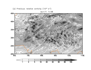
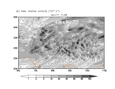
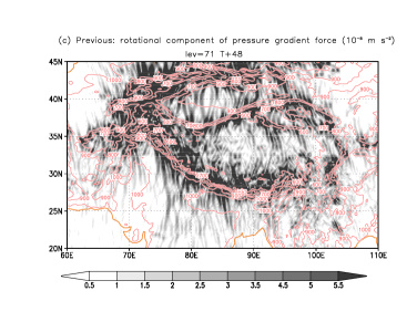
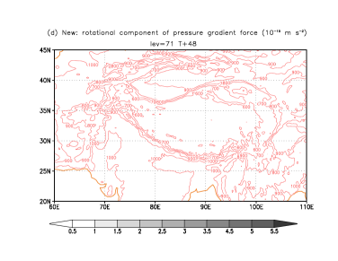
Figure 2: Maps, plotted for the Himalayas region, of (a,b) vorticity (units: $10^{-6}\mathrm{s}^{-1}$) and (c,d) the curl of pressure gradient (units: $10^{-5}\mathrm{ms}^{-2}$ in (c), $10^{-15}\mathrm{ms}^{-2}$ in (d)), both at 71st model level ($\sim$ 40 hPa), from 48-hour forecasts produced by JMA-GSM with (a,c) previous and (b,d) new pressure gradient discretisation schemes. In (a,b) the positive and negative contours are drawn, respectively, with solid and dashed lines, and the shades indicate the strength of vorticity. In (c,d) the curl of pressure gradient is plotted with shades, superpose on contours in lighter colours that show the surface pressure (units: hPa). Note that the scale of shades in (d) is $10^{-10}$ times smaller than in (c) to accentuate the small values. Shown are the results for the same case as in Figure 1.

Compared to the de-aliasing filter approach, the proposed method has the advantage of not introducing ad hoc correction nor tunable parameters. Higher order grid approach can account for nonlinear aliasing not only from pressure gradient but from any nonlinear terms; we remark nevertheless that it does not completely eliminate small-scale aliasing noises in rotational component of the pressure gradient (as we verified by running GSM with quadratic Tq639 grid and then plotting a map similar to Figure 2c, not shown) although they do not result in spectral blocking (i.e., turn-up of power spectra near the high-wavenumber end) since the filtering effect inherent in high order truncation prevents their accumulation over time steps. The higher order grid approach has another advantage of being much more cost effective than the regular linear grid truncation, particularly at very high resolutions, while allowing more accurate representation of small-scale variances (Malardel et al., 2016). The higher order grid approach and the proposed method are not mutually exclusive and can be used altogether.

The impact of adopting this alternative discretisation on spectral blocking is significant, as we can confirm by comparing the right and left panels of Figure 1. The spectral blocking observed with the previous discretisation (Equation 11) for the rotational component at an upper level (81st out of 100 levels, $\sim 11$ hPa; at this level, the iso-$\eta$ surface is isobaric) completely disappears with the proposed discretisation (Figure 1b). The blocking remains at the lower level (51st, $\sim 180$ hPa) where the iso-$\eta$ surface is close to but not completely parallel to the isobars, but to a much diminished degree (Figure 1d). The impact is also visible on a map as shown in Figure 2: with the previous discretisation, the vorticity at the 71st level ($\sim 40$ hPa) plotted over the Himalayas exhibited small-scale noisy patterns particularly along steep orography (Figure 2a); in contrast, with the proposed discretisation, the vorticity plot is much less noisy (Figure 2b). Similarly, the rotation (curl) of the pressure gradient computed with the previous discretisation exhibits small-scale noises (Figure 2c) but they disappear (to machine precision) by the proposed discretisation (Figure 2d).

The proposed method is very effective in reducing spectral blocking as shown above, but this benefit comes at the expense of additional computational and communication cost associated with one extra spectral transform for three-dimensional variable ($\Phi$). In the case of JMA-GSM, the increase of total execution time due to this additional transform was found to be relatively small, partly because $\Phi$ can be transformed together with $T_{v}$ so that the number of calls to MPI routines was not increased.

Another potential disadvantage of the proposed approach is the loss of pre-cancellation of compensating components in $\nabla_{\eta}\Phi$ and $R_{d}T_{v}\nabla_{\eta}\ln{p}$ exploited in the previous formulation of JMA-GSM (Equation 11), which may result in degradation in the model’s ability to maintain geostrophic balance, particularly in the presence of orography. This aspect is examined in next section using idealised test cases.

4 Idealised experiments

To assess how the proposed modification to pressure gradient discretisation affects the model’s ability to maintain balance, we performed two idealised test cases and compared the results obtained from the previous and proposed methods. The model we use is the dry dynamical core of JMA-GSM. As described in the previous section, it is a spectral SISL hydrostatic primitive equations (HPE) model discretised with spherical-harmonics-based spectral representation in the horizontal and finite differencing on 100 $\eta$-levels in the vertical extending from surface up to 0.01 hPa. The time step $\Delta t$ is taken as 720 s regardless of the horizontal resolution. Further details of the model can be found in Section 3.1 of Yukimoto et al. (2011) and Section 3.2.2 of JMA (2013).

4.1 Maintenance of resting atmosphere in the presence of orography

To highlight the impact of modifying pressure gradient discretisation only, we first conducted a maintenance test of resting atmosphere where, as in e.g. Klemp (2011), the model is initialised with a steady state in equilibrium with no wind. Ideally, the solution should stay at rest, but in the model the atmosphere may start to move since the discretised pressure gradient is not necessarily zero in the presence of orography.

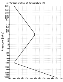
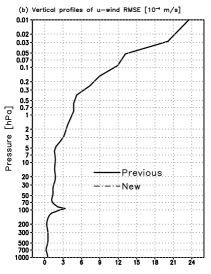
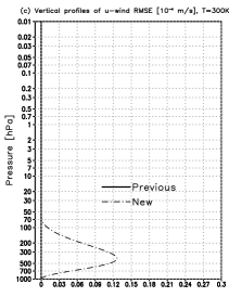
Figure 3: (a) Temperature profile prescribed in the resting-atmosphere maintenance test. (b) Profiles of the root-mean-square zonal winds horizontally averaged over the globe from 5-day forecasts (units: $10^{-4}\mathrm{m}{s}^{-1}$) produced using the previous and new pressure gradient discretisation schemes run at Tl319 horizontal resolution. (c) As in (b), but with the temperature profile replaced by a constant profile at 300 K. Note that, in (b), the two lines are indistinguishable since they collapsed onto a single line.

In this test, we prescribe a temperature profile as a function of pressure only that mimics the real atmosphere, as shown in Figure 3a. As the surface geopotential $\Phi_{s}$, we prescribe the two-dimensional bell defined by Equation 9 of Wedi and Smolarkiewicz (2009) with the radius of the Earth $a$ same as in the operation (no ‘small-planet’ setup) and the mountain half width $L_{\lambda}$ set to $0.12a$. The surface pressure $p_{s}$ is determined from the primitive equations so that the pressure gradient vanishes in the absence of winds.

The test is performed using JMA-GSM with the horizontal resolution of Tl319. The errors, measured as the square root of the horizontal average of the squared zonal wind from 5-day forecast, are shown for each vertical level in Figure 3b. The error from the previous method (thick line) and that from the proposed method (thin line) collapse onto a single profile, meaning that the model’s ability to maintain the state at rest is not harmed by using the proposed method. While the proposed scheme is as accurate as the original scheme for the realistic temperature profile, the original scheme did result in much smaller errors when the temperature profile shown in Figure 3a was replaced by a contrived iso-thermal temperature profile at 300 K (Figure 3c). This, together with the results for a more realistic profile, indicate that the pre-cancellation of compensating components exploited in the previous scheme is only effective for idealised (unrealistic) situations.

4.2 Jablonowski-Williamson steady sate test

To further assess the impact of using the proposed pressured gradient discretisation, we then conducted the steady-state test proposed by Jablonowski and Williamson (2006) which we believe is more holistic in that not only pressure gradient terms but also other terms of the governing equations play a role. In this test case the model is initialised with an analytically defined steady-state solution and integrated up to 9 days, to examine to what extent the model is able to maintain this steady state. The steady state is baroclinically unstable, so that imbalances induced by discretisation error will amplify and become detectable.

The steady-state test is performed using JMA-GSM with three different horizontal resolutions of Tl63, Tl319 and Tl959 (which correspond to grid spacing of $\sim 300$ km, $\sim 60$ km and $\sim 20$ km at the Equator, respectively), all with the operational 100 vertical levels. The globally-averaged $l_{2}$-deviation of the zonal wind field $u$ from their zonal mean (Equation 14 of Jablonowski and Williamson (2006): the error associated with growth of baroclinic waves) was larger with the proposed method than with the previous method but only by about 20–30% for Tl319 and Tl959 resolutions (at Tl63 resolution, the errors were almost identical; figures omitted). The temporal degradation of the zonal mean zonal wind field (Equation 15 of Jablonowski and Williamson (2006): the error associated with geostrophic adjustment in the discrete system) quickly saturated by day 1 and stayed around $2.5\times 10^{-3}\mathrm{m}\mathrm{s}^{-1}$ for any resolution with both the proposed and previous methods (figures omitted; the error curves were very similar to the one shown in Figure 5 of Hotta and Ujiie (2018)).

The results from the two sets of idealised experiments all suggest that the new pressure gradient discretisation is as accurate as the previous one except in the contrived isothermal setup, motivating us to conduct full NWP experiments at quasi-operational setup that we describe below.

5 Cycled NWP experiment

The impact of the proposed pressure gradient discretisation upon forecast performance was assessed by conducting cycled NWP experiments following the standard practice at JMA. We conducted cycled NWP experiments for two distinct periods (SUMMER and WINTER) that each covers more than a month. The SUMMER experiment consists of 6-hourly data assimilation cycle that begins on July 10, 2015 at 00 UTC and ends on September 11, 2015 at 18 UTC, and extended forecasts up to 11 days that are launched daily only at 12 UTC from July 21, 2015 till August 31, 2015. Similarly, the WINTER experiment consists of data assimilation cycle that begins on December 10, 2014 at 00UTC and ends on February 11, 2015 at 18 UTC, and extended forecasts launched daily at 12 UTC from December 21, 2014 to January 31, 2015.

The update of pressure gradient discretisation only resulted in neutral impact in terms of all headline scores (figures omitted). The first-guess fit to observations (O-B departures) were also closely examined, with particular focus on stratosphere-sensitive instruments like radiances from AMSU-A and microwave sounders and GNSS radio-occultation, but no significant differences were detected (figures omitted). From these results we conclude that the new discretisation successfully reduces spectral blocking in vorticity without harming forecast performance.

6 Conclusions

The vertical discretisation of the pressure gradient terms adopted by JMA-GSM following Simmons and Burridge (1981), which is typical of many global spectral HPE models on $\eta$ hybrid coordinate, is found to incur spectral blocking in the rotational winds, particularly in the upper layers where the iso-$\eta$ levels are (close to) isobaric. This results from the inability of grid-space evaluation of geopotential gradient $\nabla_{\eta}\Phi$ to preserve its rotation-free property, which is easily fixed by spectral evaluation of the $\nabla_{\eta}\Phi$ term as we proposed in section 3. The proposed method was tested in both idealised and quasi-operational experiments and was found to significantly reduce the spectral blocking without harming forecast performance. The proposed scheme was incorporated into JMA’s operational deterministic forecasting system in its May 2017 update (Yonehara et al., 2018). The presence of spectral blocking in spectral SISL models on linear grid, and the importance of assuring rotation-free property on the discretised gradient operator, have both been well-recognised, but the connection between the two appears not to be well clarified in the literature. Since the pressure gradient discretisation that we described in Section 2 is quite generic, the solution that we described in Section 3 should be widely applicable to other spectral SISL models as well.

The finding documented in this note highlights the importance of preserving rotation-free property in the discretised gradient operators. This is not a new discovery, and has already been emphasised by Staniforth and Thuburn (2012) as one of the essential desiderata for future dynamical cores. This is a challenging task, especially for grid-based discretisation, but, promising progress has already been made, for example, by Thuburn et al. (2014) and Weller and Shahrokhi (2014).

An interesting and useful lesson that we draw from the presented results is that pressure gradient discretisation as a whole can bear rotational component even if the mimetic “rotation-free gradient” property $(\nabla\times\nabla=0)$ is satisfied operator-wise (as with spectral representation). Given the current trend of high-performance computing where growth of computing capacity relies increasingly on massive parallelism, spectral models are predicted to face serious scalability issue, and many centers, including JMA, are exploring transition to (or have already transitioned to) a grid-based model with better data locality (e.g., Hotta and Ujiie, 2018; Kühnlein et al., 2019). The lesson that we learned here will serve nicely as a guiding principle in deciding which discretisation to use out of many possibilities.

CONFLICT OF INTEREST

Authors declare no conflict of interest.

Figures

Figure 1: Kinetic energy spectra of 48-hour forecasts produced by JMA-GSM with (a,c) previous and (b,d) new pressure gradient discretisation schemes, for (a,b) an upper level (81st model level, $\sim$ 11 hPa) and (c,d) a middle level (51st model level, $\sim$ 180 hPa). On each panel, the rotational and divergent components are plotted, respectively, with thick and thin lines. Units are $\mathrm{m}^{2}\mathrm{s}^{-2}$. Note the log scale on both axes. The forecasts are initialised with JMA’s operational deterministic analysis valid at December 25, 2018, 12 UTC.

References

- Arakawa (1966) Arakawa, A. (1966) Computational design for long-term numerical integration of the equations of fluid motion: Two-dimensional incompressional flow. part i. Journal of Computational Physics, 1, 119–143.
- Bénard et al. (2010) Bénard, P., Vivoda, J., Masek, J., Smolíková, P., Yessad, K., Brozkova, R. and Geleyn, J.-F. (2010) Dynamical kernel of the Aladin-NH spectral limited-area model : Revised formulation and sensitivity experiments. Quarterly Journal of the Royal Meteorological Society, 136, 155–169.
- Boyd (2001) Boyd, J. P. (2001) Chebyshev and Fourier spectral methods. Dover Publications Inc., second revised edn.
- Côté and Staniforth (1988) Côté, J. and Staniforth, A. (1988) A two-time-level semi-lagrangian semi-implicit scheme for spectral models. Monthly Weather Review, 116, 2003–2012.
- ECMWF (2018) ECMWF (2018) Part iii: Dynamics and numerical procedures. IFS Documentation—Cy45r1, 1–31.
- Hortal (2002) Hortal, M. (2002) The development and testing of a new two-time-level semi-lagrangian scheme (SETTLS) in the ECMWF forecast model. Quarterly Journal of the Royal Meteorological Society, 128, 1671–1687.
- Hoskins and Simmons (1975) Hoskins, B. J. and Simmons, A. J. (1975) A multi-layer spectral model and the semi-implicit method. Quarterly Journal of the Royal Meteorological Society, 101, 637–655.
- Hotta and Ujiie (2018) Hotta, D. and Ujiie, M. (2018) A nestable, multigrid-friendly grid on a sphere for global spectral models based on Clenshaw–Curtis quadrature. Quarterly Journal of the Royal Meteorological Society, 144, 1382–1397.
- Jablonowski and Williamson (2006) Jablonowski, C. and Williamson, D. L. (2006) A baroclinic instability test case for atmospheric model dynamical cores. Quarterly Journal of the Royal Meteorological Society, 132, 2943–2975.
- JMA (2013) JMA (2013) Outline of the operational numerical weather prediction at the Japan Meteorological Agency (March 2013), Appendix to WMO Technical Progress Report on the Global Data-processing and Forecasting System (GDPFS) and Numerical Weather Prediction (NWP) Research. 188pp. URL: http://www.jma.go.jp/jma/jma-eng/jma-center/nwp/outline2013-nwp/index.htm.
- Katayama et al. (2005) Katayama, K., Yoshimura, H. and Matsumura, T. (2005) Operational implementation of a new semi-lagrangian global nwp model at jma. CAS/JSC WGNE Research Activity on Atmospheric and Oceanic Modelling, 6.5–6.6.
- Klemp (2011) Klemp, J. (2011) A terrain-following coordinate with smoothed coordinate surfaces. Monthly Weather Review, 139, 2163–2169.
- Kühnlein et al. (2019) Kühnlein, C., Deconinck, W., Klein, R., Malardel, S., Piotrowski, Z. P., Smolarkiewicz, P. K., Szmelter, J. and Wedi, N. P. (2019) Fvm 1.0: a nonhydrostatic finite-volume dynamical core for the ifs. Geoscientific Model Development, 12, 651–676.
- Lander and Hoskins (1997) Lander, J. and Hoskins, B. J. (1997) Believable scales and parameterizations in a spectral transform model. Monthly Weather Review, 125, 292–303.
- Malardel et al. (2016) Malardel, S., Wedi, N., Deconinck, W., Diamantakis, M., Kühnlein, C., Mozdzynski, G., Hamrud, M. and Smolarkiewicz, P. (2016) A new grid for the IFS. ECMWF Newsletter, 146, 23–28.
- Orszag (1970) Orszag, S. A. (1970) Transform method for the calculation of vector-coupled sums: Application to the spectral form of the vorticity equation. Journal of the Atmospheric Sciences, 27, 890–895.
- Ritchie (1988) Ritchie, H. (1988) Application of the semi-lagrangian method to a spectral model of the shallow water equations. Monthly Weather Review, 116, 1587–1598.
- Robert (1981) Robert, A. (1981) A stable numerical integration scheme for the primitive meteorological equations. Atmosphere and Ocean, 19, 35–46.
- Sela (2010) Sela, J. (2010) The derivation of the sigma pressure hybrid coordinate semi-Lagrangian model equations for the GFS. NCEP Office Note, No. 462, 31pp.
- Simmons and Burridge (1981) Simmons, A. J. and Burridge, D. M. (1981) An energy and angular-momentum conserving vertical finite-difference scheme and hybrid vertical coordinates. Monthly Weather Review, 109, 758–766.
- Staniforth and Thuburn (2012) Staniforth, A. and Thuburn, J. (2012) Horizontal grids for global weather and climate prediction models: a review. Quarterly Journal of the Royal Meteorological Society, 138, 1–26.
- Temperton (1991) Temperton, C. (1991) On scalar and vector transform methods for global spectral models. Monthly Weather Review, 119, 1303–1307.
- Thuburn et al. (2014) Thuburn, J., Cotter, C. and Dubos, T. (2014) A mimetic, semi-implicit, forward-in-time, finite volume shallow water model: Comparison of hexagonal–icosahedral and cubed sphere grids. Geoscientific Model Development, 7, 909–929.
- Wedi (2014) Wedi, N. P. (2014) Increasing horizontal resolution in numerical weather prediction and climate simulations: illusion or panacea? Philosophical Transactions of the Royal Society A: Mathematical, Physical and Engineering Sciences, 372, 20130289.
- Wedi et al. (2013) Wedi, N. P., Hamrud, M. and Mozdzynski, G. (2013) The ecmwf model: progress and challenges. Proceedings of ECMWF Annual Seminar 2013: Recent developments in numerical methods for atmosphere and ocean modelling., 1–14.
- Wedi and Smolarkiewicz (2009) Wedi, N. P. and Smolarkiewicz, P. K. (2009) A framework for testing global non-hydrostatic models. Quarterly Journal of the Royal Meteorological Society, 135, 469–484.
- Weller and Shahrokhi (2014) Weller, H. and Shahrokhi, A. (2014) Curl-free pressure gradients over orography in a solution of the fully compressible euler equations with implicit treatment of acoustic and gravity waves. Monthly Weather Review, 142, 4439–4457.
- Williamson and Olson (1994) Williamson, D. L. and Olson, J. G. (1994) Climate simulations with a semi-lagrangian version of the ncar community climate model. 122, 1594–1610.
- Yonehara et al. (2018) Yonehara, H., Sekiguchi, R., Kanehama, T., Saitou, K., Kinami, T., Shimokobe, A., Hotta, D., R.Nagasawa, Sato, H., Ujiie, M., Kadowaki, T., Yabu, S., Yamada, K., Nakagawa, M. and Tokuhiro, T. (2018) Upgrade of JMA’s operational global NWP system. CAS/JSC WGNE Research Activity on Atmospheric and Oceanic Modelling, 48, 6.15–6.16.
- Yukimoto et al. (2011) Yukimoto, S., Yoshimura, H., Hosaka, M., Sakami, T., Tsujino, H., Hirabara, M., Tanaka, T., Deushi, M., Obata, A., Nakano, H., Adachi, Y., Shindo, E., Yabu, S., Ose, T. and Kitoh, A. (2011) Meteorological Research Institute-Earth System Model Version 1 (MRI-ESM1)– Model Description–. Technical Report of the Meteorological Research Institute, 64, 1–96.