Momentum distribution of the electron pair from the charged lepton flavor violating process $\mu^{-}e^{-}\to e^{-}e^{-}$ in muonic atoms with a polarized muon

Abstract

The $\mu^{-}e^{-}\to e^{-}e^{-}$ process in a muonic atom is one of the promising probes to study the charged lepton flavor violation (CLFV). We have investigated the angular distribution of electrons from the polarized muon of the atomic bound state. The parity violating asymmetric distribution of electrons is analyzed by using lepton wave functions under the Coulomb interaction of a finite nuclear charge distribution. It is found that the asymmetry parameters of electrons are very sensitive to the chiral structure of the CLFV interaction and the contact/photonic interaction. Therefore, together with the atomic number dependence of the decay rate studied in our previous work, the angular distribution of electrons from a polarized muon should be a very useful tool to constrain the model beyond the standard model.

I Introduction

The charged lepton flavor violation (CLFV) is an excellent probe of new physics beyond the standard model (SM) Calibbi2017 since it is highly suppressed in the SM. The best experimental constraints of the CLFV are obtained from exotic decays of muons, e.g., $Br\left(\mu^{+}\to e^{+}\gamma\right)<4.2\times 10^{-13}$ Baldini2016 , $Br\left(\mu^{+}\to e^{+}e^{+}e^{-}\right)<1.0\times 10^{-12}$ Bellgardt1988 , and $Br\left(\mu^{-}\textrm{Au}\to e^{-}\textrm{Au}\right)<7\times 10^{-13}$ Bertl2006 . Next-generation experiments are planned to discover CLFV Baldini2013 ; Blondel2013 ; COMET2018 ; Bartoszek2015 ; Nguyen2015 .

The $\mu^{-}e^{-}\to e^{-}e^{-}$ transition in a muonic atom was proposed as a new process to search for the CLFV in Ref. Koike2010 . The $\mu^{-}e^{-}\to e^{-}e^{-}$ process has interesting features complementary to the other CLFV searches. One of its important properties is the clear signal of the process; the total energy of two emitted electrons is equal to $m_{\mu}-B_{\mu}+m_{e}-B_{e}$, where $B_{\ell}$ is the binding energy of the lepton $\ell$ in an atomic orbit. A discussion to search for the $\mu^{-}e^{-}\to e^{-}e^{-}$ process is ongoing in the COMET Phase-I experiment at J-PARC COMET2018 .

In our recent work Uesaka2016 ; Uesaka2018 , careful calculations were made for the transition rate of the $\mu^{-}e^{-}\to e^{-}e^{-}$, which included the calculation of wave functions for the bound leptons in the initial state and the emitted electrons in the final state using a Dirac equation with a realistic charge distribution of nuclei. In calculating the rate of the $\mu^{-}e^{-}\to e^{-}e^{-}$ process, it is essential to take into account the relativistic effects for the bound leptons and the distortion effects for the emitted electrons with the finite charge distribution.

The effective Lagrangian of the CLFV process $\mu^{-}e^{-}\to e^{-}e^{-}$ is given as

$$\mathcal{L}_{CLFV}= \mathcal{L}_{\mathrm{photo}}+\mathcal{L}_{\mathrm{contact}},$$ (1)

$$\mathcal{L}_{\mathrm{photo}}= -\frac{4G_{F}}{\sqrt{2}}m_{\mu}\left[A_{R}\overline{e_{L}}\sigma^{\mu\nu}\mu_{R}+A_{L}\overline{e_{R}}\sigma^{\mu\nu}\mu_{L}\right]F_{\mu\nu}+[\mathrm{H.c.}],$$ (2)

$$\mathcal{L}_{\mathrm{contact}}= -\frac{4G_{F}}{\sqrt{2}}[g_{1}(\overline{e_{L}}\mu_{R})(\overline{e_{L}}e_{R})+g_{2}(\overline{e_{R}}\mu_{L})(\overline{e_{R}}e_{L})$$

$$+g_{3}(\overline{e_{R}}\gamma_{\mu}\mu_{R})(\overline{e_{R}}\gamma^{\mu}e_{R})+g_{4}(\overline{e_{L}}\gamma_{\mu}\mu_{L})(\overline{e_{L}}\gamma^{\mu}e_{L})$$

$$+g_{5}(\overline{e_{R}}\gamma_{\mu}\mu_{R})(\overline{e_{L}}\gamma^{\mu}e_{L})+g_{6}(\overline{e_{L}}\gamma_{\mu}\mu_{L})(\overline{e_{R}}\gamma^{\mu}e_{R})]+[\mathrm{H.c.}],$$ (3)

where $G_{F}=1.166\times 10^{-5}$GeV^-2 is the Fermi coupling constant, and $A_{L/R}$ and $g_{j}$ ($j=1,\cdots,6$) are the dimensionless coupling constants. The left- and right-handed projections are given as $P_{L/R}=(1\mp\gamma_{5})/2$, respectively. The $\mathcal{L}_{\mathrm{contact}}$ represents short range interaction and the $\mathcal{L}_{\mathrm{photo}}$ generates the one-photon-exchange process together with the ordinary electromagnetic interaction,

$$\mathcal{L}_{em}=-q_{e}\overline{e}\gamma^{\lambda}eA_{\lambda},$$ (4)

where $q_{e}=-e$ is a charge of an electron.

There are several clear differences on the interaction type. For example, the atomic number ($Z$) dependence of the transition rate is clearly different between photonic and contact interaction, though it was shown that it is proportional to $(Z-1)^{3}$ in both cases with the simple estimation given in Ref. Koike2010 . The cubic power of the atomic number arises from the wave functions of the initial bound states. However, we showed in our previous works Uesaka2016 ; Uesaka2018 that the $Z$ dependence is stronger and weaker than $(Z-1)^{3}$ for the contact and photonic interaction, respectively, by taking into account appropriate wave functions and a photon propagator for photonic interaction. As another example, in Ref. Uesaka2018 it was shown that the energy-angular distribution of emitted electrons is sensitive to the interaction type. With these facts, we can find which interaction is dominant.

However, the above observables do not depend on the chiral structure. The chiral structure of the CLFV interaction is an important key to search for the new physics. For example, it is well known that SU(5) and SO(10) supersymmetric grand unified theory gives different chiral structures in the CLFV interaction. To observe it in $\mu\to e\gamma$ and $\mu\to eee$, to make use of the muon polarization has been discussed in Refs. Kuno1996 ; Okada2000 . In this paper, we focus on the $\mu^{-}e^{-}\to e^{-}e^{-}$ search with a muon polarized in a muonic atom to extract the chiral property of the CLFV interaction. We start from our previous formulation of the $\mu^{-}e^{-}\to e^{-}e^{-}$ Uesaka2016 ; Uesaka2018 and then we extended the formalism to describe the electron asymmetry for the decay of a polarized muon in an atom. To determine the chiral structure of the CLFV interaction including parity violation, we investigate how the anisotropy in an electron momentum distribution depends on it.

In addition to the parity violating signal, we also analyze motion-reversal-odd observables. Even if the interaction Lagrangian includes no $CP$ violating terms, the final state interaction and other causes are known to induce the spurious $CP$ violation in observables. Therefore the estimation of the contribution for the spurious $CP$ violation is essential to measure the $CP$ violation of the CLFV interaction via the $\mu^{-}e^{-}\to e^{-}e^{-}$ process in the future.

In Sec. II, we formulate the $\mu^{-}e^{-}\to e^{-}e^{-}$ process in a muonic atom with a polarized bound muon. After we present the analytic formula for the plane wave approximation to understand the mechanism of electron asymmetry, we study the formula including the distortion of emitted electrons. In Sec. III, the results of numerical calculation are given and the possibilities to identify the structure of the CLFV operator are discussed. Finally, in Sec. IV, we summarize our analyses.

II Formulation

The $\mu^{-}e^{-}\to e^{-}e^{-}$ decay of the muonic atom is described in the independent particle model of a muonic atom. The transition amplitude $M$ of $\mu^{-}(1s,s_{\mu})+e^{-}(1s,s_{e})\to e^{-}(\bm{p}_{1},s_{1})+e^{-}(\bm{p}_{2},s_{2})$ is given as

$$2\pi i\delta(E_{1}+E_{2}-E_{tot})M(\bm{p}_{1},s_{1},\bm{p}_{2},s_{2};s_{\mu},s_{e})= \braket{e^{s_{1}}_{\bm{p}_{1}}e^{s_{2}}_{\bm{p}_{2}}}{T\left[\exp\left\{i\int d^{4}x(\mathcal{L}_{CLFV}+\mathcal{L}_{em})\right\}\right]}{\mu^{s_{\mu}}_{1s}e^{s_{e}}_{1s}},$$ (5)

where we retain the first-order terms of the CLFV interaction. $s_{i}$ ($i=1,2$) is a spin of a scattering electron $i$ and $s_{\ell}$ ($\ell=e,\mu$) is a spin of a bound lepton $\ell$. We define energies of emitted electrons $E_{i}=p_{i}^{0}=\sqrt{p_{i}^{2}+m_{e}^{2}}$ and their maximum energy $E_{tot}=m_{\mu}-B_{\mu}+m_{e}-B_{e}$, where $B_{\ell}$ is the binding energy of a bound lepton $\ell$ in a $1s$ state. Since a muon trapped by a nucleus is rapidly deexcited into the ground state, it is sufficient to consider only the case where the muon is in a $1s$ state. In this paper, we only take into account bound electrons in $1s$ states because they make the dominant contribution for both photonic and contact processes. The explicit form of transition matrix $M$ is given in Refs. Uesaka2016 ; Uesaka2018 .

The decay rate of a muonic atom with a polarized muon is given as

$$\frac{d\Gamma}{d\epsilon_{1}d\Omega_{1}d\Omega_{2}}= \frac{E_{tot}-2m_{e}}{128\pi^{5}}\left|\bm{p}_{1}\right|\left|\bm{p}_{2}\right|$$

$$\times\sum_{s_{1},s_{2}}\sum_{s_{e}}\sum_{s_{\mu},s_{\mu}^{\prime}}M\left(\bm{p}_{1},s_{1},\bm{p}_{2},s_{2};s_{\mu},s_{e}\right)\braket{s_{\mu}}{\rho_{\mu}}{s_{\mu}^{\prime}}M^{*}\left(\bm{p}_{1},s_{1},\bm{p}_{2},s_{2};s_{\mu}^{\prime},s_{e}\right),$$ (6)

where the muon spin density $\rho_{\mu}$ is represented by using the muon polarization vector $\bm{P}$ as

$$\rho_{\mu}=\frac{\bm{1}+\bm{\sigma}\cdot\bm{P}}{2}.$$ (7)

Here $\bm{\sigma}=(\sigma_{1},\sigma_{2},\sigma_{3})$ is the Pauli matrix. We introduce dimensionless energies of electrons $\epsilon_{i}$ ($i=1,2$) normalized by the maximum kinetic energy of final electrons as

$$\epsilon_{i}=\frac{E_{i}-m_{e}}{E_{tot}-2m_{e}},$$ (8)

so that $0\leq\epsilon_{i}\leq 1$ and $\epsilon_{1}+\epsilon_{2}=1$. The differential decay rate for a polarized muon can be generally expressed by two functions $F(\epsilon_{1},c_{12})$ and $F_{D}(\epsilon_{1},c_{12})$ as

$$\frac{d\Gamma}{d\epsilon_{1}d\Omega_{1}d\Omega_{2}}= \frac{1}{8\pi^{2}}\frac{d\Gamma_{unpol.}}{d\epsilon_{1}dc_{12}}\left[1+F\left(\epsilon_{1},c_{12}\right)\bm{P}\cdot\hat{p}_{1}+F\left(\epsilon_{2},c_{12}\right)\bm{P}\cdot\hat{p}_{2}+F_{D}\left(\epsilon_{1},c_{12}\right)\bm{P}\cdot\left(\hat{p}_{1}\times\hat{p}_{2}\right)\right],$$ (9)

where $\hat{p}_{i}$ is a unit vector in the direction of $\bm{p}_{i}$, and $c_{12}=\hat{p}_{1}\cdot\hat{p}_{2}$ is the cosine of an angle between emitted electrons. $\Gamma_{unpol.}$ is the rate of $\mu^{-}e^{-}\to e^{-}e^{-}$ for an unpolarized muon, which is given in our previous works Uesaka2016 ; Uesaka2018 (see also the Appendix in this paper). Since the differential decay rate must be symmetric under the exchange of $\bm{p}_{1}$ and $\bm{p}_{2}$, the coefficients of the $\bm{P}\cdot\hat{p}_{1}$ and $\bm{P}\cdot\hat{p}_{2}$ terms are written by the same function $F$. The coefficient $F_{D}$ of the $\bm{P}\cdot\left(\hat{p}_{1}\times\hat{p}_{2}\right)$ term must satisfy

$$F_{D}\left(\epsilon_{2},c_{12}\right)=-F_{D}\left(\epsilon_{1},c_{12}\right).$$ (10)

From Eq. (9), it is found that the effect of muon polarization disappears when $\bm{p}_{1}+\bm{p}_{2}=0$.

II.1 Plane wave approximation

Firstly, we examine the transition amplitude for contact interaction with a plane wave approximation for the final scattered electrons and examine an analytic form of $F$’s to understand the origin of asymmetry. In this section, we derive asymmetry with a single operator dominance hypothesis and also neglect the masses of the final electrons. The transition matrix element of contact interaction with scalar coupling is written by using helicity representation $h_{i}$ of scattered electrons as

$$M(\bm{p}_{1},h_{1},\bm{p}_{2},h_{2};s_{\mu},s_{e})= -\frac{G_{F}}{\sqrt{2}}g\int d^{3}r\left[\left(\chi_{\hat{p}_{1}}^{h_{1}\dagger},-h_{1}\chi_{\hat{p}_{1}}^{h_{1}\dagger}\right)\left(1-h_{a}\gamma_{5}\right)\psi_{\mu}^{s_{\mu}}(\bm{r})\right]$$

$$\times\left[\left(\chi_{\hat{p}_{2}}^{h_{2}\dagger},-h_{2}\chi_{\hat{p}_{2}}^{h_{2}\dagger}\right)\left(1-h_{b}\gamma_{5}\right)\psi_{e}^{s_{e}}(\bm{r})\right]e^{-i\bm{p}\cdot\bm{r}}-\left(\left\{p_{1},h_{1}\right\}\leftrightarrow\left\{p_{2},h_{2}\right\}\right),$$ (11)

where $\bm{p}=\bm{p}_{1}+\bm{p}_{2}$. Chirality of the interaction determines the constants $h_{a}$ and $h_{b}$. For example,

$$\{h_{a},h_{b},g\}=\begin{cases}\{-1,-1,g_{1}\}&\text{for }g_{1}\neq 0,g_{j\neq 1}=0\\ \{+1,+1,g_{2}\}&\text{for }g_{2}\neq 0,g_{j\neq 2}=0\end{cases}.$$ (12)

The wave functions of a bound lepton are written as

$$\psi_{\ell}^{s}(\bm{r})= \begin{pmatrix}g_{\ell}(r)\chi^{s}\\ -if_{\ell}(r)\sigma\cdot\hat{r}\chi^{s}\end{pmatrix},$$ (13)

where $\chi^{s}$ is a two-component spinor. The transition matrix, Eq. (11), can be expressed as

$$M(\bm{p}_{1},h_{1},\bm{p}_{2},h_{2};s_{\mu},s_{e})=-\frac{G_{F}}{\sqrt{2}}g\delta_{h_{a},h_{1}}\delta_{h_{b},h_{2}} \left[\left\{(\chi^{h_{1}\dagger}_{\hat{p}_{1}}\chi^{s_{\mu}})I_{gg}+h_{a}(\chi^{h_{1}\dagger}_{\hat{p}_{1}}\sigma\cdot\hat{p}\chi^{s_{\mu}})I_{fg}\right\}(\chi^{h_{2}\dagger}_{\hat{p}_{2}}\chi^{s_{e}}\right.)$$

$$+\left\{(\chi^{h_{1}\dagger}_{\hat{p}_{1}}\chi^{s_{\mu}})I_{gf}+h_{a}(\chi^{h_{1}\dagger}_{\hat{p}_{1}}\sigma\cdot\hat{p}\chi^{s_{\mu}})I_{ff}\right\}h_{b}(\chi^{h_{2}\dagger}_{\hat{p}_{2}}\sigma\cdot\hat{p}\chi^{s_{e}})$$

$$\left.-h_{a}h_{b}(\chi^{h_{1}\dagger}_{\hat{p}_{1}}\sigma\chi^{s_{\mu}})\cdot(\chi^{h_{2}\dagger}_{\hat{p}_{2}}\sigma\chi^{s_{e}})\tilde{I}_{ff}\right]-\left(\left\{p_{1},h_{1}\right\}\leftrightarrow\left\{p_{2},h_{2}\right\}\right).$$ (14)

Here we define the radial integrals as

$$I_{gg}= 4\pi\int drr^{2}g_{\mu}(r)g_{e}(r)j_{0}(pr),$$ (15)

$$I_{fg}= 4\pi\int drr^{2}f_{\mu}(r)g_{e}(r)j_{1}(pr),$$ (16)

$$I_{gf}= 4\pi\int drr^{2}g_{\mu}(r)f_{e}(r)j_{1}(pr),$$ (17)

$$I_{ff}= 4\pi\int drr^{2}f_{\mu}(r)f_{e}(r)j_{2}(pr),$$ (18)

$$\tilde{I}_{ff}= 4\pi\int drr^{2}f_{\mu}(r)f_{e}(r)\frac{j_{1}(pr)}{pr},$$ (19)

where $j_{n}$ is the $n$th-order spherical Bessel function. It is straightforward to evaluate asymmetry functions from the transition matrix element in Eq. (14), which is used to test the complicated multipole expansion formula in the next subsection.

The integrals $I_{gg}$, $I_{fg}$, and $I_{gf}$ are comparable in magnitude, while $I_{ff}\sim\tilde{I}_{ff}\sim Z\alpha I_{gg}$. By neglecting $I_{ff}$ and $\tilde{I}_{ff}$, the asymmetry function Eq. (9) for a $g_{j}$-type ($j=1,2$) interaction is given as

$$F(\epsilon_{1},c_{12})\simeq \frac{h_{a}\epsilon_{1}}{d}\frac{2I_{gg}\left(I_{fg}-I_{gf}\right)}{I_{gg}^{2}+\left(I_{fg}-I_{gf}\right)^{2}}.$$ (20)

Here

$$d=\sqrt{1-2\epsilon_{1}\epsilon_{2}\left(1-c_{12}\right)}.$$ (21)

The vector-type interactions $g_{3}$ and $g_{4}$ give very similar results as $g_{1}$ and $g_{2}$ interactions, though the exact analytic formula is slightly different from Eq. (20). An important finding is that $F$ is proportional to $h_{a}$. That is, the asymmetry reveals the chiral structure of CLFV interaction. This holds even for exact (distorted) wave functions of electrons. It is also noted that $I_{fg}\simeq I_{gf}$ for bound state lepton wave functions with point nuclear charge density. Therefore the use of a finite nuclear charge distribution, which makes a difference between the muon and electron bound state wave function, is essential to obtain measurable asymmetry for $g_{1}$-$g_{4}$ interactions.

The vector-type interactions $g_{5}$ and $g_{6}$ in Eq. (3) can also be written as scalar interactions using the Fierz transformation:

$$g_{5}\left(e_{R}\gamma_{\mu}\mu_{R}\right)\left(e_{L}\gamma^{\mu}e_{L}\right)=-2g_{5}\left(e_{L}\mu_{R}\right)\left(e_{R}e_{L}\right),$$ (22)

$$g_{6}\left(e_{L}\gamma_{\mu}\mu_{L}\right)\left(e_{R}\gamma^{\mu}e_{R}\right)=-2g_{6}\left(e_{R}\mu_{L}\right)\left(e_{L}e_{R}\right).$$ (23)

With the relation, we can directly apply Eqs. (11) and (14) by assigning

$$\{h_{a},h_{b},g\}=\begin{cases}\{-1,+1,-2g_{5}\}&\text{for }g_{5}\neq 0,g_{j\neq 5}=0\\ \{+1,-1,-2g_{6}\}&\text{for }g_{6}\neq 0,g_{j\neq 6}=0\end{cases}.$$ (24)

Again, by neglecting the higher-order contribution of $Z\alpha$, we obtain asymmetry for the $g_{5}$- and $g_{6}$-type interactions as

$$F(\epsilon_{1},c_{12})\simeq \frac{h_{a}}{D}\left[\frac{I_{gg}^{2}-I_{fg}^{2}+I_{gf}^{2}}{2}+2I_{gg}I_{fg}\frac{\epsilon_{1}}{d}+I_{gg}I_{gf}\frac{\epsilon_{2}+\epsilon_{1}c_{12}}{d}+I_{fg}\left(I_{fg}+I_{gf}\right)\frac{\epsilon_{1}\left(1+c_{12}\right)}{d^{2}}\right],$$ (25)

$$D= I_{gg}^{2}+I_{fg}^{2}+I_{gf}^{2}+I_{gg}\left(I_{fg}+I_{gf}\right)\frac{1+c_{12}}{d}+2I_{fg}I_{gf}\frac{\left(\epsilon_{1}+\epsilon_{2}c_{12}\right)\left(\epsilon_{2}+\epsilon_{1}c_{12}\right)}{d^{2}}.$$ (26)

The asymmetry is again proportional to $h_{a}$, but it remains finite even for wave functions under point charge.

II.2 Multipole expansion

Following our previous works in Refs. Uesaka2016 ; Uesaka2018 , we introduce partial wave expansion of the scattering electron states and the transition amplitude $M$ in Eq. (6) is written as

$$M(\bm{p}_{1},s_{1},\bm{p}_{2},s_{2};s_{\mu},s_{e})= 2\sqrt{2}G_{F}\sum_{\kappa_{1},\kappa_{2},\nu_{1},\nu_{2},m_{1},m_{2}}\left(4\pi\right)^{2}\left(-i\right)^{l_{\kappa_{1}}+l_{\kappa_{2}}}e^{i\left(\delta_{\kappa_{1}}+\delta_{\kappa_{2}}\right)}$$

$$\times Y_{l_{\kappa_{1}}}^{m_{1}}\left(\hat{p}_{1}\right)Y_{l_{\kappa_{2}}}^{m_{2}}\left(\hat{p}_{2}\right)\left(l_{\kappa_{1}},m_{1},1/2,s_{1}|j_{\kappa_{1}},\nu_{1}\right)\left(l_{\kappa_{2}},m_{2},1/2,s_{2}|j_{\kappa_{2}},\nu_{2}\right)$$

$$\times\sum_{J,M}\left(j_{\kappa_{1}},\nu_{1},j_{\kappa_{2}},\nu_{2}|J,M\right)\left(j_{-1},s_{\mu},j_{\kappa_{e}},s_{e}|J,M\right)$$

$$\times\frac{\sqrt{2\left(2j_{\kappa_{1}}+1\right)\left(2j_{\kappa_{2}}+1\right)\left(2j_{\kappa_{e}}+1\right)}}{4\pi}N\left(J,\kappa_{1},\kappa_{2},E_{1},\alpha_{e}\right),$$ (27)

where $\left(l_{\kappa},m,1/2,s|j_{\kappa},\nu\right)$ and $Y_{l_{\kappa}}^{m}(\hat{p})$ are the Clebsch-Gordan coefficients and the spherical harmonics, respectively. $N\left(J,\kappa_{1},\kappa_{2},E_{1},\alpha_{e}\right)$ is defined in Ref. Uesaka2018 , which is shown in the Appendix. After straightforward calculation, it is found that the asymmetry functions $F$ and $F_{D}$, defined in Eq. (9), can be written as follows:

$$F\left(\epsilon_{1},c_{12}\right)= \frac{\displaystyle\sum_{l\geq 1}c_{l}^{F}\left(\epsilon_{1}\right)P_{l}^{\prime}\left(c_{12}\right)}{\displaystyle\sum_{l\geq 0}c_{l}\left(\epsilon_{1}\right)P_{l}\left(c_{12}\right)},$$ (28)

and

$$F_{D}\left(\epsilon_{1},c_{12}\right)= \frac{\displaystyle\sum_{l\geq 1}c_{l}^{F_{D}}\left(\epsilon_{1}\right)P_{l}^{\prime}\left(c_{12}\right)}{\displaystyle\sum_{l\geq 0}c_{l}\left(\epsilon_{1}\right)P_{l}\left(c_{12}\right)},$$ (29)

where $P_{l}$ and $P_{l}^{\prime}$ are the Legendre polynomial and its derivative, respectively. The coefficients are given as

$$c_{l}^{F}\left(\epsilon_{1}\right)= \left(E_{tot}-2m_{e}\right)\frac{G_{F}^{2}}{2\pi^{3}}\left|\bm{p}_{1}\right|\left|\bm{p}_{2}\right|\left(2j_{\kappa_{e}}+1\right)$$

$$\times\sqrt{6}\sum_{\kappa_{1},\kappa_{2}}\sum_{\kappa_{1}^{\prime},\kappa_{2}^{\prime}}\sum_{J,J^{\prime}}(-1)^{J^{\prime}+j_{\kappa_{1}^{\prime}}-j_{\kappa_{2}^{\prime}}-j_{\kappa_{e}}+l+1/2}\frac{1+(-1)^{l_{\kappa_{1}}+l_{\kappa_{1}^{\prime}}+l}}{2}\frac{1-(-1)^{l_{\kappa_{2}}+l_{\kappa_{2}^{\prime}}+l}}{2}$$

$$\times i^{-l_{\kappa_{1}}-l_{\kappa_{2}}+l_{\kappa_{1}^{\prime}}+l_{\kappa_{2}^{\prime}}}e^{i\left(\delta_{\kappa_{1}}+\delta_{\kappa_{2}}-\delta_{\kappa_{1}^{\prime}}-\delta_{\kappa_{2}^{\prime}}\right)}N(J,\kappa_{1},\kappa_{2},E_{1},\alpha_{e})N^{*}(J^{\prime},\kappa^{\prime}_{1},\kappa^{\prime}_{2},E_{1},\alpha_{e})$$

$$\times(2J+1)(2J^{\prime}+1)\left(2j_{\kappa_{1}}+1\right)\left(2j_{\kappa_{2}}+1\right)\left(2j_{\kappa_{1}^{\prime}}+1\right)\left(2j_{\kappa_{2}^{\prime}}+1\right)$$

$$\times\begin{Bmatrix}J&J^{\prime}&1\\ 1/2&1/2&j_{\kappa_{e}}\end{Bmatrix}\sqrt{2l+1}\begin{pmatrix}j_{\kappa_{1}}&j_{\kappa^{\prime}_{1}}&l\\ 1/2&-1/2&0\end{pmatrix}$$

$$\times\left[\sqrt{\frac{2l+3}{l+1}}\begin{pmatrix}j_{\kappa_{2}}&j_{\kappa^{\prime}_{2}}&l+1\\ 1/2&-1/2&0\end{pmatrix}\begin{Bmatrix}j_{\kappa_{1}}&j_{\kappa_{2}}&J\\ j_{\kappa_{1}^{\prime}}&j_{\kappa_{2}^{\prime}}&J^{\prime}\\ l&l+1&1\end{Bmatrix}\right.$$

$$\left.+\sqrt{\frac{2l-1}{l}}\begin{pmatrix}j_{\kappa_{2}}&j_{\kappa^{\prime}_{2}}&l-1\\ 1/2&-1/2&0\end{pmatrix}\begin{Bmatrix}j_{\kappa_{1}}&j_{\kappa_{2}}&J\\ j_{\kappa_{1}^{\prime}}&j_{\kappa_{2}^{\prime}}&J^{\prime}\\ l&l-1&1\end{Bmatrix}\right],$$ (30)

and

$$c_{l}^{F_{D}}\left(\epsilon_{1}\right)= \left(E_{tot}-2m_{e}\right)\frac{G_{F}^{2}}{2\pi^{3}}\left|\bm{p}_{1}\right|\left|\bm{p}_{2}\right|\left(2j_{\kappa_{e}}+1\right)$$

$$\times\sqrt{6}\sum_{\kappa_{1},\kappa_{2}}\sum_{\kappa_{1}^{\prime},\kappa_{2}^{\prime}}\sum_{J,J^{\prime}}(-1)^{J^{\prime}+j_{\kappa_{1}^{\prime}}-j_{\kappa_{2}^{\prime}}-j_{\kappa_{e}}+l-1/2}\frac{1+(-1)^{l_{\kappa_{1}}+l_{\kappa_{1}^{\prime}}+l}}{2}\frac{1+(-1)^{l_{\kappa_{2}}+l_{\kappa_{2}^{\prime}}+l}}{2}$$

$$\times i^{1-l_{\kappa_{1}}-l_{\kappa_{2}}+l_{\kappa_{1}^{\prime}}+l_{\kappa_{2}^{\prime}}}e^{i\left(\delta_{\kappa_{1}}+\delta_{\kappa_{2}}-\delta_{\kappa_{1}^{\prime}}-\delta_{\kappa_{2}^{\prime}}\right)}N(J,\kappa_{1},\kappa_{2},E_{1},\alpha_{e})N^{*}(J^{\prime},\kappa^{\prime}_{1},\kappa^{\prime}_{2},E_{1},\alpha_{e})$$

$$\times(2J+1)(2J^{\prime}+1)\left(2j_{\kappa_{1}}+1\right)\left(2j_{\kappa_{2}}+1\right)\left(2j_{\kappa_{1}^{\prime}}+1\right)\left(2j_{\kappa_{2}^{\prime}}+1\right)$$

$$\times\begin{Bmatrix}J&J^{\prime}&1\\ 1/2&1/2&j_{\kappa_{e}}\end{Bmatrix}\frac{(2l+1)^{3/2}}{\sqrt{l(l+1)}}\begin{pmatrix}j_{\kappa_{1}}&j_{\kappa^{\prime}_{1}}&l\\ 1/2&-1/2&0\end{pmatrix}\begin{pmatrix}j_{\kappa_{2}}&j_{\kappa^{\prime}_{2}}&l\\ 1/2&-1/2&0\end{pmatrix}\begin{Bmatrix}j_{\kappa_{1}}&j_{\kappa_{2}}&J\\ j_{\kappa_{1}^{\prime}}&j_{\kappa_{2}^{\prime}}&J^{\prime}\\ l&l&1\end{Bmatrix},$$ (31)

where the $3j$, $6j$, and $9j$ symbols are used. Here $\alpha_{e}$ and $\kappa_{e}$ indicate the state and the angular momentum of the bound electron, respectively. Although $\alpha_{e}=1s$ and $\kappa_{e}=-1$ are assumed in this analysis, those formulas can be applied to bound electrons in higher orbit. The common denominator of Eqs. (28) and (29) gives the differential decay rate for an unpolarized muon, whose explicit formula is also given in the Appendix.

III Results and Discussions

The angular distribution of electrons from a polarized muon can be decomposed into three independent components as

$$\frac{d\Gamma}{d\epsilon_{1}d\Omega_{1}d\Omega_{2}}=\frac{d\Gamma_{unpol.}}{d\epsilon_{1}d\Omega_{1}d\Omega_{2}}\left[1+F_{S}\left(\epsilon_{1},c_{12}\right)\bm{P}\cdot\hat{p}_{12}+F_{A}\left(\epsilon_{1},c_{12}\right)\bm{P}\cdot\hat{q}_{12}+F_{D}\left(\epsilon_{1},c_{12}\right)\bm{P}\cdot\left(\hat{p}_{1}\times\hat{p}_{2}\right)\right].$$ (32)

Here, $\hat{p}_{12}=\left(\hat{p}_{1}+\hat{p}_{2}\right)/\left|\hat{p}_{1}+\hat{p}_{2}\right|$ and $\hat{q}_{12}=\left(\hat{p}_{1}-\hat{p}_{2}\right)/\left|\hat{p}_{1}-\hat{p}_{2}\right|$, and

$$F_{S}\left(\epsilon_{1},c_{12}\right)= \sqrt{\frac{1+c_{12}}{2}}\left[F\left(\epsilon_{1},c_{12}\right)+F\left(\epsilon_{2},c_{12}\right)\right],$$ (33)

$$F_{A}\left(\epsilon_{1},c_{12}\right)= \sqrt{\frac{1-c_{12}}{2}}\left[F\left(\epsilon_{1},c_{12}\right)-F\left(\epsilon_{2},c_{12}\right)\right].$$ (34)

$F_{D}$ shows the asymmetry when the polarization of muon $\bm{P}$ is perpendicular to the momentum of emitted electrons. $F_{S}$ and $F_{A}$ show the asymmetry when $\bm{P}$ is in the plane of the momentum of emitted electrons. $F_{S}$ ($F_{A}$) represents the electron asymmetry when $\hat{p}_{1}+\hat{p}_{2}$ is parallel (perpendicular) to the polarization vector $\bm{P}$ and $c_{12}=\cos 2\theta$($c_{12}=-\cos 2\theta$), where $\theta$ is defined as an angle between $\bm{P}$ and $\hat{p}_{1}$ as shown in Fig. 1.

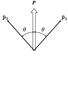
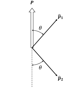
(a) (b)

Figure 1: Pictorial representation of the directions of muon polarization vector $\bm{P}$ and momentum of emitted electrons $\hat{p}_{i}$. (a) and (b) show the configurations where only $F_{S}$ and $F_{A}$ contribute, respectively. Here, three vectors, $\bm{P}$, $\hat{p}_{1}$, and $\hat{p}_{2}$, are in the same plane. $\theta$ is defined as an angle between $\bm{P}$ and $\hat{p}_{1}$. In (a), the vector $\hat{p}_{1}+\hat{p}_{2}$ is parallel to $\bm{P}$ so that the angle between $\hat{p}_{1}$ and $\hat{p}_{2}$ is $2\theta$. In (b), $\hat{p}_{1}+\hat{p}_{2}$ is perpendicular to $\bm{P}$ so that the angle between $\hat{p}_{1}$ and $\hat{p}_{2}$ is $\pi-2\theta$.

We consider the following cases in the single operator dominance hypothesis:

1. Contact interaction with scalar coupling, where the electrons are emitted with the same chirality:

   $$g_{1}=1,\hskip 2.84526ptA_{L/R}=0,\text{ and }g_{j\neq 1}=0.$$ (35)

2. Contact interaction with vector coupling, where the electrons are emitted with the same chirality:

   $$g_{3}=1,\hskip 2.84526ptA_{L/R}=0,\text{ and }g_{j\neq 1}=0.$$ (36)

3. Contact interaction, where the electrons are emitted with the opposite chirality:

   $$g_{5}=1,\hskip 2.84526ptA_{L/R}=0,\text{ and }g_{j\neq 5}=0.$$ (37)

4. Photonic interaction:

   $$A_{R}=1,\hskip 2.84526ptA_{L}=0,\text{ and }g_{j}=0.$$ (38)

In the following, we show results of asymmetry coefficients for a polarized muon in ²⁰⁸Pb. The muon and electron wave functions are obtained by solving a Dirac equation with a Coulomb potential of the uniform distribution of nuclear charge $\rho_{C}(r)$,

$$\rho_{C}(r)=\frac{3Ze}{4\pi R^{3}}\theta(R-r),$$ (39)

with $R=1.2A^{1/3}$fm, where $A$ is the mass number of the nucleus. The numerical results using a multipole expansion formula have been tested by comparing the results of a simple formula with the plane wave approximation.

The 2D plots of $F_{S}$ and $F_{A}$ for $g_{1}$, $g_{3}$, $g_{5}$, and $A_{R}$ as a function of electron energy $\epsilon_{1}$ and angle $c_{12}$ are shown in Fig. 2. It is sufficient to consider only the domain $0.5\leq\epsilon_{1}\leq 1$ for each function because, without loss of generality, the electron indices $i=1,2$ can be assigned so that $\epsilon_{1}\geq\epsilon_{2}$. The values of the asymmetry functions of $g_{2}$, $g_{4}$, $g_{6}$, and $A_{L}$ are just the opposite sign of those of $g_{1}$, $g_{3}$, $g_{5}$, and $A_{R}$ as discussed in the plane wave approximation. Figure 3 shows the $c_{12}$ dependence of $F_{S}$ for fixed $\epsilon_{1}$, and Fig. 4 shows the $\epsilon_{1}$-dependence of $F_{A}$ for fixed $c_{12}$. Depending on the CLFV interaction, the asymmetry functions can have a large value in a certain domain of $\epsilon_{1}$ and $c_{12}$. The asymmetry of photonic interaction $A_{R}$ is very different from those of contact interactions. Furthermore, the $g_{1}$ interaction can be distinguished from $g_{5}$ by using the $\epsilon_{1}$-$c_{12}$ dependence of $F_{S}$, while the asymmetry functions of $g_{1}$ are almost the same as those of $g_{3}$.

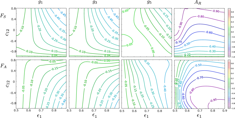
Figure 2: The asymmetry functions $F_{S}$(upper panel) and $F_{A}$(lower panel) for $g_{1}$, $g_{3}$, $g_{5}$, and $A_{R}$.

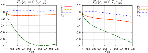
Figure 3: The asymmetry function $F_{S}$ for $g_{1}$, $g_{3}$, $g_{5}$, and $A_{R}$, where $\epsilon_{1}$ is fixed at $0.5$ (left panel) and $0.7$ (right panel).

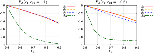
Figure 4: The asymmetry function $F_{A}$ for $g_{1}$, $g_{3}$, $g_{5}$, and $A_{R}$, where $c_{12}$ is fixed at $-1$ (left panel) and $-0.6$ (right panel).

The $F_{D}\bm{P}\cdot\left(\hat{p}_{1}\times\hat{p}_{2}\right)$ term is parity even but motion-reversal odd time_reversal . Nonzero $F_{D}$ could be used as a signal of the $CP$ violation of the CLFV interaction. However, it is known, for example in beta decay Ando2009 , that the final state interaction generates a motion-reversal-odd correlation. For the $\mu^{-}e^{-}\to e^{-}e^{-}$ process, the distortion effect of the emitted electrons by the nuclear potential also contributes to $F_{D}$. In order to quantitatively determine the $CP$ violating phases of CLFV interactions, it is necessary to evaluate the asymmetry stemming from effects other than the $CP$ violation and to correctly count them as background contributions.

Although coupling constants ($g_{j},A_{L/R}$) are taken to be real, the coefficient $F_{D}$ of the $\bm{P}\cdot\left(\hat{p}_{1}\times\hat{p}_{2}\right)$ term in Eq. (9) becomes nonzero due to the final state interaction. We concentrate on the final state interaction between each electron and nucleus, which has a much more significant effect than that between electrons because of the large nuclear charge. In the photonic interaction, an additional source of nonzero $F_{D}$ is the propagation of real and virtual photons in the intermediate state. Figure 5 shows the function $F_{D}$ as a function of $\epsilon_{1}$ and $c_{12}$. Since $\bm{P}\cdot\left(\hat{p}_{1}\times\hat{p}_{2}\right)$ is even under parity transformation, $F_{D}$ of $g_{1}$ is the same as that of $g_{2}$ in contrast to $F_{S}$ and $F_{A}$. $F_{D}$ is small for $g_{1}$ and $g_{3}$ and it has the largest value in photonic interactions. It is important to include the final state interaction properly in future searches for $CP$ violation of the CLFV interaction.

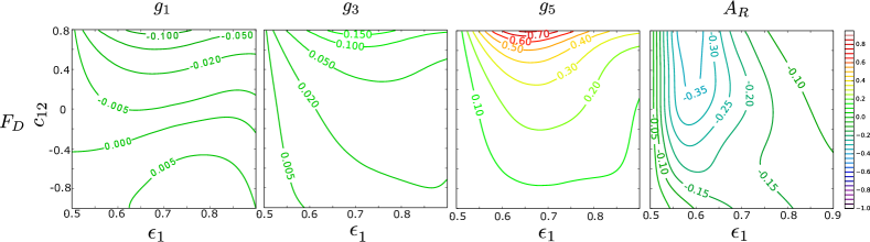
Figure 5: The asymmetry function $F_{D}$ for $g_{1}$, $g_{3}$, $g_{5}$, and $A_{R}$.

IV Conclusion

We have studied the energy-angular distributions of emitted electrons of $\mu^{-}e^{-}\to e^{-}e^{-}$ decay in a muonic atom with a polarized muon. The asymmetric distribution of electrons provides information about the CLFV interaction in addition to the atomic number dependence of the CLFV decay rate discussed in our previous works Uesaka2016 ; Uesaka2018 . Our findings are as follows: (i) The angular distribution of emitted electrons is a parity violating quantity. Therefore the asymmetry functions $F_{S}$ and $F_{A}$ probe the parity violation of CLFV interactions. (ii) The sign of the asymmetry directly reflects the chirality of the muon involved in the $\mu^{-}e^{-}\to e^{-}e^{-}$ process. (iii) Furthermore the $\epsilon_{1}$ and $c_{12}$ dependence of the asymmetry depends on the type of the CLFV operator in the effective Lagrangian, which would also be useful to distinguish models beyond the SM. In addition, it was found that the asymmetry could be large for the $\mu^{-}e^{-}\to e^{-}e^{-}$ process induced by the photonic dipole interaction.

We have also estimated the asymmetry coefficient of the motion-reversal-odd term assuming no $CP$ violating CLFV interactions. The asymmetry coefficient due to the final state interaction is not large, typically $O\left(10^{-2}\sim 10^{-1}\right)$.

In order to measure the asymmetry with enough precision we need a sufficient number of events. The $\mu^{-}e^{-}\to e^{-}e^{-}$ event rate is maximum at $\epsilon_{1}=0.5$ and $c_{12}=-1$ Uesaka2016 ; Uesaka2018 , where the asymmetry is zero. Therefore more careful study is needed to find an optimal kinematical condition to realize the idea and efforts are in progress.

Appendix A COMPLETE FORMULAS FOR DECAY RATE

In this appendix, we show the formulas for the differential decay rate where the initial muon is unpolarized, which have been already given in Refs. Uesaka2016 ; Uesaka2018 :

$$\frac{d^{2}\Gamma_{unpol.}}{d\epsilon_{1}dc_{12}}= \sum_{l\geq 0}c_{l}\left(\epsilon_{1}\right)P_{l}(c_{12}),$$ (40)

where $P_{l}(x)$ is the Legendre polynomial and the coefficient $c_{l}$ is

$$c_{l}\left(\epsilon_{1}\right)= \left(E_{tot}-2m_{e}\right)\frac{G_{F}^{2}}{2\pi^{3}}|\bm{p}_{1}||\bm{p}_{2}|\left(2j_{\kappa_{e}}+1\right)$$

$$\times\sum_{\kappa_{1},\kappa_{2}}\sum_{\kappa^{\prime}_{1},\kappa^{\prime}_{2}}\sum_{J}(-1)^{J-j_{\kappa_{2}}-j_{\kappa^{\prime}_{2}}}\frac{1+(-1)^{l_{\kappa_{1}}+l_{\kappa^{\prime}_{1}}+l}}{2}\frac{1+(-1)^{l_{\kappa_{2}}+l_{\kappa^{\prime}_{2}}+l}}{2}$$

$$\times i^{-l_{\kappa_{1}}-l_{\kappa_{2}}+l_{\kappa_{1}^{\prime}}+l_{\kappa_{2}^{\prime}}}e^{i\left(\delta_{\kappa_{1}}+\delta_{\kappa_{2}}-\delta_{\kappa_{1}^{\prime}}-\delta_{\kappa_{2}^{\prime}}\right)}N(J,\kappa_{1},\kappa_{2},E_{1},\alpha_{e})N^{*}(J,\kappa^{\prime}_{1},\kappa^{\prime}_{2},E_{1},\alpha_{e})$$

$$\times(2J+1)\left(2j_{\kappa_{1}}+1\right)\left(2j_{\kappa_{2}}+1\right)\left(2j_{\kappa_{1}^{\prime}}+1\right)\left(2j_{\kappa_{2}^{\prime}}+1\right)$$

$$\times\left(2l+1\right)\begin{pmatrix}j_{\kappa_{1}}&j_{\kappa^{\prime}_{1}}&l\\ 1/2&-1/2&0\end{pmatrix}\begin{pmatrix}j_{\kappa_{2}}&j_{\kappa^{\prime}_{2}}&l\\ 1/2&-1/2&0\end{pmatrix}\begin{Bmatrix}j_{\kappa_{1}}&j_{\kappa_{2}}&J\\ j_{\kappa^{\prime}_{2}}&j_{\kappa^{\prime}_{1}}&l\end{Bmatrix}.$$ (41)

The $N$ is represented by

$$N\left(J,\kappa_{1},\kappa_{2},E_{1},\alpha_{e}\right)=N_{\mathrm{photo}}+N_{\mathrm{contact}},$$ (42)

with

$$N_{\mathrm{photo}}= \sum_{j=L/R}A_{j}W_{j}(J,\kappa_{1},\kappa_{2},E_{1},\alpha_{e})$$ (43)

$$N_{\mathrm{contact}}= \sum_{j=1}^{6}g_{j}W_{j}(J,\kappa_{1},\kappa_{2},E_{1},\alpha_{e}).$$ (44)

Here the $W_{j}$’s ($j=1,2,\cdots,6$) for the contact interaction are given by

$$W_{1}(J)= \frac{1}{2}\left\{X^{-}_{\alpha}(J,0,J)-X^{+}_{\beta}(J,0,J)+i\left[Y^{+}_{\alpha}(J,0,J)+Y^{+}_{\beta}(J,0,J)\right]\right\},$$ (45)

$$W_{2}(J)= \frac{1}{2}\left\{X^{-}_{\alpha}(J,0,J)-X^{+}_{\beta}(J,0,J)-i\left[Y^{+}_{\alpha}(J,0,J)+Y^{+}_{\beta}(J,0,J)\right]\right\},$$ (46)

$$W_{3}(J)= 2\left\{X^{-}_{\alpha}(J,0,J)+X^{+}_{\beta}(J,0,J)-i\left[Y^{+}_{\alpha}(J,0,J)-Y^{+}_{\beta}(J,0,J)\right]\right\},$$ (47)

$$W_{4}(J)= 2\left\{X^{-}_{\alpha}(J,0,J)+X^{+}_{\beta}(J,0,J)+i\left[Y^{+}_{\alpha}(J,0,J)-Y^{+}_{\beta}(J,0,J)\right]\right\},$$ (48)

$$W_{5}(J)= 3\sum_{L=|J-1|}^{J+1}X^{-}_{\beta}(L,1,J)-X^{+}_{\alpha}(J,0,J)+i\left[3\sum_{L=|J-1|}^{J+1}Y^{-}_{\alpha}(L,1,J)+Y^{-}_{\beta}(J,0,J)\right],$$ (49)

$$W_{6}(J)= 3\sum_{L=|J-1|}^{J+1}X^{-}_{\beta}(L,1,J)-X^{+}_{\alpha}(J,0,J)-i\left[3\sum_{L=|J-1|}^{J+1}Y^{-}_{\alpha}(L,1,J)+Y^{-}_{\beta}(J,0,J)\right],$$ (50)

with

$$X^{\pm}_{\alpha}(L,S,J)= Z_{gggg}(L,S,J)+Z_{ffff}(L,S,J)\pm\left[Z_{gfgf}(L,S,J)+Z_{fgfg}(L,S,J)\right],$$ (51)

$$X^{\pm}_{\beta}(L,S,J)= Z_{ggff}(L,S,J)+Z_{ffgg}(L,S,J)\pm\left[Z_{gffg}(L,S,J)+Z_{fggf}(L,S,J)\right],$$ (52)

$$Y^{\pm}_{\alpha}(L,S,J)= Z_{ggfg}(L,S,J)-Z_{ffgf}(L,S,J)\pm\left[Z_{fggg}(L,S,J)-Z_{gfff}(L,S,J)\right],$$ (53)

$$Y^{\pm}_{\beta}(L,S,J)= Z_{gggf}(L,S,J)-Z_{fffg}(L,S,J)\pm\left[Z_{gfgg}(L,S,J)-Z_{fgff}(L,S,J)\right],$$ (54)

and

$$Z_{ABCD}(L,S,J)= \int_{0}^{\infty}drr^{2}A_{p_{1}}^{\kappa_{1}}(r)B_{1,\mu}^{\kappa_{\mu}}(r)C_{p_{2}}^{\kappa_{2}}(r)D_{n,e}^{\kappa_{e}}(r)$$

$$\times\sqrt{\left(2l^{A}_{\kappa_{1}}+1\right)\left(2l^{B}_{\kappa_{\mu}}+1\right)\left(2l^{C}_{\kappa_{2}}+1\right)\left(2l^{D}_{\kappa_{e}}+1\right)}$$

$$\times\left(l^{A}_{\kappa_{1}},0,l^{C}_{\kappa_{2}},0|L,0\right)\left(l^{B}_{\kappa_{\mu}},0,l^{D}_{\kappa_{e}},0|L,0\right)$$

$$\times\begin{Bmatrix}l^{A}_{\kappa_{1}}&1/2&j_{\kappa_{1}}\\ l^{C}_{\kappa_{2}}&1/2&j_{\kappa_{2}}\\ L&S&J\end{Bmatrix}\begin{Bmatrix}l^{B}_{\kappa_{\mu}}&1/2&j_{\kappa_{\mu}}\\ l^{D}_{\kappa_{e}}&1/2&j_{\kappa_{e}}\\ L&S&J\end{Bmatrix},$$ (55)

where $\kappa_{\mu}=-1$. Here $A$ and $C$ represent the electron scattering states with momenta $p_{1}$ and $p_{2}$, and $B$ and $D$ represent the bound states of the muon and electron. The radial wave functions $A(r)$, $B(r)$, $C(r)$, and $D(r)$ are either $g(r)$ or $f(r)$. The angular momentum $l^{h}_{\kappa}$ is defined as

$$l^{h}_{\kappa}=\begin{cases}l_{+\kappa}&\ \mbox{for}\ \ h=g,\\ l_{-\kappa}&\ \mbox{for}\ \ h=f.\end{cases}$$ (56)

The amplitudes of the photonic interaction $W_{L/R}$ are given as

$$W_{L/R}= \frac{2m_{\mu}}{i}\sqrt{\pi\alpha}\sum_{l=0}^{\infty}\sum_{j=|l-1|}^{l+1}\sum_{\lambda=1}^{3}\left[X_{\lambda}\left(l,j,\kappa_{1},\kappa_{2},J\right)\pm iY_{\lambda}\left(l,j,\kappa_{1},\kappa_{2},J\right)\right],$$ (57)

where $\pm$ corresponds to $L$ and $R$, respectively. $X_{\lambda}$ and $Y_{\lambda}$ are expressed in terms of $Z$ as

$$X_{1}\left(l,j,\kappa_{1},\kappa_{2},J\right)= (-1)^{l+j}\left\{Z_{gfgf}^{l,l,1,j}(J)+Z_{fggf}^{l,l,1,j}(J)-Z_{gffg}^{l,l,1,j}(J)-Z_{fgfg}^{l,l,1,j}(J)\right\},$$ (58)

$$X_{2}\left(l,j,\kappa_{1},\kappa_{2},J\right)= f_{l-j}^{(2)}(j)\left\{Z_{gfgg}^{l,j,0,j}(J)+Z_{fggg}^{l,j,0,j}(J)+Z_{gfff}^{l,j,0,j}(J)+Z_{fgff}^{l,j,0,j}(J)\right\},$$ (59)

$$X_{3}\left(l,j,\kappa_{1},\kappa_{2},J\right)= f_{l-j}^{(3)}(j)\sum_{\{l_{a},l_{b}\}=\{l,j\},\{j,l\}}\left\{Z_{gggf}^{l_{a},l_{b},1,j}(J)-Z_{ffgf}^{l_{a},l_{b},1,j}(J)-Z_{ggfg}^{l_{a},l_{b},1,j}(J)+Z_{fffg}^{l_{a},l_{b},1,j}(J)\right\},$$ (60)

$$Y_{1}\left(l,j,\kappa_{1},\kappa_{2},J\right)= (-1)^{l+j}\left\{Z_{gggf}^{l,l,1,j}(J)-Z_{ffgf}^{l,l,1,j}(J)-Z_{ggfg}^{l,l,1,j}(J)+Z_{fffg}^{l,l,1,j}(J)\right\},$$ (61)

$$Y_{2}\left(l,j,\kappa_{1},\kappa_{2},J\right)= f_{l-j}^{(2)}(j)\left\{Z_{gggg}^{l,j,0,j}(J)-Z_{ffgg}^{l,j,0,j}(J)+Z_{ggff}^{l,j,0,j}(J)-Z_{ffff}^{l,j,0,j}(J)\right\},$$ (62)

$$Y_{3}\left(l,j,\kappa_{1},\kappa_{2},J\right)= f_{l-j}^{(3)}(j)\sum_{\{l_{a},l_{b}\}=\{l,j\},\{j,l\}}\left\{Z_{gffg}^{l_{a},l_{b},1,j}(J)+Z_{fgfg}^{l_{a},l_{b},1,j}(J)-Z_{gfgf}^{l_{a},l_{b},1,j}(J)-Z_{fggf}^{l_{a},l_{b},1,j}(J)\right\},$$ (63)

where

$$f_{h}^{(2)}(j)=\begin{cases}\sqrt{\dfrac{j+1}{2j+1}}&(h=+1)\\ 0&(h=0)\\ \sqrt{\dfrac{j}{2j+1}}&(h=-1)\end{cases},\hskip 28.45274ptf_{h}^{(3)}(j)=\begin{cases}\sqrt{\dfrac{j}{2j+1}}&(h=+1)\\ 0&(h=0)\\ -\sqrt{\dfrac{j+1}{2j+1}}&(h=-1)\end{cases}.$$ (64)

The matrix element $Z$, which consists of the CLFV and the electromagnetic vertex and the photon propagator, is given by

$$Z_{ABCD}^{l_{a},l_{b},s,j}(J)= \left[q_{0}^{2}\int_{0}^{\infty}dr_{1}r_{1}^{2}A_{p_{1}}^{\kappa_{1}}(r_{1})B_{1,\mu}^{\kappa_{\mu}}(r_{1})\int_{0}^{\infty}dr_{2}r_{2}^{2}F_{l_{a},l_{b}}^{q_{0}}(r_{1},r_{2})C_{p_{2}}^{\kappa_{2}}(r_{2})D_{n,e}^{\kappa_{e}}(r_{2})\right.$$

$$\left.\times(-1)^{J+\kappa_{1}+\kappa_{\mu}}V_{l_{a},1,j}^{s_{A}\kappa_{1},s_{B}\kappa_{\mu}}V_{l_{b},s,j}^{s_{C}\kappa_{2},s_{D}\kappa_{e}}\begin{Bmatrix}j_{\kappa_{1}}&j_{\kappa_{2}}&J\\ j_{\kappa_{e}}&j_{\kappa_{\mu}}&j\end{Bmatrix}\right]$$

$$-(-1)^{j_{\kappa_{1}}+j_{\kappa_{2}}-J}\left[\left\{p_{1},\kappa_{1}\right\}\leftrightarrow\left\{p_{2},\kappa_{2}\right\}\right],$$ (65)

where $\kappa_{\mu}=-1$ again. $q_{0}$ is $q_{0}=m_{\mu}-B_{\mu}^{1s}-E_{1}$ for the direct term, and $q_{0}=m_{\mu}-B_{\mu}^{1s}-E_{2}$ for the exchange term. The coefficients $V$ are given by

$$V_{l,s,j}^{\kappa_{b},\kappa_{a}}= (-1)^{l}\frac{1+(-1)^{l_{\kappa_{b}}+l_{\kappa_{a}}+l}}{2}\left(j_{\kappa_{b}},1/2,j_{\kappa_{a}},-1/2|j,0\right)$$

$$\times\begin{cases}\delta_{l,j}&(s=0,j=l)\\ (j-\kappa_{a}-\kappa_{b})/\sqrt{j(2j+1)}&(s=1,j=l+1)\\ (\kappa_{a}-\kappa_{b})/\sqrt{j(j+1)}&(s=1,j=l)\\ -(j+1+\kappa_{a}+\kappa_{b})/\sqrt{(j+1)(2j+1)}&(s=1,j=l-1)\end{cases}.$$ (66)

We use $s_{A}=\pm 1$ for $A=g$ and $A=f$, respectively. $F_{l_{a},l_{b}}^{q_{0}}(r_{1},r_{2})$ is the coefficient in the partial wave expansion of the photon propagator, which is given as

$$\int\frac{d^{3}q}{(2\pi)^{3}}\frac{q_{\nu}e^{-i\bm{q}\cdot\left(\bm{r}_{1}-\bm{r}_{2}\right)}}{|\bm{q}|^{2}-q_{0}^{2}-i\epsilon}=q_{0}\partial_{\nu}\sum_{l,m}Y_{l}^{m*}\left(\hat{r}_{1}\right)Y_{l}^{m}\left(\hat{r}_{2}\right)F_{l,l}^{q_{0}}\left(r_{1},r_{2}\right),$$ (67)

where we have defined $\partial_{\nu}=(iq_{0},\bm{\nabla}_{1})$ and

$$F_{l_{1},l_{2}}^{q_{0}}\left(r_{1},r_{2}\right)=h_{l_{1}}^{(1)}\left(q_{0}r_{1}\right)j_{l_{2}}\left(q_{0}r_{2}\right)\theta(r_{1}-r_{2})+h_{l_{2}}^{(1)}\left(q_{0}r_{2}\right)j_{l_{1}}\left(q_{0}r_{1}\right)\theta(r_{2}-r_{1}).$$ (68)

Here $j_{l}$ and $h_{l}^{(1)}$ are the spherical Bessel function and the first kind spherical Hankel function, respectively.