Sampling first-passage times of fractional Brownian Motion using adaptive bisections

Abstract

We present an algorithm to efficiently sample first-passage times for fractional Brownian motion. To increase the resolution, an initial coarse lattice is successively refined close to the target, by adding exactly sampled midpoints, where the probability that they reach the target is non-negligible. Compared to a path of $N$ equally spaced points, the algorithm achieves the same numerical accuracy $N_{\rm eff}$, while sampling only a small fraction of all points. Though this induces a statistical error, the latter is bounded for each bridge, allowing us to bound the total error rate by a number of our choice, say $P_{\rm error}^{\rm tot}=10^{-6}$. This leads to significant improvements in both memory and speed. For $H=0.33$ and $N_{\rm eff}=2^{32}$, we need $5\,000$ times less CPU time and $10\,000$ times less memory than the classical Davies Harte algorithm. The gain grows for $H=0.25$ and $N_{\rm eff}=2^{42}$ to $3\cdot 10^{5}$ for CPU and $10^{6}$ for memory. We estimate our algorithmic complexity as ${\cal C}^{\rm ABSec}(N_{\rm eff})={\cal O}\left(\left(\ln N_{\rm eff}\right)^{3}\right)$, to be compared to Davies Harte which has complexity ${\cal C}^{\rm DH}(N)={\cal O}\left(N\ln N\right)$. Decreasing $P_{\rm error}^{\rm tot}$ results in a small increase in complexity, proportional to $\ln(1/P_{\rm error}^{\rm tot})$. Our current implementation is limited to the values of $N_{\rm eff}$ given above, due to a loss of floating-point precision. Our algorithm can be adapted to other extreme events and arbitrary Gaussian processes. It enables one to numerically validate theoretical predictions that were hitherto inaccessible.

I Introduction

Estimating the distribution of first-passage times is a key problem in understanding systems as different as financial markets or biological systems Redner2001 ; Metzler2014 , and the dynamics of local reactions Haenggi1990 ; GodecMetzler2016 . Typically, research focuses on non-Markovian processes and bounded geometries, where first-passage time distributions are difficult to obtain analytically Sanders2012 ; Guerin2016 ; Levernier2018 ; Wiese2018 ; ArutkinWalterWiese2019 . Within the class of non-Markovian processes, fractional Brownian Motion (fBm) is of particular interest as it naturally extends standard diffusion to sub- and super-diffusive self-similar processes MandelbrotVanNess1968 . Fractional Brownian Motion is a one-parameter family of Gaussian processes, indexed by the Hurst parameter $H\in(0,1]$. The latter parametrizes the mean-square displacement via

$$\left\langle X_{t}^{2}\right\rangle=2t^{2H}\ ,$$ (1)

recovering standard Brownian Motion at $H=\frac{1}{2}$. It retains from Brownian motion scale and translational invariance, both in space and time.

In order to render the extreme events of this process accessible to an analytical treatment, an $\varepsilon$-expansion around Brownian motion in $\varepsilon=H-\frac{1}{2}$ has been proposed WieseMajumdarRosso2010 . This field theoretic approach has been applied to a variety of extreme events, yielding the first-order corrections of several probability distributions WieseMajumdarRosso2010 ; DelormeWiese2015 ; SadhuDelormeWiese2017 ; Wiese2018 . The scaling functions predicted by this perturbative field theory are computationally expensive to verify, since they require a high numerical resolution of the path. Typically this is done by simulating a discretized version of the path over a grid of $N$ equidistant points. Measuring a first-passage time then amounts to finding the first passage of a linear interpolation of these grid points. This approximation, however, can lead to a systematic over-estimation of the first-passage time. As can be seen on Fig. 1, a high resolution of the path is necessary in order to find the first-passage event at $t=0.36$ instead of the one at $t=0.45$ or even $t=0.47$ for the coarser grids. To account for this, usually the number of grid points is increased. As the size of fluctuations between gridpoints diminishes as

$$\delta X=N^{-H}\ ,$$ (2)

the sub-diffusive regime ($H<\frac{1}{2}$) necessitates an enormous computational effort.

Figure 1: The continuous stochastic path (grey) crosses the barrier (blue) for the first time at $\tau^{\infty}$ (black square mark). The discretization with $N$ points (red) over-estimates this time as $\tau^{N}$ (red square). The numerical estimate is improved to $\tau^{4N}$ (green square) when refining the discretization (green). This systematic error worsens for diminishing values of Hurst parameter $H$.

As can be seen in Ref. Wiese2018 , this poses challenges to the numerical validation of high-precision analytical predictions. As an example, for $H=0.33$, one needs system sizes of at least $N=2^{24}$, necessitating a CPU time of 6 seconds per sample. If theories of such high precision are to be tested against simulations, new numerical techniques need to be developed. The present work addresses this problem by designing, implementing, and benchmarking a new algorithm sampling first-passage times of fractional Brownian Motion using several orders of magnitude less CPU time and memory than traditional methods. The general idea is to start from a rather coarse grid (as the red one on Fig. 1), and to refine the grid where necessary. As a testing ground, we simulate and compare to theory the first-passage time of an fBm with drift ArutkinWalterWiese2019 .

The algorithm proposed here is an adaptive bisection routine that draws on several numerical methods already established in this field, notably the Davies-Harte algorithm DaviesHarte1987 , bisection methods Ceperley1995 ; Sprik1985 , and the Random Midpoint Displacement method Fournier1982 ; Norros2004 . The central, and quite simple, observation is that in order to resolve a first-passage event it is necessary to have a high grid resolution only near the target. This translates into an algorithm that generates a successively refined grid, where refinement takes place only at points close to the target, with the criterion of closeness scaling down by $2^{{-H}}$ for each bisection. This refinement is stopped after the desired resolution is reached. The sampling method is exact, i.e. the collection of points is drawn from the ensemble of fBm, a continuous process, with no bias. The only error one can make is that one misses an intermediate point. We have been able to control this error with a failure rate smaller than $10^{-6}$ per realisation.

While there is a relatively large overhead for the non-homogenous refinement, this is compensated by the use of far less points, leading to a significant increase both in speed and memory efficiency over sampling methods that produce points for the full grid. For $H=0.33$ and system size $N=2^{32}$, our algorithm is 5000 times faster than the Davies Harte Algorithm (DH), the fastest exact sampler (cf. DiekerPhD ; Craigmile2003 ) if all points are needed. It has computational complexity $\mathcal{O}(N\log(N))$, which makes it the standard algorithm in most current works, see e.g. Guerin2016 ; Levernier2018 ; Krapf2019 , with system size $N$ ranging from $2^{21}$ to $2^{24}$. Our maximal grid size is limited by the precision of the floating point unit to $N_{\rm max}\approx 2^{11/H}$.

This paper is organised as follows. In Sec. II, we introduce our adaptive bisection algorithm. First, its higher-level structure is outlined and then each subroutine is detailed. Possible generalisations to other extreme events or other Gaussian processes are discussed at the end of this section. In Sec. III, we present our implementation of the adaptive bisection in C, which is freely available WalterWiese2019a . We benchmark it against an implementation of the Davies Harte algorithm. We compare error rates, average number of bisections, CPU time and memory. Sec. IV contains a summary of our findings.

II Algorithm

In this section, we introduce the adaptive bisection routine (ABSec). The central aim is to translate the idea of refining the grid “where it matters” into a rigorous routine.

II.1 Fractional Brownian Motion and first-passage times

Gaussian processes $X_{t}$ are stochastic processes for which $X_{t}$ evaluated at a finite number of points ${\cal T}$ in time, has a multivariate Gaussian distribution Piterbarg2015 . They are simple to handle, since their path probability measure can be obtained from their correlation function. The best known Gaussian Process is Brownian Motion which is the only translational invariant Gaussian process with stationary and independent increments.

Fractional Brownian Motion (fBm) generalises Brownian Motion by relaxing the requirement of independent increments, while keeping self-similarity. The latter property means that its path probability measure is invariant under a space-time transformation $t\to ct,\ x\to c^{-H}x$ for $c>0$. The parameter $H$ is referred to as Hurst exponent. As a Gaussian process, fBm is entirely characterized by its mean $X_{0}=\left\langle X_{t}\right\rangle=0$, and correlation function

$$C(s,t)=\left\langle X_{s}X_{t}\right\rangle=|s|^{2H}+|t|^{2H}-|t-s|^{2H}\ ,$$ (3)

where $H\in(0,1]$. As a consequence, $\left\langle(X_{t}-X_{s})^{2}\right\rangle=2|t-s|^{{2H}}$, and in particular $\left\langle X_{t}^{2}\right\rangle=2|t|^{{2H}}$. From the correlation function it follows that on all time scales non-overlapping increments are positively correlated for $H>\frac{1}{2}$ and negatively correlated for $H<\frac{1}{2}$. For $H=\frac{1}{2}$ one recovers Brownian Motion with uncorrelated increments.

The first-passage time (FPT) of a stochastic process is the fist time the process crosses a threshold $m$. Since we use $X_{0}=0$, it is defined for $m>0$ as

$$\tau_{m}=\inf_{t>0}\left\{t|X_{t}\geq m\right\}.$$ (4)

II.2 Notation

In simulating a fBm on a computer, one is forced to represent the continuous path by a discretized path that takes values on a finite set of points in time, the grid. We denote the grid by ordered times $\mathcal{T}=\left\{t_{1},t_{2},\cdots,t_{N}\right\}$, and the corresponding values of the process by $\mathcal{X}=\left\{X_{t_{1}},X_{t_{2}},\cdots,X_{t_{N}}\right\}$. Together, $(\mathcal{X},\mathcal{T})$ form the discretized path. Due to self-similarity of the process, we can restrict ourselves to $\mathcal{T}\subset[0,1]$ with no loss of generality. The intervals between any two successive times $t_{i},t_{i+1}\in\mathcal{T}$ are referred to as bridges $(t_{i},t_{i+1})$. Each connected component of $[0,1]\backslash\mathcal{T}$ is a bridge.

We denote the dyadic lattice on the unit interval by $\Lambda^{k}=\left\{i\cdot 2^{-k};0\leq i\leq 2^{k}\right\}$. Our adaptive bisection algorithm sets out from a dyadic lattice $\mathcal{T}^{(0)}=\Lambda^{g}$ of relatively low resolution (typically $g\lesssim 8$ or 10) and performs several bisections of that grid in successive iterations $\mathcal{T}^{(0)},\mathcal{T}^{(1)},\cdots,\mathcal{T}^{(M)}$, where $M$ is the number of bisections generated before the routine terminates. To each bridge $(t_{\rm l},t_{\rm r})$ spanned in between left and right endpoints $t_{\rm l}$ and $t_{\rm r}$ and contained in a grid $\mathcal{T}^{(m)}$, one can associate a level $\ell$ defined by $\ell=-\log_{2}\left(t_{\rm r}-t_{\rm l}\right)$. A bridge is bisected by introducing its midpoint, $t_{\rm m}=\frac{1}{2}\left(t_{\rm l}+t_{\rm r}\right)=t_{\rm l}+2^{-\ell-1}$ and inserting it into the grid $\mathcal{T}^{(m+1)}=\left\{t_{1},...,t_{\rm l},t_{\rm m},t_{\rm r},...,t_{N}\right\}$. A bridge is allowed to be bisected until the level of a bridge reaches a maximum bisection level $L$ (typically $L\lesssim 30$ for $H=0.33$). Since each iteration only halves an existing interval, all grids are sandwiched between two dyadic lattices

$$\Lambda^{g}=\mathcal{T}^{(0)}\subset\mathcal{T}^{(1)}\subset\cdots\subset\mathcal{T}^{(M)}\subseteq\Lambda^{L},$$ (5)

representing the lowest and highest possible resolution. We define the truncation of the grid $\mathcal{T}$ to a certain time $\tau\in[0,1]$ as

$${\cal T}|_{\tau}:=\left\{t_{i}\in\mathcal{T}|t_{i-1}<\tau\right\}$$ (6)

i.e. the truncation contains all points in time up to time $\tau$ and to the next highest gridpoint contained in the initial grid $\Lambda^{g}$ (cf. section II.3.3). Note that for each bridge $(t_{\rm l},t_{\rm r})$, there is always one dyadic lattice $\Lambda^{n}$, s.t. $t_{i}$ and $t_{i+1}$ are neighbouring points in $\Lambda^{n}$; they are members, but not neighbours in $\Lambda^{n^{\prime}}$ for $n^{\prime}>n$, and at least one of them does not exist in $\Lambda^{n^{\prime}}$ for $n^{\prime}<n$.

II.3 Definition of the algorithm

The algorithm consists of two phases. In the first phase, the initialisation, a coarse grid is generated. In the second phase, the adaptive bisection, this grid is successively bisected where necessary. Once the second phase terminates, the first-passage time is calculated using the final grid.

The first phase starts by sampling an initial discretized path $\mathcal{X}^{(0)}$ over a dyadic lattice $\mathcal{T}^{(0)}=\Lambda^{g}$ with $N=2^{g}$ equidistant points, using the Davies-Harte salgorithm. The latter is the fastest known algorithm to sample an exact fBm path on an equidistant grid in time DiekerPhD : its execution time scales as $N\ln(N)$, thus only slightly slower than what is needed to generate an uncorrelated sample of the same length $N$. From this relatively coarse grid, $(\mathcal{X}^{(0)},\mathcal{T}^{(0)})$, the first-passage time is estimated via linear interpolation as $\tau^{(0)}$.

Subsequently, the grid is truncated by discarding all points behind the first point surpassing $m$ (cf. Eq. (6)). That this does not change the measure is explained in section II.3.3. If no such point exists, the full grid is kept. The correlations between the different points $X_{t}$ at times $t$ stored in the grid are given by the correlation matrix

$$C_{ij}(\mathcal{T})=C(t_{i},t_{j})\ ,\qquad t_{i},t_{j}\in\mathcal{T},1\leq i,j\leq|\mathcal{T}|\ .$$ (7)

It is a symmetric matrix computed from the correlation function (3). It is then inverted to obtain the inverse correlation matrix $C^{-1}_{ij}(\mathcal{T})$. The inversion is optimised by using pre-calculated tabularized matrices. This concludes the first phase.

In the second phase, bridges are checked successively until the maximum level is reached. The order in which the bridges of the growing grid are checked is determined by a subroutine whose aim is to find the first-passage event with the least amount of bisections. The check consists in testing whether the midpoint $X_{t_{\rm m}}$ of the bridge $(t_{\rm l},t_{\rm r})$ could surpass the threshold $m$ with a probability larger than $\varepsilon$, taken small. If this is the case the bridge is deemed critical and bisected. The bisection consists in generating a midpoint $X_{t_{\rm m}}$ at time $t_{\rm m}$ conditional to the pre-existing grid. This computation requires the inverse correlation matrix and is detailed in Sec. II.3.6. Once the midpoint is generated, it is added to the path $(\mathcal{X},\mathcal{T})$. In a last step the inverse correlation matrix of the new grid, $C^{-1}(\mathcal{T}\cup t_{\rm m})$ is stored. Further below, the algorithm is given in pseudocode.

 

ALGORITHM 1: Adaptive bisection

 

procedure ABSec($g,L,m,\varepsilon$)

     $\mathcal{T}\leftarrow\Lambda^{g}$

     $\mathcal{X}\leftarrow$davies_harte($\Lambda^{g}$) $\triangleright$ II.3.1

     $\tau\leftarrow$ fpt_from_grid($\mathcal{X},\mathcal{T}$) $\triangleright$ II.3.2

     $(\mathcal{X},\mathcal{T})\leftarrow\left.(\mathcal{X},\mathcal{T})\right|_{\tau^{(0)}}$ $\triangleright$ II.3.3

     $C^{-1}\leftarrow$ CMatrixTable[$\tau^{(0)}$] $\triangleright$ II.3.4

     $(t_{\rm l},t_{\rm r})\leftarrow$Next bridge($\mathcal{T}$, 0, $\tau^{(0)}$)

     while $(t_{\rm l},t_{\rm r})$ defined do

         if Bridge $(t_{\rm l},t_{\rm r})$ critical and not yet bisected then $\triangleright$ II.3.5

              $C^{-1}\leftarrow\textsc{Augment ${C^{-1}}$-Matrix}(C^{-1},t_{\rm m})$

              $X^{*}\leftarrow\textsc{Generate midpoint}(C^{-1},t_{\rm m})$ $\triangleright$ II.3.6

              $\mathcal{X}\leftarrow\mathcal{X}\cup X^{*}$

              $\mathcal{T}\leftarrow\mathcal{T}\cup t_{\rm m}$

              if $X^{*}>m$ then

                  $\tau\leftarrow\textsc{fpt\_from\_grid}(\mathcal{X},\mathcal{T})$                        

         $(t_{i},t_{i+1})\leftarrow$Next bridge($\mathcal{T}$, $(t_{i},t_{i+1})$, $\tau$) $\triangleright$ II.3.7      

     output($\tau$)

 

The routines in the pseudocode are described in sections II.3.1–II.3.7.

II.3.1 Davies-Harte Algorithm

The Davies-Harte algorithm (DH) is a widely used method to generate fBm samples. It was introduced in DaviesHarte1987 , is pedagogically described in DiekerPhD , and has been extended to other Gaussian processes in Craigmile2003 , allowing us to omit an introduction. It generates a sample of fractional Gaussian noise (fGn) $\xi_{1},\xi_{2},\cdots,\xi_{N}$, the incremental process of fBm $\xi_{j}=X_{j+1}-X_{j},j\in\mathbb{N}$, and then sums the increments to a fBm sample with values $X_{i\cdot\delta t}=(\delta t)^{H}\sum_{j=1}^{i}\xi_{j}$. Simulating the increments is more efficient since fGn is a stationary Gaussian process which, for equally sized increments, has a circulant correlation matrix, which can be diagonalised using a fast Fourier transform (FFT). Therefore a fGn sample of $N$ increments can be simulated with computational complexity $\mathcal{O}(N\log(N))$. The FFT algorithm works optimally when the number of points is a natural power of $2$, i.e. if the grid is a dyadic lattice.

II.3.2 Estimating the first-passage time

Given a discretized path $(\mathcal{X},\mathcal{T})$, we use its linear interpolation to give the first-passage time as its first intersection with the threshold (cf. Fig.1).

II.3.3 Truncating the grid

A further optimisation is to discard grid points beyond the first point crossing the threshold (cf. Eq. (6)). It is necessary to show that the density of first-passage times conditioned on the full grid equals the distribution conditioned on the truncated grid, i.e. that truncating does not change the measure.

The first-passage time distribution (FPTD) $P(\tau)$ can be decomposed into a sum of conditional probabilities for disjoint events: Each term of the sum is the probability that the $i$th point of a grid surpasses $m$, the threshold, for the first time (“$P^{\rm grid}(X_{t_{i}}>m\text{ first})$”), times the FPTD of a fBm conditioned on the event that its discretization on grid $\mathcal{T}$ surpasses $m$ at $t_{i}$ for the first time, i.e.

$$P_{\mathcal{T}}(\tau|X_{t_{i}}>m\text{ first})\\ =P(\tau|X_{t}:X_{t_{i}}>m\text{ and }X_{t_{j}}<m\,\forall t_{j}<t_{i})$$ (8)

for $t_{j},t_{i}\in\mathcal{T}$. The decomposition thus reads

$$P(\tau)=\sum_{t_{i}\in\mathcal{T}}P_{\mathcal{T}}(\tau|X_{t_{i}}>m\text{ first})P^{\rm grid}(X_{t_{i}}>m\text{ first}).$$ (9)

By continuity of the process,

$$P_{\mathcal{T}}(\tau>t_{i}|X_{t_{i}}>m\text{ first})=0,$$ (10)

such that the sum in Eq. (9) can be truncated to

$$P(\tau)=\sum_{t_{i-1}<\tau}P_{\mathcal{T}}(\tau|X_{t_{i}}>m\text{ first})P^{\rm grid}(X_{t_{i}}>m\text{ first}).$$ (11)

In order to sample $P_{\mathcal{T}}(\tau|X_{t_{i}}>m\text{ first})$, one would naively sample the entire grid $\mathcal{X}$ over all of $\mathcal{T}$, but since

$$P_{\mathcal{T}}(\tau|X_{t_{i}}>m\text{ first})=P_{\mathcal{T}|_{\tau}}(\tau|X_{t_{i}}>m\text{ first}),$$ (12)

where the restriction is defined in Eq. (6), it is sufficient to only regard the smaller grid $\mathcal{T}|_{\tau}$, i.e.

$$P(\tau)=\sum_{t_{i-1}<\tau}P_{\mathcal{T}|_{\tau}}(\tau|X_{t_{i}}>m\text{ first})P^{\rm grid}(X_{t_{i}}>m\text{ first}).$$ (13)

Discarding points in the initial stage leads to a smaller correlation matrix to be inverted, which increases performance, and decreases memory.

II.3.4 Tabulating inverse correlation matrices

The inverse of the correlation matrix (7) is necessary to compute the conditional probability of any further midpoint (cf. App. B). Its computation is costly and typically scales with $\mathcal{O}(N^{3})$ where $N=2^{g}$ is the number of points in $\mathcal{T}^{(0)}$. If the algorithm is run multiple times, this computation slows it down. The initial grid however, is always a dyadic lattice truncated at some point, i.e. $\mathcal{T}^{(0)}=\left\{k2^{-g};0\leq k\leq K\right\}$, where $X_{K2^{-g}}$ is the first point to surpass $m$. Therefore, the initial inverse correlation matrix $C^{-1}\left(\mathcal{T}^{(0)}\right)$ can take $2^{g}-1$ possible values, one for each possible value of $K$. It is more efficient to pre-calculate all possible inverse correlation matrices in the beginning, and store them in a vector ‘CMatrixTable’,

$$\mathtt{CMatrixTable}[K]=\left(\left[C(i\cdot 2^{-g},j\cdot 2^{-g})\right]_{i,j=1}^{K}\right)^{-1}\ .$$ (14)

After generating the initial grid and measuring $\tau^{(0)}$, one reads out the appropriate entry of the table at $K=\min\left\{n\in\mathbb{Z};n2^{-g}\geq\tau^{(0)}\right\}$.

II.3.5 Deciding whether a bridge is critical

Once entering the bisection phase, the algorithm needs to decide whether a particular bridge is critical, i.e. whether it is suspicious of hiding a “dangereous” excursion crossing the threshold at $m$ (cf. Fig. 1). Rather than determining whether any point in $(t_{\rm l},t_{\rm r})$ surpasses the threshold, we focus on the midpoint $t_{\rm m}$ conditioned on all other points $\mathcal{X}$, and ask how likely $X_{t_{\rm m}}>m$. Such an event needs to be avoided with a very low probability $\varepsilon$, the error tolerance. The relevant probability,

$$P\left(X_{t_{\rm m}}>m|\mathcal{X}\right)<\epsilon,$$ (15)

is too costly to be computed for every bridge in every step of the iteration, as the midpoint is a Gaussian random variable, with its mean and variance determined by every other point in the grid. If we ignore all points of the path apart from $(t_{i},X_{t_{i}})$ and $(t_{i+1},X_{t_{i+1}})$, a calculation given in App. A shows that mean and variance would be given by

$$\mu=\frac{1}{2}\left(X_{t_{i}}+X_{t_{i+1}}\right)$$ (16)

and

$$\sigma^{2}=\left(2^{1-2H}-\frac{1}{2}\right)\times 2^{-2\ell H}\ .$$ (17)

Here $\ell$ is the level of the bridge of width $\delta t=2^{-\ell}$. Interestingly, adding to the bridge’s endpoints further points lowers the variance (cf. Eq. (30)) which means that neglecting all but nearest neighbours gives an upper bound on the variance of the midpoint. Further, we conservatively bound the mean by the maximum of both endpoints, $\mu\lesssim\max\left(X_{t_{i}},X_{t_{i+1}}\right)$. This is a priori not a precise approximation, since far-away grid points are able to “push” the expected midpoint above the bridges’ endpoints for values of $H\neq\frac{1}{2}$. As is shown in Sec. III.3, this systematic error can be absorbed by introducing an even smaller error tolerance $\varepsilon^{\prime}$. Furthermore, it is less relevant in the sub-diffusive regime, where the process is negatively correlated. By giving conservative bounds on mean and variance with quantities that are local (i.e. do not depend on the remaining grid), we can replace the original criterion (15) by a computationally cheaper alternative, namely the local condition

$$P\left(X_{t_{\rm m}}>m|(X_{t_{\rm l}},X_{t_{\rm r}})\right)<\epsilon^{\prime}.$$ (18)

This implies that Eq. (15) holds for an appropriate choice of $\varepsilon^{\prime}$, on average. This is to be understood as follows: In a simulation, there are $n$ decisions of type (15) to be taken. The total error is approximately $P_{\rm error}^{\rm tot}\approx n\epsilon$. The parameter $\epsilon^{\prime}$ is chosen such that the total error rate remains smaller than $10^{-6}$, and thus negligible as compared to MC fluctuations. The dependence between $\epsilon^{\prime}$ and $P_{\rm error}^{\rm tot}$ is investigated in Sec. III.3 (cf. Fig. 3).

Criterion (18) is rephrased, using again $\ell$ as the level of the bridge, to

$$\Phi\left(\frac{m-\max\left(X_{t_{i}},X_{t_{i+1}}\right)}{\left(\sqrt{2^{1-2H}-\frac{1}{2}}\right)2^{-\ell H}}\right)>1-\varepsilon^{\prime}$$ (19)

which implies

$$\max\left(X_{t_{i}},X_{t_{i+1}}\right)<m-\left(\sqrt{2^{1-2H}{-}\frac{1}{2}}\right)2^{-\ell H}\Phi^{-1}(1{-}\varepsilon^{\prime}),$$ (20)

where we introduced $\Phi$, the cumulative distribution function of the standard normal distribution, and its inverse $\Phi^{-1}$. This is further simplified by defining the critical strip

$$c_{0}=\left(\sqrt{2^{1-2H}-\frac{1}{2}}\right)\Phi^{-1}\left(1-\varepsilon^{\prime}\right)\ ,$$ (21)

and the level-corresponding critical strips

$$c_{\ell}=2^{-\ell H}c_{0}.$$ (22)

A bridge $(X_{t_{\rm l}},X_{t_{\rm r}})$ of level $\ell$ is deemed critical if either of its endpoints lies above the critical strip corresponding to $\ell$, i.e.

$$\max\left(X_{t_{i}},X_{t_{i+1}}\right)>m-c_{\ell}\ .$$ (23)

This makes for a computationally fast decision process, since the critical strip width has to be computed only once. The procedure then checks for a given level of the bridge whether it reaches into the critical strip, in which case it is bisected (cf. Fig. 2 for illustration).

II.3.6 Generating the new midpoint efficiently

If a bridge triggers a bisection, the midpoint is drawn according to its probability distribution, given all points that have been determined previously. If this occurs at, say, the $m$-th iteration, the discretized path is $((X_{1},t_{1}),\cdots,(X_{N},t_{N}))$ with $|\mathcal{T}^{(m)}|=|\mathcal{X}^{(m)}|=N=K+m$ where $K\leq 2^{g}$ is the number of points in the truncated initial grid. Denoting the midpoint to be inserted by $(X_{t^{*}},t^{*})$, one needs to find

$$P\left(X_{t^{*}}|X_{1},\cdots,X_{N}\right).$$ (24)

The midpoint is again normal distributed with mean $\mu_{*}(N)$ and variance $\sigma_{*}(N)$. Let $\mathcal{T}^{(m+1)}=\left(\mathcal{T}^{(m)},t^{*}\right)$ be the augmented grid, and $C^{-1}(N+1)=C^{-1}\left(\mathcal{T}^{(m+1)}\right)$ the associated inverse correlation matrix (cf. Eq. (7)). Then, as detailed in App. B, the inverse of the variance is given by

$$\sigma^{-2}_{*}(N)=\left[C^{-1}(N+1)\right]_{N+1,N+1}\ ,$$ (25)

and the mean by

$$\mu_{*}(N)=\sigma^{2}_{*}(N)\sum_{i=1}^{N}\left[C^{-1}(N+1)\right]_{N+1,i}X_{t_{i}}.$$ (26)

Computing the inverse correlation matrix from scratch at every iteration would require a matrix inversion which typically uses $\mathcal{O}(N^{3})$ steps. We do this in $\mathcal{O}(N^{2})$ steps, by starting from the already calculated inverse correlation matrix of the previous grid $C^{-1}(N)=C^{-1}\left(\mathcal{T}^{(m)}\right)$. As detailed in App. C, the inverse correlation matrix $C^{-1}(N+1)=C^{-1}\left(\mathcal{T}^{(m+1)}\right)$ can be constructed as follows: First, generate a vector containing all correlations of the new point with the grid, using Eq. (3)

$$\vec{\gamma}(N)=\left(C(t^{*},t_{1}),C(t^{*},t_{2}),\cdots,C(t^{*},t_{N})\right)^{T}.$$ (27)

Second, multiply it with the (already constructed) inverse correlation matrix to obtain

$$\vec{g}(N)=C^{-1}(N)\vec{\gamma}(N)\ .$$ (28)

In terms of $\vec{\gamma}$ and $\vec{g}$, the mean and variance can be expressed as

$$\mu_{*}(N)=\vec{X}^{T}\vec{g},$$ (29)

where we use $\vec{X}=\left(X_{t_{1}},\cdots,X_{t_{N}}\right)$ for short, and

$$\sigma^{2}_{*}(N)=2\left(t^{*}\right)^{2H}-\vec{\gamma}^{T}\vec{g}.$$ (30)

Since $\vec{\gamma}^{T}\vec{g}=\vec{\gamma}^{T}C^{-1}(N)\vec{\gamma}>0$, conditioning on more points diminishes the variance of a midpoint. The outer product of $\vec{g}$ defines the matrix

$$G(N):=\vec{g}\otimes\vec{g}^{T}\ .$$ (31)

It is used to build the enlarged inverse correlation matrix

$$C^{-1}(N+1)=\begin{pmatrix}C^{-1}(N)+\sigma^{-2}G(N)&\vline&-\sigma^{-2}\vec{g}(N)\\ \hline\cr-\sigma^{-2}\vec{g}^{T}(N)&\vline&\sigma^{-2}\end{pmatrix}\ ,$$ (32)

where $\sigma^{2}=\sigma^{2}_{*}(N)$.

II.3.7 Bridge selection

The task of the bridge-selection routine (cf. Alg. II.3) is to choose the order in which bridges of the successively refined grid are tested, and possibly inserted. Its aim is to find the first-passage event with the least number of bisections. To this aim, it zooms in into areas where a first-passage time is likely, and zooms out when the possibility of a crossing becomes negligible. In this subsection, we phrase this intuition in more rigorous terms.

Prior to the first call of the routine, the initial grid consists of $2^{g}$ bridges of uniform width $2^{-g}$. The routine selects the earliest bridge, i.e. $(t_{\rm l}=0,t_{\rm r}=2^{-g})$, and scans all bridges of the initial grid in ascending order in time until a critical bridge is found (by applying the criticality criterion (18)). Once such a bridge is found, the algorithm explores this bridge by successive bisections. After a finite number of bisections the algorithm either has identified a first-passage event to the desired precision, or no crossing was found. In the latter case, the routine then moves on to the next bridge of the initial grid.

In order to illustrate the workings of the bridge-selection routine, it is helpful to consider a bijection between the adaptively bisected grid and a rooted binary tree (cf. Fig. 2). Every bridge $(t_{\rm l},t_{\rm r})$ that is bisected by introducing a point at $t_{\rm m}$ contains two sub-bridges $(t_{\rm l},t_{\rm m})$ and $(t_{\rm m},t_{\rm r})$. We refer to these bridges as the left and right children of $(t_{\rm l},t_{\rm r})$. Vice versa, every bridge that is not part of the initial bridge (i.e. with level $\ell>g$) is the child of another bridge which is referred to as parent of the bridge. The set of all bridges that are contained in a initial bridge of width $2^{-g}$ is mapped to a rooted binary tree by identifying every node with a bridge, where a node can either have zero or two children depending on whether the bridge has been bisected or not. The root of the tree corresponds to the bridge contained in the initial bridge from where the bisections were spawned off. The generation of a node in the tree corresponds to its level by $\text{generation}=\ell-g+1$. Therefore, the depth of the tree is limited to $\text{generation}_{\rm max}=L-g+1$.

The routine stores a representation of this tree internally, together with the information whether a node/bridge has previously been checked for criticality or not. If a bridge is bisected, but its two children have not yet been checked for criticality, the left child is selected. This is because earlier crossings of the threshold render later crossings irrelevant. If a bridge has two children, but the left has already been checked (implying that neither it nor any of its further descendants contains a first-passage event), the right child is selected. If both children of the bridge have already been checked, none of the descendants contains a first-passage event. In that case the parent of the bridge is returned (zooming out). If the routine returns to the root, the bridge of type $(i\cdot 2^{-g},(i+1)\cdot 2^{-g})$ has no parent, and the next such bridge $((i+1)2^{-g},(i+2)\cdot 2^{-g})$ is returned. If $i=2^{g}-1$, the routine terminates by returning an empty bridge since the entire grid has been checked.

To summarise, the routine is either descending (zooming in) or ascending (zooming out) within the tree, depending on whether the children of a node, if existent, have been visited or not.

The routine takes into account two additional constraints. First, the maximum bisection level $L$; if a bridge of maximum level $L$ contains a first-passage event, the routine terminates since this estimate has reached the desired resolution. If it contains no crossing, the parent is returned. Second, it takes into account whether a bridge is early enough in time to improve the first-passage estimate. If a bridge at level $\ell$ records a first-passage event, only its descendants can improve this result.

We give the pseudocode of the routine below. In the implementation we present later (Sec. III.1), the algorithm is implemented slightly differently for performance reasons. The logical steps however are the same and we decided to present them here for pedagogical reasons.

 

ALGORITHM 2: Finding the next bridge to be checked

 

procedure Next Bridge($\mathcal{T},(t_{\rm l},t_{\rm r}),\tau_{m}$)

     if $(t_{\rm l},t_{\rm r})=\texttt{0}$ then

         return $(0,2^{-g})$ $\triangleright$ Initialise with first bridge      

     if $(t_{\rm l},t_{\rm r})$ has no children then

         return parent bridge      

     if $(t_{\rm l},t_{\rm r})$ early enough for $\tau_{m}$ AND level $<L$  then

         if left child not checked then

              return left child $\triangleright$ Move down left          

         if left child checked AND right child not checked then

              return right child $\triangleright$ Move down right          

         if both children checked then

              return parent bridge $\triangleright$ Move up to parent               

     if level of $(t_{\rm l},t_{\rm r})$ = $L$ then

         if Bridge crosses threshold then

              return NULL

         else

              return parent bridge               

 

    

Figure 2: Illustration of the adaptive bisection routine. The grid $\mathcal{T}$ (bottom) contains points in time, here detail shown of initial bridge $t_{\rm l}=i2^{-g},t_{\rm r}=(i+1)2^{-g}$ (labelled bullets) and successively introduced midpoints (bullets on time axis); The path $\mathcal{X}$ (above) samples values at times (dashed lines) which approximate path by linear interpolations (grey and black thick lines). The threshold $m$ (red line) is crossed by the path and bisections are generated for every bridge whose endpoints lie in the critical strip corresponding to its level (blue lines). The horizontal arrows on top of the path indicate the bridges in between the grid points. The mapping from bridges to binary tree (top) is indicated with dotted lines. The top node (1) corresponds to the widest bridge $(i2^{-g},(i+1)2^{-g})$, and children correspond to sub-intervals generated by midpoint. The bridges are explored in order as given by numbers above nodes and chosen by the bridge-selection routine (see text for details). Bridges that are critical (blue nodes) are bisected, and their children checked from left to right, until a first-passage event has been identified at maximum bisection level $L$ (red node). This event terminates the algorithm.

II.4 Adding deterministic functions

The adaptive bisection routine can be adapted to further generate first-passage times of stochastic processes of the form

$$Z_{t}=X_{t}+f(t),$$ (33)

where $f(t)$ is a deterministic smooth function, e.g. a linear or fractional drift term, and $X_{t}$ is again a fractional Brownian motion. In its first phase, $X_{t}$ is generated on a subgrid, and $f(t)$ is added accordingly. The resulting process $Z_{t},t\in\mathcal{T}^{(0)}$ is then passed to the bridge-selection routine, where the bridges are checked for criticality using the values of $Z_{t}$ in the criticality criterion (20). Once a bisection is required, the midpoint is generated using the subtracted process $X_{t}=Z_{t}-f(t)$, i.e. the vector used to generate the midpoint’s mean (cf. Eq. (26)) is $\vec{X}$, not $\vec{Z}$. Then, the generated midpoint $X_{\rm m}$ is transformed back using $Z_{\rm m}=X_{\rm m}+f(t_{\rm m})$, and inserted into the path of $Z$. Note that even if $f(t)=\mu t$ (linear drift), and contrary to Brownian motion, the iteration can not be performed directly on $Z_{t}$.

II.5 Further generalisations

The underlying idea of the algorithm – to generate a grid that is fine only where it matters – lends itself to various other non-local observables, in particular extreme events, such as running maxima (minima), positive time (time spent in the region $X_{t}>0$), last returns, or the range or span ($\max X_{t}-\min X_{t}$) of a process.

In each of these examples, one needs to adapt two logical steps in the procedure: $(i)$ the order in which bridges of the grid are iterated, and $(ii)$ the criterion for triggering a bisection. For first-passage times, the order of the bridges is given by the subroutine described above in Sec. II.3.7. The criterion for bisection is determined by the bridge’s distance to the threshold. These two choices are particular to first-passage events.

For running maxima, the bridges should be tested in descending order of height, and the bisection-criterion adapted to decide whether the midpoint could surpass the current maximum with a probability larger than $\varepsilon$. If the current maximum changes, the criterion for triggering a bisection also changes. As the maximum can only increase, bridges which were uncritical before do not become critical by a change of the estimate of the maximum.

To find the last return to zero ($t_{0}=\sup_{t^{\prime}<t}\left\{t^{\prime}|X_{t^{\prime}}=0\right\}$), the bisection criterion is the same as for first-passage times (with $m$ set to zero), but bridges should be iterated over from latest to earliest, choosing the right subinterval first after bisection (cf. Fig. 2).

The span of a process at time $t$ is defined as the running maximum minus the running minimum WeissRubin1976 ; WeissDiMarzioGaylord1986 ; PalleschiTorquati1989 ; Wiese2018 ; Wiese2019 . To find the first time the span reaches one is more delicate. There are two cases, given a discretization: Either span one is reached first when the maximum increases, or the minimum decreases. Suppose that the maximum increases. Then there is a minimum for a smaller time. By refining the grid close to this minimum, the latter may decrease. This in turn shifts down the critical strip for the maximum, and one has to redo all checks for bridges close to the maximum.

The algorithm can be generalized to other Gaussian processes, since the derivations given in Sec. II.3.6 and App. B for the insertion of a conditional midpoint apply to any Gaussian process. The only point at which we made explicit use of properties for fBm was at the initialisation step, where the Davies-Harte method was employed to generate a path on a coarse dyadic lattice. If one were to study another Gaussian process, one would need to replace the correlation function (3), and adapt the routine generating the initial grid.

Once these modifications are made for the new problem, we expect the algorithm to deliver similar improvements in performance and memory.

III Results and Benchmarking

In this section, we compare an implementation of our adaptive bisection method (ABSec) with an implementation of the Davies Harte (DH) method. Our focus lies on comparing both CPU time and memory usage for a simulation of equal discretization error. We find that for large system sizes, $N_{\rm eff}\gtrsim 10^{2/H}$, the adaptive bisection routine outperforms the Davies Harte method both in CPU time and memory. This advantage grows markedly for lower values of $H$. At $H=0.33$, for instance, and a final grid size of $N_{\rm eff}=2^{32}$ we need 5000 times less CPU time and 10 000 less memory. At $H=0.25$ we find ABSec to be 300.000 times faster and $10^{6}$ less memory intensive than DH at an effective system size of $N_{\rm eff}=2^{42}$.

We then discuss systematic errors and analyse how they depend on the parameters, in order to clarify the payoff between computational cost and numerical accuracy. We conclude with a discussion of our findings.

III.1 Implementation in C

We implemented the adaptive biection algorithm in $C$, using external libraries lapack lapack , gsl gsl , fftw3 Frigo1999 , and cblas Blas . The code is published WalterWiese2019a and available under a BSD license. It was compiled using the Clang/LLVM compiler using the $\mathtt{-O3}$ flag as only compiler optimisation. The code was executed on an ‘Intel(R) Core(TM) i5-7267U CPU 3.10GHz’ processor.

As reference, we use an implementation of the Davies-Harte method in $C$. Compiler settings and hardware are identical to those used for the adaptive bisection algorithm.

In order to compare performance, we used user time and maximum resident set size as measured by the POSIX command getrusage; user time indicates the time the process was executed in user space, and maximum resident set size the amount of RAM held by the process.

III.2 Numerical errors and fluctuation resolution

The adaptive bisection algorithm suffers from three errors.

(i) the resolution of the grid itself, determined by the maximum grid size if all bridges were triggered, which we refer to as horizontal error. Any discretization of a continuous path suffers from errors that are made when replacing the rough continuous path by the linear interpolation of a grid. Even if the true first-passage time is optimally approximated, the error still depends on the system size $N$. In that respect, our algorithm does not differ from DH or other exact sampling methods.

(ii) the adaptive bisection routine suffers from a probabilistic error, namely false negative results of the criticality check, i.e. bridges which do contain an excursion crossing the threshold $m$, but whose endpoints do not lie in the critical strip (cf. Sec. II.3.5). We refer to these errors as vertical errors.

(iii) the algorithm suffers from rounding errors of the floating-point unit.

Horizontal errors correspond to the resolution of the process’ fluctuations. To contain fluctuations of a fBm between two grid points at distance $N^{-1}$ to the order of $\delta X$, one needs to choose $N\sim(\delta X)^{-\frac{1}{H}}$. Horizontal errors are therefore characterised by the effective discretization resolution $N^{H}\sim(\delta X)^{-1}$ which corresponds to the inverse fluctuation resolution. In order to compare two discretizations of a fBm path for two different values of the Hurst parameter $H$, comparing $N$ is misleading. Rather, we compare their effective discretization resolutions $N^{H}$. Horizontal errors are impossible to measure numerically, since there exists no way to simulate a continuous path. They are however independent of the sampling method used; this implies that the horizontal error of a path generated by DH with system size $2^{L}$ and an adaptive bisection routine of maximum bisection level $L$ are exactly the same, given no vertical error occurred. For a deeper discussion of discretization errors of the DH algorithm, see (Wiese2019, , Sec.V.E).

Vertical errors are controlled by the error tolerance $\varepsilon^{\prime}$, of Eqs. (20)-(21). To study vertical errors systematically, one needs to compare the results with a fully sampled grid using (for instance) DH. This is discussed in the next section.

In the remainder of the section, we run benchmarking experiments that repeat the adaptive bisection routine a large number of times, typically $I=10^{4}$. Following the insights of Sec. III.3, we choose an error tolerance that is small enough to neglect errors of the vertical kind (whenever the vertical error rate is much smaller than $I^{-1}$). In doing so, we can ignore the vertical error such that the numerical discretization error becomes a good common error for both adaptive bisections and DH. This allows us to compare grids sampled with both methods systematically across various values of $H$ and $L$.

Finally, errors due to the finite precision of the floating-point unit are considered. These arise in the matrix inversion (32), where inspection reveals terms of opposite sign. They can be detected by plotting $\sigma^{2}_{*}(N)$ as a function of grid resolution. For small grids, $\sigma^{2}_{*}(N)$ almost follows a power-law, with little spread. Numerical errors are visible as a net increase of this spread, see Fig. 10. To be on the safe side, we choose the maximal $L$ to be 4 less than the point where we first see numerical errors appear.

III.3 Error rate depending on $\varepsilon^{\prime}$

Figure 3: Error rate from phone book test for various values of $\varepsilon^{\prime}$ for $H=0.33$. The error rate is almost identical when changing the initial grid size from $2^{8}$ (red squares) to $2^{4}$ (blue triangles) at the same maximum bisection level $L=20$. When lowering the maximum bisection level to $L=16$, the error rate improves. The relation between error rate and error tolerance decreases approximatively linearly over several orders of magnitude (compare with gray line). The total error rate is approximately $10\varepsilon^{\prime}$ for $L=20$ (solid gray line) and about $3\varepsilon^{\prime}$ for $L=16$ (dashed gray line). Note that the prefactor is much smaller than the number of points, which can read off from Fig. 5. Error rates were averaged over $10^{5}$ to $10^{6}$ iterations.

Figure 4: Average number of new midpoints generated at bridge level $\ell$, for various values of $H$ as a function of $\ell H$. For equal values of $\ell H$, lower Hurst parameter implies a larger number of average bisections. These numbers are virtually independent of the initial grid size, as shown for $\Lambda^{4}$ (circles) and $\Lambda^{8}$ (triangles).

This section addresses the question of vertical errors, i.e. bridges that were deemed uncritical by the adaptive bisection routine (cf. Sec. II.3.5), yet contained an excursion that crossed the threshold for the first time. This probability, $P(X_{t_{\rm m}}>m)$, where $X_{t_{\rm m}}$ marks the midpoint of a bridge, was bounded using an error tolerance $\varepsilon^{\prime}$. Therefore, we need to know how $\varepsilon^{\prime}$ controls the error rate. Since we can only measure the error rate when compared to another numerically generated grid, we compare our algorithm to a path generated using the Davies-Harte algorithm of equal precision. The procedure is as follows: In a first step, the Davies-Harte method is used to generate a path on the dyadic lattice $\Lambda^{L}$. For this path, and a threshold $m$, the first-passage time is calculated using its linear interpolation as detailed in Sec. II.3.2. Then, only times in the subgrid $\Lambda^{g}\subset\Lambda^{L}$ are copied into a second path. This path is handed over to a modified adaptive bisection routine (cf. Alg. II.3). The bridges of the grid are successively checked, at each step deciding whether to bisect as discussed in Sec. II.3.5. Once a midpoint needs to be drawn, it is not randomly generated, but taken from the full grid at the same time. The full grid thus serves as a phone book for the adaptive bisection algorithm, where points are looked up if they lie at points the algorithm would have otherwise generated randomly. The algorithm then outputs its own estimate of the first-passage time. If the first-passage times disagree, this is considered an error. We refer to this check as phone book test. This test is iterated $10^{6}$ times, and the error rate $P_{{\rm error}}^{\rm tot}$ is defined as the ratio between errors and the number of iterations.

The results are shown in Fig. 3, where we compare the error-rate for different values of $\varepsilon^{\prime}$ and for three different grids of varying initial grid size, and maximum bisection levels. The plot shows that the total error rate and error tolerance $\varepsilon^{\prime}$ depend on each other linearly, indicating that $\varepsilon^{\prime}$ is a suitable replacement for $\epsilon$ introduced in Eq. (15). The plot further shows that the error rate remains almost identical when replacing the initial grid $\Lambda^{8}$ by $\Lambda^{4}$ (which contains 16 points only). Further, the error rate improves if the maximum bisection level is lowered. When lowering the effective system size from $2^{20}$ to $2^{16}$, the error rate lowers approximately by a factor of three.

In summary, this plot confirms that the computationally cheap variant (18) allows us to control the vertical errors (false negative results of the criticality test).

III.4 Average number of bisections

Figure 5: Average number of bisections $M$ as a function of the maximum bisection level $L$ (i.e. $N_{\rm eff}=2^{L}$) for different values of $H$ (Inset: $M$ versus $LH$). As long as $H\geq 0.33$ growth is asymptotically approximately linear in $L$, corroborating $M\sim\log(N_{\rm eff})$. For smaller values of $H$, either the linear regime is not yet reached, or the growth is stronger. (5000 iterations with initial grid $\Lambda^{8}$ and error tolerance $\varepsilon^{\prime}=10^{-9}$). For $H=0.5$ extrapolation was used.

In this section, we investigate how many points are added to the initial grid, and how the additionally inserted midpoints are distributed over the different generations. The number of midpoints generated, $M$, is the main expense of computational resources, since each point requires promoting an inverse correlation matrix from size $n$ to $n+1$ requiring $\mathcal{O}(n^{2})$ steps.

Each midpoint that is generated bisects a bridge at level $\ell$ and creates two sub-bridges at level $\ell+1$. In order to know how the algorithm spends most of its time, we simulated the adaptive bisection routine $10^{4}$ times over an initial grid of size $\Lambda^{4}$ or $\Lambda^{8}$ and measured the average distribution of the $M$ newly generated midpoints over the different levels. The results are shown in Fig. 4.

While the distribution remains virtually unchanged when replacing the initial grid by $\Lambda^{8}$, its shape changes for different values of Hurst parameter $H$. For $H>\frac{1}{2}$, the distribution remains flat and even descends for $\ell>5/H$. For $H=\frac{1}{2}$ it remains constant for $\ell>8$ (at around 11 midpoints per generation), while for $H<\frac{1}{2}$ (see figure for $H=\frac{1}{3}$ and $H=\frac{1}{4}$), the number of inserted midpoints increases, and tends to be at higher bridges.

Since the number of additionally inserted points $M$ is crucial to the performance of ABSec, the routine is designed to minimise this number, with a hypothetical minimum of $L-g$ points (when finding the first-passage event with no fault). The hypothetical maximum corresponds to a full bisection of the grid which would require $2^{L}-2^{g}\approx 2^{L}$ additional points (this occurs when the path does not cross the threshold at all and $\varepsilon^{\prime}\to 0$). In Fig. 5, we show the total number of bisections $M$ for various system sizes $L$, averaged over $10^{4}$ realisations. The number of additional points ranges from 40 to 1500, where larger system sizes lead to an increase of $M$. For $H=0.33$ and $L=32$, the average of additional points is $M=710$ which corresponds to $1.6\times 10^{-7}$ of the full grid. This means that with that fraction of the full grid only, the algorithm identifies the first-passage time to the same accuracy as DH (up to vertical errors controlled by $\varepsilon^{\prime}=10^{-9}$ in this case).

We observe that for values of $H\gtrsim\frac{1}{3}$, the number of bisections grows first sublinearly and then linearly in $L$. This behaviour changes for values $H\lesssim\frac{1}{4}$, where growth is stronger, and we may not yet be in the asymptotic regime. This is also indicated by the profiles shown in Fig. 4, where for lower values of $H$ the distribution ceases to tend to a plateau, but grows for higher levels of bisection $\ell$.

III.5 Computing time and complexity estimate

In this section, we analyse how the performance of our algorithm varies with different parameters, and how it compares to DH. In loose terms, we expect the initial grid, generated by DH, to cost $\mathcal{O}(2^{g}\log(2^{g}))$, and each of the $M$ bisections to cost $k^{2}$ with $k$, the number of gridpoints, i.e. costs, or more precisely the algorithmic complexity, should behave as

$${\cal C}^{\rm ABSec}(g,M)\sim\sum_{k=2^{g}}^{2^{g}+M}k^{2}\approx\frac{1}{3}(2^{g}+M)^{3}\ .$$ (34)

It is therefore evident that the majority of the computational cost lies in the bisection phase, and the overall complexity is of order $\mathcal{O}((2^{g}+M)^{3})$. When comparing this to the complexity of generating $2^{L}$ gridpoints with DH, which is $\mathcal{O}(2^{L}\log(2^{L}))$, one estimates that ABSec outperforms DH whenever $M^{3}\ll 2^{L}\log(2^{L})$. As is shown below, ABSec outperforms DH for $L\gtrsim 12$ to $16$.

We define the performance of the algorithm via its user time, i.e. the share of the CPU time the process spends in user space. This means that, depending on the implementation, the total of CPU time (“wall time”) might differ. User time is a more robust observable, so we use it as best approximation to the performance of the implementation.

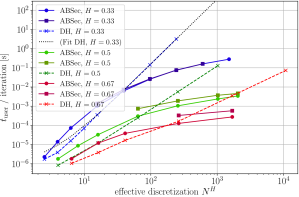
Figure 6: Average user time required to find first-passage time in a grid of effective discretization precision $2^{-LH}$. The dashed lines indicate user time for Davies-Harte method, solid lines for the adaptive bisection method. The three different colours indicate $H=0.33,0.5,0.67$. Simulations were run $10^{4}$ times for $\varepsilon^{\prime}=10^{-9}$ and for two different initial subgrid sizes ($\Lambda^{4}$ circles; $\Lambda^{8}$ squares).

We measure the average user time per generated first-passage time, using either DH or ABSec. To render different Hurst-values and algorithms comparable, we plot the user time versus the inverse of the effective discretization error, which scales as $N^{H}$ for DH and $2^{LH}$ for ABSec. It describes how well the fBm-path is resolved numerically, taking into account the fluctuation scaling for different Hurst-parameters.

Since at the beginning of the ABSec procedure inverse correlation matrices are tabulated (cf. section II.3.4), we measured the run time for $10^{4}$ iterations, in order to render the initial overhead irrelevant.

Fig. 6 shows the result of the benchmarking. For small effective system sizes, ABSec performs slower than DH, which is due to the relatively complex overhead of bisections. For (effective) system sizes of $N\gtrsim 10^{\frac{2}{H}}$ the ABSec algorithm gains an increasing and significant advantage since its run time only grows sublinearly.

To estimate performance time, we observe that for values of $H\geq 0.33$, the number of additional gridpoints $M$ grows linearly in effective system size (cf. Fig. 5) throughout the entire observed range. Based on our empirical findings, we propose a linear relation $M\sim L=\log_{2}(N_{\rm eff})$, which implies, cf. Eq. (5), an overall computational complexity of

$${\cal C}^{\rm ABSec}(N_{\rm eff})={\cal O}\left(\left(\ln N_{\rm eff}\right)^{3}\right)\ ,\qquad H\gtrsim\frac{1}{3}\ ,$$ (35)

since $M\gg 2^{g}$. This estimate is corroborated by Fig. 8, where the scaling of user time with system size agrees with our estimate of $\log(N_{\rm eff})^{3}$ for sufficiently large system sizes. The linear relation between the number of bisections $M$ and the logarithmic system size $L$, however, does not extend to smaller values of $H$, where Fig. 5 indicates super-linear growth. Still, testing the ABSec routine at $H=0.25$ for an effective system size of $N_{\rm eff}=2^{42}$ gave an average user time of $6.2s$ and was about $300000$ faster than an extrapolation of the user time for DH at the same system size. This shows that for all practical purposes, ABSec remains a much faster algorithm even at parameters where estimate (35) seems to no longer hold.

For $H=0.33$, due to memory limitations, DH is unable to generate paths larger than $N=2^{24}$, where ABSec is already about 40 times faster. Since ABSec is also more memory-efficient (see next section), we can generate grids of size up to $2^{32}$ for which, if we interpolate the growth of DH, we find that ABSec is 5500 times faster than DH for these parameters. For $H>\frac{1}{2}$, the advantage is less pronounced, and at a comparable discretization precision, the algorithm is “only” 40-50 times faster at $H=0.67$.

Performance also depends on the initial grid size. In Figs. 6 and 7, we compare run times for two different initial grids, $\Lambda^{4}$ and $\Lambda^{8}$. For larger initial grid sizes, the algorithm is slower since more points need to be generated initially. An increase in initial grid size leads to a decrease of 15% (for $H=0.33$) in the average number of bisections. This is approximately outweighed by the time DH takes to generate a path on $\Lambda^{8}$ (cf. Fig. 6).

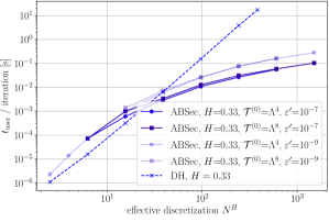
Figure 7: User time for ABSec compared to DH for two different initial grid sizes and two different values of error tolerance $\varepsilon^{\prime}$. For a hundred times higher error tolerance, user time increase by up to $60\%$.

The run time increases only slowly for a smaller error tolerance. In Fig. 7, we show how user time decreases when changing $\epsilon^{\prime}$ from $\varepsilon^{\prime}=10^{-9}$ to $\varepsilon^{\prime}=10^{-7}$. For an effective precision of $2^{\frac{32}{3}}$, user time increases by roughly 60 %. Since error rates grow linearly with $\varepsilon^{\prime}$ (see Fig. 3), we conclude that for an error rate 100 times lower one only needs to invest 60% more user time.

All together, these observations show that the algorithm behaves in a controlled manner for varying error tolerances and initial grid sizes. Depending on the number of iterations, and the quality of the data desired, choosing $g$ (initial grid size), $L$ (desired precision), and $\varepsilon^{\prime}$ (error tolerance level) accordingly leads to an algorithm that performs up to 5000 times faster than DH at $H=0.33$, that was hitherto very hard to access with high precision. The algorithm should be tested more for $H=0.25$, where it allows one to reach a precision unimaginable by DH.

Figure 8: $(t_{\rm user}/{\rm iteration})^{1/3}$ plotted versus effective discretization $N^{H}$ for various values of $H$ (blue $H=0.33$, green $H=0.5$, red $H=0.67$, cf. Fig. 6). They corroborate the estimate of ${\cal C}^{\rm ABSec}\sim\log(N_{\rm eff})^{3}$. Straight lines indicate fits of the form $a\log(N)+b$. The inset shows the ratio between data points and the fit.

III.6 Memory requirements

As a final benchmark of our algorithm, we consider memory usage. The latter is defined by the resident set size of the process, as measured by getrusage. When using DH, the full grid needs to be saved, and in doing so memory usage scales like $N$. Fig. 9 shows memory usage for both DH and ABSec when performed for different effective discretization precisions and initial grid sizes. It shows that for large system sizes, ABSec gains a growing and significant advantage. To generate a path of $2^{28}$ lattice points in double precision via DH, one requires 10 GB working memory, whereas ABSec uses between 20 and 80 MB, depending on the initial grid size. This represents an improvement by a factor of 125 to 500. This is due to the fact that only the initial grid which scales as $\mathcal{O}(2^{g})$, the additional gridpoints of order $\mathcal{O}(M)$ and a correlation matrix, scaling as $\mathcal{O}(2^{g}+M)^{2}$, need to be stored. As implemented, additional memory is needed for the catalogue of inverse correlation matrices (cf. Eq. (14)) which occupies memory of order $\mathcal{O}(2^{3g})$, so including the catalogue overall memory space grows like $2^{3g}+(2^{g}+M)^{2}$. Since we can assume that $2^{g}\ll M$, the necessary memory grows with order $M^{2}$. For values of $H\gtrsim\frac{1}{3}$, we empirically found that $M\sim\log(N_{\rm eff})$, such that in that parameter range we estimate memory to grow with

$${\cal M}^{\rm ABSec}(N_{\rm eff})=\mathcal{O}\left(\log(N_{\rm eff})^{2}\right),\qquad H\gtrsim\frac{1}{3}\ .$$ (36)

This advantage is again due to $M\ll 2^{L}$, i.e. using the fact that the first-passage time can be found to equal precision with much less grid points.

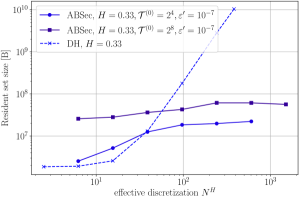
Figure 9: Memory usage for DH and ABSec for two different initial subgrid sizes. DH scales linearly in $N$, while ABSec grows only slowly (see text for estimate). For system of size $N_{\rm eff}=2^{28}$, ABSec needs only $10^{-2}$ to $10^{-3}$ of the memory for DH. For larger systems or smaller $H$, the advantage of ABSec is even bigger. Measurements were taken after $10^{4}$ iterations.

III.7 Floating point precision

Currently, our implementation uses the 64-bit double type. Since the variance of a bridge-point is calculated from the subtraction of quantities of $\mathcal{O}(1)$ (cf. Eq. (30)) whose difference can be as small as $\mathcal{O}(2^{-LH})$, the subtraction suffers from the finite floating-point precision when $L$ is too large, as is demonstrated in Fig. 10 (cf. caption for details). This leads to $L_{\rm max}\simeq 10.5/H$, or $N\simeq 2\times 10^{\frac{3}{H}}$.

Figure 10: Ratio between sampled variance and no-neighbour-estimate of variance (cf. Eq. (17)) of an inserted midpoint $X_{m}$ versus the level of the bisected bridge. For $H=0.5$ (green), the ratio equals 1, as BM is Markovian. For $H\neq 0.5$, the variance fluctuates, as shown by the error bars for one standard deviation. Numerical errors due to a loss of floating point precision become relevant around $L_{\rm max}\simeq 11/H$. ABSec was used with an initial grid $\Lambda^{8}$ and $\varepsilon^{\prime}=10^{-9}$.

III.8 Discussion

In this section we illuminated several aspects of our algorithm that show how it is capable of generating first-passage times with high numerical precision using several orders of magnitude less CPU time and memory as compared to DH. We chose to compare ABSec to DH because the latter is widely spread in simulating first-passage times of fBm (see e.g. Guerin2016 ; Levernier2018 ), and since it is the fastest known exact generator of fBm. Since our method is also exact (the statistics of the grid generated is bias-free), we think of DH as the natural benchmark. There are related approximative algorithms like the random midpoint displacement algorithm $R_{\ell,r}$ that also inserts midpoints, only taking into account the $\ell$ left and $r$ right nearest neighbours Norros2004 . This neglects long-range correlations between small increments at $t_{1},t_{2}$ which even for $t_{1}\ll t_{2}$ are correlated algebraically via $(t_{1}-t_{2})^{-1}+\mathcal{O}\left((H-\frac{1}{2})^{2}\right)$ (for $H\neq\frac{1}{2}$). The ABSec algorithm uses the full inverse correlation matrix of all points generated and is therefore closely related to exact procedures like DH.

Supported by our experiments, we are able to control both vertical and horizontal errors at the scale of inherent errors of a Monte Carlo simulation. In practice, the limiting factors are not systematical errors of the algorithm but floating point imprecisions stemming from the matrix inversion.

The phone-book test used to asses the error rate does not take into account issues of precision when drawing new midpoints, which are copied from a pre-generated grid. Since this is an implementation-dependent grid, we decided to only use the phone-book test since the errors caused in that procedure are the ones inherent to the algorithm itself. An implementation with a higher-precision floating-point unit seems highly desirable.

IV Summary

When simulating first-passage times, or any other non-local observable, of fractional Brownian Motion, the large fluctuations for $H<\frac{1}{2}$ require the grid to have a very high resolution for the same quality of data as for $H\geq\frac{1}{2}$. Generating a fine grid is particularly expensive, both in memory and time. The algorithm proposed here refines the grid only where it is likely to impact the first-passage event. To give rigorous notion to that idea, we developed a precise criterion for when and where the grid should be refined. The new mid-points are then sampled exactly. Comparing it to the fastest known exact sampler, the Davies-Harte algorithm, we find that our implementation of the algorithm is 5000 times faster and uses 1000 times less memory when applied to $H=0.33$ at $N_{\rm eff}=2^{32}$, due to the fact that only roughly $0.1\%$ of the full grid is needed to determine the first-passage event. Our algorithm works with a probabilistic approximation, and the error rate can be bounded by $10^{-6}$ or even $10^{-8}$. This should be sufficient for most Monte Carlo experiments and be in the order of numerical (algorithm-independent) errors.

We have successfully used the algorithm to validate the analytic results for the first-passage time in Ref. ArutkinWalterWiese2019 . There we used 2.5 CPU years at precision $N=2^{28}$. With DH we would have had to reduce the precision to $N=2^{24}$, which still would have taken 75 CPU years.

Finally, the concepts presented here can be used for other observables and other Gaussian processes. We hope that our algorithm contributes to confirming theoretical predictions on extreme events in Gaussian processes that where hitherto numerically inaccessible at the required precision.

Appendix A Derivation of the critical strip length

In this section we derive the width of the critical strip which was introduced in Sec. II.3.5. The critical strip refers to the distance between a fBm-bridge of size $\delta t=2^{-\ell}$ and the threshold $m$, below which the midpoint of the bridge may surpass the threshold with probability larger than $\varepsilon$. We ignore any other grid points beyond the two fixed bridge points. By translational invariance, we set $X_{0}=0$, and $X_{\delta t}=a$ ($a\in\mathbb{R})$. The problem is then equivalently stated as

$$P(X^{\rm B}_{\delta t/2}>c(\varepsilon))=\varepsilon,$$ (37)

where $X^{\rm B}_{t}$ is the fBm-bridge process conditioned on $X_{0},X_{\delta t}$. Following the derivation in DelormeWiese2016b , the law of the fBm-bridge is itself a Gaussian process with first and second moment,

$$\left\langle X^{\rm B}_{t}\right\rangle =\frac{\left\langle X_{t}\delta(X_{\delta t}-a)\right\rangle}{\left\langle\delta(X_{\delta t}-a)\right\rangle}\ ,$$ (38)

$$\left\langle X^{\rm B}_{s}X^{\rm B}_{t}\right\rangle =\frac{\left\langle X_{s}X_{t}\delta(X_{\delta t}-a)\right\rangle}{\left\langle\delta(X_{\delta t}-a)\right\rangle}\ ,$$ (39)

where on the right-hand-side the averages are over free fBm paths. As shown in Resf. DelormeWiese2016b , Eqs. (8) and (9), the averages are

$$\left\langle X^{\rm B}_{t}\right\rangle =a\frac{C(t,\delta t)}{C(\delta t,\delta t)}$$ (40)

$$\left\langle X^{\rm B}_{s}X^{\rm B}_{t}\right\rangle^{\rm c} =C(s,t)-\frac{C(s,\delta t)C(t,\delta t)}{C(\delta t,\delta t)}\ ,$$ (41)

where $C(s,t)$ is the correlation function of Eq. (3). Since we are only interested in the midpoint with $s=t=\delta t/2$, this yields

$$\mu=\left\langle X_{\delta t/2}^{\rm B}\right\rangle =\frac{a}{2}\ ,$$ (42)

$$\sigma=\left\langle(X^{\rm B}_{\delta t/2})^{2}\right\rangle^{\rm c} =\left(2^{1-2H}-\frac{1}{2}\right)\left(\delta t\right)^{2H}\ .$$ (43)

This determines the normal distribution of the midpoint and by translational invariance proves the values used in Sec. II.3.5.

Appendix B How to generate an additional random midpoint

We derive the conditional law of an additional randomly generated midpoint for an arbitrary Gaussian processes as given in Eqs. (25)–(26). Let $\mathcal{T}^{N}=t_{1},\cdots,t_{N}$ and $\mathcal{X}^{N}=X_{t_{1}},\cdots,X_{t_{N}}$ be given, and denote the point to be inserted by $t_{N+1}$ and $X_{t_{N+1}}$ (the times are not ordered). For ease of notation, we write $X_{i}=X_{t_{i}}$. As a Gaussian process, the vector $\vec{X}=(X_{1},\cdots,X_{N},X_{{N+1}})^{T}$ is a normal random variable with mean zero and covariance matrix

$$\left\langle\vec{X}\vec{X}^{T}\right\rangle=C(t_{i},t_{j})=:C(N+1)\ ,\quad 1\leq i,j\leq N\ .$$ (44)

It has a symmetric inverse correlation matrix $C^{-1}_{i,j}$. Its probability law is therefore given by

$$P(\vec{X})=\frac{\exp\left(-\frac{1}{2}\sum_{i,j=1}^{N+1}X_{i}C^{-1}_{i,j}X_{j}\right)}{\sqrt{(2\pi)^{N+1}\det(C)}}\ .$$ (45)

Since $X_{1},\cdots,X_{N}$ are fixed, $X_{{N+1}}$ conditioned on ${\cal X}^{N}$ follows the marginal distribution

$$P(X_{{N+1}}|\mathcal{X}^{N})$$

$$=\frac{\exp\left(-\frac{1}{2}X_{N+1}^{2}C^{-1}_{N+1,N+1}-\sum_{j=1}^{N}X_{j}C^{-1}_{N+1,j}X_{N+1}\right)}{{\sqrt{2\pi/C^{-1}_{N+1,N+1}}}}\ .$$ (46)

Note that the normalizing factor in Eq. (45) has cancelled, since Eq. (46) is a conditional average. This is a Gaussian distribution

$$P(X_{{N+1}}|\mathcal{X}^{N})=\frac{\exp\left(-\frac{\sigma^{2}}{2}\left(X_{N+1}-\mu\right)^{2}\right)}{\sqrt{2\pi}\sigma}\ ,$$ (47)

with variance

$$\sigma^{2}=\frac{1}{C^{-1}_{N+1,N+1}}\ ,$$ (48)

and mean

$$\mu=-\sum_{j=1}^{N}X_{j}\frac{C^{-1}_{N+1,j}}{C^{-1}_{N+1,N+1}}.$$ (49)

The mean can be seen as an average of the $X_{j}$ with weight ${C^{-1}_{N+1,j}}/{C^{-1}_{N+1,N+1}}$.

Appendix C Derivation of the enlarged correlation matrix

In this section, we derive the algorithm to promote inverse correlation matrices as given in Eqs. (27)–(32). Assuming that $C(N)$ and $C^{-1}(N)$ are known, the aim is to find $C(N+1)$ and $C^{-1}(N+1)$ in as little as possible computational steps. The starting point is the observation that $C(N+1)$ contains $C(N)$ as block matrix and is only augmented by a row and identical column,

$$C(N+1)=\begin{pmatrix}C(N)&\vline&\vec{\gamma}\\ \hline\cr\vec{\gamma}^{T}&\vline&\left\langle X_{N+1}^{2}\right\rangle\end{pmatrix}$$ (50)

where $\vec{\gamma}$ is defined in Eq. (27) and $\left\langle X_{N+1}^{2}\right\rangle=2t_{N+1}^{2H}$ in the case of fBm, but is intentionally left general. For the more difficult part, the inversion, we assume that the inverse correlation matrix is of the form

$$C^{-1}(N+1)=\begin{pmatrix}A(N)&\vline&\vec{b}\\ \hline\cr\vec{b}^{T}&\vline&c\end{pmatrix}$$ (51)

for some arbitrary (symmetric) matrix $A$, vector $\vec{b}$ and number $c$. Multiplying matrices (50) and (51) results in

$$CC^{-1} =\begin{pmatrix}C(N)A(N)+\gamma\otimes\vec{b}^{T}&\vline&C(N)\vec{b}+c\vec{\gamma}\\ \hline\cr(C(N)\vec{b}+c\vec{\gamma})^{T}&\vline&\vec{b}^{T}\vec{\gamma}+c\left\langle X^{2}_{N+1}\right\rangle\end{pmatrix}$$

$$\stackrel{{\scriptstyle!}}{{=}}\mathbf{1}_{N+1}\ ,$$ (52)

such that one obtains the system of equations

$$C(N)A(N)+\vec{\gamma}\otimes\vec{b}^{T} =\mathbf{1}_{N}\ ,$$ (53)

$$C(N)\vec{b}+c\vec{\gamma} =\vec{0}\ ,$$ (54)

$$\vec{b}^{T}\gamma+c\left\langle X^{2}_{N+1}\right\rangle =1\ .$$ (55)

This is solved by

$$A(N) =C^{-1}(N)+\frac{C^{-1}(N)\vec{\gamma}\otimes\vec{\gamma}^{T}C^{-1}(N)}{\left\langle X_{N+1}^{2}\right\rangle-\vec{\gamma}^{T}C^{-1}(N)\vec{\gamma}}\ ,$$ (56)

$$\vec{b} =-\frac{C^{-1}(N)\vec{\gamma}}{\left\langle X_{N+1}^{2}\right\rangle-\vec{\gamma}^{T}C^{-1}(N)\vec{\gamma}}\ ,$$ (57)

$$c =\frac{1}{\left\langle X^{2}_{N+1}\right\rangle-\vec{\gamma}^{T}C^{-1}(N)\vec{\gamma}}\ .$$ (58)

Defining $\vec{g}$ as in Eq. (28) and $\sigma^{2}$ as in Eq. (30), one arrives at the inverse matrix (32).

References

- (1) S. Redner, A Guide to First-Passage Processes, Cambridge University Press, 2001.
- (2) R. Metzler, G. Oshanin and S. Redner, First-Passage Phenomena and Their Applications, World Scientifc, 2014.
- (3) P. Hänggi, P. Talkner and M. Borkovec, Reaction-rate theory: fifty years after Kramers, Rev. Mod. Phys. 62 (1990) 251–341.
- (4) A. Godec and R. Metzler, First passage time distribution in heterogeneity controlled kinetics: going beyond the mean first passage time, Scientific Reports 6 (2016) 20349.
- (5) L.P. Sanders and T. Ambjörnsson, First passage times for a tracer particle in single file diffusion and fractional Brownian motion, J. Chem. Phys. 136 (2012) 175103.
- (6) T. Guérin, N. Levernier, O. Bénichou and R. Voituriez, Mean first-passage times of non-markovian random walkers in confinement, Nature 534 (2016) 356–359.
- (7) N. Levernier, O. Bénichou, T. Guérin and R. Voituriez, Universal first-passage statistics in aging media, Phys. Rev. E 98 (2018) 022125.
- (8) K.J. Wiese, First passage in an interval for fractional Brownian motion, Phys. Rev. E 99 (2018) 032106, arXiv:1807.08807.
- (9) M. Arutkin, B. Walter and K.J. Wiese, Fractional Brownian motion with drift: Theory and numerical validation, (2019), arXiv:1908.10801.
- (10) B.B. Mandelbrot and J.W. Van Ness, Fractional Brownian motions, fractional noises and applications, SIAM Review 10 (1968) 422–437.
- (11) K.J. Wiese, S.N. Majumdar and A. Rosso, Perturbation theory for fractional Brownian motion in presence of absorbing boundaries, Phys. Rev. E 83 (2011) 061141, arXiv:1011.4807.
- (12) M. Delorme and K.J. Wiese, Maximum of a fractional Brownian motion: Analytic results from perturbation theory, Phys. Rev. Lett. 115 (2015) 210601, arXiv:1507.06238.
- (13) T. Sadhu, M. Delorme and K.J. Wiese, Generalized arcsine laws for fractional Brownian motion, Phys. Rev. Lett. 120 (2018) 040603, arXiv:1706.01675.
- (14) R.B. Davies and D.S. Harte, Tests for Hurst effect, Biometrika 74 (1987) 95–101.
- (15) D. M. Ceperley, Path integrals in the theory of condensed helium, Rev. Mod. Phys. 67 (1995) 279–355.
- (16) M. Sprik, M. L. Klein and D. Chandler, Staging: A sampling technique for the Monte Carlo evaluation of path integrals, Phys. Rev. B 31 (1985) 4234–4244.
- (17) A. Fournier, D. Fussell and L. Carpenter, Computer rendering of stochastic models, Communications of the ACM 25 (1982) 371–384.
- (18) I. Norros, P. Mannersalo and J. L. Wang, Simulation of fractional brownian motion with conditionalized random midpoint displacement, Advances in Performance Analysis 2 (1999) 77–101.
- (19) A.B. Dieker, Simulation of fractional Brownian motion, PhD thesis, University of Twente, 2004.
- (20) P.F. Craigmile, Simulating a class of stationary gaussian processes using the Davies-Harte algorithm, with application to long memory processes, Journal of Time Series Analysis 24 (2003) 505–511.
- (21) D. Krapf, N. Lukat, E. Marinari, R. Metzler, G. Oshanin, C. Selhuber-Unkel, A. Squarcini, L. Stadler, M. Weiss and X. Xu, Spectral content of a single non-brownian trajectory, Phys. Rev. X 9 (2019) 011019.
- (22) B. Walter and K.J. Wiese, Monte Carlo sampler of first-passage times for fractional Brownian motion using adaptive bisections: Source code, hal-02270046 (2019). Also available at github.
- (23) V.I. Piterbarg, Twenty Lectures about Gaussian Processes, Atlantic Financial Press, 2015.
- (24) G.H. Weiss and R.J. Rubin, The theory of ordered spans of unrestricted random walks, J. Stat. Phys 14 (1976) 333–350.
- (25) G.H. Weiss, E.A. DiMarzio and R.J. Gaylord, First passage time densities for random walk spans, J. Stat. Phys. 42 (1986) 567–572.
- (26) V. Palleschi and M.R. Torquati, Mean first-passage time for random-walk span: Comparison between theory and numerical experiment, Phys. Rev. A 40 (1989) 4685–4689.
- (27) K.J. Wiese, Span observables - “When is a foraging rabbit no longer hungry?”, (2019), arXiv:1903.06036.
- (28) E. Anderson et al., LAPACK Users’ Guide, Society for Industrial and Applied Mathematics, Philadelphia, PA, third edition, 1999.
- (29) M. Galassi et al., GNU Scientific Library Reference Manual. 2 edition.
- (30) M. Frigo, A fast Fourier transform compiler, in Proceedings of the ACM SIGPLAN 1999 Conference on Programming Language Design and Implementation, PLDI ’99, pages 169–180, ACM, New York, NY, USA, 1999.
- (31) BLAS (Basic Linear Algebra Subprograms), www.netlib.org/blas.
- (32) M. Delorme and K.J. Wiese, Extreme-value statistics of fractional Brownian motion bridges, Phys. Rev. E 94 (2016) 052105, arXiv:1605.04132.