Circumcentered methods induced by isometries

Abstract

Motivated by the circumcentered Douglas–Rachford method recently introduced by Behling, Bello Cruz and Santos to accelerate the Douglas–Rachford method, we study the properness of the circumcenter mapping and the circumcenter method induced by isometries. Applying the demiclosedness principle for circumcenter mappings, we present weak convergence results for circumcentered isometry methods, which include the Douglas–Rachford method (DRM) and circumcentered reflection methods as special instances. We provide sufficient conditions for the linear convergence of circumcentered isometry/reflection methods. We explore the convergence rate of circumcentered reflection methods by considering the required number of iterations and as well as run time as our performance measures. Performance profiles on circumcentered reflection methods, DRM and method of alternating projections for finding the best approximation to the intersection of linear subspaces are presented.

2020 Mathematics Subject Classification: Primary 47H09, 65K10; Secondary 41A50, 65K05, 90C25.

Keywords: circumcenter mapping, isometry, reflector, best approximation problem, linear convergence, circumcentered reflection method, circumcentered isometry method, Douglas–Rachford method.

1 Introduction

Throughout this paper, we assume that

$$\mathcal{H}$$ is a real Hilbert space

with inner product $\langle\cdot,\cdot\rangle$ and induced norm $\|\cdot\|$. Denote the set of all nonempty subsets of $\mathcal{H}$ containing finitely many elements by $\mathcal{P}(\mathcal{H})$. Given $K\in\mathcal{P}(\mathcal{H})$, the circumcenter of $K$ is defined as either empty set or the unique point $CC{(K)}$ such that $CC{(K)}\in\operatorname{aff}\,(K)$ and $CC{(K)}$ is equidistant from all points in $K$, see [4, Proposition 3.3].

Let $m\in\mathbb{N}\smallsetminus\{0\}$, and let $T_{1},\ldots,T_{m-1},T_{m}$ be operators from $\mathcal{H}$ to $\mathcal{H}$. Assume

$$\mathcal{S}=\{T_{1},\ldots,T_{m-1},T_{m}\}\quad\text{with}\quad\bigcap^{m}_{j=1}\operatorname{Fix}T_{j}\neq\varnothing.$$

The associated set-valued operator $\mathcal{S}:\mathcal{H}\rightarrow\mathcal{P}(\mathcal{H})$ is defined by

$$(\forall x\in\mathcal{H})\quad\mathcal{S}(x):=\{T_{1}x,\ldots,T_{m-1}x,T_{m}x\}.$$

The circumcenter mapping $CC_{\mathcal{S}}$ induced by $\mathcal{S}$ is defined by the composition of $CC{}$ and $\mathcal{S}$, that is $(\forall x\in\mathcal{H})$ $CC_{\mathcal{S}}(x)=CC{}\left(\mathcal{S}(x)\right)$. If $CC_{\mathcal{S}}$ is proper, i.e., $(\forall x\in\mathcal{H})$, $CC_{\mathcal{S}}x\in\mathcal{H}$, then we are able to define the circumcenter methods induced by $\mathcal{S}$ as

$$x_{0}=x,~{}\mbox{and}~{}x_{k}=CC_{\mathcal{S}}(x_{k-1})=CC_{\mathcal{S}}^{k}x,~{}\mbox{where}~{}k=1,2,\ldots.$$

Motivated by Behling, Bello Cruz and Santos [7], we worked on circumcenters of finite set in Hilbert space in [4] and on the properness of circumcenter mappings in [5]. For other recent developments on circumcentered isometry methods, see also [9], [10], [16] and [6]. In this paper, we study the properness of the circumcenter mapping induced by isometries, and the circumcenter methods induced by isometries. Isometry includes reflector associated with closed affine subspaces. We provide convergence or even linear convergence results of the circumcentered isometry methods. In particular, for circumcentered reflection methods, we also offer some applications and evaluate their linear convergence rate by comparing them with two classical algorithms, namely, the Douglas-Rachford method (DRM) and the method of alternating projections (MAP).

More precisely, our main results are the following:

• Theorem 3.3 provides the properness of the circumcenter mapping induced by isometries.

• Theorem 4.7 presents a sufficient condition for the weak convergence of circumcentered isometry methods.

• Theorems 4.14 and 4.15 present sufficient conditions for the linear convergence of circumcentered isometry methods in Hilbert space and $\mathbb{R}^{n}$, respectively.

• Proposition 5.18 takes advantage of the linear convergence of DRM to build the linear convergence of other circumcentered reflection methods.

Theorem 3.3 extends [5, Theorem 4.3] from reflectors to isometries. Based on the demiclosedness principle for circumcenter mappings built in [5, Theorem 3.20], we obtain the Theorem 4.7, which implies the weak convergence of the DRM and the circumcentered reflection method, the main actor in [8]. Motivated by the role played by the Douglas–Rachford operator in the proof of [7, Theorem 1], we establish Theorem 4.14 and Proposition 5.18. As a corollary of Proposition 5.18, we observe that Proposition 5.19 yields [7, Theorem 1]. Motivated by the role that the firmly nonexpansive operator $A$ played in [8, Theorem 3.3] to deduce the linear convergence of circumcentered reflection method in $\mathbb{R}^{n}$, we obtain Proposition 2.10 and Theorem 4.15(ii). Theorem 4.15(ii) says that some $\alpha$-averaged operators can be applied to construct linear convergent methods, which imply the linear convergence of the circumcentered isometry methods. As applications of Theorem 4.15(ii), Propositions 5.10, 5.14 and 5.15 display particular classes of circumcentered reflection methods being linearly convergent.

The rest of the paper is organized as follows. In Section 2, we present various basic results for subsequent use. Our main theory results start at Section 3. Some results in [5, Section 4.1] are generalized in Section 3.1 to deduce the properness of the circumcenter mapping induced by isometries. Thanks to the properness, we are able to generate the circumcentered isometry methods in Section 4. In Section 4.2, we focus on exploring sufficient conditions for the (weak, strong and linear) convergence of the circumcentered isometry methods. In Sections 5 and 6, we consider the circumcentered reflection methods. In Section 5, first, we display some particular linearly convergent circumcentered reflection methods. Then the circumcentered reflection methods are used to accelerate the DRM, which is then used to find best approximation onto the intersection of finitely many linear subspaces. Finally, in Section 6, in order to evaluate the rate of linear convergence of the circumcentered reflection methods, we use performance profile with performance measures on both required number of iterations and run time to compare four circumcentered reflection methods with DRM and MAP for solving the best approximation problems associated with two linear subspaces with Friedrichs angle taken in certain ranges.

We now turn to notation. Let $C$ be a nonempty subset of $\mathcal{H}$. Denote the cardinality of $C$ by $\operatorname{card}(C)$. The intersection of all the linear subspaces of $\mathcal{H}$ containing $C$ is called the span of $C$, and is denoted by ${\operatorname{span}\,}C$; its closure is the smallest closed linear subspace of $\mathcal{H}$ containing $C$ and it is denoted by $\overline{{\operatorname{span}\,}}~{}C$. $C$ is an affine subspace of $\mathcal{H}$ if $C\neq\varnothing$ and $(\forall\rho\in\mathbb{R})$ $\rho C+(1-\rho)C=C$; moreover, the smallest affine subspace containing $C$ is the affine hull of $C$, denoted $\operatorname{aff}\,C$. An affine subspace $U$ is said to be parallel to an affine subspace $M$ if $U=M+a$ for some $a\in\mathcal{H}$. Every affine subspace $U$ is parallel to a unique linear subspace $L$, which is given by $(\forall y\in U)$ $L:=U-y=U-U$. For every affine subspace $U$, we denote the linear subspace parallel to $U$ by $\operatorname{par}U$. The orthogonal complement of $C$ is the set $C^{\perp}=\{x\in\mathcal{H}~{}|~{}\langle x,y\rangle=0~{}\text{for all}~{}y\in C\}.$ The best approximation operator (or projector) onto $C$ is denoted by $\operatorname{P}_{C}$ while $\operatorname{R}_{C}:=2\operatorname{P}_{C}-\operatorname{Id}$ is the reflector associated with $C$. For two subsets $A$, $B$ of $\mathcal{H}$, the distance $\operatorname{d}(A,B)$ is $\inf\lVert A-B\rVert$. A sequence $(x_{k})_{k\in\mathbb{N}}$ in $\mathcal{H}$ converges weakly to a point $x\in\mathcal{H}$ if, for every $u\in\mathcal{H}$, $\langle x_{k},u\rangle\rightarrow\langle x,u\rangle$; in symbols, $x_{k}{\;\operatorname{\rightharpoonup}\;}x$. Let $T:\mathcal{H}\rightarrow\mathcal{H}$ be an operator. The set of fixed points of the operator $T$ is denoted by $\operatorname{Fix}T$, i.e., $\operatorname{Fix}T:=\{x\in\mathcal{H}~{}|~{}Tx=x\}$. $T$ is asymptotically regular if for each $x\in\mathcal{H}$, $T^{k}x-T^{k+1}x\to 0$. For other notation not explicitly defined here, we refer the reader to [3].

2 Auxiliary results

This section contains several results that will be useful later.

2.1 Projections

Fact 2.1

[3, Proposition 29.1] Let $C$ be a nonempty closed convex subset of $\mathcal{H}$, and let $x\in\mathcal{H}$. Set $D:=z+C$, where $z\in\mathcal{H}$. Then $\operatorname{P}_{D}x=z+\operatorname{P}_{C}(x-z)$.

Fact 2.2

[11, Theorems 5.8 and 5.13] Let $M$ be a closed linear subspace of $\mathcal{H}$. Then:

1. $x=\operatorname{P}_{M}x+\operatorname{P}_{M^{\perp}}x$ for each $x\in\mathcal{H}$. Briefly, $\operatorname{Id}=\operatorname{P}_{M}+\operatorname{P}_{M^{\perp}}$.

2. $M^{\perp}=\{x\in\mathcal{H}~{}|~{}\operatorname{P}_{M}(x)=0\}$ and $M=\{x\in\mathcal{H}~{}|~{}\operatorname{P}_{M^{\perp}}(x)=0\}=\{x\in\mathcal{H}~{}|~{}\operatorname{P}_{M}(x)=x\}$.

Fact 2.3

[5, Proposition 2.10] Let $C$ be a closed affine subspace of $\mathcal{H}$. Then the following hold:

1. The projector $\operatorname{P}_{C}$ and the reflector $\operatorname{R}_{C}$ are affine operators.

2. $(\forall x\in\mathcal{H})$ $(\forall v\in C)$ $\lVert x-\operatorname{P}_{C}x\rVert^{2}+\lVert\operatorname{P}_{C}x-v\rVert^{2}=\lVert x-v\rVert^{2}$.

3. $(\forall x\in\mathcal{H})$ $(\forall y\in\mathcal{H})$ $\lVert x-y\rVert=\lVert\operatorname{R}_{C}x-\operatorname{R}_{C}y\rVert$.

Lemma 2.4

Let $M:=\operatorname{aff}\,\{x,x_{1},\ldots,x_{n}\}\subseteq\mathcal{H}$, where $x_{1}-x,\ldots,x_{n}-x$ are linearly independent. Then for every $y\in\mathcal{H}$,

$$\operatorname{P}_{M}(y)=x+\sum^{n}_{i=1}\langle y-x,e_{i}\rangle e_{i},$$

where $(\forall i\in\{1,\ldots,n\})\quad e_{i}=\frac{x_{i}-x-\sum^{i-1}_{j=1}\langle x_{i}-x,e_{j}\rangle e_{j}}{\lVert x_{i}-x-\sum^{i-1}_{j=1}\langle x_{i}-x,e_{j}\rangle e_{j}\rVert}$.

Proof.

Since $x_{1}-x,\ldots,x_{n}-x$ are linearly independent, by the Gram-Schmidt orthogonalization process [17, page 309], let $\big{(}\forall i\in\{1,\ldots,n\}\big{)}$ $e_{i}:=\frac{x_{i}-x-\sum^{i-1}_{j=1}\langle x_{i}-x,e_{j}\rangle e_{j}}{\lVert x_{i}-x-\sum^{i-1}_{j=1}\langle x_{i}-x,e_{j}\rangle e_{j}\rVert}$, then $e_{1},\ldots,e_{n}$ are orthonormal. Moreover

$${\operatorname{span}\,}\{e_{1},\ldots,e_{n}\}={\operatorname{span}\,}\{x_{1}-x,\ldots,x_{n}-x\}:=L.$$

Since $M=x+L$, thus by Fact 2.1, we know $\operatorname{P}_{M}(y)=x+\operatorname{P}_{L}(y-x).$ By [3, Proposition 29.15], we obtain that for every $z\in\mathcal{H}$, $\operatorname{P}_{L}(z)=\sum^{n}_{i=1}\langle z,e_{i}\rangle e_{i},$ where $(\forall i\in\{1,\ldots,n\})$ $e_{i}=\frac{x_{i}-x-\sum^{i-1}_{j=1}\langle x_{i}-x,e_{j}\rangle e_{j}}{\lVert x_{i}-x-\sum^{i-1}_{j=1}\langle x_{i}-x,e_{j}\rangle e_{j}\rVert}$. ∎

2.2 Firmly nonexpansive mappings

Definition 2.5

[3, Definition 4.1] Let $D$ be a nonempty subset of $\mathcal{H}$ and let $T:D\rightarrow\mathcal{H}$. Then $T$ is

1. firmly nonexpansive if

   $$(\forall x,y\in D)\quad\lVert Tx-Ty\rVert^{2}+\lVert(\operatorname{Id}-T)x-(\operatorname{Id}-T)y\rVert^{2}\leq\lVert x-y\rVert^{2};$$

2. nonexpansive if it is Lipschitz continuous with constant 1, i.e.,

   $$(\forall x,y\in D)\quad\lVert Tx-Ty\rVert\leq\lVert x-y\rVert;$$

3. firmly quasinonexpansive if

   $$(\forall x\in D)\quad(\forall y\in\operatorname{Fix}T)\quad\lVert Tx-y\rVert^{2}+\lVert Tx-x\rVert^{2}\leq\lVert x-y\rVert^{2};$$

4. quasinonexpansive if

   $$(\forall x\in D)\quad(\forall y\in\operatorname{Fix}T)\quad\lVert Tx-y\rVert\leq\lVert x-y\rVert.$$

Fact 2.6

[3, Corollary 4.24] Let $D$ be a nonempty closed convex subset of $\mathcal{H}$ and let $T:D\to\mathcal{H}$ be nonexpansive. Then $\operatorname{Fix}T$ is closed and convex.

Definition 2.7

[3, Definition 4.33] Let $D$ be a nonempty subset of $\mathcal{H}$, let $T:D\rightarrow\mathcal{H}$ be nonexpansive, and let $\alpha\in\,]0,1[\,$. Then $T$ is averaged with constant $\alpha$, or $\alpha$-averaged for short, if there exists a nonexpansive operator $R:D\rightarrow\mathcal{H}$ such that $T=(1-\alpha)\operatorname{Id}+\alpha R$.

Fact 2.8

[3, Proposition 4.35] Let $D$ be a nonempty subset of $\mathcal{H}$, let $T:D\rightarrow\mathcal{H}$ be nonexpansive, and let $\alpha\in\,]0,1[\,$. Then the following are equivalent:

1. $T$ is $\alpha$-averaged.

2. $(\forall x\in D)$ $(\forall y\in D)$ $\lVert Tx-Ty\rVert^{2}+\frac{1-\alpha}{\alpha}\lVert(\operatorname{Id}-T)x-(\operatorname{Id}-T)y\rVert^{2}\leq\lVert x-y\rVert^{2}$.

Fact 2.9

[3, Proposition 4.42] Let $D$ be a nonempty subset of $\mathcal{H}$, let $(T_{i})_{i\in\operatorname{I}}$ be a finite family of nonexpansive operators from $D$ to $\mathcal{H}$, let $(\omega_{i})_{i\in\operatorname{I}}$ be real numbers in $]0,1]$ such that $\sum_{i\in\operatorname{I}}\omega_{i}=1$, and let $(\alpha_{i})_{i\in\operatorname{I}}$ be real numbers in $]0,1[$ such that, for every $i\in\operatorname{I}$, $T_{i}$ is $\alpha_{i}$-averaged, and set $\alpha:=\sum_{i\in\operatorname{I}}\omega_{i}\alpha_{i}$. Then $\sum_{i\in\operatorname{I}}\omega_{i}T_{i}$ is $\alpha$-averaged.

The following result is motivated by [8, Lemma 2.1(iv)].

Proposition 2.10

Assume $\mathcal{H}=\mathbb{R}^{n}$. Let $T:\mathbb{R}^{n}\rightarrow\mathbb{R}^{n}$ be linear and $\alpha$-averaged with $\alpha\in\,]0,1[\,$. Then $\lVert T\operatorname{P}_{(\operatorname{Fix}T)^{\perp}}\rVert<1$.

Proof.

If $(\operatorname{Fix}T)^{\perp}=\{0\}$, then $\operatorname{P}_{(\operatorname{Fix}T)^{\perp}}=0$ and so $T\operatorname{P}_{(\operatorname{Fix}T)^{\perp}}=0$. Hence, the required result is trivial.

Now assume $(\operatorname{Fix}T)^{\perp}\neq\{0\}$. By definition, $(\operatorname{Fix}T)^{\perp}$ is a closed linear subspace of $\mathbb{R}^{n}$. Since $T$ is $\alpha$-averaged, thus by Fact 2.8,

$$(\forall x\in\mathbb{R}^{n})\quad(\forall y\in\mathbb{R}^{n})\quad\lVert Tx-Ty\rVert^{2}+\frac{1-\alpha}{\alpha}\lVert(\operatorname{Id}-T)x-(\operatorname{Id}-T)y\rVert^{2}\leq\lVert x-y\rVert^{2}.$$ (2.1)

Since $(\operatorname{Fix}T)^{\perp}\neq\{0\}$, it is easy to see that

$$\lVert T\operatorname{P}_{(\operatorname{Fix}T)^{\perp}}\rVert=\sup_{\begin{subarray}{c}x\in\mathcal{H}\\ \lVert x\rVert\leq 1\end{subarray}}\lVert T\operatorname{P}_{(\operatorname{Fix}T)^{\perp}}x\rVert\stackrel{{\scriptstyle y=\operatorname{P}_{(\operatorname{Fix}T)^{\perp}}x}}{{=}}\sup_{\begin{subarray}{c}y\in(\operatorname{Fix}T)^{\perp}\\ \lVert y\rVert\leq 1\end{subarray}}\lVert Ty\rVert=\sup_{\begin{subarray}{c}y\in(\operatorname{Fix}T)^{\perp}\\ \lVert y\rVert=1\end{subarray}}\lVert Ty\rVert.$$ (2.2)

Suppose to the contrary that $\lVert T\operatorname{P}_{(\operatorname{Fix}T)^{\perp}}\rVert=1$. Then by 2.2 and by the Bolzano-Weierstrass Theorem, there exists $\overline{y}\in(\operatorname{Fix}T)^{\perp}$ with $\lVert\overline{y}\rVert=1$ and $\lVert T\overline{y}\rVert=1$.

For every $x\in\mathbb{R}^{n}$, substituting $y=\operatorname{P}_{\operatorname{Fix}T}x$ in 2.1, we get,

$$\lVert Tx-\operatorname{P}_{\operatorname{Fix}T}x\rVert^{2}+\frac{1-\alpha}{\alpha}\lVert x-Tx\rVert^{2}\leq\lVert x-\operatorname{P}_{\operatorname{Fix}T}x\rVert^{2},$$

which implies that

$$(\forall x\not\in\operatorname{Fix}T)\quad\lVert Tx-\operatorname{P}_{\operatorname{Fix}T}x\rVert<\lVert x-\operatorname{P}_{\operatorname{Fix}T}x\rVert.$$ (2.3)

Since $\operatorname{Fix}T\cap(\operatorname{Fix}T)^{\perp}=\{0\}$ and since $\overline{y}\in(\operatorname{Fix}T)^{\perp}$ and $\lVert\overline{y}\rVert=1$, so $\overline{y}\not\in\operatorname{Fix}T$. By Fact 2.2(ii), $\overline{y}\in(\operatorname{Fix}T)^{\perp}$ implies that $\operatorname{P}_{\operatorname{Fix}T}(\overline{y})=0$, thus substituting $x=\overline{y}$ in 2.3, we obtain

$$1=\lVert T\overline{y}\rVert=\lVert T\overline{y}-\operatorname{P}_{\operatorname{Fix}T}\overline{y}\rVert<\lVert\overline{y}-\operatorname{P}_{\operatorname{Fix}T}\overline{y}\rVert=\lVert\overline{y}\rVert=1,$$

which is a contradiction. ∎

Definition 2.11

[3, Definition 5.1] Let $C$ be a nonempty subset of $\mathcal{H}$ and let $(x_{k})_{k\in\mathbb{N}}$ be a sequence in $\mathcal{H}$. Then $(x_{k})_{k\in\mathbb{N}}$ is Fejér monotone with respect to $C$ if

$$(\forall x\in C)\quad(\forall k\in\mathbb{N})\quad\lVert x_{k+1}-x\rVert\leq\lVert x_{k}-x\rVert.$$

Fact 2.12

[3, Proposition 5.4] Let $C$ be a nonempty subset of $\mathcal{H}$ and let $(x_{k})_{k\in\mathbb{N}}$ be Fejér monotone with respect to $C$. Then $(x_{k})_{k\in\mathbb{N}}$ is bounded.

Fact 2.13

[3, Proposition 5.9] Let $C$ be a closed affine subspace of $\mathcal{H}$ and let $(x_{k})_{k\in\mathbb{N}}$ be a sequence in $\mathcal{H}$. Suppose that $(x_{k})_{k\in\mathbb{N}}$ is Fejér monotone with respect to $C$. Then the following hold:

1. $(\forall k\in\mathbb{N})$ $\operatorname{P}_{C}x_{k}=\operatorname{P}_{C}x_{0}$.

2. Suppose that every weak sequential cluster point of $(x_{k})_{k\in\mathbb{N}}$ belongs to $C$. Then $x_{k}{\;\operatorname{\rightharpoonup}\;}\operatorname{P}_{C}x_{0}$.

2.3 The Douglas–Rachford method

Definition 2.14

[1, page 2] Let $U$ and $V$ be closed convex subsets of $\mathcal{H}$ such that $U\cap V\neq\varnothing$. The Douglas–Rachford splitting operator is $T_{V,U}:=\operatorname{P}_{V}(2\operatorname{P}_{U}-\operatorname{Id})+\operatorname{Id}-\operatorname{P}_{U}$.

It is well known that

$$T_{V,U}=\operatorname{P}_{V}(2\operatorname{P}_{U}-\operatorname{Id})+\operatorname{Id}-\operatorname{P}_{U}=\frac{\operatorname{Id}+\operatorname{R}_{V}\operatorname{R}_{U}}{2}.$$

Definition 2.15

[11, Definition 9.4] The Friedrichs angle between two linear subspaces $U$ and $V$ is the angle $\alpha(U,V)$ between $0$ and $\frac{\pi}{2}$ whose cosine, $c(U,V):=\cos\alpha(U,V)$, is defined by the expression

$$c(U,V)=\sup\{|\langle u,v\rangle|~{}|~{}u\in U\cap(U\cap V)^{\perp},v\in V\cap(U\cap V)^{\perp},\lVert u\rVert\leq 1,\lVert v\rVert\leq 1\}.$$

Fact 2.16

[11, Theorem 9.35] Let $U$ and $V$ be closed linear subspaces of $\mathcal{H}$. Then the following are equivalent:

1. $c(U,V)<1$;

2. $U+V$ is closed.

Fact 2.17

[1, Theorem 4.1] Let $U$ and $V$ be closed linear subspaces of $\mathcal{H}$ and $T:=T_{V,U}$ defined in Definition 2.14. Let $n\in\mathbb{N}\smallsetminus\{0\}$ and let $x\in\mathcal{H}$. Denote the $c(U,V)$ defined in Definition 2.15 by $c_{F}$. Then

$$\lVert T^{n}x-\operatorname{P}_{\operatorname{Fix}T}x\rVert\leq c^{n}_{F}\lVert x-\operatorname{P}_{\operatorname{Fix}T}x\rVert\leq c^{n}_{F}\lVert x\rVert.$$

Lemma 2.18

Let $U$ and $V$ be closed linear subspaces of $\mathcal{H}$ and $T:=T_{V,U}$. Let $x\in\mathcal{H}$. Then

$$\operatorname{P}_{U\cap V}(x)=\operatorname{P}_{\operatorname{Fix}T}(x)\Leftrightarrow x\in\overline{{\operatorname{span}\,}}(U\cup V)\Leftrightarrow x\in\overline{U+V}.$$

Proof.

By [1, Proposition 3.6], $\operatorname{P}_{\operatorname{Fix}T}=\operatorname{P}_{U\cap V}+\operatorname{P}_{U^{\perp}\cap V^{\perp}}$. Moreover, by [11, Theorems 4.6(5) & 4.5(8)], we have $U^{\perp}\cap V^{\perp}=(\overline{U+V})^{\perp}=(\overline{{\operatorname{span}\,}}(U\cup V))^{\perp}$. Hence, by Fact 2.2(ii), we obtain that $\operatorname{P}_{U\cap V}(x)=\operatorname{P}_{\operatorname{Fix}T}(x)\Leftrightarrow\operatorname{P}_{U^{\perp}\cap V^{\perp}}x=0\Leftrightarrow\operatorname{P}_{(\overline{{\operatorname{span}\,}}(U\cup V))^{\perp}}x=0\Leftrightarrow x\in((\overline{{\operatorname{span}\,}}(U\cup V))^{\perp})^{\perp}=\overline{{\operatorname{span}\,}}(U\cup V)=\overline{U+V}$. ∎

Lemma 2.19

Let $U$ and $V$ be closed linear subspaces of $\mathcal{H}$ and $T:=T_{V,U}$. Let $x\in\mathcal{H}$. Let $K$ be a closed linear subspace of $\mathcal{H}$ such that $U\cap V\subseteq K\subseteq\overline{U+V}.$ Then

$$\operatorname{P}_{\operatorname{Fix}T}\operatorname{P}_{K}x=\operatorname{P}_{U\cap V}\operatorname{P}_{K}x=\operatorname{P}_{U\cap V}x.$$

Proof.

Since $\operatorname{P}_{K}x\in K\subseteq\overline{U+V}$, by Lemma 2.18,

$$\operatorname{P}_{\operatorname{Fix}T}\operatorname{P}_{K}x=\operatorname{P}_{U\cap V}\operatorname{P}_{K}x.$$

On the other hand, by assumption, $U\cap V\subseteq K$. Hence, by [11, Lemma 9.2], we get $\operatorname{P}_{U\cap V}\operatorname{P}_{K}x=\operatorname{P}_{K}\operatorname{P}_{U\cap V}x=\operatorname{P}_{U\cap V}x$. ∎

2.4 Isometries

Definition 2.20

[15, Definition 1.6-1] A mapping $T:\mathcal{H}\rightarrow\mathcal{H}$ is said to be isometric or an isometry if

$$(\forall x\in\mathcal{H})\quad(\forall y\in\mathcal{H})\quad\lVert Tx-Ty\rVert=\lVert x-y\rVert.$$ (2.4)

Note that in some references, the definition of isometry is the linear operator satisfying 2.4. In this paper, the definition of isometry follows from [15, Definition 1.6-1] where the linearity is not required.

Corollary 2.21

Let $\alpha\in\,]0,1[\,$, and let $T:\mathcal{H}\to\mathcal{H}$ be $\alpha$-averaged with $\operatorname{Fix}T\neq\varnothing$. Assume that $T\neq\operatorname{Id}$. Then $T$ is not an isometry.

Proof.

Because $T\neq\operatorname{Id}$, $\operatorname{Fix}T\neq\mathcal{H}$. Take $x\in\mathcal{H}\smallsetminus\operatorname{Fix}T$. Then

$$\lVert x-Tx\rVert>0.$$ (2.5)

By assumption, $\operatorname{Fix}T\neq\varnothing$, take $y\in\operatorname{Fix}T$, that is, $y-Ty=0$. Because $T:\mathcal{H}\to\mathcal{H}$ is $\alpha$-averaged, by Fact 2.8,

$$\lVert Tx-Ty\rVert^{2}+\frac{1-\alpha}{\alpha}\lVert(\operatorname{Id}-T)x-(\operatorname{Id}-T)y\rVert^{2}\leq\lVert x-y\rVert^{2} \Leftrightarrow\lVert Tx-Ty\rVert^{2}+\frac{1-\alpha}{\alpha}\lVert x-Tx\rVert^{2}\leq\lVert x-y\rVert^{2}$$

$$\stackrel{{\scriptstyle\lx@cref{creftype~refnum}{eq:coro:averaNOTisometry:norm}}}{{\Rightarrow}}\lVert Tx-Ty\rVert<\lVert x-y\rVert,$$

which, by Definition 2.20, imply that $T$ is not isometric. ∎

Definition 2.22

[3, Page 32] If $\mathcal{K}$ is a real Hilbert space and $T\in\mathcal{B}(\mathcal{H},\mathcal{K})$, then the adjoint of $T$ is the unique operator $T^{*}\in\mathcal{B}(\mathcal{K},\mathcal{H})$ that satisfies

$$(\forall x\in\mathcal{H})\quad(\forall y\in\mathcal{K})\quad\langle Tx,y\rangle=\langle x,T^{*}y\rangle.$$

Lemma 2.23

1. Let $C$ be a closed affine subspace of $\mathcal{H}$. Then the reflector $\operatorname{R}_{C}:=2\operatorname{P}_{C}-\operatorname{Id}$ is isometric.

2. Let $a\in\mathcal{H}$. The translation operator $(\forall x\in\mathcal{H})$ $T_{a}x:=x+a$ is isometric.

3. Let $T\in\mathcal{B}(\mathcal{H},\mathcal{H})$ and let $T^{*}$ be the adjoint of $T$. Then $T$ is isometric if and only if $T^{*}T=\operatorname{Id}$.

4. The identity operator is isometric.

Proof.

(i): The result follows from Fact 2.3(iii).

(ii): It is clear from the definitions.

(iii): Assume that $T^{*}T=\operatorname{Id}$. Let $x\in\mathcal{H}$ and $y\in\mathcal{H}$. Now $\lVert Tx-Ty\rVert^{2}=\langle Tx-Ty,Tx-Ty\rangle=\langle T(x-y),T(x-y)\rangle=\langle x-y,T^{*}T(x-y)\rangle=\langle x-y,x-y\rangle=\lVert x-y\rVert^{2}$. For the proof of the opposite direction, refer to [15, Exercise 8 in Page 207].

(iv): The required result follows easily from (iii). ∎

Clearly, the reflector associated with an affine subspace is affine and not necessarily linear. The translation operator $T_{a}$ defined in Lemma 2.23(ii) is not linear whenever $a\neq 0$.

Lemma 2.24

Assume $F:\mathcal{H}\rightarrow\mathcal{H}$ and $T:\mathcal{H}\rightarrow\mathcal{H}$ are isometric. Then the composition $F\circ T$ of $T$ and $F$ is isometric. In particular, the composition of finitely many isometries is an isometry.

Proof.

The first statement comes directly from the definition of isometry. Then by induction, we obtain the last assertion. ∎

Lemma 2.25

Let $T:\mathcal{H}\rightarrow\mathcal{H}$ be an isometry. Then the following hold:

1. $T$ is nonexpansive.

2. $\operatorname{Fix}T$ is closed and convex.

Proof.

(i): This is trivial from Definition 2.20 and Definition 2.5(ii). (ii): Combine (i) and Fact 2.6. ∎

2.5 Circumcenter operators and circumcenter mappings

In order to study circumcentered isometry methods, we require facts on circumcenter operators and circumcenter mappings. Recall that $\mathcal{P}(\mathcal{H})$ is the set of all nonempty subsets of $\mathcal{H}$ containing finitely many elements. By [4, Proposition 3.3], we know that the following definition is well defined.

Definition 2.26 (circumcenter operator)

[4, Definition 3.4] The circumcenter operator is

$$CC{}\colon\mathcal{P}(\mathcal{H})\to\mathcal{H}\cup\{\varnothing\}\colon K\mapsto\begin{cases}p,\quad~{}\text{if}~{}p\in\operatorname{aff}\,(K)~{}\text{and}~{}\{\lVert p-y\rVert~{}|~{}y\in K\}~{}\text{is a singleton};\\ \varnothing,\quad~{}\text{otherwise}.\end{cases}$$

In particular, when $CC{(}K)\in\mathcal{H}$, that is, $CC{(}K)\neq\varnothing$, we say that the circumcenter of $K$ exists and we call $CC{(}K)$ the circumcenter of $K$.

Recall that $T_{1},\ldots,T_{m-1},T_{m}$ are operators from $\mathcal{H}$ to $\mathcal{H}$ with $\cap^{m}_{j=1}\operatorname{Fix}T_{j}\neq\varnothing$ and that

$$\mathcal{S}=\{T_{1},\ldots,T_{m-1},T_{m}\}\quad\text{and}\quad(\forall x\in\mathcal{H})\quad\mathcal{S}(x)=\{T_{1}x,\ldots,T_{m-1}x,T_{m}x\}.$$

Definition 2.27 (circumcenter mapping)

[5, Definition 3.1] The circumcenter mapping induced by $\mathcal{S}$ is

$$CC_{\mathcal{S}}\colon\mathcal{H}\to\mathcal{H}\cup\{\varnothing\}\colon x\mapsto CC{(}\mathcal{S}(x)),$$

that is, for every $x\in\mathcal{H}$, if the circumcenter of the set $\mathcal{S}(x)$ defined in Definition 2.26 does not exist, then $CC_{\mathcal{S}}x=\varnothing$. Otherwise, $CC_{\mathcal{S}}x$ is the unique point satisfying the two conditions below:

1. $CC_{\mathcal{S}}x\in\operatorname{aff}\,(\mathcal{S}(x))=\operatorname{aff}\,\{T_{1}(x),\ldots,T_{m-1}(x),T_{m}(x)\}$, and

2. $\left\{\lVert CC_{\mathcal{S}}x-T_{i}(x)\rVert~{}\big{|}~{}i\in\{1,\ldots,m-1,m\}\right\}$ is a singleton, that is,

   $$\lVert CC_{\mathcal{S}}x-T_{1}(x)\rVert=\cdots=\lVert CC_{\mathcal{S}}x-T_{m-1}(x)\rVert=\lVert CC_{\mathcal{S}}x-T_{m}(x)\rVert.$$

In particular, if for every $x\in\mathcal{H}$, $CC_{\mathcal{S}}x\in\mathcal{H}$, then we say the circumcenter mapping $CC_{\mathcal{S}}$ induced by $\mathcal{S}$ is proper. Otherwise, we call the $CC_{\mathcal{S}}$ improper.

Fact 2.28

[5, Proposition 3.10(i)&(iii)] Assume $CC_{\mathcal{S}}$ is proper. Then the following hold:

1. $\cap^{m}_{j=1}\operatorname{Fix}T_{j}\subseteq\operatorname{Fix}CC_{\mathcal{S}}$.

2. If $T_{1}=\operatorname{Id}$, then $\cap^{m}_{i=1}\operatorname{Fix}T_{i}=\operatorname{Fix}CC_{\mathcal{S}}$.

To facilitate the notations, from now on, for any nonempty and finite family of operators $F_{1},\ldots,F_{t}$,

$$\Omega(F_{1},\ldots,F_{t}):=\Big{\{}F_{i_{r}}\cdots F_{i_{2}}F_{i_{1}}~{}\Big{|}~{}r\in\mathbb{N},~{}\mbox{and}~{}i_{1},\ldots,i_{r}\in\{1,\ldots,t\}\Big{\}}$$ (2.6)

which is the set consisting of all finite composition of operators from $\{F_{1},\ldots,F_{t}\}$. We use the empty product convention, so for $r=0$, $F_{i_{0}}\cdots F_{i_{1}}=\operatorname{Id}$.

Proposition 2.29

Let $t$ be a positive integer. Let $F_{1},\ldots,F_{t}$ be $t$ operators from $\mathcal{H}$ to $\mathcal{H}$. Assume that $CC_{\mathcal{S}}$ is proper. Assume that $\mathcal{S}$ is a finite subset of $\Omega(F_{1},\ldots,F_{t})$ defined in 2.6 such that $\{\operatorname{Id},F_{1},F_{2}F_{1},\ldots,F_{t}F_{t-1}\cdots F_{2}F_{1}\}\subseteq\mathcal{S}$ or $\{\operatorname{Id},F_{1},F_{2},\ldots,F_{t}\}\subseteq\mathcal{S}$. Then $\operatorname{Fix}CC_{\mathcal{S}}=\cap^{t}_{j=1}\operatorname{Fix}F_{j}$.

Proof.

Because each element of $\mathcal{S}$ is composition of operators from $\{F_{1},\ldots,F_{t}\}$, and because $(\forall i\in\{1,\ldots,t\})$ $\cap^{t}_{j=1}\operatorname{Fix}F_{j}\subseteq\operatorname{Fix}F_{i}$, we obtain that

$$\cap^{t}_{j=1}\operatorname{Fix}F_{j}\subseteq\cap_{T\in\mathcal{S}}\operatorname{Fix}T=\operatorname{Fix}CC_{\mathcal{S}},$$ (2.7)

where the equality is from Fact 2.28(ii).

On the other hand, if $\{\operatorname{Id},F_{1},F_{2},\ldots,F_{t}\}\subseteq\mathcal{S}$, then clearly $\cap_{T\in\mathcal{S}}\operatorname{Fix}T\subseteq\cap^{t}_{j=1}\operatorname{Fix}F_{j}$. Hence, by 2.7, $\operatorname{Fix}CC_{\mathcal{S}}=\cap^{t}_{j=1}\operatorname{Fix}F_{j}$.

Suppose that $\{\operatorname{Id},F_{1},F_{2}F_{1},\ldots,F_{t}F_{t-1}\cdots F_{2}F_{1}\}\subseteq\mathcal{S}$. Then for every $x\in\mathcal{H}$, by Definition 2.27,

$$x\in\operatorname{Fix}CC_{\mathcal{S}} \Rightarrow\lVert x-x\rVert=\lVert x-F_{1}x\rVert=\lVert x-F_{2}F_{1}x\rVert=\ldots=\lVert x-F_{t}F_{t-1}\cdots F_{2}F_{1}x\rVert$$

$$\Leftrightarrow x=F_{1}x=F_{2}F_{1}x=\ldots=F_{t}F_{t-1}\cdots F_{2}F_{1}x$$

$$\Leftrightarrow x=F_{1}x=F_{2}x=\ldots=F_{t-1}x=F_{t}x$$

$$\Leftrightarrow x\in\cap^{t}_{j=1}\operatorname{Fix}F_{j},$$

which imply that $\operatorname{Fix}CC_{\mathcal{S}}\subseteq\cap^{t}_{j=1}\operatorname{Fix}F_{j}$. Again, by 2.7, $\operatorname{Fix}CC_{\mathcal{S}}=\cap^{t}_{j=1}\operatorname{Fix}F_{j}$. Therefore, the proof is complete. ∎

The following example says that the condition “$\{\operatorname{Id},F_{1},F_{2}F_{1},\ldots,F_{t}F_{t-1}\cdots F_{2}F_{1}\}\subseteq\mathcal{S}$” in Proposition 2.29 above is indeed critical. Clearly, for each reflector $\operatorname{R}_{U}$, $\operatorname{Fix}\operatorname{R}_{U}=U$.

Example 2.30

Assume $\mathcal{H}=\mathbb{R}^{2}$. Set $U_{1}:=\mathbb{R}\cdot(1,0)$, $U_{2}:=\mathbb{R}\cdot(1,1)$ and $U_{3}:=\mathbb{R}\cdot(0,1)$. Assume $\mathcal{S}=\{\operatorname{Id},\operatorname{R}_{U_{3}}\operatorname{R}_{U_{2}}\operatorname{R}_{U_{1}}\}$. Since $(\forall x\in U_{2})$ $\operatorname{R}_{U_{3}}\operatorname{R}_{U_{2}}\operatorname{R}_{U_{1}}x=x$, $CC_{\mathcal{S}}=\frac{1}{2}(\operatorname{Id}+\operatorname{R}_{U_{3}}\operatorname{R}_{U_{2}}\operatorname{R}_{U_{1}})$ and since the set of fixed points of linear and continuous operator is a linear space, thus $\cap^{3}_{i=1}U_{i}=\{(0,0)\}\varsubsetneqq U_{2}=\operatorname{Fix}CC_{\mathcal{S}}$.

Fact 2.31 (demiclosedness principle for circumcenter mappings)

[5, Theorem 3.20] Suppose that $T_{1}=\operatorname{Id}$, that each operator in $\mathcal{S}=\{T_{1},T_{2},\ldots,T_{m}\}$ is nonexpansive, and that $CC_{\mathcal{S}}$ is proper. Then $\operatorname{Fix}CC_{\mathcal{S}}=\cap^{m}_{i=1}\operatorname{Fix}T_{i}$ and the demiclosedness principle holds for $CC_{\mathcal{S}}$, that is,

$$\left.\begin{array}[]{c}x_{k}{\;\operatorname{\rightharpoonup}\;}\overline{x}\\ x_{k}-CC_{\mathcal{S}}x_{k}\to 0\end{array}\right\}\;\;\Rightarrow\;\;\overline{x}\in\operatorname{Fix}CC_{\mathcal{S}}.$$ (2.10)

Fact 2.32

[5, Proposition 3.3] Assume $m=2$ and $\mathcal{S}=\{T_{1},T_{2}\}$. Then $CC_{\mathcal{S}}$ is proper. Moreover, $(\forall x\in\mathcal{H})$ $CC_{\mathcal{S}}x=\frac{T_{1}x+T_{2}x}{2}.$

The following result plays a critical role in our calculations of circumcentered reflection methods in our numerical experiments in Section 6 below.

Proposition 2.33

Assume $CC_{\mathcal{S}}$ is proper. Let $x\in\mathcal{H}$. Set $d_{x}:=\dim\big{(}{\operatorname{span}\,}\{T_{2}x-T_{1}x,\ldots,T_{m}x-T_{1}x\}\big{)}$. Let $\widetilde{\mathcal{S}}:=\{T_{1},T_{i_{1}},\ldots,T_{i_{d_{x}}}\}\subseteq\mathcal{S}$ be such that

$$T_{i_{1}}x-T_{1}x,\ldots,T_{i_{d_{x}}}x-T_{1}x~{}\text{is a basis of }{\operatorname{span}\,}\{T_{2}x-T_{1}x,\ldots,T_{m}x-T_{1}x\}.$$

Then

$$CC_{\mathcal{S}}x=CC_{\widetilde{\mathcal{S}}}x=T_{1}x+\sum^{d_{x}}_{j=1}\alpha_{i_{j}}(x)(T_{i_{j}}x-T_{1}x)$$ (2.11)

where

$$\begin{pmatrix}\alpha_{i_{1}}(x)\\ \vdots\\ \alpha_{i_{d_{x}}}(x)\\ \end{pmatrix}=\frac{1}{2}G(T_{i_{1}}x-T_{1}x,\ldots,T_{i_{d_{x}}}x-T_{1}x)^{-1}\begin{pmatrix}\lVert T_{i_{1}}x-T_{1}x\rVert^{2}\\ \vdots\\ \lVert T_{i_{d_{x}}}x-T_{1}x\rVert^{2}\\ \end{pmatrix},$$

and $G(T_{i_{1}}x-T_{1}x,\ldots,T_{i_{d_{x}}}x-T_{1}x)$ is the Gram matrix of $T_{i_{1}}x-T_{1}x,\ldots,T_{i_{d_{x}}}x-T_{1}x$.

Proof.

The desired result follows from [4, Corollary 4.3]. ∎

3 Circumcenter mappings induced by isometries

Denote $\operatorname{I}:=\{1,\ldots,m\}$. Recall that $(\forall i\in\operatorname{I})$ $T_{i}:\mathcal{H}\rightarrow\mathcal{H}$ and that

$$\mathcal{S}=\{T_{1},\ldots,T_{m-1},T_{m}\}\quad\text{with}\quad\cap^{m}_{j=1}\operatorname{Fix}T_{j}\neq\varnothing.$$

In the remaining part of the paper, we assume additionally that

$$(\forall i\in\operatorname{I})\quad T_{i}:\mathcal{H}\rightarrow\mathcal{H}~{}\text{is isometry}.$$

3.1 Properness of circumcenter mapping induced by isometries

The following three results generalize Lemma 4.1, Proposition 4.2 and Theorem 4.3 respectively in [5, Section 4] from reflectors associated with affine subspaces to isometries. In view of [6, Theorem 3.14(ii)], we know that isometries are indeed more general than reflectors associated with affine subspaces. The proofs are similar to those given in [5, Section 4].

Lemma 3.1

Let $x\in\mathcal{H}$. Then

$$(\forall z\in\cap^{m}_{j=1}\operatorname{Fix}T_{j})\quad(\forall i\in\{1,2,\ldots,m\})\quad\lVert T_{i}x-z\rVert=\lVert x-z\rVert.$$

Proof.

Let $z\in\cap^{m}_{j=1}\operatorname{Fix}T_{j}$ and $i\in\{1,2,\ldots,m\}$. Since $T_{i}$ is isometric, and since $z\in\cap^{m}_{j=1}\operatorname{Fix}T_{j}\subseteq\operatorname{Fix}T_{i}$, thus $\lVert T_{i}x-z\rVert=\lVert T_{i}x-T_{i}z\rVert=\lVert x-z\rVert$. ∎

Proposition 3.2

For every $z\in\cap^{m}_{j=1}\operatorname{Fix}T_{j}$, and for every $x\in\mathcal{H}$, we have

1. $\operatorname{P}_{\operatorname{aff}\,(\mathcal{S}(x))}(z)\in\operatorname{aff}\,(\mathcal{S}(x))$, and

2. $\big{\{}\lVert\operatorname{P}_{\operatorname{aff}\,(\mathcal{S}(x))}(z)-Tx\rVert~{}\big{|}~{}T\in\mathcal{S}\big{\}}$ is a singleton.

Proof.

Let $z\in\cap^{m}_{j=1}\operatorname{Fix}T_{j}$, and let $x\in\mathcal{H}$.

(i): Because $\operatorname{aff}\,(\mathcal{S}(x))$ is a nonempty finite-dimensional affine subspace, we know $\operatorname{P}_{\operatorname{aff}\,(\mathcal{S}(x))}(z)$ is well-defined. Clearly, $\operatorname{P}_{\operatorname{aff}\,(\mathcal{S}(x))}(z)\in\operatorname{aff}\,(\mathcal{S}(x))$.

(ii): Take an arbitrary but fixed element $T\in\mathcal{S}$. Then $Tx\in\mathcal{S}(x)\subseteq\operatorname{aff}\,(\mathcal{S}(x))$. Denote $p:=\operatorname{P}_{\operatorname{aff}\,(\mathcal{S}(x))}(z)$. By Fact 2.3(ii),

$$\lVert z-p\rVert^{2}+\lVert p-Tx\rVert^{2} =\lVert z-Tx\rVert^{2}.$$ (3.1)

By Lemma 3.1, $\lVert z-Tx\rVert=\lVert z-x\rVert$. Thus, 3.1 yields that

$$(\forall T\in\mathcal{S})\quad\lVert p-Tx\rVert=\big{(}\lVert z-x\rVert^{2}-\lVert z-p\rVert^{2}\big{)}^{\frac{1}{2}},$$

which implies that $\left\{\lVert p-Tx\rVert~{}|~{}T\in\mathcal{S}\right\}$ is a singleton. ∎

The following Theorem 3.3(i) states that the circumcenter mapping induced by isometries is proper, which makes the circumcentered isometry method well-defined and is therefore fundamental for our study on circumcentered isometry methods.

Theorem 3.3

Let $x\in\mathcal{H}$. Then the following hold:

1. The circumcenter mapping $CC_{\mathcal{S}}:\mathcal{H}\rightarrow\mathcal{H}$ induced by $\mathcal{S}$ is proper; moreover, $CC_{\mathcal{S}}x$ is the unique point satisfying the two conditions below:

   1. $CC_{\mathcal{S}}x\in\operatorname{aff}\,(\mathcal{S}(x))$, and

   2. $\left\{\lVert CC_{\mathcal{S}}x-Tx\rVert~{}|~{}T\in\mathcal{S}\right\}$ is a singleton.

2. $(\forall z\in\cap^{m}_{j=1}\operatorname{Fix}T_{j})$ $CC_{\mathcal{S}}x=\operatorname{P}_{\operatorname{aff}\,(\mathcal{S}(x))}(z)$.

3. Assume that $\varnothing\neq W\subseteq\cap^{m}_{j=1}\operatorname{Fix}T_{j}$ and that $W$ is closed and convex. Then $CC_{\mathcal{S}}x=\operatorname{P}_{\operatorname{aff}\,(\mathcal{S}(x))}(\operatorname{P}_{\cap^{m}_{j=1}\operatorname{Fix}T_{j}}x)=\operatorname{P}_{\operatorname{aff}\,(\mathcal{S}(x))}(\operatorname{P}_{W}x)$.

Proof.

(i) and (ii) come from Proposition 3.2 and [5, Proposition 3.6].

Using Lemma 2.25 and the underlying assumptions, we know $\cap^{m}_{j=1}\operatorname{Fix}T_{j}$ is nonempty, closed and convex, so $\operatorname{P}_{\cap^{m}_{j=1}\operatorname{Fix}T_{j}}x\in\cap^{m}_{j=1}\operatorname{Fix}T_{j}$ is well-defined. Hence (iii) comes from (ii). ∎

3.2 Further properties of circumcenter mappings induced by isometries

Similarly to Proposition 2.33, we provide a formula of the circumcenter mapping in the following result. Because $\operatorname{P}_{\cap^{m}_{i=1}\operatorname{Fix}T_{i}}x$ or $\operatorname{P}_{W}x$ is unknown in general, Proposition 2.33 is more practical.

Proposition 3.4

Let $\varnothing\neq W\subseteq\cap^{m}_{j=1}\operatorname{Fix}T_{j}$ and let $W$ be closed and convex. Let $x\in\mathcal{H}$. Set $d_{x}:=\dim\big{(}{\operatorname{span}\,}\{T_{2}x-T_{1}x,\ldots,T_{m}x-T_{1}x\}\big{)}$. Let $\widetilde{\mathcal{S}}:=\{T_{1},T_{i_{1}},\ldots,T_{i_{d_{x}}}\}\subseteq\mathcal{S}$ be such that

$$T_{i_{1}}x-T_{1}x,\ldots,T_{i_{d_{x}}}x-T_{1}x~{}\text{is a basis of }{\operatorname{span}\,}\{T_{2}x-T_{1}x,\ldots,T_{m}x-T_{1}x\}.$$ (3.2)

Then

$$CC_{\mathcal{S}}x=T_{1}x+\sum^{d_{x}}_{j=1}\langle\operatorname{P}_{\cap^{m}_{i=1}\operatorname{Fix}T_{i}}x-T_{1}x,e_{j}\rangle e_{j}=T_{1}x+\sum^{d_{x}}_{j=1}\langle\operatorname{P}_{W}x-T_{1}x,e_{j}\rangle e_{j}.$$

where $(j\in\{1,\ldots,d_{x}\})$ $e_{j}=\frac{T_{i_{j}}x-T_{1}x-\sum^{j-1}_{k=1}\langle T_{i_{j}}x-T_{1}x,e_{k}\rangle e_{k}}{\lVert T_{i_{j}}x-T_{1}x-\sum^{j-1}_{k=1}\langle T_{i_{j}}x-T_{1}x,e_{k}\rangle e_{k}\rVert}$.

Proof.

By Theorem 3.3(iii) ,

$$CC_{\mathcal{S}}x=\operatorname{P}_{\operatorname{aff}\,(\mathcal{S}(x))}(\operatorname{P}_{\cap^{m}_{j=1}\operatorname{Fix}T_{j}}x)=\operatorname{P}_{\operatorname{aff}\,(\mathcal{S}(x))}(\operatorname{P}_{W}x).$$

By 3.2, we know that

$$\operatorname{aff}\,(\mathcal{S}(x))=\operatorname{aff}\,\{T_{1}x,T_{i_{1}}x,\ldots,T_{i_{d_{x}}}x\}=T_{1}x+{\operatorname{span}\,}\{T_{i_{1}}x-T_{1}x,\ldots,T_{i_{d_{x}}}x-T_{1}x\}.$$

Substituting $(x,x_{1},\ldots,x_{n},M)$ by $(T_{1}x,T_{i_{1}}x,\ldots,T_{i_{d_{x}}}x,\operatorname{aff}\,(\mathcal{S}(x))$ in Lemma 2.4, we obtain the desired result. ∎

The following result plays a important role for the proofs of the linear convergence of circumcentered isometry methods.

Lemma 3.5

Let $x\in\mathcal{H}$, and $z\in\cap^{m}_{j=1}\operatorname{Fix}T_{j}$. Then the following hold:

1. Let $F:\mathcal{H}\to\mathcal{H}$ satisfy $(\forall y\in\mathcal{H})$ $F(y)\in\operatorname{aff}\,(\mathcal{S}(y))$. Then $\lVert z-CC_{\mathcal{S}}x\rVert^{2}+\lVert CC_{\mathcal{S}}x-Fx\rVert^{2}=\lVert z-Fx\rVert^{2}$;

2. If $T_{\mathcal{S}}\in\operatorname{aff}\,\mathcal{S}$, then $\lVert z-CC_{\mathcal{S}}x\rVert^{2}+\lVert CC_{\mathcal{S}}x-T_{\mathcal{S}}x\rVert^{2}=\lVert z-T_{\mathcal{S}}x\rVert^{2}$;

3. If $\operatorname{Id}\in\operatorname{aff}\,\mathcal{S}$, then$\lVert z-CC_{\mathcal{S}}x\rVert^{2}+\lVert CC_{\mathcal{S}}x-x\rVert^{2}=\lVert z-x\rVert^{2}$;

4. $(\forall T\in\mathcal{S})$ $\lVert z-CC_{\mathcal{S}}x\rVert^{2}+\lVert CC_{\mathcal{S}}x-Tx\rVert^{2}=\lVert z-x\rVert^{2}$.

Proof.

Using Theorem 3.3(ii), we obtain

$$CC_{\mathcal{S}}x=\operatorname{P}_{\operatorname{aff}\,(\mathcal{S}(x))}(z).$$ (3.3)

(i): Since $F(x)\in\operatorname{aff}\,(\mathcal{S}(x))$, Fact 2.3(ii) implies

$$\lVert z-CC_{\mathcal{S}}x\rVert^{2}+\lVert CC_{\mathcal{S}}x-Fx\rVert^{2}=\lVert z-Fx\rVert^{2}.$$

(ii) and (iii) come directly from (i).

Note that $(\forall T\in\mathcal{S})$ $T$ is isometric and $z\in\cap^{m}_{j=1}\operatorname{Fix}T_{j}\subseteq\operatorname{Fix}T$. Hence, (iv) follows easily from (ii). ∎

We now present some calculus rules for circumcenter mappings.

Corollary 3.6

Assume $(\forall T\in\mathcal{S})$ $T$ is linear. Then

1. $CC_{\mathcal{S}}$ is homogeneous, that is $(\forall x\in\mathcal{H})$ $(\forall\lambda\in\mathbb{R})$ $CC_{\mathcal{S}}(\lambda x)=\lambda CC_{\mathcal{S}}x$;

2. $CC_{\mathcal{S}}$ is quasitranslation, that is, $(\forall x\in\mathcal{H})$ $(\forall z\in\cap^{m}_{j=1}\operatorname{Fix}T_{j})\quad CC_{\mathcal{S}}(x+z)=CC_{\mathcal{S}}(x)+z.$

Proof.

By assumption, $(\forall T\in\mathcal{S})$ $T$ is linear, so for every $\alpha,\beta\in\mathbb{R}$, and for every $x,y\in\mathcal{H}$,

$$(\forall T\in\mathcal{S})\quad T(\alpha x+\beta y)=\alpha Tx+\beta Ty.$$

Note that by Theorem 3.3(i), $CC_{\mathcal{S}}$ is proper. By Fact 2.28(i), $0\in\cap^{m}_{j=1}\operatorname{Fix}T_{j}\subseteq\operatorname{Fix}CC_{\mathcal{S}}$. Hence,

$$(\forall x\in\mathcal{H})\quad CC_{\mathcal{S}}(0x)=0=0CC_{\mathcal{S}}x.$$

Therefore, (i) is from [4, Proposition 6.1] and (ii) comes from [4, Proposition 6.3]. ∎

The following result characterizes the fixed point set of circumcenter mappings induced by isometries under some conditions.

Proposition 3.7

Recall that $\mathcal{S}=\{T_{1},\ldots,T_{m-1},T_{m}\}$. Then the following hold:

1. Assume $T_{1}=\operatorname{Id}$. Then $\operatorname{Fix}CC_{\mathcal{S}}=\cap^{m}_{j=1}\operatorname{Fix}T_{j}$.

2. Let $F_{1},\ldots,F_{t}$ be isometries from $\mathcal{H}$ to $\mathcal{H}$. Assume that $CC_{\mathcal{S}}$ is proper, and that $\mathcal{S}$ is a finite subset of $\Omega(F_{1},\ldots,F_{t})$ defined in 2.6 such that $\{\operatorname{Id},F_{1},F_{2}F_{1},\ldots,F_{t}F_{t-1}\cdots F_{2}F_{1}\}\subseteq\mathcal{S}$ or $\{\operatorname{Id},F_{1},F_{2},\ldots,F_{t}\}\subseteq\mathcal{S}$. Then $\operatorname{Fix}CC_{\mathcal{S}}=\cap^{t}_{j=1}\operatorname{Fix}F_{j}=\cap^{m}_{j=1}\operatorname{Fix}T_{j}$.

Proof.

(i) is clear from Theorem 3.3(i) and Fact 2.28(ii).

(ii): Combining Theorem 3.3(i) with Proposition 2.29, we obtain $\operatorname{Fix}CC_{\mathcal{S}}=\cap^{t}_{j=1}\operatorname{Fix}F_{j}$. In addition, the (i) proved above implies that $\operatorname{Fix}CC_{\mathcal{S}}=\cap^{m}_{j=1}\operatorname{Fix}T_{j}$. Hence, the proof is complete. ∎

Proposition 3.8

Let $F_{1},\ldots,F_{t}$ be isometries from $\mathcal{H}$ to $\mathcal{H}$. Assume that $CC_{\mathcal{S}}$ is proper, and that $\mathcal{S}$ is a finite subset of $\Omega(F_{1},\ldots,F_{t})$ defined in 2.6 such that $\{\operatorname{Id},F_{1},F_{2}F_{1},\ldots,F_{t}F_{t-1}\cdots F_{2}F_{1}\}\subseteq\mathcal{S}$ or $\{\operatorname{Id},F_{1},F_{2},\ldots,F_{t}\}\subseteq\mathcal{S}$. Then

$$(\forall x\in\mathcal{H})\quad(\forall y\in\operatorname{Fix}CC_{\mathcal{S}})\quad\lVert CC_{\mathcal{S}}x-y\rVert^{2}+\lVert CC_{\mathcal{S}}x-x\rVert^{2}=\lVert x-y\rVert^{2}.$$ (3.4)

In particular, $CC_{\mathcal{S}}$ is firmly quasinonexpansive.

Proof.

Proposition 3.7(ii) says that in both cases stated in the assumptions, $\operatorname{Fix}CC_{\mathcal{S}}=\cap^{t}_{j=1}\operatorname{Fix}F_{j}=\cap_{T\in\mathcal{S}}\operatorname{Fix}T$. Combining this result with Lemma 3.5(iii), we obtain 3.4.

Hence, by Definition 2.5(iii), $CC_{\mathcal{S}}$ is firmly quasinonexpansive. ∎

Corollary 3.9

Let $U_{1},\ldots,U_{t}$ be closed affine subspaces in $\mathcal{H}$. Assume that $\mathcal{S}_{1}=\{\operatorname{Id},\operatorname{R}_{U_{1}},\ldots,\operatorname{R}_{U_{t}}\}$ and that $\mathcal{S}_{2}=\{\operatorname{Id},\operatorname{R}_{U_{1}},\operatorname{R}_{U_{2}}\operatorname{R}_{U_{1}},\ldots,\operatorname{R}_{U_{t}}\cdots\operatorname{R}_{U_{2}}\operatorname{R}_{U_{1}}\}$. Then

1. $(\forall i\in\{1,2\})$ $\operatorname{Fix}CC_{\mathcal{S}_{i}}=\bigcap_{T\in\mathcal{S}_{i}}\operatorname{Fix}T=\cap^{t}_{j=1}\operatorname{Fix}\operatorname{R}_{U_{j}}=\cap^{t}_{j=1}U_{j}$.

2. $CC_{\mathcal{S}_{1}}$ and $CC_{\mathcal{S}_{2}}$ are firmly quasinonexpansive.

Proof.

We obtain (i) and (ii) by substituting $F_{1}=\operatorname{R}_{U_{1}},\ldots,F_{t}=\operatorname{R}_{U_{t}}$ in Propositions 3.7 and 3.8 respectively. ∎

In fact, the $CC_{\mathcal{S}_{2}}$ in Corollary 3.9 is the main actor in [8].

4 Circumcenter methods induced by isometries

Recall that $\mathcal{S}=\{T_{1},\ldots,T_{m-1},T_{m}\}$ with $\cap^{m}_{j=1}\operatorname{Fix}T_{j}\neq\varnothing$ and that every element of $\mathcal{S}$ is isometric and affine.

Let $x\in\mathcal{H}$. The circumcenter method induced by $\mathcal{S}$ is

$$x_{0}:=x,~{}\mbox{and}~{}x_{k}:=CC_{\mathcal{S}}(x_{k-1})=CC_{\mathcal{S}}^{k}x,~{}\mbox{where}~{}k=1,2,\ldots.$$

Theorem 3.3(i) says that $CC_{\mathcal{S}}$ is proper, which ensures that the circumcenter method induced by $\mathcal{S}$ is well defined. Since every element of $\mathcal{S}$ is isometric, we say that the circumcenter method is the circumcenter method induced by isometries.

4.1 Properties of circumcentered isometry methods

In this subsection, we provide some properties of circumcentered isometry methods. All of the properties are interesting in their own right. Moreover, the following Propositions 4.1 and 4.2 play an important role in the convergence proofs later.

Proposition 4.1

Let $x\in\mathcal{H}$. Then the following hold:

1. $(CC_{\mathcal{S}}^{k}x)_{k\in\mathbb{N}}$ is a Fejér monotone sequence with respect to $\cap^{m}_{j=1}\operatorname{Fix}T_{j}$.

2. $(\forall z\in\cap^{m}_{j=1}\operatorname{Fix}T_{j})$ the limit $\lim_{k\rightarrow+\infty}\lVert CC_{\mathcal{S}}^{k}x-z\rVert$ exists.

3. $(CC_{\mathcal{S}}^{k}x)_{k\in\mathbb{N}}$ is bounded sequence.

4. Assume $\varnothing\neq W\subseteq\cap^{m}_{j=1}\operatorname{Fix}T_{j}$. Then $(CC_{\mathcal{S}}^{k}x)_{k\in\mathbb{N}}$ is a Fejér monotone sequence with respect to $W$.

5. Assume $\operatorname{Id}\in\operatorname{aff}\,\mathcal{S}$. Then $CC_{\mathcal{S}}$ is asymptotically regular, that is for every $y\in\mathcal{H}$,

   $$\lim_{k\rightarrow\infty}CC_{\mathcal{S}}^{k}y-CC_{\mathcal{S}}^{k+1}y=0.$$

Proof.

For every $k\in\mathbb{N}$, substitute $x$ by $CC_{\mathcal{S}}^{k}x$ in Lemma 3.5(iv) to obtain

$$(\forall T\in\mathcal{S})\quad(\forall z\in\cap^{m}_{j=1}\operatorname{Fix}T_{j})\quad\lVert z-CC_{\mathcal{S}}^{k+1}x\rVert^{2}+\lVert CC_{\mathcal{S}}^{k+1}x-TCC_{\mathcal{S}}^{k}x\rVert^{2}=\lVert z-CC_{\mathcal{S}}^{k}x\rVert^{2}.$$ (4.1)

(i): By 4.1, it is clear that

$$(\forall z\in\cap^{m}_{j=1}\operatorname{Fix}T_{j})\quad(\forall k\in\mathbb{N})\quad\lVert CC_{\mathcal{S}}^{k+1}x-z\rVert\leq\lVert CC_{\mathcal{S}}^{k}x-z\rVert.$$ (4.2)

By Definition 2.11, $(CC_{\mathcal{S}}^{k}x)_{k\in\mathbb{N}}$ is a Fejér monotone sequence with respect to $\cap^{m}_{j=1}\operatorname{Fix}T_{j}$.

(ii): By 4.2, clearly $(\forall z\in\cap^{m}_{j=1}\operatorname{Fix}T_{j})$ $\lim_{k\rightarrow+\infty}\lVert CC_{\mathcal{S}}^{k}x-z\rVert$ exists.

(iii): It directly comes from (i) and Fact 2.12.

(iv): The desired result is directly from (i) and Definition 2.11.

(v): Let $z\in\cap^{m}_{j=1}\operatorname{Fix}T_{j}$. By (ii) above, we know $L_{z}:=\lim_{k\rightarrow+\infty}\lVert CC_{\mathcal{S}}^{k}x-z\rVert$ exists. Since $\operatorname{Id}\in\operatorname{aff}\,\mathcal{S}$, for every $k\in\mathbb{N}$, substituting $x$ by $CC_{\mathcal{S}}^{k}x$ in Lemma 3.5(iii), we have

$$\lVert CC_{\mathcal{S}}^{k}x-CC_{\mathcal{S}}^{k+1}x\rVert^{2}=\lVert CC_{\mathcal{S}}^{k}x-z\rVert^{2}-\lVert CC_{\mathcal{S}}^{k+1}x-z\rVert^{2}.$$ (4.3)

Summing over $k$ from $0$ to infinity in both sides of 4.3, we obtain

$$\sum^{\infty}_{k=0}\lVert CC_{\mathcal{S}}^{k}x-CC_{\mathcal{S}}^{k+1}x\rVert^{2}=\lVert x-z\rVert^{2}-L^{2}_{z}<+\infty,$$

which yields $\lim_{k\rightarrow+\infty}CC_{\mathcal{S}}^{k}x-CC_{\mathcal{S}}^{k+1}x=0$, i.e., $CC_{\mathcal{S}}$ is asymptotically regular.

∎

The following results are motivated by [7, Lemmas 1 and 3]. Note that by Lemma 2.25(ii), $\cap^{m}_{j=1}\operatorname{Fix}T_{j}$ is always closed and convex.

Proposition 4.2

Let $\varnothing\neq W\subseteq\cap^{m}_{j=1}\operatorname{Fix}T_{j}$ such that $W$ is convex and closed. Let $x\in\mathcal{H}$. Then the following hold:

1. $(\forall T\in\mathcal{S})$ $\operatorname{P}_{W}Tx=T\operatorname{P}_{W}x=\operatorname{P}_{W}x$ and $d(x,W)=d(Tx,W)$.

2. $(\forall k\in\mathbb{N})$ $CC_{\mathcal{S}}^{k}\operatorname{P}_{W}x=\operatorname{P}_{W}x$.

3. Assume $W$ is closed and affine. Then $(\forall k\in\mathbb{N})$ $\operatorname{P}_{W}(CC_{\mathcal{S}}^{k}x)=\operatorname{P}_{W}x$.

4. Let $T_{\mathcal{S}}\in\operatorname{aff}\,(\mathcal{S})$. Then $\lVert\operatorname{P}_{W}x-CC_{\mathcal{S}}x\rVert^{2}+\lVert CC_{\mathcal{S}}x-T_{\mathcal{S}}x\rVert^{2}=\lVert\operatorname{P}_{W}x-T_{\mathcal{S}}x\rVert^{2}$.

Proof.

(i): Let $T\in\mathcal{S}$. Since $W\subseteq\cap^{m}_{j=1}\operatorname{Fix}T_{j}\subseteq\operatorname{Fix}T$, thus it is clear that $T\operatorname{P}_{W}x=\operatorname{P}_{W}x$. Moreover, since $\operatorname{P}_{W}x\in W\subseteq\cap^{m}_{j=1}\operatorname{Fix}T_{j}\subseteq\operatorname{Fix}T$, $\operatorname{P}_{W}Tx\in W\subseteq\cap^{m}_{i=1}\operatorname{Fix}T_{i}\subseteq\operatorname{Fix}T$ and since $T$ is isometric, thus

$$\lVert x-\operatorname{P}_{W}x\rVert \leq\lVert x-\operatorname{P}_{W}Tx\rVert\quad(\text{by definition of best approximation and $\operatorname{P}_{W}Tx\in W$})$$

$$=\lVert Tx-\operatorname{P}_{W}Tx\rVert\quad(\text{$T$ is isometric})$$

$$\leq\lVert Tx-\operatorname{P}_{W}x\rVert\quad(\text{by definition of best approximation and $\operatorname{P}_{W}x\in W$})$$

$$=\lVert x-\operatorname{P}_{W}x\rVert,\quad(\text{$T$ is isometric})$$

which imply that

$$\lVert x-\operatorname{P}_{W}x\rVert=\lVert Tx-\operatorname{P}_{W}Tx\rVert=\lVert x-\operatorname{P}_{W}Tx\rVert.$$ (4.4)

Since $W$ is nonempty, closed and convex, the best approximation of $x$ onto $W$ uniquely exists. So 4.4 implies that $\operatorname{P}_{W}Tx=\operatorname{P}_{W}x$ and $d(x,W)=d(Tx,W)$.

(ii): By assumption and by Fact 2.28(i), $\operatorname{P}_{W}x\in W\subseteq\cap^{m}_{j=1}\operatorname{Fix}T_{j}\subseteq\operatorname{Fix}CC_{\mathcal{S}}$, thus it is clear that $(\forall k\in\mathbb{N})$ $CC_{\mathcal{S}}^{k}\operatorname{P}_{W}x=\operatorname{P}_{W}x$.

(iii): The required result comes from Proposition 4.1(iv) and Fact 2.13(i).

(iv): By Theorem 3.3(iii), $CC_{\mathcal{S}}x=\operatorname{P}_{\operatorname{aff}\,(\mathcal{S}(x))}\operatorname{P}_{W}x$. Since $T_{\mathcal{S}}\in\operatorname{aff}\,(\mathcal{S})$, which implies that $T_{\mathcal{S}}x\in\operatorname{aff}\,(\mathcal{S}(x))$, thus by Fact 2.3(ii), $\lVert\operatorname{P}_{W}x-CC_{\mathcal{S}}x\rVert^{2}+\lVert CC_{\mathcal{S}}x-T_{\mathcal{S}}x\rVert^{2}=\lVert\operatorname{P}_{W}x-T_{\mathcal{S}}x\rVert^{2}$. ∎

With $W=\cap^{m}_{j=1}\operatorname{Fix}T_{j}$ in the following result, we know that $(\forall x\in\mathcal{H})$ the distance between $CC_{\mathcal{S}}x\in\operatorname{aff}\,(\mathcal{S}(x))$ and $\operatorname{P}_{\cap^{m}_{j=1}\operatorname{Fix}T_{j}}x\in\cap^{m}_{j=1}\operatorname{Fix}T_{j}$ is exactly the distance between the two affine subspaces $\operatorname{aff}\,(\mathcal{S}(x))$ and $\cap^{m}_{j=1}\operatorname{Fix}T_{j}$.

Corollary 4.3

Let $\varnothing\neq W\subseteq\cap^{m}_{j=1}\operatorname{Fix}T_{j}$ such that $W$ is closed and affine. Let $x\in\mathcal{H}$. Then

$$\lVert CC_{\mathcal{S}}x-\operatorname{P}_{W}x\rVert=\operatorname{d}(\operatorname{aff}\,(\mathcal{S}(x)),W).$$

Proof.

By Theorem 3.3(ii), $(\forall z\in\cap^{m}_{j=1}\operatorname{Fix}T_{j})$ $CC_{\mathcal{S}}x=\operatorname{P}_{\operatorname{aff}\,(\mathcal{S}(x))}(z)$, which implies that

$$(\forall z\in W\subseteq\cap^{m}_{j=1}\operatorname{Fix}T_{j})\quad\lVert CC_{\mathcal{S}}x-z\rVert=\operatorname{d}(\operatorname{aff}\,(\mathcal{S}(x)),z).$$ (4.5)

Now taking infimum over all $z$ in $W$ in 4.5, we obtain

$$\operatorname{d}(CC_{\mathcal{S}}x,W)=\inf_{z\in W}\lVert CC_{\mathcal{S}}x-z\rVert=\inf_{z\in W}\operatorname{d}(\operatorname{aff}\,(\mathcal{S}(x)),z)=\operatorname{d}(\operatorname{aff}\,(\mathcal{S}(x)),W).$$

Hence, using Proposition 4.2(iii), we deduce that $\lVert CC_{\mathcal{S}}x-\operatorname{P}_{W}x\rVert=\lVert CC_{\mathcal{S}}x-\operatorname{P}_{W}(CC_{\mathcal{S}}x)\rVert=\operatorname{d}(CC_{\mathcal{S}}x,W)=\operatorname{d}(\operatorname{aff}\,(\mathcal{S}(x)),W)$. ∎

Proposition 4.4

Let $\varnothing\neq W\subseteq\cap^{m}_{j=1}\operatorname{Fix}T_{j}$ such that $W$ is closed and affine. Let $x\in\mathcal{H}$. Then the following are equivalent:

1. $CC_{\mathcal{S}}x\in W$;

2. $CC_{\mathcal{S}}x=\operatorname{P}_{W}x$;

3. $(\forall k\geq 1)$ $CC_{\mathcal{S}}^{k}x=\operatorname{P}_{W}x$.

Proof.

“(i) $\Rightarrow$ (ii)”: If $CC_{\mathcal{S}}x\in W$, then $CC_{\mathcal{S}}x=\operatorname{P}_{W}CC_{\mathcal{S}}x=\operatorname{P}_{W}x$ using Proposition 4.2(iii).

“(ii) $\Rightarrow$ (iii)”: Assume $CC_{\mathcal{S}}x=\operatorname{P}_{W}x$. By Fact 2.28(i), $\operatorname{P}_{W}x\in W\subseteq\cap^{m}_{j=1}\operatorname{Fix}T_{j}\subseteq\operatorname{Fix}CC_{\mathcal{S}}$. Hence,

$$(\forall k\geq 2)\quad CC_{\mathcal{S}}^{k}x=CC_{\mathcal{S}}^{k-1}(CC_{\mathcal{S}}x)=CC_{\mathcal{S}}^{k-1}(\operatorname{P}_{W}x)=\operatorname{P}_{W}x.$$

“(iii) $\Rightarrow$ (i)”: Take $k=1$. ∎

Corollary 4.5

Let $\varnothing\neq W\subseteq\cap^{m}_{j=1}\operatorname{Fix}T_{j}$ such that $W$ is closed and affine. Let $x\in\mathcal{H}$. Assume that $\lim_{k\rightarrow\infty}CC_{\mathcal{S}}^{k}x\neq\operatorname{P}_{W}x$. Then

$$(\forall k\in\mathbb{N})\quad CC_{\mathcal{S}}^{k}x\not\in W.$$ (4.6)

Proof.

We argue by contradiction and thus assume there exists $n\in\mathbb{N}$ such that $CC_{\mathcal{S}}^{n}x\in W$. If $n=0$, then, by Fact 2.28(i), $(\forall k\in\mathbb{N})$ $CC_{\mathcal{S}}^{k}x=x=\operatorname{P}_{W}x$, which contradicts the assumption, $\lim_{k\rightarrow\infty}CC_{\mathcal{S}}^{k}x\neq\operatorname{P}_{W}x$. Assume $n\geq 1$. Then Proposition 4.4 implies $(\forall k\geq n)$ $CC_{\mathcal{S}}^{k}x=\operatorname{P}_{W}CC_{\mathcal{S}}^{n-1}x$, which is absurd. ∎

Proposition 4.6

Assume $(\forall T\in\mathcal{S})$ $T$ is linear. Then

1. $(\forall x\in\mathcal{H})$ $(\forall\lambda\in\mathbb{R})$ $CC_{\mathcal{S}}^{k}(\lambda x)=\lambda CC_{\mathcal{S}}^{k}x$.

2. $(\forall x\in\mathcal{H})$ $(\forall z\in\cap^{m}_{j=1}\operatorname{Fix}T_{j})$ $CC_{\mathcal{S}}^{k}(x+z)=CC_{\mathcal{S}}^{k}(x)+z$.

Proof.

The required results follow easily from Corollary 3.6 and some easy induction. ∎

4.2 Convergence

In this subsection, we consider the weak, strong and linear convergence of circumcentered isometry methods.

Theorem 4.7

Assume $T_{1}=\operatorname{Id}$ and $\cap^{m}_{j=1}\operatorname{Fix}T_{j}$ is an affine subspace of $\mathcal{H}$. Let $x\in\mathcal{H}$. Then $(CC_{\mathcal{S}}^{k}x)$ weakly converges to $\operatorname{P}_{\cap^{m}_{j=1}\operatorname{Fix}T_{j}}x$ and $(\forall k\in\mathbb{N})$ $\operatorname{P}_{\cap^{m}_{j=1}\operatorname{Fix}T_{j}}\left(CC_{\mathcal{S}}^{k}x\right)=\operatorname{P}_{\cap^{m}_{j=1}\operatorname{Fix}T_{j}}x$. In particular, if $\mathcal{H}$ is finite-dimensional space, then $(CC_{\mathcal{S}}^{k}x)_{k\in\mathbb{N}}$ converges to $\operatorname{P}_{\cap^{m}_{j=1}\operatorname{Fix}T_{j}}x$.

Proof.

By Proposition 4.2(iii), we have $(\forall k\in\mathbb{N}\smallsetminus\{0\})$ $\operatorname{P}_{\cap^{m}_{j=1}\operatorname{Fix}T_{j}}\left(CC_{\mathcal{S}}^{k}x\right)=\operatorname{P}_{\cap^{m}_{j=1}\operatorname{Fix}T_{j}}x$.

In Proposition 4.1(i), we proved that $(CC_{\mathcal{S}}^{k}x)_{k\in\mathbb{N}}$ is a Fejér monotone sequence with respect to $\cap^{m}_{j=1}\operatorname{Fix}T_{j}$.

By assumptions above and Fact 2.13(ii), in order to prove the weak convergence, it suffices to show that every weak sequential cluster point of $(CC_{\mathcal{S}}^{k}x)_{k\in\mathbb{N}}$ belongs to $\cap^{m}_{j=1}\operatorname{Fix}T_{j}$.

Because every bounded sequence in a Hilbert space possesses weakly convergent subsequence, by Fact 2.12, there exist weak sequential cluster points of $(CC_{\mathcal{S}}^{k}x)_{k\in\mathbb{N}}$. Assume $\bar{x}$ is a weak sequential cluster point of $(CC_{\mathcal{S}}^{k}x)_{k\in\mathbb{N}}$, that is, there exists a subsequence $(CC_{\mathcal{S}}^{k_{j}}x)_{j\in\mathbb{N}}$ of $(CC_{\mathcal{S}}^{k}x)_{k\in\mathbb{N}}$ such that $CC_{\mathcal{S}}^{k_{j}}x{\;\operatorname{\rightharpoonup}\;}\bar{x}$. Applying Proposition 4.1(v), we know that $CC_{\mathcal{S}}^{k}x-CC_{\mathcal{S}}\left(CC_{\mathcal{S}}^{k}x\right)\rightarrow 0$. So $CC_{\mathcal{S}}^{k_{j}}x-CC_{\mathcal{S}}\left(CC_{\mathcal{S}}^{k_{j}}x\right)\rightarrow 0$. Combining the results above with Lemma 2.25(i), Theorem 3.3(i) and Fact 2.31, we conclude that $\bar{x}\in\operatorname{Fix}CC_{\mathcal{S}}=\cap^{m}_{j=1}\operatorname{Fix}T_{j}$. ∎

From Theorem 4.7, we obtain the well-known weak convergence of the Douglas-Rachford method next.

Corollary 4.8

Let $U_{1},U_{2}$ be two closed affine subspaces in $\mathcal{H}$. Denote $T_{U_{2},U_{1}}:=\frac{\operatorname{Id}+\operatorname{R}_{U_{2}}\operatorname{R}_{U_{1}}}{2}$ the Douglas-Rachford operator. Let $x\in\mathcal{H}$. Then the Douglas-Rachford method $(T^{k}_{U_{2},U_{1}}x)_{k\in\mathbb{N}}$ weakly converges to $\operatorname{P}_{\operatorname{Fix}T_{U_{2},U_{1}}}x$. In particular, if $\mathcal{H}$ is finite-dimensional space, then $(T^{k}_{U_{2},U_{1}}x)_{k\in\mathbb{N}}$ converges to $\operatorname{P}_{\operatorname{Fix}T_{U_{2},U_{1}}}x$.

Proof.

Set $\mathcal{S}:=\{\operatorname{Id},\operatorname{R}_{U_{2}}\operatorname{R}_{U_{1}}\}$. By Fact 2.32, we know that $CC_{\mathcal{S}}=T_{U_{2},U_{1}}$. Since $U_{1},U_{2}$ are closed affine, thus, by Lemma 2.23(i) and Lemma 2.24, $\operatorname{R}_{U_{2}}\operatorname{R}_{U_{1}}$ is isometric and, by Lemma 2.25(i) and Fact 2.3(i), $\operatorname{R}_{U_{2}}\operatorname{R}_{U_{1}}$ is nonexpansive and affine. So $\operatorname{Fix}\operatorname{Id}\cap\operatorname{Fix}\operatorname{R}_{U_{2}}\operatorname{R}_{U_{1}}=\operatorname{Fix}\operatorname{R}_{U_{2}}\operatorname{R}_{U_{1}}$ is closed and affine. In addition, by definition of $T_{U_{2},U_{1}}$, it is clear that $\operatorname{Fix}T_{U_{2},U_{1}}=\operatorname{Fix}\operatorname{R}_{U_{2}}\operatorname{R}_{U_{1}}$.

Hence, the result comes from Theorem 4.7. ∎

We now provide examples of weakly convergent circumcentered reflection methods.

Corollary 4.9

Let $U_{1},\ldots,U_{t}$ be closed affine subspaces in $\mathcal{H}$. Assume that $\mathcal{S}_{1}=\{\operatorname{Id},\operatorname{R}_{U_{1}},\ldots,\operatorname{R}_{U_{t}}\}$ and that $\mathcal{S}_{2}=\{\operatorname{Id},\operatorname{R}_{U_{1}},\operatorname{R}_{U_{2}}\operatorname{R}_{U_{1}},\ldots,\operatorname{R}_{U_{t}}\cdots\operatorname{R}_{U_{2}}\operatorname{R}_{U_{1}}\}$. Let $x\in\mathcal{H}$. Then both $(CC_{\mathcal{S}_{1}}^{k}x)$ and $(CC_{\mathcal{S}_{2}}^{k}x)$ weakly converge to $\operatorname{P}_{\cap^{t}_{j=1}U_{j}}x$. In particular, if $\mathcal{H}$ is finite-dimensional space, then both $(CC_{\mathcal{S}_{1}}^{k}x)$ and $(CC_{\mathcal{S}_{2}}^{k}x)$ converges to $\operatorname{P}_{\cap^{t}_{j=1}U_{j}}x$.

Proof.

Since $U_{1},\ldots,U_{t}$ are closed affine subspaces in $\mathcal{H}$, thus $\cap^{t}_{j=1}U_{j}$ is closed and affine subspace in $\mathcal{H}$. Moreover, by Lemma 2.23(i) and Lemma 2.24, every element of $\mathcal{S}$ is isometric. In addition, by Corollary 3.9(i), $(\forall i\in\{1,2\})$ $\bigcap_{T\in\mathcal{S}_{i}}\operatorname{Fix}T=\cap^{t}_{j=1}U_{j}$. Therefore, the required results follow from Theorem 4.7. ∎

In fact, in Section 5.2 below, we will show that if $\mathcal{H}$ is finite-dimensional space, then both $(CC_{\mathcal{S}_{1}}^{k}x)$ and $(CC_{\mathcal{S}_{2}}^{k}x)$ defined in Corollary 4.9 above linearly converge to $\operatorname{P}_{\cap^{t}_{j=1}U_{j}}x$.

Corollary 4.10

Assume that $A_{1},\ldots,A_{d}$ are orthogonal matrices in $\mathbb{R}^{n\times n}$ and that $\mathcal{S}=\{\operatorname{Id},A_{1},\ldots,A_{d}\}$. Let $x\in\mathbb{R}^{n}$. Then $(CC_{\mathcal{S}}^{k}x)_{k\in\mathbb{N}}$ converges to $\operatorname{P}_{\cap^{d}_{j=1}\operatorname{Fix}A_{j}}x$.

Proof.

Since $\operatorname{Fix}\operatorname{Id}=\mathbb{R}^{n}$, we have $\operatorname{Fix}\operatorname{Id}\bigcap(\cap^{d}_{j=1}\operatorname{Fix}A_{j})=\cap^{d}_{j=1}\operatorname{Fix}A_{j}$ is a closed linear subspace in $\mathbb{R}^{n}$. Moreover, by [17, Page 321], the linear isometries on $\mathbb{R}^{n}$ are precisely the orthogonal matrices. Hence, the result comes from Lemma 2.23(iv) and Theorem 4.7. ∎

Remark 4.11

If we replace $\operatorname{P}_{\cap^{m}_{j=1}\operatorname{Fix}T_{j}}x$ by $\operatorname{P}_{W}x$ for any $\varnothing\neq W\subseteq\cap^{m}_{j=1}\operatorname{Fix}T_{j}$, the result showing in Theorem 4.7 may not hold. For instance, consider $\mathcal{H}=\mathbb{R}^{n}$, $\mathcal{S}=\{\operatorname{Id}\}$ and $W\varsubsetneqq\mathbb{R}^{n}$ being closed and affine and $x\in\mathbb{R}^{n}\setminus W$. Then $CC_{\mathcal{S}}^{k}x\equiv x\not\to\operatorname{P}_{W}x$.

Let us now present sufficient conditions for the strong convergence of circumcentered isometry methods.

Theorem 4.12

Let $W$ be a nonempty closed affine subset of $\cap^{m}_{j=1}\operatorname{Fix}T_{j}$, and let $x\in\mathcal{H}$. Then the following hold:

1. If $(CC_{\mathcal{S}}^{k}x)_{k\in\mathbb{N}}$ has a norm cluster point in $W$, then $(CC_{\mathcal{S}}^{k}x)_{k\in\mathbb{N}}$ converges in norm to $\operatorname{P}_{W}(x)$.

2. The following are equivalent:

   1. $(CC_{\mathcal{S}}^{k}x)_{k\in\mathbb{N}}$ converges in norm to $\operatorname{P}_{W}(x)$.

   2. $(CC_{\mathcal{S}}^{k}x)_{k\in\mathbb{N}}$ converges in norm to some point in $W$.

   3. $(CC_{\mathcal{S}}^{k}x)_{k\in\mathbb{N}}$ has norm cluster points, all lying in $W$.

   4. $(CC_{\mathcal{S}}^{k}x)_{k\in\mathbb{N}}$ has norm cluster points, one lying in $W$.

Proof.

(i): Assume $\overline{x}\in W$ is a norm cluster point of $(CC_{\mathcal{S}}^{k}x)_{k\in\mathbb{N}}$, that is, there exists a subsequence $(CC_{\mathcal{S}}^{k_{j}}x)_{j\in\mathbb{N}}$ of $(CC_{\mathcal{S}}^{k}x)_{k\in\mathbb{N}}$ such that $\lim_{j\rightarrow\infty}CC_{\mathcal{S}}^{k_{j}}x$ $=$ $\overline{x}$. Now for every $j\in\mathbb{N}$,

$$\lVert CC_{\mathcal{S}}^{k_{j}}x-\operatorname{P}_{W}x\rVert =\lVert CC_{\mathcal{S}}^{k_{j}}x-\operatorname{P}_{W}(CC_{\mathcal{S}}^{k_{j}}x)\rVert\quad\text{(by \lx@cref{creftype~refnum}{prop:CCS:Equations}\lx@cref{creftype~refnum}{prop:CCS:Equations:CCSxk})}$$

$$\leq\lVert CC_{\mathcal{S}}^{k_{j}}x-\overline{x}\rVert.\quad(\text{since}~{}\overline{x}\in W)$$

So

$$0\leq\lim_{j\rightarrow\infty}\lVert CC_{\mathcal{S}}^{k_{j}}x-\operatorname{P}_{W}(x)\rVert\leq\lim_{j\rightarrow\infty}\lVert CC_{\mathcal{S}}^{k_{j}}x-\overline{x}\rVert=0.$$

Hence, $\lim_{j\rightarrow+\infty}CC_{\mathcal{S}}^{k_{j}}x=\operatorname{P}_{W}(x)$.

Substitute $z$ in Proposition 4.1(ii) by $\operatorname{P}_{W}x$, then we know that $\lim_{k\rightarrow+\infty}\lVert CC_{\mathcal{S}}^{k}x-\operatorname{P}_{W}x\rVert$ exists. Hence,

$$\lim_{k\rightarrow+\infty}\lVert CC_{\mathcal{S}}^{k}x-\operatorname{P}_{W}x\rVert=\lim_{j\rightarrow+\infty}\lVert CC_{\mathcal{S}}^{k_{j}}x-\operatorname{P}_{W}x\rVert=0,$$

from which follows that $(CC_{\mathcal{S}}^{k}x)_{k\in\mathbb{N}}$ converges strongly to $\operatorname{P}_{W}x$.

(ii): By Proposition 4.1 (iv), $(CC_{\mathcal{S}}^{k}x)_{k\in\mathbb{N}}$ is a Fejér monotone sequence with respect to $W$. Then the equivalences follow from [2, Theorem 2.16(v)] and (i) above. ∎

To facilitate a later proof, we provide the following lemma.

Lemma 4.13

Let $\varnothing\neq W\subseteq\cap^{m}_{j=1}\operatorname{Fix}T_{j}$ such that $W$ is closed and affine. Assume there exists $\gamma\in[0,1[$ such that

$$(\forall x\in\mathcal{H})\quad\lVert CC_{\mathcal{S}}x-\operatorname{P}_{W}x\rVert\leq\gamma\lVert x-\operatorname{P}_{W}x\rVert.$$ (4.7)

Then

$$(\forall x\in\mathcal{H})\quad(\forall k\in\mathbb{N})\quad\lVert CC_{\mathcal{S}}^{k}x-\operatorname{P}_{W}x\rVert\leq\gamma^{k}\lVert x-\operatorname{P}_{W}x\rVert.$$

Proof.

Let $x\in\mathcal{H}$. For $k=0$, the result is trivial.

Assume for some $k\in\mathbb{N}$ we have

$$(\forall y\in\mathcal{H})\quad\lVert CC_{\mathcal{S}}^{k}y-\operatorname{P}_{W}y\rVert\leq\gamma^{k}\lVert y-\operatorname{P}_{W}y\rVert.$$ (4.8)

Now

$$\lVert CC_{\mathcal{S}}^{k+1}x-\operatorname{P}_{W}x\rVert =\lVert CC_{\mathcal{S}}(CC_{\mathcal{S}}^{k}x)-\operatorname{P}_{W}(CC_{\mathcal{S}}^{k}x)\rVert\quad(\text{by \lx@cref{creftype~refnum}{prop:CCS:Equations}\lx@cref{creftype~refnum}{prop:CCS:Equations:CCSxk}})$$

$$\stackrel{{\scriptstyle\lx@cref{creftype~refnum}{CWP:eq:ind:BaseCase}}}{{\leq}}\gamma\lVert CC_{\mathcal{S}}^{k}x-\operatorname{P}_{W}(CC_{\mathcal{S}}^{k}x)\rVert$$

$$=\gamma\lVert CC_{\mathcal{S}}^{k}x-\operatorname{P}_{W}x\rVert\quad(\text{by \lx@cref{creftype~refnum}{prop:CCS:Equations}\lx@cref{creftype~refnum}{prop:CCS:Equations:CCSxk}})$$

$$\stackrel{{\scriptstyle\text{\lx@cref{creftype~refnum}{CWP:eq:ind:L}}}}{{\leq}}\gamma^{k+1}\lVert x-\operatorname{P}_{W}x\rVert.$$

Hence, we obtain the desired result inductively. ∎

The following powerful result will play an essential role to prove the linear convergence of the circumcenter method induced by reflectors.

Theorem 4.14

Let $W$ be a nonempty, closed and affine subspace of $\cap^{m}_{j=1}\operatorname{Fix}T_{j}$.

1. Assume that there exist $F:\mathcal{H}\to\mathcal{H}$ and $\gamma\in[0,1[$ such that $(\forall y\in\mathcal{H})$ $F(y)\in\operatorname{aff}\,(\mathcal{S}(y))$ and

   $$(\forall x\in\mathcal{H})\quad\lVert Fx-\operatorname{P}_{W}x\rVert\leq\gamma\lVert x-\operatorname{P}_{W}x\rVert.$$ (4.9)

   Then

   $$(\forall x\in\mathcal{H})\quad(\forall k\in\mathbb{N})\quad\lVert CC_{\mathcal{S}}^{k}x-\operatorname{P}_{W}x\rVert\leq\gamma^{k}\lVert x-\operatorname{P}_{W}x\rVert.$$ (4.10)

   Consequently, $(CC_{\mathcal{S}}^{k}x)_{k\in\mathbb{N}}$ converges linearly to $\operatorname{P}_{W}x$ with a linear rate $\gamma$.

2. If there exist $T_{\mathcal{S}}\in\operatorname{aff}\,(\mathcal{S})$ and $\gamma\in[0,1[$, such that

   $$(\forall x\in\mathcal{H})\quad\lVert T_{\mathcal{S}}x-\operatorname{P}_{W}x\rVert\leq\gamma\lVert x-\operatorname{P}_{W}x\rVert,$$

   then $(CC_{\mathcal{S}}^{k}x)_{k\in\mathbb{N}}$ converges linearly to $\operatorname{P}_{W}x$ with a linear rate $\gamma$.

Proof.

(i): Using the assumptions and applying Lemma 3.5(i) with $(\forall x\in\mathcal{H})$ $z=\operatorname{P}_{W}x$, we obtain that

$$(\forall x\in\mathcal{H})\quad\lVert CC_{\mathcal{S}}x-\operatorname{P}_{W}x\rVert\leq\lVert Fx-\operatorname{P}_{W}x\rVert\stackrel{{\scriptstyle\lx@cref{creftype~refnum}{CWP:eq:F}}}{{\leq}}\gamma\lVert x-\operatorname{P}_{W}x\rVert.$$

Hence, 4.10 follows directly from Lemma 4.13.

(ii): Since $T_{\mathcal{S}}\in\operatorname{aff}\,(\mathcal{S})$ implies that $(\forall y\in\mathcal{H})$ $T_{\mathcal{S}}y\in\operatorname{aff}\,(\mathcal{S}(y))$, thus the required result follows from (i) above by substituting $F=T_{\mathcal{S}}$. ∎

Theorem 4.15

Let $T_{\mathcal{S}}\in\operatorname{aff}\,(\mathcal{S})$ satisfy that $\operatorname{Fix}T_{\mathcal{S}}\subseteq\cap_{T\in\mathcal{S}}\operatorname{Fix}T$. Then the following hold:

1. $\operatorname{Fix}T_{\mathcal{S}}=\cap_{T\in\mathcal{S}}\operatorname{Fix}T$.

2. Let $\mathcal{H}=\mathbb{R}^{n}$. Assume that $T_{\mathcal{S}}$ is linear and $\alpha$-averaged with $\alpha\in\,]0,1[\,$. For every $x\in\mathcal{H}$, $(CC_{\mathcal{S}}^{k}x)_{k\in\mathbb{N}}$ converges to $\operatorname{P}_{\cap_{T\in\mathcal{S}}\operatorname{Fix}T}x$ with a linear rate $\lVert T_{\mathcal{S}}\operatorname{P}_{(\cap_{T\in\mathcal{S}}\operatorname{Fix}T)^{\perp}}\rVert\in[0,1[\,$.

Proof.

(i): Clearly, $T_{\mathcal{S}}\in\operatorname{aff}\,(\mathcal{S})$ implies that $\cap_{T\in\mathcal{S}}\operatorname{Fix}T\subseteq\operatorname{Fix}T_{\mathcal{S}}$. Combining the result with the assumption, $\operatorname{Fix}T_{\mathcal{S}}\subseteq\cap_{T\in\mathcal{S}}\operatorname{Fix}T$, we get (i).

(ii): Since $T_{\mathcal{S}}$ is linear and $\alpha$-averaged, thus by Fact 2.6, $\operatorname{Fix}T_{\mathcal{S}}$ is a nonempty closed linear subspace. It is clear that

$$T_{\mathcal{S}}\operatorname{P}_{\operatorname{Fix}T_{\mathcal{S}}}=\operatorname{P}_{\operatorname{Fix}T_{\mathcal{S}}}.$$ (4.11)

Using Proposition 2.10, we know

$$\gamma:=\lVert T_{\mathcal{S}}\operatorname{P}_{(\operatorname{Fix}T_{\mathcal{S}})^{\perp}}\rVert<1.$$ (4.12)

Now for every $x\in\mathbb{R}^{n}$,

$$\lVert T_{\mathcal{S}}x-\operatorname{P}_{\operatorname{Fix}T_{\mathcal{S}}}x\rVert \stackrel{{\scriptstyle\lx@cref{creftype~refnum}{cor:TFixPP}}}{{=}}\lVert T_{\mathcal{S}}x-T_{\mathcal{S}}\operatorname{P}_{\operatorname{Fix}T_{\mathcal{S}}}x\rVert$$

$$=\lVert T_{\mathcal{S}}(x-\operatorname{P}_{\operatorname{Fix}T_{\mathcal{S}}}x)\rVert\quad(T_{\mathcal{S}}~{}\text{linear})$$

$$=\lVert T_{\mathcal{S}}\operatorname{P}_{(\operatorname{Fix}T_{\mathcal{S}})^{\perp}}(x)\rVert\quad(\text{by \lx@cref{creftype~refnum}{MetrProSubs8}\lx@cref{creftype~refnum}{MetrProSubs8:ii}})$$

$$=\lVert T_{\mathcal{S}}\operatorname{P}_{(\operatorname{Fix}T_{\mathcal{S}})^{\perp}}\operatorname{P}_{(\operatorname{Fix}T_{\mathcal{S}})^{\perp}}(x)\rVert\quad$$

$$\leq\lVert T_{\mathcal{S}}\operatorname{P}_{(\operatorname{Fix}T_{\mathcal{S}})^{\perp}}\rVert\lVert\operatorname{P}_{(\operatorname{Fix}T_{\mathcal{S}})^{\perp}}(x)\rVert$$

$$=\gamma\lVert x-\operatorname{P}_{\operatorname{Fix}T_{\mathcal{S}}}(x)\rVert.\quad(\text{by \lx@cref{creftype~refnum}{MetrProSubs8}\lx@cref{creftype~refnum}{MetrProSubs8:ii}})$$

Hence, the desired result follows from Theorem 4.14(ii) by substituting $W=\operatorname{Fix}T_{\mathcal{S}}$ and (i) above. ∎

Useful properties of the $T_{\mathcal{S}}$ in Theorem 4.15 can be found in the following results.

Proposition 4.16

Let $\varnothing\neq W\subseteq\cap^{m}_{j=1}\operatorname{Fix}T_{j}$ such that $W$ is a closed and affine subspace of $\mathcal{H}$ and let $T_{\mathcal{S}}\in\operatorname{aff}\,(\mathcal{S})$. Let $x\in\mathcal{H}$. Then

1. $(\forall k\in\mathbb{N})$ $\operatorname{P}_{W}(T^{k}_{\mathcal{S}}x)=T^{k}_{\mathcal{S}}\operatorname{P}_{W}x=\operatorname{P}_{W}x$.

2. $\lVert\operatorname{P}_{W}(CC_{\mathcal{S}}x)-CC_{\mathcal{S}}x\rVert^{2}=\lVert\operatorname{P}_{W}(T_{\mathcal{S}}x)-T_{\mathcal{S}}x\rVert^{2}-\lVert CC_{\mathcal{S}}x-T_{\mathcal{S}}x\rVert^{2}$.

3. $d(CC_{\mathcal{S}}x,W)=\lVert CC_{\mathcal{S}}x-\operatorname{P}_{W}(x)\rVert\leq\lVert T_{\mathcal{S}}x-\operatorname{P}_{W}x\rVert=d(T_{\mathcal{S}}x,W)$.

Proof.

(i) : Denote $\operatorname{I}:=\{1,\ldots,m\}$. By assumption, $T_{\mathcal{S}}\in\operatorname{aff}\,(\mathcal{S})$, that is, there exist $(\alpha_{i})_{i\in\operatorname{I}}\in\mathbb{R}^{m}$ such that $\sum^{m}_{i=1}\alpha_{i}=1$ and $T_{\mathcal{S}}=\sum^{m}_{i=1}\alpha_{i}T_{i}$. By assumption, $W$ is closed and affine, thus by Fact 2.3(i), $\operatorname{P}_{W}$ is affine. Hence, using Proposition 4.2(i), we obtain that

$$\operatorname{P}_{W}T_{\mathcal{S}}x=\operatorname{P}_{W}\left(\sum^{m}_{i=1}\alpha_{i}T_{i}x\right)=\sum^{m}_{i=1}\alpha_{i}\operatorname{P}_{W}T_{i}x=\sum^{m}_{i=1}\alpha_{i}\operatorname{P}_{W}x=\operatorname{P}_{W}x.$$

Using $T_{\mathcal{S}}\in\operatorname{aff}\,(\mathcal{S})$ again, we know $\operatorname{P}_{W}x\in W\subseteq\cap^{m}_{j=1}\operatorname{Fix}T_{j}\subseteq\operatorname{Fix}T_{\mathcal{S}}$. So it is clear that $T_{\mathcal{S}}\operatorname{P}_{W}x=\operatorname{P}_{W}x$. Then (i) follows easily by induction on $k$.

(ii): The result comes from Proposition 4.2(iii), Proposition 4.2(iv) and the item (i) above.

(iii): The desired result follows from Proposition 4.2(iii) and from the (ii) $\&$ (i) above. ∎

Remark 4.17

Recall our global assumptions that $\mathcal{S}=\{T_{1},\ldots,T_{m-1},T_{m}\}$ with $\cap^{m}_{j=1}\operatorname{Fix}T_{j}\neq\varnothing$ and that every element of $\mathcal{S}$ is isometric. So, by Corollary 2.21, for every $i\in\{1,\ldots,m\}$, if $T_{i}\neq\operatorname{Id}$, $T_{i}$ is not averaged. Hence, we cannot construct the operator $T_{\mathcal{S}}$ used in Theorem 4.15(ii) as in Fact 2.9. See also Proposition 5.10 and Lemmas 5.12 and 5.13 below for further examples of $T_{\mathcal{S}}$.

Remark 4.18 (relationship to [6])

In this present paper, we study systematically on the circumcentered isometry method. We first show that the circumcenter mapping induced by isometries is proper which makes the circumcentered isometry method well-defined and gives probability for any study on circumcentered isometry methods. Then we consider the weak, strong and linear convergence of the circumcentered isometry method. In addition, we provide examples of linear convergent circumcentered reflection methods in $\mathbb{R}^{n}$ and some applications of circumcentered reflection methods. We also display performance profiles showing the outstanding performance of two of our new circumcentered reflection methods without theoretical proofs. The paper plays a fundamental role for our study of [6]. In particular, Theorem 4.14(i) and Theorem 4.15(ii) are two principal facts used in some proofs of [6] which is an in-depth study of the linear convergence of circumcentered isometry methods. Indeed, in [6], we first show the corresponding linear convergent circumcentered isometry methods for all of the linear convergent circumcentered reflection methods in $\mathbb{R}^{n}$ shown in this paper. We provide two sufficient conditions for the linear convergence of circumcentered isometry methods in Hilbert spaces with first applying another operator on the initial point. In fact, one of the sufficient conditions is inspired by Proposition 5.18 in this paper. Moreover, we present sufficient conditions for the linear convergence of circumcentered reflection methods in Hilbert space. In addition, we find some circumcentered reflection methods attaining the known linear convergence rate of the accelerated symmetric MAP in Hilbert spaces, which explains the dominant performance of the CRMs in the numerical experiments in this paper.

5 Circumcenter methods induced by reflectors

As Lemma 2.23(i) showed, the reflector associated with any closed and affine subspace is isometry. This section is devoted to study particularly the circumcenter method induced by reflectors. In the whole section, we assume that $t\in\mathbb{N}\smallsetminus\{0\}$ and that

$$U_{1},\ldots,U_{t}~{}\text{are closed affine subspaces in}~{}\mathcal{H}~{}\text{with}~{}\cap^{t}_{i=1}U_{i}\neq\varnothing,$$

and set that

$$\Omega:=\Big{\{}\operatorname{R}_{U_{i_{r}}}\cdots\operatorname{R}_{U_{i_{2}}}\operatorname{R}_{U_{i_{1}}}~{}\Big{|}~{}r\in\mathbb{N},~{}\mbox{and}~{}i_{1},\ldots,i_{r}\in\{1,\ldots,t\}\Big{\}}.$$

Suppose $\mathcal{S}$ is a finite set such that

$$\varnothing\neq\mathcal{S}\subseteq\Omega.$$

We assume that

$$\operatorname{R}_{U_{i_{r}}}\cdots\operatorname{R}_{U_{i_{1}}}~{}\text{is the representative element of the set}~{}\mathcal{S}.$$

In order to prove some convergence results on the circumcenter methods induced by reflectors later, we consider the linear subspace $\operatorname{par}U$ paralleling to the associated affine subspace $U$. We denote

$$L_{1}:=\operatorname{par}U_{1},\ldots,L_{t}:=\operatorname{par}U_{t}.$$ (5.1)

We set

$$\mathcal{S}_{L}:=\left\{\operatorname{R}_{L_{i_{r}}}\cdots\operatorname{R}_{L_{i_{2}}}\operatorname{R}_{L_{i_{1}}}~{}|~{}\operatorname{R}_{U_{i_{r}}}\cdots\operatorname{R}_{U_{i_{2}}}\operatorname{R}_{U_{i_{1}}}\in\mathcal{S}\right\}.$$

Note that if $\operatorname{Id}\in\mathcal{S}$, then the corresponding element in $\mathcal{S}_{L}$ is $\operatorname{Id}$.

For example, if $\mathcal{S}=\{\operatorname{Id},\operatorname{R}_{U_{1}},\operatorname{R}_{U_{2}}\operatorname{R}_{U_{1}},\operatorname{R}_{U_{3}}\operatorname{R}_{U_{1}}\}$, then $\mathcal{S}_{L}=\{\operatorname{Id},\operatorname{R}_{L_{1}},\operatorname{R}_{L_{2}}\operatorname{R}_{L_{1}},\operatorname{R}_{L_{3}}\operatorname{R}_{L_{1}}\}$.

5.1 Properties of circumcentered reflection methods

Lemma 5.1

$\cap^{t}_{i=1}U_{i}$ is closed and affine. Moreover, $\varnothing\neq\cap^{t}_{i=1}U_{i}\subseteq\cap_{T\in\mathcal{S}}\operatorname{Fix}T$.

Proof.

By the underlying assumptions, $\cap^{t}_{i=1}U_{i}$ is closed and affine.

Take an arbitrary but fixed $\operatorname{R}_{U_{i_{r}}}\cdots\operatorname{R}_{U_{i_{1}}}\in\mathcal{S}$. If $\operatorname{R}_{U_{i_{r}}}\cdots\operatorname{R}_{U_{i_{1}}}=\operatorname{Id}$, then $\cap^{t}_{i=1}U_{i}\subseteq\mathcal{H}=\operatorname{Fix}\operatorname{Id}$. Assume $\operatorname{R}_{U_{i_{r}}}\cdots\operatorname{R}_{U_{i_{1}}}\neq\operatorname{Id}$. Let $x\in\cap^{t}_{i=1}U_{i}$. Since $(\forall j\in\{1,\ldots,t\})$ $\cap^{t}_{i=1}U_{i}\subseteq U_{j}=\operatorname{Fix}\operatorname{R}_{U_{j}}$, thus clearly $\operatorname{R}_{U_{i_{r}}}\cdots\operatorname{R}_{U_{i_{1}}}x=x$. Hence, $\cap^{t}_{i=1}U_{i}\subseteq\cap_{T\in\mathcal{S}}\operatorname{Fix}T$ as required. ∎

Lemma 5.1 tells us that we are able to substitute the $W$ in all of the results in Section 4 by the $\cap^{t}_{i=1}U_{i}$. Therefore, the circumcenter methods induced by reflectors can be used in the best approximation problem associated with the intersection $\cap^{t}_{i=1}U_{i}$ of finitely many affine subspaces.

Lemma 5.2

Let $x\in\mathcal{H}$ and let $z\in\cap^{t}_{i=1}U_{i}$. Then the following hold:

1. $(\forall\operatorname{R}_{U_{i_{r}}}\cdots\operatorname{R}_{U_{i_{1}}}\in\mathcal{S})$ $\operatorname{R}_{U_{i_{r}}}\cdots\operatorname{R}_{U_{i_{1}}}x=z+\operatorname{R}_{L_{i_{r}}}\cdots\operatorname{R}_{L_{i_{1}}}(x-z)$.

2. $\mathcal{S}(x)=z+\mathcal{S}_{L}(x-z)$.

3. $(\forall k\in\mathbb{N})$ $CC_{\mathcal{S}}^{k}x=z+CC_{\mathcal{S}_{L}}^{k}(x-z)$.

Proof.

(i): Let $\operatorname{R}_{U_{i_{r}}}\cdots\operatorname{R}_{U_{i_{1}}}\in\mathcal{S}$. Since for every $y\in\mathcal{H}$ and for every $i\in\{1,\ldots,t\}$, $\operatorname{R}_{U_{i}}y=\operatorname{R}_{z+L_{i}}y=2\operatorname{P}_{z+L_{i}}y-y=2\left(z+\operatorname{P}_{L_{i}}(y-z)\right)-y=z+\left(2\operatorname{P}_{L_{i}}(y-z)-(y-z)\right)=z+\operatorname{R}_{L_{i}}(y-z)$, where the third and the fifth equality is by using Fact 2.1, thus

$$(\forall y\in\mathcal{H})\quad(\forall i\in\{1,\ldots,t\})\quad\operatorname{R}_{U_{i}}y=z+\operatorname{R}_{L_{i}}(y-z).$$ (5.2)

Then assume for some $k\in\{1,\ldots,r-1\}$,

$$\operatorname{R}_{U_{i_{k}}}\cdots\operatorname{R}_{U_{i_{1}}}x=z+\operatorname{R}_{L_{i_{k}}}\cdots\operatorname{R}_{L_{i_{1}}}(x-z).$$ (5.3)

Now

$$\operatorname{R}_{U_{i_{k+1}}}\operatorname{R}_{U_{i_{k}}}\cdots\operatorname{R}_{U_{i_{1}}}x \stackrel{{\scriptstyle\lx@cref{creftype~refnum}{eq:lemma:RU:RL:Rk}}}{{=}}\operatorname{R}_{U_{i_{k+1}}}\left(z+\operatorname{R}_{L_{i_{k}}}\cdots\operatorname{R}_{L_{i_{1}}}(x-z)\right)$$

$$\stackrel{{\scriptstyle\lx@cref{creftype~refnum}{eq:lemma:RU:RL:i}}}{{=}}z+\operatorname{R}_{L_{i_{k+1}}}\operatorname{R}_{L_{i_{k}}}\cdots\operatorname{R}_{L_{i_{1}}}(x-z).$$

Hence, by induction, we know (i) is true.

(ii): Combining the result proved in (i) above with the definitions of the set-valued operator $\mathcal{S}$ and $\mathcal{S}_{L}$, we obtain

$$\mathcal{S}(x) =\left\{\operatorname{R}_{U_{i_{r}}}\cdots\operatorname{R}_{U_{i_{2}}}\operatorname{R}_{U_{i_{1}}}x~{}|~{}\operatorname{R}_{U_{i_{r}}}\cdots\operatorname{R}_{U_{i_{2}}}\operatorname{R}_{U_{i_{1}}}\in\mathcal{S}\right\}$$

$$=\left\{z+\operatorname{R}_{L_{i_{r}}}\cdots\operatorname{R}_{L_{i_{2}}}\operatorname{R}_{L_{i_{1}}}(x-z)~{}|~{}\operatorname{R}_{U_{i_{r}}}\cdots\operatorname{R}_{U_{i_{2}}}\operatorname{R}_{U_{i_{1}}}\in\mathcal{S}\right\}$$

$$=z+\left\{\operatorname{R}_{L_{i_{r}}}\cdots\operatorname{R}_{L_{i_{2}}}\operatorname{R}_{L_{i_{1}}}(x-z)~{}|~{}\operatorname{R}_{U_{i_{r}}}\cdots\operatorname{R}_{U_{i_{2}}}\operatorname{R}_{U_{i_{1}}}\in\mathcal{S}\right\}$$

$$=z+\mathcal{S}_{L}(x-z).$$

(iii): By [4, Proposition 6.3], for every $K\in\mathcal{P}(\mathcal{H})$ and $y\in\mathcal{H}$, $CC{(}K+y)=CC{(}K)+y$. Because $z\in\cap^{t}_{i=1}U_{i}\subseteq\cap_{T\in\mathcal{S}}\operatorname{Fix}T$, by Definition 2.27,

$$(\forall y\in\mathcal{H})\quad CC_{\mathcal{S}}y=CC{\left(\mathcal{S}(y)\right)}\stackrel{{\scriptstyle\text{\lx@cref{creftype~refnum}{lemma:RU:RL:S}}}}{{=}}CC{\left(z+\mathcal{S}_{L}(y-z)\right)}=z+CC{\left(\mathcal{S}_{L}(y-z)\right)}=z+CC_{\mathcal{S}_{L}}(y-z).$$ (5.4)

Assume for some $k\in\mathbb{N}$,

$$(\forall y\in\mathcal{H})\quad CC_{\mathcal{S}}^{k}y=z+CC_{\mathcal{S}_{L}}^{k}(y-z).$$ (5.5)

Now

$$CC_{\mathcal{S}}^{k+1}x =CC_{\mathcal{S}}\left(CC_{\mathcal{S}}^{k}x\right)$$

$$=CC_{\mathcal{S}}\left(z+CC_{\mathcal{S}_{L}}^{k}(x-z)\right)\quad(\text{by \lx@cref{creftype~refnum}{eq:lemma:RU:RL:CCSk:AssCCS}})$$

$$=z+CC_{\mathcal{S}_{L}}\left(z+CC_{\mathcal{S}_{L}}^{k}(x-z)-z\right)\quad(\text{by \lx@cref{creftype~refnum}{eq:lemma:RU:RL:CCSk:base} })$$

$$=z+CC_{\mathcal{S}_{L}}^{k+1}(x-z).$$

Hence, by induction, we know (iii) is true. ∎

The following Proposition 5.3 says that the convergence of the circumcenter methods induced by reflectors associated with linear subspaces is equivalent to the convergence of the corresponding circumcenter methods induced by reflectors associated with affine subspaces. In fact, Proposition 5.3 is a generalization of [7, Corollary 3].

Proposition 5.3

Let $x\in\mathcal{H}$ and let $z\in\cap^{t}_{i=1}U_{i}$. Then $\left(CC_{\mathcal{S}}^{k}x\right)_{k\in\mathbb{N}}$ converges to $\operatorname{P}_{\cap^{t}_{i=1}U_{i}}x$ $($with a linear rate $\gamma\in\,[0,1[\,$$)$ if and only if $\left(CC_{\mathcal{S}_{L}}^{k}(x-z)\right)_{k\in\mathbb{N}}$ converges to $\operatorname{P}_{\cap^{t}_{i=1}L_{i}}(x-z)$ $($with a linear rate $\gamma\in\,[0,1[\,$$)$.

Proof.

By Lemma 5.2(iii), we know that $(\forall k\in\mathbb{N})$ $CC_{\mathcal{S}}^{k}x=z+CC_{\mathcal{S}_{L}}^{k}(x-z)$. Moreover, by Fact 2.1, $\operatorname{P}_{\cap^{t}_{i=1}U_{i}}x=\operatorname{P}_{z+\cap^{t}_{i=1}L_{i}}x=z+\operatorname{P}_{\cap^{t}_{i=1}L_{i}}(x-z)$. Hence, the equivalence holds. ∎

The proof of Proposition 5.5 requires the following result.

Lemma 5.4

Let $x\in\mathcal{H}$ and let $\operatorname{R}_{U_{i_{r}}}\cdots\operatorname{R}_{U_{i_{1}}}\in\mathcal{S}$. Let $L_{1},L_{2},\ldots,L_{t}$ be the closed linear subspaces defined in 5.1. Then $\operatorname{R}_{U_{i_{r}}}\cdots\operatorname{R}_{U_{i_{1}}}x-x\in(\cap^{t}_{i=1}L_{i})^{\perp}$, that is,

$$(\forall z\in\cap^{t}_{i=1}L_{i})\quad\langle\operatorname{R}_{U_{i_{r}}}\cdots\operatorname{R}_{U_{i_{1}}}x-x,z\rangle=0.$$

Proof.

By Lemma 5.2(i), for every $z\in\cap^{t}_{i=1}L_{i}$,

$$\langle\operatorname{R}_{U_{i_{r}}}\cdots\operatorname{R}_{U_{i_{1}}}x-x,z\rangle=\langle z+\operatorname{R}_{L_{i_{r}}}\cdots\operatorname{R}_{L_{i_{1}}}(x-z)-x,z\rangle=\langle\operatorname{R}_{L_{i_{r}}}\cdots\operatorname{R}_{L_{i_{1}}}(x-z)-(x-z),z\rangle.$$

Hence, it suffices to prove

$$(\forall y\in\mathcal{H})\quad(\forall z\in\cap^{t}_{i=1}L_{i})\quad\langle\operatorname{R}_{L_{i_{r}}}\cdots\operatorname{R}_{L_{i_{1}}}y-y,z\rangle=0.$$ (5.6)

Let $y\in\mathcal{H}$ and $z\in\cap^{t}_{i=1}L_{i}$. Take an arbitrary $j\in\{1,2,\ldots,t\}$. By Fact 2.2(i) $\langle\operatorname{R}_{L_{j}}(y)-y,z\rangle=\langle 2(\operatorname{P}_{L_{j}}-\operatorname{Id})y,z\rangle=\langle-2\operatorname{P}_{L_{j}^{\perp}}y,z\rangle=0,$ which yields that

$$(\forall w\in\mathcal{H})\quad\left(\forall d\in\{1,2,\ldots,t\}\right)\quad\langle\operatorname{R}_{L_{d}}(w)-w,z\rangle=0.$$ (5.7)

Recall $\prod^{0}_{j=1}\operatorname{R}_{L_{i_{j}}}=\operatorname{Id}$. So we have

$$\operatorname{R}_{L_{i_{r}}}\operatorname{R}_{L_{i_{r-1}}}\cdots\operatorname{R}_{L_{i_{1}}}(y)-y=\sum^{r-1}_{j=0}\Big{(}\operatorname{R}_{L_{i_{j+1}}}\operatorname{R}_{L_{i_{j}}}\cdots\operatorname{R}_{L_{i_{1}}}(y)-\operatorname{R}_{L_{i_{j}}}\cdots\operatorname{R}_{L_{i_{1}}}(y)\Big{)}.$$ (5.8)

Hence,

$$\Big{\langle}\operatorname{R}_{L_{i_{r}}}\operatorname{R}_{L_{i_{r-1}}}\cdots\operatorname{R}_{L_{i_{1}}}(y)-y,z\Big{\rangle}\stackrel{{\scriptstyle\lx@cref{creftype~refnum}{eq:lem:ElemSinIntUperp:RrrX}}}{{=}} \Big{\langle}\sum^{r-1}_{j=0}\Big{(}\operatorname{R}_{L_{i_{j+1}}}\operatorname{R}_{L_{i_{j}}}\cdots\operatorname{R}_{L_{i_{1}}}(y)-\operatorname{R}_{L_{i_{j}}}\cdots\operatorname{R}_{L_{i_{1}}}(y)\Big{)},z\Big{\rangle}$$

$$= \sum^{r-1}_{j=0}\Big{\langle}\operatorname{R}_{L_{i_{j+1}}}\big{(}\operatorname{R}_{L_{i_{j}}}\cdots\operatorname{R}_{L_{i_{1}}}(y)\big{)}-\operatorname{R}_{L_{i_{j}}}\cdots\operatorname{R}_{L_{i_{1}}}(y),z\Big{\rangle}$$

$$\stackrel{{\scriptstyle\text{\lx@cref{creftype~refnum}{eq:prop:orth}}}}{{=}} 0.$$

Hence, the proof is complete. ∎

Proposition 5.5

Assume $\operatorname{Id}\in\mathcal{S}$. Let $L_{1},L_{2},\ldots,L_{t}$ be the closed linear subspaces defined in 5.1. Let $x\in\mathcal{H}$. Then the following hold:

1. $CC_{\mathcal{S}}x-x\in(\cap^{t}_{i=1}L_{i})^{\perp}$, that is, $(\forall z\in\cap^{t}_{i=1}L_{i})$ $\langle CC_{\mathcal{S}}x-x,z\rangle=0$.

2. $(\forall k\in\mathbb{N})$ $CC_{\mathcal{S}}^{k}x-x\in(\cap^{t}_{i=1}L_{i})^{\perp},$ that is,

   $$(\forall k\in\mathbb{N})\quad(\forall z\in\cap^{t}_{i=1}L_{i})\quad\langle CC_{\mathcal{S}}^{k}x-x,z\rangle=0.$$ (5.9)

Proof.

(i): By Theorem 3.3(i), we know that $CC_{\mathcal{S}}$ is proper. Hence, by Proposition 2.33 and $\operatorname{Id}\in\mathcal{S}$, there exist $n\in\mathbb{N}$ and $\alpha_{1},\ldots,\alpha_{n}\in\mathbb{R}$ and $T_{1},\ldots,T_{n}\in\mathcal{S}$ such that

$$CC_{\mathcal{S}}x=x+\sum^{n}_{j=1}\alpha_{j}(T_{j}x-x).$$ (5.10)

Let $z\in\cap^{t}_{i=1}L_{i}$. Since $\{T_{1},\ldots,T_{n}\}\subseteq\mathcal{S}$, by Lemma 5.4, $\sum^{n}_{j=1}\alpha_{j}\langle T_{j}x-x,z\rangle=0.$ Therefore,

$$\langle CC_{\mathcal{S}}x-x,z\rangle\stackrel{{\scriptstyle\lx@cref{creftype~refnum}{eq:prop:orth:CW:Welldefined:Formula}}}{{=}}\sum^{n}_{j=1}\alpha_{j}\langle T_{j}x-x,z\rangle=0.$$

Hence, (i) is true.

(ii): When $k=0$, 5.9 is trivial. By (i),

$$(\forall y\in\mathcal{H})\quad(\forall z\in\cap^{t}_{i=1}L_{i})\quad\langle CC_{\mathcal{S}}y-y,z\rangle=0.$$ (5.11)

Then for every $k\in\mathbb{N}\smallsetminus\{0\}$, and for every $z\in\cap^{m}_{i=1}L_{i}$,

$$\langle CC_{\mathcal{S}}^{k}x-x,z\rangle =\Big{\langle}\sum^{k-1}_{i=0}\big{(}CC_{\mathcal{S}}^{i+1}(x)-CC_{\mathcal{S}}^{i}(x)\big{)},z\Big{\rangle}$$

$$=\Big{\langle}\sum^{k-1}_{i=0}\Big{(}CC_{\mathcal{S}}(CC_{\mathcal{S}}^{i}(x))-CC_{\mathcal{S}}^{i}(x)\Big{)},z\Big{\rangle}$$

$$=\sum^{k-1}_{i=0}\Big{\langle}CC_{\mathcal{S}}(CC_{\mathcal{S}}^{i}(x))-CC_{\mathcal{S}}^{i}(x),z\Big{\rangle}$$

$$\stackrel{{\scriptstyle\text{\lx@cref{creftype~refnum}{eq:CW:innp:assum}}}}{{=}}0.$$

Hence, (ii) holds. ∎

Remark 5.6

Assume $\operatorname{Id}\in\mathcal{S}$. Let $x\in\mathcal{H}$, and let $k\in\mathbb{N}$. Then

$$\operatorname{P}_{\cap^{t}_{i=1}U_{i}}x-\operatorname{P}_{\cap^{t}_{i=1}U_{i}}CC_{\mathcal{S}}^{k}x =z+\operatorname{P}_{\cap^{t}_{i=1}L_{i}}(x-z)-z-\operatorname{P}_{\cap^{t}_{i=1}L_{i}}(CC_{\mathcal{S}}^{k}(x)-z)\quad(\text{by \lx@cref{creftype~refnum}{fac:SetChangeProje}})$$

$$=\operatorname{P}_{\cap^{t}_{i=1}L_{i}}(x-z)-\operatorname{P}_{\cap^{t}_{i=1}L_{i}}CC_{\mathcal{S}_{L}}^{k}(x-z)\quad(\text{ by \lx@cref{creftype~refnum}{lemma:RU:RL}\lx@cref{creftype~refnum}{lemma:RU:RL:CCSk}})$$

$$=\operatorname{P}_{\cap^{t}_{i=1}L_{i}}\left((x-z)-CC_{\mathcal{S}}^{k}(x-z)\right)=0.\quad(\text{by \lx@cref{creftype~refnum}{prop:CCSxxIntUPerp}\lx@cref{creftype~refnum}{prop:CCSxxIntUPerp:k}})$$

In fact, we proved $(\forall x\in\mathcal{H})$ $\operatorname{P}_{\cap^{t}_{i=1}U_{i}}CC_{\mathcal{S}}^{k}x=\operatorname{P}_{\cap^{t}_{i=1}U_{i}}x$ which is a special case of Proposition 4.2(iii).

In the remainder of this subsection, we consider cases when the initial points of circumcentered isometry methods are drawn from special sets.

Lemma 5.7

Let $x$ be in $\mathcal{H}$. Then the following hold:

1. Suppose $x\in\operatorname{aff}\,(\cup^{t}_{i=1}U_{i})$. Then $\operatorname{aff}\,\mathcal{S}(x)\subseteq\operatorname{aff}\,(\cup^{t}_{i=1}U_{i})$ and $(\forall k\in\mathbb{N})$ $CC_{\mathcal{S}}^{k}x\in\operatorname{aff}\,(\cup^{t}_{i=1}U_{i})$.

2. Suppose $x\in{\operatorname{span}\,}(\cup^{t}_{i=1}U_{i})$. Then $\operatorname{aff}\,\mathcal{S}(x)\subseteq{\operatorname{span}\,}\mathcal{S}(x)\subseteq{\operatorname{span}\,}(\cup^{t}_{i=1}U_{i})$ and $(\forall k\in\mathbb{N})$ $CC_{\mathcal{S}}^{k}x\in{\operatorname{span}\,}(\cup^{t}_{i=1}U_{i})$.

Proof.

(i): Let $\operatorname{R}_{U_{i_{r}}}\cdots\operatorname{R}_{U_{i_{1}}}$ be an arbitrary but fixed element in $\mathcal{S}$. If $r=0$, $\operatorname{R}_{U_{i_{r}}}\cdots\operatorname{R}_{U_{i_{1}}}x=x\in\operatorname{aff}\,(\cup^{t}_{i=1}U_{i})$. Assume $r\geq 1$. Since $i_{1}\in\{1,\ldots,t\}$, $\operatorname{P}_{U_{i_{1}}}x\in\operatorname{aff}\,(\cup^{t}_{i=1}U_{i})$. So

$$\operatorname{R}_{U_{i_{1}}}x=2\operatorname{P}_{U_{i_{1}}}x-x\in\operatorname{aff}\,(\cup^{t}_{i=1}U_{i}).$$

Assume for some $j\in\{1,\ldots,r-1\}$,

$$\operatorname{R}_{U_{i_{j}}}\cdots\operatorname{R}_{U_{i_{1}}}x\in\operatorname{aff}\,(\cup^{t}_{i=1}U_{i}).$$

Now since $i_{j+1}\in\{1,\ldots,t\}$, thus $\operatorname{P}_{U_{i_{j+1}}}(\operatorname{R}_{U_{i_{j}}}\cdots\operatorname{R}_{U_{i_{1}}}x)\in\operatorname{aff}\,(\cup^{t}_{i=1}U_{i})$. Hence,

$$\operatorname{R}_{U_{i_{j+1}}}\operatorname{R}_{U_{i_{j}}}\cdots\operatorname{R}_{U_{i_{1}}}x=2\operatorname{P}_{U_{i_{j+1}}}(\operatorname{R}_{U_{i_{j}}}\cdots\operatorname{R}_{U_{i_{1}}}x)-\operatorname{R}_{U_{i_{j}}}\cdots\operatorname{R}_{U_{i_{1}}}x\in\operatorname{aff}\,(\cup^{t}_{i=1}U_{i}).$$

Hence, we have inductively proved $\operatorname{R}_{U_{i_{r}}}\cdots\operatorname{R}_{U_{i_{1}}}x\in\operatorname{aff}\,(\cup^{t}_{i=1}U_{i})$.

Since $\operatorname{R}_{U_{i_{r}}}\cdots\operatorname{R}_{U_{i_{1}}}x\in\mathcal{S}(x)$ is chosen arbitrarily, we conclude that $\mathcal{S}(x)\subseteq\operatorname{aff}\,(\cup^{t}_{i=1}U_{i})$ which in turn yields $\operatorname{aff}\,\mathcal{S}(x)\subseteq\operatorname{aff}\,(\cup^{t}_{i=1}U_{i})$.

Moreover, by Theorem 3.3(i), $CC_{\mathcal{S}}x\in\operatorname{aff}\,\mathcal{S}(x)\subseteq\operatorname{aff}\,(\cup^{t}_{i=1}U_{i}).$ Therefore, an easy inductive argument deduce $(\forall k\in\mathbb{N})$ $CC_{\mathcal{S}}^{k}x\in\operatorname{aff}\,(\cup^{t}_{i=1}U_{i})$.

(ii): Using the similar technique showed in the proof of (i), we know that $x\in{\operatorname{span}\,}(\cup^{t}_{i=1}U_{i})$ implies that $\mathcal{S}(x)\subseteq{\operatorname{span}\,}(\cup^{t}_{i=1}U_{i})$. The remaining part of the proof is similar with the proof in (i), so we omit it. ∎

Corollary 5.8

Assume $U_{1},\ldots,U_{t}$ are closed linear subspaces in $\mathcal{H}$. Then the following hold:

1. $CC_{\mathcal{S}}\operatorname{P}_{(\cap^{t}_{i=1}U_{i})^{\perp}}=CC_{\mathcal{S}}-\operatorname{P}_{\cap^{t}_{i=1}U_{i}}=\operatorname{P}_{(\cap^{t}_{i=1}U_{i})^{\perp}}CC_{\mathcal{S}}$.

2. Let $x\in(\cap^{t}_{i=1}U_{i})^{\perp}$. Then $(\forall k\in\mathbb{N})$ $CC_{\mathcal{S}}^{k}x\in(\cap^{t}_{i=1}U_{i})^{\perp}$.

Proof.

(i): Let $x\in\mathcal{H}$. By Fact 2.2(i), we get $\operatorname{P}_{(\cap^{t}_{i=1}U_{i})^{\perp}}=\operatorname{Id}-\operatorname{P}_{\cap^{t}_{i=1}U_{i}}$. By Lemma 5.1, $-\operatorname{P}_{\cap^{t}_{i=1}U_{i}}x\in\cap^{t}_{i=1}U_{i}\subseteq\cap^{t}_{j=1}\operatorname{Fix}T_{j}$. Applying Corollary 3.6(ii) with $z=-\operatorname{P}_{\cap^{t}_{i=1}U_{i}}x$, we obtain $CC_{\mathcal{S}}(x-\operatorname{P}_{\cap^{t}_{i=1}U_{i}}x)=CC_{\mathcal{S}}x-\operatorname{P}_{\cap^{t}_{i=1}U_{i}}x$. Hence,

$$CC_{\mathcal{S}}(\operatorname{P}_{(\cap^{t}_{i=1}U_{i})^{\perp}}x)=CC_{\mathcal{S}}(x-\operatorname{P}_{\cap^{t}_{i=1}U_{i}}x)=CC_{\mathcal{S}}x-\operatorname{P}_{\cap^{t}_{i=1}U_{i}}x.$$ (5.12)

On the other hand, substituting $W=\cap^{t}_{i=1}U_{i}$ in Proposition 4.2(iii), we obtain that

$$\operatorname{P}_{(\cap^{t}_{i=1}U_{i})^{\perp}}(CC_{\mathcal{S}}x)=CC_{\mathcal{S}}x-\operatorname{P}_{\cap^{t}_{i=1}U_{i}}CC_{\mathcal{S}}x=CC_{\mathcal{S}}x-\operatorname{P}_{\cap^{t}_{i=1}U_{i}}x.$$ (5.13)

Thus, 5.12 and 5.13 yield

$$CC_{\mathcal{S}}\operatorname{P}_{(\cap^{t}_{i=1}U_{i})^{\perp}}=CC_{\mathcal{S}}-\operatorname{P}_{\cap^{t}_{i=1}U_{i}}=\operatorname{P}_{(\cap^{t}_{i=1}U_{i})^{\perp}}CC_{\mathcal{S}}.$$

(ii): By (i), $CC_{\mathcal{S}}x=CC_{\mathcal{S}}\operatorname{P}_{(\cap^{t}_{i=1}U_{i})^{\perp}}x=\operatorname{P}_{(\cap^{t}_{i=1}U_{i})^{\perp}}CC_{\mathcal{S}}x\in(\cap^{t}_{i=1}U_{i})^{\perp}$, which implies that

$$(\forall y\in(\cap^{t}_{i=1}U_{i})^{\perp})\quad CC_{\mathcal{S}}y\in(\cap^{t}_{i=1}U_{i})^{\perp}.$$

Hence, we obtain (ii) by induction. ∎

The following example tells us that in Corollary 5.8(i), the condition “$U_{1},\ldots,U_{t}$ are linear subspaces in $\mathcal{H}$” is indeed necessary.

Example 5.9

Assume $\mathcal{H}=\mathbb{R}^{2}$ and $U_{1}:=\{(x_{1},x_{2})\in\mathbb{R}^{2}~{}|~{}x_{2}=1\}$ and $U_{2}:=\{(x_{1},x_{2})\in\mathbb{R}^{2}~{}|~{}x_{2}=x_{1}+1\}$. Assume $\mathcal{S}=\{\operatorname{Id},\operatorname{R}_{U_{1}},\operatorname{R}_{U_{2}}\}$. Let $x:=(1,0)$. Since $U_{1}\cap U_{2}=\{(0,1)\}$ and since $\left(U_{1}\cap U_{2}\right)^{\perp}=\{(x_{1},x_{2})\in\mathbb{R}^{2}~{}|~{}x_{2}=0\}$, thus

$$CC_{\mathcal{S}}\operatorname{P}_{(U_{1}\cap U_{2})^{\perp}}x=(0,1)\neq(0,0)=CC_{\mathcal{S}}x-\operatorname{P}_{U_{1}\cap U_{2}}x=\operatorname{P}_{(U_{1}\cap U_{2})^{\perp}}CC_{\mathcal{S}}x.$$

5.2 Linear convergence of circumcentered reflection methods

This subsection is motivated by [8, Theorem 3.3]. In particular, [8, Theorem 3.3] is Proposition 5.10 below for the special case when $\{\operatorname{Id},\operatorname{R}_{U_{1}},\operatorname{R}_{U_{2}}\operatorname{R}_{U_{1}},\ldots,\operatorname{R}_{U_{t}}\operatorname{R}_{U_{t-1}}\cdots\operatorname{R}_{U_{2}}\operatorname{R}_{U_{1}}\}=\mathcal{S}$ and $U_{1},\ldots,U_{t}$ are linear subspaces. The operator $T_{\mathcal{S}}$ defined in the Proposition 5.10 below is the operator $A$ defined in [8, Lemma 2.1].

Proposition 5.10

Assume that $\mathcal{H}=\mathbb{R}^{n}$ and that

$$\{\operatorname{Id},\operatorname{R}_{U_{1}},\operatorname{R}_{U_{2}}\operatorname{R}_{U_{1}},\ldots,\operatorname{R}_{U_{t}}\operatorname{R}_{U_{t-1}}\cdots\operatorname{R}_{U_{2}}\operatorname{R}_{U_{1}}\}\subseteq\mathcal{S}.$$

Let $L_{1},\ldots,L_{t}$ be the closed linear subspaces defined in 5.1. Define $T_{\mathcal{S}}:\mathbb{R}^{n}\to\mathbb{R}^{n}$ by $T_{\mathcal{S}}:=\frac{1}{t}\sum^{t}_{i=1}T_{i},$ where $T_{1}:=\frac{1}{2}(\operatorname{Id}+\operatorname{P}_{L_{1}})$ and $(\forall i\in\{2,\ldots,t\})$ $T_{i}:=\frac{1}{2}(\operatorname{Id}+\operatorname{P}_{L_{i}}\operatorname{R}_{L_{i-1}}\cdots R_{L_{1}})$. Let $x\in\mathcal{H}$. Then $(CC_{\mathcal{S}}^{k}x)_{k\in\mathbb{N}}$ converges to $\operatorname{P}_{\cap^{t}_{i=1}U_{i}}x$ with a linear rate $\lVert T_{\mathcal{S}}\operatorname{P}_{(\cap^{t}_{i=1}L_{i})^{\perp}}\rVert$ $\in$ $[0,1[\,$.

Proof.

Now

$$T_{1} =\frac{1}{2}(\operatorname{Id}+\operatorname{P}_{L_{1}})=\frac{1}{2}\Big{(}\operatorname{Id}+\frac{\operatorname{Id}+\operatorname{R}_{L_{1}}}{2}\Big{)}=\frac{3}{4}\operatorname{Id}+\frac{1}{4}R_{L_{1}}$$

$$\in\operatorname{aff}\,\{\operatorname{Id},\operatorname{R}_{L_{1}},\operatorname{R}_{L_{2}}\operatorname{R}_{L_{1}},\ldots,\operatorname{R}_{L_{t}}\operatorname{R}_{L_{t-1}}\cdots\operatorname{R}_{L_{2}}\operatorname{R}_{L_{1}}\},$$

and for every $i\in\{2,\ldots,t\}$,

$$T_{i} =\frac{1}{2}(\operatorname{Id}+\operatorname{P}_{L_{i}}\operatorname{R}_{L_{i-1}}\cdots\operatorname{R}_{L_{1}})$$

$$=\frac{1}{2}\left(\operatorname{Id}+\Big{(}\frac{\operatorname{R}_{L_{i}}+\operatorname{Id}}{2}\Big{)}\operatorname{R}_{L_{i-1}}\cdots\operatorname{R}_{L_{1}}\right)$$

$$=\frac{1}{2}\operatorname{Id}+\frac{1}{4}\operatorname{R}_{L_{i}}\operatorname{R}_{L_{i-1}}\cdots\operatorname{R}_{L_{1}}+\frac{1}{4}\operatorname{R}_{L_{i-1}}\cdots\operatorname{R}_{L_{1}}$$

$$\in\operatorname{aff}\,\{\operatorname{Id},\operatorname{R}_{L_{1}},\operatorname{R}_{L_{2}}\operatorname{R}_{L_{1}},\ldots,\operatorname{R}_{L_{t}}\operatorname{R}_{L_{t-1}}\cdots\operatorname{R}_{L_{2}}\operatorname{R}_{L_{1}}\},$$

which yield that

$$T_{\mathcal{S}}=\frac{1}{t}\sum^{t}_{i=1}T_{i}\in\operatorname{aff}\,\{\operatorname{Id},\operatorname{R}_{L_{1}},\operatorname{R}_{L_{2}}\operatorname{R}_{L_{1}},\ldots,\operatorname{R}_{L_{t}}\operatorname{R}_{L_{t-1}}\cdots\operatorname{R}_{L_{2}}\operatorname{R}_{L_{1}}\}\subseteq\operatorname{aff}\,(\mathcal{S}_{L}).$$

Using [8, Lemma 2.1(i)], we know the $T_{\mathcal{S}}$ is linear and $\frac{1}{2}$-averaged, and by [8, Lemma 2.1(ii)], $\operatorname{Fix}T_{\mathcal{S}}=\cap^{t}_{i=1}L_{i}$. Hence, by Theorem 4.15(ii) and Lemma 5.1, we obtain that for every $y\in\mathcal{H}$, $(CC_{\mathcal{S}_{L}}^{k}y)_{k\in\mathbb{N}}$ converges to $\operatorname{P}_{\cap^{t}_{i=1}L_{i}}y$ with a linear rate $\lVert T_{\mathcal{S}}\operatorname{P}_{(\cap^{t}_{i=1}L_{i})^{\perp}}\rVert$ $\in$ $[0,1[\,$. Therefore, the desired result follows from Proposition 5.3. ∎

Remark 5.11

In fact, [8, Lemma 2.1(ii)] is $\operatorname{Fix}T_{\mathcal{S}}=\cap^{t}_{i=1}L_{i}$. In the proof of [8, Lemma 2.1(ii)], the authors claimed that “it is easy to see that $\operatorname{Fix}T_{i}=L_{i}$”. We provide more details here. For every $i\in\{1,\ldots,m\}$, by [3, Proposition 4.49], we know that $\operatorname{Fix}T_{i}=\operatorname{Fix}\operatorname{P}_{L_{i}}\cap\operatorname{Fix}\operatorname{R}_{L_{i-1}}\cdots\operatorname{R}_{L_{1}}\subseteq L_{i}$. As [8, Lemma 2.1(ii)] proved that $\operatorname{Fix}T_{\mathcal{S}}\subseteq\cap^{m}_{i=1}\operatorname{Fix}T_{i}$, we get that $\operatorname{Fix}T_{\mathcal{S}}\subseteq\cap^{m}_{i=1}L_{i}$. On the other hand, by definition of $T_{\mathcal{S}}$, we have $\cap^{m}_{i=1}L_{i}\subseteq\operatorname{Fix}T_{\mathcal{S}}$. Altogether, $\operatorname{Fix}T_{\mathcal{S}}=\cap^{m}_{i=1}L_{i}$, which implies that [8, Lemma 2.1(ii)] is true.

The idea of the proofs in the following two lemmas is obtained from [8, Lemma 2.1].

Lemma 5.12

Assume that $\mathcal{H}=\mathbb{R}^{n}$ and that $\{\operatorname{Id},\operatorname{R}_{U_{1}},\ldots,\operatorname{R}_{U_{t-1}},\operatorname{R}_{U_{t}}\}\subseteq\mathcal{S}$. Let $L_{1},\ldots,L_{t}$ be the closed linear subspaces defined in 5.1. Define the operator $T_{\mathcal{S}}:\mathbb{R}^{n}\to\mathbb{R}^{n}$ as $T_{\mathcal{S}}:=\frac{1}{t}\sum^{t}_{i=1}\operatorname{P}_{L_{i}}$. Then the following hold:

1. $T_{\mathcal{S}}\in\operatorname{aff}\,(\mathcal{S}_{L})$.

2. $T_{\mathcal{S}}$ is linear and firmly nonexpansive.

3. $\operatorname{Fix}T_{\mathcal{S}}=\cap^{t}_{i=1}L_{i}=\cap_{F\in\mathcal{S}_{L}}\operatorname{Fix}F$.

Proof.

(i): Now $(\forall i\in\{1,\ldots,t\})$, $\operatorname{P}_{L_{i}}=\frac{\operatorname{Id}+\operatorname{R}_{L_{i}}}{2}$, so

$$T_{\mathcal{S}}=\frac{1}{t}\sum^{t}_{i=1}\operatorname{P}_{L_{i}}=\frac{1}{t}\sum^{t}_{i=1}\frac{\operatorname{Id}+\operatorname{R}_{L_{i}}}{2}\in\operatorname{aff}\,\{\operatorname{Id},\operatorname{R}_{L_{1}},\ldots,\operatorname{R}_{L_{t-1}},\operatorname{R}_{L_{t}}\}\subseteq\operatorname{aff}\,(\mathcal{S}_{L}).$$

(ii): Let $i\in\{1,\ldots,t\}$. Because $\operatorname{P}_{L_{i}}$ is firmly nonexpansive, it is $\frac{1}{2}$-averaged. Using Fact 2.9, we know $T_{\mathcal{S}}$ $\frac{1}{2}$-averaged, that is, it is firmly nonexpansive. In addition, because $(\forall i\in\{1,\ldots,t\})$ $L_{i}$ is linear subspace implies that $\operatorname{P}_{L_{i}}$ is linear, we know that $T_{\mathcal{S}}$ is linear.

(iii): The projection is firmly nonexpansive, so it is quasinonexpansive. Hence, the result follows from [3, Proposition 4.47] and Theorem 4.15(i). ∎

Lemma 5.13

Assume that $\mathcal{H}=\mathbb{R}^{n}$ and that $\{\operatorname{Id},\operatorname{R}_{U_{1}},\ldots,\operatorname{R}_{U_{t-1}},\operatorname{R}_{U_{t}}\}\subseteq\mathcal{S}$. Let $L_{1},\ldots,L_{t}$ be the closed linear subspaces defined in 5.1. Define the operator $T_{\mathcal{S}}:\mathbb{R}^{n}\to\mathbb{R}^{n}$ by $T_{\mathcal{S}}:=\frac{1}{t}\sum^{t}_{i=1}T_{i}$, where $(\forall i\in\{1,2,\ldots,t\})$ $T_{i}:=\frac{1}{2}(\operatorname{Id}+\operatorname{P}_{L_{i}})$. Then

1. $T_{\mathcal{S}}\in\operatorname{aff}\,(\mathcal{S}_{L})$.

2. $T_{\mathcal{S}}$ is linear and firmly nonexpansive.

3. $\operatorname{Fix}T_{\mathcal{S}}=\cap^{t}_{i=1}L_{i}=\cap_{F\in\mathcal{S}_{L}}\operatorname{Fix}F$.

Proof.

(i): Now for every $i\in\{1,\ldots,t\}$, $T_{i}=\frac{1}{2}(\operatorname{Id}+\operatorname{P}_{L_{i}})=\frac{1}{2}\big{(}\operatorname{Id}+\frac{\operatorname{Id}+\operatorname{R}_{L_{i}}}{2}\big{)}=\frac{3}{4}\operatorname{Id}+\frac{1}{4}\operatorname{R}_{L_{i}}$. Hence,

$$T_{\mathcal{S}}=\frac{1}{t}\sum^{t}_{i=1}T_{i}=\frac{1}{t}\sum^{t}_{i=1}\Big{(}\frac{3}{4}\operatorname{Id}+\frac{1}{4}\operatorname{R}_{L_{i}}\Big{)}\in\operatorname{aff}\,\{\operatorname{Id},\operatorname{R}_{L_{1}},\operatorname{R}_{L_{2}},\ldots,\operatorname{R}_{L_{t}}\}\subseteq\operatorname{aff}\,(\mathcal{S}_{L}).$$

The proofs for (ii) and (iii) are similar to the corresponding parts of the proof in Lemma 5.12. ∎

Proposition 5.14

Assume that $\mathcal{H}=\mathbb{R}^{n}$ and $\{\operatorname{Id},\operatorname{R}_{U_{1}},\ldots,\operatorname{R}_{U_{t-1}},\operatorname{R}_{U_{t}}\}\subseteq\mathcal{S}$. Then for every $x\in\mathcal{H}$, $(CC_{\mathcal{S}}^{k}x)_{k\in\mathbb{N}}$ converges to $\operatorname{P}_{\cap^{t}_{i=1}U_{i}}x$ with a linear rate $\lVert(\frac{1}{t}\sum^{t}_{i=1}\operatorname{P}_{L_{i}})\operatorname{P}_{(\cap^{t}_{i=1}L_{i})^{\perp}}\rVert$.

Proof.

Combining Lemma 5.12 and Theorem 4.15(ii), we know that for every $y\in\mathcal{H}$, $(CC_{\mathcal{S}_{L}}^{k}y)_{k\in\mathbb{N}}$ converges to $\operatorname{P}_{\cap^{t}_{i=1}L_{i}}y$ with a linear rate $\lVert(\frac{1}{t}\sum^{t}_{i=1}\operatorname{P}_{L_{i}})\operatorname{P}_{(\cap^{t}_{i=1}L_{i})^{\perp}}\rVert$.

Hence, the required result comes from Proposition 5.3. ∎

Proposition 5.15

Assume that $\mathcal{H}=\mathbb{R}^{n}$ and $\{\operatorname{Id},\operatorname{R}_{U_{1}},\operatorname{R}_{U_{2}},\ldots,\operatorname{R}_{U_{t}}\}\subseteq\mathcal{S}$. Denote $T_{\mathcal{S}}:=\frac{1}{t}\sum^{t}_{i=1}T_{i}x$ where $(\forall i\in\{1,2,\ldots,t\})$ $T_{i}:=\frac{1}{2}(\operatorname{Id}+\operatorname{P}_{L_{i}})$. Let $x\in\mathbb{R}^{n}$. Then $(CC_{\mathcal{S}}^{k}x)_{k\in\mathbb{N}}$ linearly converges to $\operatorname{P}_{\cap^{t}_{i=1}U_{i}}x$ with a linear rate $\lVert T_{\mathcal{S}}\operatorname{P}_{(\cap^{t}_{i=1}L_{i})^{\perp}}\rVert$.

Proof.

Using the similar method used in the proof of Proposition 5.14, and using Lemma 5.13 and Theorem 4.15(ii), we obtain the required result. ∎

Clearly, we can take $\mathcal{S}=\{\operatorname{Id},\operatorname{R}_{U_{1}},\operatorname{R}_{U_{2}},\ldots,\operatorname{R}_{U_{t}}\}$ in Propositions 5.14 and 5.15. In addition, Propositions 5.14 and 5.15 tell us that for different $T_{\mathcal{S}}\in\operatorname{aff}\,(\mathcal{S}_{L})$, we may obtain different linear convergence rates of $(CC_{\mathcal{S}}^{k}x)_{k\in\mathbb{N}}$.

5.3 Accelerating the Douglas–Rachford method

In this subsection, we consider the case when $t=2$.

Lemma 5.16

Let $L_{1},L_{2}$ be the closed linear subspaces defined in 5.1. Let $z\in L_{1}+L_{2}$. Denote $T:=T_{L_{2},L_{1}}$ defined in Definition 2.14. Assume $L_{1}\cap L_{2}\subseteq\cap_{F\in\mathcal{S}_{L}}\operatorname{Fix}F$. Then

$$(\forall k\in\mathbb{N})\quad\operatorname{P}_{L_{1}\cap L_{2}}(z)=\operatorname{P}_{L_{1}\cap L_{2}}(CC_{\mathcal{S}_{L}}^{k}z)=\operatorname{P}_{\operatorname{Fix}T}(CC_{\mathcal{S}_{L}}^{k}z).$$

Proof.

Using Lemma 5.7 (ii), we get $(CC_{\mathcal{S}_{L}}^{k}z)_{k\in\mathbb{N}}\subseteq{\operatorname{span}\,}(L_{1}\cup L_{2})=L_{1}+L_{2}.$ Combining Lemma 5.1, Proposition 4.2(iii) (by taking $W=L_{1}\cap L_{2}$) with Lemma 2.18, we obtain that $(\forall k\in\mathbb{N})$ $\operatorname{P}_{\operatorname{Fix}T}z=\operatorname{P}_{L_{1}\cap L_{2}}z=\operatorname{P}_{L_{1}\cap L_{2}}(CC_{\mathcal{S}_{L}}^{k}z)=\operatorname{P}_{\operatorname{Fix}T}(CC_{\mathcal{S}_{L}}^{k}z)$. ∎

Corollary 5.17

Let $L_{1},L_{2}$ be the closed linear subspaces defined in 5.1. Assume $L_{1}\cap L_{2}\subseteq\cap_{F\in\mathcal{S}_{L}}\operatorname{Fix}F$. Let $x\in\mathcal{H}$. Let $K$ be a closed linear subspace of $\mathcal{H}$ such that

$$L_{1}\cap L_{2}\subseteq K\subseteq L_{1}+L_{2}.$$

Denote $T:=T_{L_{2},L_{1}}$ defined in Definition 2.14. Then

$$(\forall k\in\mathbb{N})\quad\operatorname{P}_{L_{1}\cap L_{2}}x=\operatorname{P}_{\operatorname{Fix}T}\operatorname{P}_{K}x=\operatorname{P}_{L_{1}\cap L_{2}}\operatorname{P}_{K}x=\operatorname{P}_{L_{1}\cap L_{2}}(CC_{\mathcal{S}_{L}}^{k}\operatorname{P}_{K}x)=\operatorname{P}_{\operatorname{Fix}T}(CC_{\mathcal{S}_{L}}^{k}\operatorname{P}_{K}x).$$

Proof.

Because $\operatorname{P}_{K}x\in K\subseteq L_{1}+L_{2}$. Then Lemma 2.19 implies that

$$\operatorname{P}_{L_{1}\cap L_{2}}x=\operatorname{P}_{L_{1}\cap L_{2}}\operatorname{P}_{K}x=\operatorname{P}_{\operatorname{Fix}T}\operatorname{P}_{K}x.$$ (5.14)

Applying Lemma 5.16 with $z=\operatorname{P}_{K}x$, we get the desired result. ∎

Using Corollary 5.17, Proposition 4.2 (iv), Fact 2.16, Fact 2.17 and an idea similar to the proof of [7, Theorem 1], we obtain the following more general result, which is motivated by [7, Theorem 1]. In fact, [7, Theorem 1] reduces to Proposition 5.19(i) when $\mathcal{H}=\mathbb{R}^{n}$ and $\mathcal{S}=\{\operatorname{Id},\operatorname{R}_{U_{1}},\operatorname{R}_{U_{2}}\operatorname{R}_{U_{1}}\}$.

Proposition 5.18

Let $L_{1},L_{2}$ be the closed linear subspaces defined in 5.1. Assume $L_{1}\cap L_{2}\subseteq\cap_{F\in\mathcal{S}_{L}}\operatorname{Fix}F$. Let $K$ be a closed affine subspace of $\mathcal{H}$ such that for $K_{L}=\operatorname{par}K$,

$$L_{1}\cap L_{2}\subseteq K_{L}\subseteq L_{1}+L_{2}.$$

Denote $T:=T_{U_{2},U_{1}}$ and $T_{L}:=T_{L_{2},L_{1}}$ defined in Definition 2.14. Denote the $c(L_{1},L_{2})$ defined in Definition 2.15 by $c_{F}$. Assume there exists $d\in\mathbb{N}\smallsetminus\{0\}$ such that $T^{d}\in\operatorname{aff}\,\mathcal{S}$. Let $x\in\mathcal{H}$. Then

$$(\forall k\in\mathbb{N})\quad\lVert CC_{\mathcal{S}}^{k}\operatorname{P}_{K}x-\operatorname{P}_{U_{1}\cap U_{2}}x\rVert\leq(c_{F})^{dk}\lVert\operatorname{P}_{K}x-\operatorname{P}_{U_{1}\cap U_{2}}x\rVert.$$

Proof.

By definition, $T^{d}\in\operatorname{aff}\,\mathcal{S}$ means that $T_{L}^{d}\in\operatorname{aff}\,\mathcal{S}_{L}$. Using Corollary 5.17, we get

$$(\forall n\in\mathbb{N})\quad\operatorname{P}_{L_{1}\cap L_{2}}x=\operatorname{P}_{\operatorname{Fix}T_{L}}\operatorname{P}_{K_{L}}x=\operatorname{P}_{L_{1}\cap L_{2}}\operatorname{P}_{K_{L}}x=\operatorname{P}_{L_{1}\cap L_{2}}(CC_{\mathcal{S}_{L}}^{n}\operatorname{P}_{K_{L}}x)=\operatorname{P}_{\operatorname{Fix}T_{L}}(CC_{\mathcal{S}_{L}}^{n}\operatorname{P}_{K_{L}}x).$$ (5.15)

Since $T^{d}_{L}\in\operatorname{aff}\,\mathcal{S}_{L}$, Proposition 4.2(iv) implies that

$$(\forall y\in\mathcal{H})\quad\lVert CC_{\mathcal{S}_{L}}(y)-\operatorname{P}_{L_{1}\cap L_{2}}y\rVert\leq\lVert T^{d}_{L}(y)-\operatorname{P}_{L_{1}\cap L_{2}}y\rVert.$$ (5.16)

Using Fact 2.17, we get

$$(\forall y\in\mathcal{H})\quad\lVert T^{d}_{L}y-\operatorname{P}_{\operatorname{Fix}T_{L}}y\rVert\leq c^{d}_{F}\lVert y-\operatorname{P}_{\operatorname{Fix}T_{L}}y\rVert.$$ (5.17)

If $k=0$, then the result is trivial. Thus, we assume that for some $k\geq 0$, we have

$$\lVert CC_{\mathcal{S}_{L}}^{k}\operatorname{P}_{K_{L}}x-\operatorname{P}_{L_{1}\cap L_{2}}x\rVert\leq(c_{F})^{dk}\lVert\operatorname{P}_{K_{L}}x-\operatorname{P}_{L_{1}\cap L_{2}}x\rVert.$$ (5.18)

Then

$$\lVert CC_{\mathcal{S}_{L}}^{k+1}\operatorname{P}_{K_{L}}x-\operatorname{P}_{L_{1}\cap L_{2}}x\rVert \stackrel{{\scriptstyle\lx@cref{creftype~refnum}{eq:prop:CW:CCS:linearcon:equalites}}}{{=}}\lVert CC_{\mathcal{S}_{L}}(CC_{\mathcal{S}_{L}}^{k}\operatorname{P}_{K_{L}}x)-\operatorname{P}_{L_{1}\cap L_{2}}(CC_{\mathcal{S}_{L}}^{k}\operatorname{P}_{K_{L}}x)\rVert$$

$$\stackrel{{\scriptstyle\lx@cref{creftype~refnum}{eq:prop:CW:CCS:linearcon:Inequality}}}{{\leq}}\lVert T_{L}^{d}(CC_{\mathcal{S}_{L}}^{k}\operatorname{P}_{K_{L}}x)-\operatorname{P}_{L_{1}\cap L_{2}}(CC_{\mathcal{S}_{L}}^{k}\operatorname{P}_{K_{L}}x)\rVert$$

$$\stackrel{{\scriptstyle\lx@cref{creftype~refnum}{eq:prop:CW:CCS:linearcon:equalites}}}{{=}}\lVert T^{d}_{L}(CC_{\mathcal{S}_{L}}^{k}\operatorname{P}_{K_{L}}x)-\operatorname{P}_{\operatorname{Fix}T_{L}}(CC_{\mathcal{S}_{L}}^{k}\operatorname{P}_{K_{L}}x)\rVert$$

$$\stackrel{{\scriptstyle\lx@cref{creftype~refnum}{eq:prop:CW:CCS:linearcon:TCCS}}}{{\leq}}c^{d}_{F}\lVert CC_{\mathcal{S}_{L}}^{k}\operatorname{P}_{K_{L}}x-\operatorname{P}_{\operatorname{Fix}T_{L}}(CC_{\mathcal{S}_{L}}^{k}\operatorname{P}_{K_{L}}x)\rVert$$

$$\stackrel{{\scriptstyle\lx@cref{creftype~refnum}{eq:prop:CW:CCS:linearcon:equalites}}}{{=}}c^{d}_{F}\lVert CC_{\mathcal{S}_{L}}^{k}\operatorname{P}_{K_{L}}x-\operatorname{P}_{L_{1}\cap L_{2}}x\rVert$$

$$\stackrel{{\scriptstyle\lx@cref{creftype~refnum}{eq:prop:CW:CCS:linearconv:K}}}{{\leq}}c^{d}_{F}(c_{F})^{dk}\lVert\operatorname{P}_{K_{L}}x-\operatorname{P}_{L_{1}\cap L_{{}_{2}}}x\rVert$$

$$~{}=(c_{F})^{d(k+1)}\lVert\operatorname{P}_{K_{L}}x-\operatorname{P}_{L_{1}\cap L_{2}}x\rVert.$$

Hence, we have inductively proved

$$(\forall k\in\mathbb{N})\quad(\forall y\in\mathcal{H})\quad\lVert CC_{\mathcal{S}_{L}}^{k}\operatorname{P}_{K_{L}}y-\operatorname{P}_{L_{1}\cap L_{2}}y\rVert\leq(c_{F})^{dk}\lVert\operatorname{P}_{K_{L}}y-\operatorname{P}_{L_{1}\cap L_{2}}y\rVert.$$ (5.19)

Let $u\in U_{1}\cap U_{2}$. By Lemma 5.2(iii), we know that $(\forall k\in\mathbb{N})$ $(\forall y\in\mathcal{H})$ $CC_{\mathcal{S}}^{k}y=u+CC_{\mathcal{S}_{L}}^{k}(y-u)$ and by Fact 2.1, we have $\operatorname{P}_{\cap^{2}_{i=1}U_{i}}y=\operatorname{P}_{u+\cap^{2}_{i=1}L_{i}}y=u+\operatorname{P}_{\cap^{2}_{i=1}L_{i}}(y-u)$. Hence we obtain that for every $k\in\mathbb{N}$ and for every $x\in\mathcal{H}$,

$$\lVert CC_{\mathcal{S}}^{k}(\operatorname{P}_{K}x)-\operatorname{P}_{U_{1}\cap U_{2}}x\rVert =\lVert u+CC_{\mathcal{S}_{L}}^{k}(\operatorname{P}_{K}(x)-u)-u-\operatorname{P}_{L_{1}\cap L_{2}}(x-u)\rVert$$

$$=\lVert CC_{\mathcal{S}_{L}}^{k}(\operatorname{P}_{K_{L}}(x-u))-\operatorname{P}_{L_{1}\cap L_{2}}(x-u)\rVert$$

$$\stackrel{{\scriptstyle\lx@cref{creftype~refnum}{eq:prop:CW:CCS:Results:L}}}{{\leq}}(c_{F})^{dk}\lVert\operatorname{P}_{K_{L}}(x-u)-\operatorname{P}_{L_{1}\cap L_{2}}(x-u)\rVert$$

$$=(c_{F})^{dk}\lVert u+\operatorname{P}_{K_{L}}(x-u)-\left(u+\operatorname{P}_{L_{1}\cap L_{2}}(x-u)\right)\rVert$$

$$=(c_{F})^{dk}\lVert\operatorname{P}_{K}x-\operatorname{P}_{U_{1}\cap U_{2}}x\rVert.$$

Therefore, the proof is complete. ∎

Let us now provide an application of Proposition 5.18.

Proposition 5.19

Assume that $U_{1},U_{2}$ are two closed affine subspaces with $\operatorname{par}U_{1}+\operatorname{par}U_{2}$ being closed. Let $x\in\mathcal{H}$. Let $c_{F}$ be the cosine of the Friedrichs angle between $\operatorname{par}U_{1}$ and $\operatorname{par}U_{2}$. Then the following hold:

1. Assume that $\{\operatorname{Id},\operatorname{R}_{U_{2}}\operatorname{R}_{U_{1}}\}\subseteq\mathcal{S}$. Then each of the three sequences $(CC_{\mathcal{S}}^{k}(\operatorname{P}_{U_{1}}x))_{k\in\mathbb{N}}$, $(CC_{\mathcal{S}}^{k}(\operatorname{P}_{U_{2}}x))_{k\in\mathbb{N}}$ and $(CC_{\mathcal{S}}^{k}(\operatorname{P}_{U_{1}+U_{2}}x))_{k\in\mathbb{N}}$ converges linearly to $\operatorname{P}_{U_{1}\cap U_{2}}x$. Moreover, their rates of convergence are no larger than $c_{F}\in[0,1[\,$.

2. Assume that $\{\operatorname{Id},\operatorname{R}_{U_{2}}\operatorname{R}_{U_{1}},\operatorname{R}_{U_{2}}\operatorname{R}_{U_{1}}\operatorname{R}_{U_{2}}\operatorname{R}_{U_{1}}\}\subseteq\mathcal{S}$. Then the sequences $(CC_{\mathcal{S}}^{k}(\operatorname{P}_{U_{1}}x))_{k\in\mathbb{N}}$, $(CC_{\mathcal{S}}^{k}(\operatorname{P}_{U_{2}}x))_{k\in\mathbb{N}}$ and $(CC_{\mathcal{S}}^{k}(\operatorname{P}_{U_{1}+U_{2}}x))_{k\in\mathbb{N}}$ converge linearly to $\operatorname{P}_{U_{1}\cap U_{2}}x$. Moreover, their rates of convergence are no larger than $c^{2}_{F}$.

Proof.

Clearly, under the conditions of each statement, $\operatorname{par}U_{1}\cap\operatorname{par}U_{2}\subseteq\cap_{F\in\mathcal{S}_{L}}\operatorname{Fix}F$. In addition, we are able to substitute $K_{L}$ in Proposition 5.18 by any one of $\operatorname{par}U_{1}$, $\operatorname{par}U_{2}$ or $\operatorname{par}U_{1}+\operatorname{par}U_{2}$.

(i): Since $\{\operatorname{Id},\operatorname{R}_{U_{2}}\operatorname{R}_{U_{1}}\}\subseteq\mathcal{S}$,

$$T_{U_{2},U_{1}}:=\frac{\operatorname{Id}+\operatorname{R}_{U_{2}}\operatorname{R}_{U_{1}}}{2}\in\operatorname{aff}\,\{\operatorname{Id},\operatorname{R}_{U_{2}}\operatorname{R}_{U_{1}}\}\subseteq\operatorname{aff}\,\mathcal{S}.$$

Substitute $d=1$ in Proposition 5.18 to obtain

$$(\forall k\in\mathbb{N})\quad\lVert CC_{\mathcal{S}}^{k}\operatorname{P}_{K_{L}}x-\operatorname{P}_{U_{1}\cap U_{2}}x\rVert\leq c^{k}_{F}\lVert\operatorname{P}_{K_{L}}x-\operatorname{P}_{U_{1}\cap U_{2}}x\rVert.$$

Because $\operatorname{par}U_{1}+\operatorname{par}U_{2}$ is closed, by Fact 2.16, we know that $c_{F}\in[0,1[\,$.

(ii): Since $\{\operatorname{Id},\operatorname{R}_{U_{2}}\operatorname{R}_{U_{1}},\operatorname{R}_{U_{2}}\operatorname{R}_{U_{1}}\operatorname{R}_{U_{2}}\operatorname{R}_{U_{1}}\}\subseteq\mathcal{S}$, by [5, Proposition 4.13(i)], we know that

$$T^{2}_{U_{2},U_{1}}=\left(\frac{\operatorname{Id}+\operatorname{R}_{U_{2}}\operatorname{R}_{U_{1}}}{2}\right)^{2}\in\operatorname{aff}\,\mathcal{S}.$$

The remainder of the proof is similar with the proof in (i) above. The only difference is that this time we substitute $d=2$ but not $d=1$. ∎

The following example shows that the special address for the initial points in Proposition 5.19 is necessary.

Example 5.20

Assume that $U_{1},U_{2}$ are two closed linear subspaces in $\mathcal{H}$ such that $U_{1}+U_{2}$ is closed. Assume $\mathcal{S}=\{\operatorname{Id},\operatorname{R}_{U_{2}}\operatorname{R}_{U_{1}}\}$. Let $x\in\Big{(}\mathcal{H}\smallsetminus(U_{1}+U_{2})\Big{)}$. Clearly, $U_{1}\cap U_{2}\subseteq\cap_{T\in\mathcal{S}}\operatorname{Fix}T$. But

$$\lim_{k\rightarrow\infty}CC_{\mathcal{S}}^{k}x=\operatorname{P}_{\operatorname{Fix}CC_{\mathcal{S}}}x\not\in U_{1}\cap U_{2}.$$

Proof.

By definition of $\mathcal{S}$ and by Fact 2.32, $CC_{\mathcal{S}}=T_{U_{2},U_{1}}$, where the $T_{U_{2},U_{1}}$ is the Douglas–Rachford operator defined in Definition 2.14. By assumptions, Fact 2.16 and Fact 2.17 imply that $(CC_{\mathcal{S}}^{k}x)_{k\in\mathbb{N}}$ converges linearly to $\operatorname{P}_{\operatorname{Fix}CC_{\mathcal{S}}}x$. So

$$\lim_{k\rightarrow\infty}CC_{\mathcal{S}}^{k}x=\operatorname{P}_{\operatorname{Fix}CC_{\mathcal{S}}}x.$$ (5.20)

Since $x\not\in U_{1}+U_{2}=\overline{U_{1}+U_{2}}$, Lemma 2.18 yields that

$$\operatorname{P}_{\operatorname{Fix}CC_{\mathcal{S}}}x\neq\operatorname{P}_{U_{1}\cap U_{2}}x.$$ (5.21)

Assume to the contrary $\operatorname{P}_{\operatorname{Fix}CC_{\mathcal{S}}}x\in U_{1}\cap U_{2}$. By Theorem 4.12(ii) and 5.20, we get $\operatorname{P}_{\operatorname{Fix}CC_{\mathcal{S}}}x=\operatorname{P}_{U_{1}\cap U_{2}}x$, which contradicts 5.21.

Therefore, $\lim_{k\rightarrow\infty}CC_{\mathcal{S}}^{k}x=\operatorname{P}_{\operatorname{Fix}CC_{\mathcal{S}}}x\not\in U_{1}\cap U_{2}$. ∎

5.4 Best approximation for the intersection of finitely many affine subspaces

In this subsection, our main goal is to apply Proposition 5.19(i) to find the best approximation onto the intersection of finitely many affine subspaces. Unless stated otherwise, let $\operatorname{I}:=\{1,\ldots,N\}$ with $N\geq 1$ and let $\mathcal{H}^{N}$ be the real Hilbert space obtained by endowing the Cartesian product $\bigtimes_{i\in\operatorname{I}}\mathcal{H}$ with the usual vector space structure and with the inner product $(\mathbf{x},\mathbf{y})\mapsto\sum^{N}_{i=1}\langle x_{i},y_{i}\rangle$, where $\mathbf{x}=(x_{i})_{i\in\operatorname{I}}$ and $\mathbf{y}=(y_{i})_{i\in\operatorname{I}}$ (for details, see [3, Proposition 29.16]).

Let $(\forall i\in\operatorname{I})$ $C_{i}$ be a nonempty closed convex subset of $\mathcal{H}$. Define two subsets of $\mathcal{H}^{N}$:

$$\mathbf{C}:=\bigtimes_{i\in\operatorname{I}}C_{i}\quad\text{and}\quad\mathbf{D}:=\left\{(x)_{i\in\operatorname{I}}\in\mathcal{H}^{N}~{}|~{}x\in\mathcal{H}\right\},$$

which are both closed and convex (in fact, $\mathbf{D}$ is a linear subspace).

Fact 5.21

[3, Propositions 29.3 and 29.16] Let $\mathbf{x}:=(x_{i})_{i\in\operatorname{I}}$. Then

1. $\operatorname{P}_{\mathbf{C}}\mathbf{x}=\left(\operatorname{P}_{C_{i}}x_{i}\right)_{i\in\operatorname{I}}$.

2. $\operatorname{P}_{\mathbf{D}}\mathbf{x}=\left(\frac{1}{N}\sum_{i\in\operatorname{I}}x_{i}\right)_{i\in\operatorname{I}}$.

The following two results are clear from the definition of the sets $\mathbf{C}$ and $\mathbf{D}$.

Lemma 5.22

Let $x\in\mathcal{H}$. Then $(x,\ldots,x)\in\mathbf{C}\cap\mathbf{D}\Leftrightarrow x\in\cap_{i\in\operatorname{I}}C_{i}$.

Proposition 5.23

Let $x\in\mathcal{H}$. Then $\operatorname{P}_{\mathbf{C}\cap\mathbf{D}}(x,\ldots,x)=(\operatorname{P}_{\cap^{N}_{i=1}C_{i}}x,\ldots,\operatorname{P}_{\cap^{N}_{i=1}C_{i}}x).$

Fact 5.24

[3, Corollary 5.30] Let $t$ be a strictly positive integer, set $\operatorname{J}:=\{1,\ldots,t\}$, let $(U_{j})_{j\in\operatorname{J}}$ be a family of closed affine subspaces of $\mathcal{H}$ such that $\cap^{t}_{j=1}U_{j}\neq\varnothing$. Let $x_{0}\in\mathcal{H}$. Set $(\forall n\in\mathbb{N})$ $x_{n+1}:=\operatorname{P}_{U_{t}}\cdots\operatorname{P}_{U_{1}}x_{n}$. Then $x_{n}\rightarrow\operatorname{P}_{\cap^{t}_{j=1}U_{j}}x_{0}$.

Using Fact 5.24 and Proposition 5.23, we obtain the following interesting by-product, which can be treated as a new method to solve the best approximation problem associated with $\cap^{N}_{i=1}C_{i}$.

Proposition 5.25

Assume $(\forall i\in\operatorname{I})$ $C_{i}$ is a closed affine subspace of $\mathcal{H}$ with $\cap^{N}_{i=1}C_{i}\neq\varnothing$. Let $x\in\mathcal{H}$. Then the following hold:

1. $\operatorname{P}_{\mathbf{C}\cap\mathbf{D}}(x,\ldots,x)=\lim_{k\to\infty}(\operatorname{P}_{\mathbf{D}}\operatorname{P}_{\mathbf{C}})^{k}(x,\ldots,x)$.

2. Denote by $Q:=\frac{1}{N}(\operatorname{P}_{C_{1}}+\ldots+\operatorname{P}_{C_{N}})$, then

   $$Q^{k}x\to\operatorname{P}_{\cap^{m}_{i=1}C_{i}}x.$$

Proof.

Since $(\forall i\in\operatorname{I})$ $C_{i}$ is closed affine subspace of $\mathcal{H}$ with $\cap^{N}_{i=1}C_{i}\neq\varnothing$, thus $\mathbf{C}$ is closed affine subspace of $\mathcal{H}^{N}$ and $\mathbf{C}\cap\mathbf{D}\neq\varnothing$. By definition of $\mathbf{D}$, it is a linear subspace of $\mathcal{H}^{N}$.

(i): The result is from Fact 5.24 by taking $t=2$ and considering the two closed affine subspaces $\mathbf{C}$ and $\mathbf{D}$ in $\mathcal{H}^{N}$.

(ii): Combine Fact 5.21, Proposition 5.23 with the above (i) to obtain the desired results. ∎

Fact 5.26

[2, Lemma 5.18] Assume each set $C_{i}$ is a closed linear subspace. Then $C^{\perp}_{1}+\cdots+C^{\perp}_{N}$ is closed if and only if $\mathbf{D}+\mathbf{C}$ is closed.

The next proposition shows that we can use the circumcenter method induced by reflectors to solve the best approximation problem associated with finitely many closed affine subspaces. Recall that for each affine subspace $U$, we denote the linear subspace paralleling $U$ as $\operatorname{par}U$, i.e., $\operatorname{par}U:=U-U$.

Proposition 5.27

Assume $U_{1},\ldots,U_{t}$ are closed affine subspaces in $\mathcal{H}$, with $\cap^{t}_{i=1}U_{i}\neq\varnothing$ and $(\operatorname{par}U_{1})^{\perp}+\cdots+(\operatorname{par}U_{t})^{\perp}$ being closed. Set $\operatorname{J}:=\{1,\ldots,t\}$, $\mathbf{C}:=\bigtimes_{j\in\operatorname{J}}U_{i}$, and $\mathbf{D}:=\{(x,\ldots,x)\in\mathcal{H}^{t}~{}|~{}x\in\mathcal{H}\}$. Assume $\{\operatorname{Id},\operatorname{R}_{\mathbf{C}}\operatorname{R}_{\mathbf{D}}\}\subseteq\mathcal{S}$ or $\{\operatorname{Id},\operatorname{R}_{\mathbf{D}}\operatorname{R}_{\mathbf{C}}\}\subseteq\mathcal{S}$. Let $x\in\mathcal{H}$ and set $\mathbf{x}:=(x,\ldots,x)\in\mathcal{H}^{t}\cap\mathbf{D}$. Then $(CC_{\mathcal{S}}^{k}\mathbf{x})_{k\in\mathbb{N}}$ converges to $\operatorname{P}_{\mathbf{C}\cap\mathbf{D}}\mathbf{x}=(\operatorname{P}_{\cap^{t}_{i=1}U_{i}}x,\ldots,\operatorname{P}_{\cap^{t}_{i=1}U_{i}}x)$ linearly.

Proof.

Denote $\mathbf{C_{L}}:=\bigtimes_{j\in\operatorname{J}}\operatorname{par}U_{j}$. Clearly, $\mathbf{C_{L}}=\operatorname{par}\mathbf{C}$. Now $\operatorname{par}U_{1},\ldots,\operatorname{par}U_{t}$ are closed linear subspaces implies that $\mathbf{C_{L}}$ is closed linear subspace. It is clear that $\mathbf{D}=\operatorname{par}\mathbf{D}$ is a closed linear subspace. Because $(\operatorname{par}U_{1})^{\perp}+\cdots+(\operatorname{par}U_{t})^{\perp}$ is closed, by Fact 5.26, we get $\mathbf{C_{L}}+\mathbf{D}$ is closed. Then using Proposition 5.19(i), we know there exists a constant $c_{F}\in[0,1[$ such that

$$(\forall k\in\mathbb{N})\quad(\forall\mathbf{y}\in\mathbf{D})\quad\lVert CC_{\mathcal{S}_{L}}^{k}\mathbf{y}-\operatorname{P}_{\mathbf{C_{L}}\cap\mathbf{D}}\mathbf{y}\rVert=\lVert CC_{\mathcal{S}_{L}}^{k}\operatorname{P}_{\mathbf{D}}\mathbf{y}-\operatorname{P}_{\mathbf{C_{L}}\cap\mathbf{D}}\mathbf{y}\rVert\leq c^{k}_{F}\lVert\operatorname{P}_{\mathbf{D}}\mathbf{y}-\operatorname{P}_{\mathbf{C_{L}}\cap\mathbf{D}}\mathbf{y}\rVert,$$

which imply that $(CC_{\mathcal{S}_{L}}^{k}(\mathbf{x}-\mathbf{u}))_{k\in\mathbb{N}}$ linearly converges to $\operatorname{P}_{\mathbf{C_{L}}\cap\mathbf{D}}(\mathbf{x}-\mathbf{u})$ for any $u\in\cap^{t}_{i=1}U_{i}$ and $\mathbf{u}=(u,\ldots,u)$. Hence, by Proposition 5.3, we conclude that $(CC_{\mathcal{S}}^{k}\mathbf{x})_{k\in\mathbb{N}}$ linearly converges to $\operatorname{P}_{\mathbf{C}\cap\mathbf{D}}\mathbf{x}$. Since by Proposition 5.23, $\operatorname{P}_{\mathbf{C}\cap\mathbf{D}}\mathbf{x}=(\operatorname{P}_{\cap^{t}_{i=1}U_{i}}x,\ldots,\operatorname{P}_{\cap^{t}_{i=1}U_{i}}x)$, thus $(CC_{\mathcal{S}}^{k}\mathbf{x})_{k\in\mathbb{N}}$ linearly converges to $(\operatorname{P}_{\cap^{t}_{i=1}U_{i}}x,\ldots,\operatorname{P}_{\cap^{t}_{i=1}U_{i}}x)$. ∎

6 Numerical experiments

In order to explore the convergence rate of the circumcenter methods, in this section we use the performance profile introduced by Dolan and Moré [13] to compare circumcenter methods induced by reflectors developed in Section 5 with the Douglas–Rachford method (DRM) and the method of alternating projections (MAP) for solving the best approximation problems associated with linear subspaces. (Recall that by Proposition 5.3, for any convergence results on circumcenter methods induced by reflectors associated with linear subspaces, we will obtain the corresponding equivalent convergence result on that associated with affine subspaces.)

In the whole section, given a pair of closed and linear subspaces, $U_{1},U_{2}$, and a initial point $x_{0}$, the problem we are going to solve is to

$$\text{find the best approximation }\overline{x}:=\operatorname{P}_{U_{1}\cap U_{2}}x_{0}.$$

Denote the cosine of the Friedrichs angle between $U_{1}$ and $U_{2}$ by $c_{F}$. It is well known that the sharp rate of the linear convergence of DRM and MAP for finding $\operatorname{P}_{U_{1}\cap U_{2}}x_{0}$ are $c_{F}$ and $c^{2}_{F}$ respectively (see, [1, Theorem 4.3] and [11, Theorem 9.8] for details). Hence, if $c_{F}$ is “small”, then we expect DRM and MAP converge to $\operatorname{P}_{U_{1}\cap U_{2}}x_{0}$ “fast”, but if $c_{F}\approx 1$, the two classical solvers should converge to $\operatorname{P}_{U_{1}\cap U_{2}}x_{0}$ “slowly”. The $c_{F}$ associated with the problems in each experiment below is randomly chosen from some certain range.

6.1 Numerical preliminaries

Dolan and Moré define a benchmark in terms of a set $\mathbf{P}$ of benchmark problems, a set $\mathbf{S}$ of optimization solvers, and a convergence measure matrix $\mathbf{T}$. Once these components of a benchmark are defined, performance profile can be used to compare the performance of the solvers.

We assume $\mathcal{H}=\mathbb{R}^{1000}$. In every one of our experiment, we randomly generate $10$ pairs of linear subspaces, $U_{1},U_{2}$ with Friedrichs angles in certain range. We create pairs of linear subspaces with particular Friedrichs angle by [14]. For each pair of subspaces, we choose randomly $10$ initial points, $x_{0}$. This results in a total of $100$ problems, that constitute our set $\mathbf{P}$ of benchmark problems. Set

$$\mathcal{S}_{1}:=\{\operatorname{Id},R_{U_{1}},R_{U_{2}}\},\quad\mathcal{S}_{2}:=\{\operatorname{Id},R_{U_{1}},R_{U_{2}}R_{U_{1}}\},$$

$$\mathcal{S}_{3}:=\{\operatorname{Id},R_{U_{1}},R_{U_{2}},R_{U_{2}}R_{U_{1}}\},\quad\mathcal{S}_{4}:=\{\operatorname{Id},R_{U_{1}},R_{U_{2}},R_{U_{2}}R_{U_{1}},R_{U_{1}}R_{U_{2}},R_{U_{1}}R_{U_{2}}R_{U_{1}}\}.$$

Notice that

$$CC_{S_{2}} C_{T}$$ is the C–DRM operator in [7]

and hence, it is also the CRM operator $C$ in [8] when $m=2$.

Our test algorithms and sequences to monitor are as follows.

o 0.9 m9cm m5.5cm Algorithm	Sequence to monitor
Douglas–Rachford method	$P_{U_{1}}(\frac{1}{2}(\operatorname{Id}+R_{U_{2}}R_{U_{1}}))^{k}(x_{0})$
Method of alternating projections	$(P_{U_{2}}P_{U_{1}})^{k}(x_{0})$
Circumcenter method induced by $\mathcal{S}_{1}$	$(CC_{\mathcal{S}_{1}})^{k}(x_{0})$
Circumcenter method induced by $\mathcal{S}_{2}$	$(CC_{\mathcal{S}_{2}})^{k}(x_{0})$
Circumcenter method induced by $\mathcal{S}_{3}$	$(CC_{\mathcal{S}_{3}})^{k}(x_{0})$
Circumcenter method induced by $\mathcal{S}_{4}$	$(CC_{\mathcal{S}_{4}})^{k}(x_{0})$

Table 1: Forming the set of solvers $\mathbf{S}$

Hence, our set $\mathbf{S}$ of optimization solvers is subset of the set consists of the six algorithms above.

For every $i\in\{1,2,3,4\}$, we calculate the operator $CC_{\mathcal{S}_{i}}$ by applying Proposition 2.33, and for notational simplicity,

$$\text{we denote the circumcenter method induced by}~{}\mathcal{S}_{i}~{}\text{by}~{}CC_{\mathcal{S}_{i}}.$$

We use $10^{-6}$ as the tolerance employed in our stopping criteria and we terminate the algorithm when the number of iterations reaches $10^{6}$ (in which case the problem is declared unsolved). For each problem $p$ with the exact solution being $\overline{x}=\operatorname{P}_{U_{1}\cap U_{2}}x_{0}$, and for each solver $s$, the performance measure considered in the whole section is either

$$t_{p,s}=\text{the smallest}~{}k~{}\text{such that}~{}\lVert a^{(k)}_{p,s}-\overline{x}\rVert\leq 10^{-6}~{}\text{with}~{}k\leq 10^{6},$$ (6.1)

or

$$t_{p,s}=\text{the run time used until the smallest }~{}k~{}\text{such that}~{}\lVert a^{(k)}_{p,s}-\overline{x}\rVert\leq 10^{-6}~{}\text{with}~{}k\leq 10^{6},$$ (6.2)

where $a^{(k)}_{p,s}$ is the $k^{\text{th}}$ iteration of solver $s$ to solve problem $p$. We would not have access to $\overline{x}=\operatorname{P}_{U_{1}\cap U_{2}}x_{0}$ in applications, but we use it here to see the true performance of the algorithms. After collecting the related performance matrices, $\mathbf{T}=(t_{p,s})_{100\times\operatorname{card}(\mathbf{S})}$, we use the perf.m file in Dolan and Moré [12] to generate the plots of performance profiles. All of our calculations are implemented in Matlab.

6.2 Performance evaluation

In this subsection, we present the performance profiles from four experiments. (We ran many other experiments and the results were similar to the ones shown here.) The cosine of the Friedrichs angels of the four experiments are from $[0.01,0.05[,[0.05,0.5[,[0.5,0.9[$ and $[0.9,0.95[$ respectively. In each one of the four experiments, we randomly generate 10 pairs of linear subspaces with the cosine of Friedrichs angles, $c_{F}$, in the corresponding range, and as we mentioned in the last subsection, for each pair of subspaces, we choose randomly $10$ initial points, $x_{0}$, which gives us 100 problems in each experiment. The outputs of every one of our four experiments are the pictures of performance profiles with performance measure shown in 6.1 (the left-hand side pictures in Figures 1 and 2) and with performance measure shown in 6.2 (the right-hand side ones in Figures 1 and 2)

According to Figure 1, we conclude that when $c_{F}\in[0.01,0.5[$, $CC_{\mathcal{S}_{4}}$ needs the smallest number of iterations to satisfy the inequality shown in 6.1, that MAP is the fastest to attain the inequality shown in 6.2, and that $CC_{\mathcal{S}_{3}}$ takes the second place in terms of both required number of iterations and run time. Note that the circumcentered reflection methods need to solve the linear system (see Proposition 2.33). Hence, it is reasonable that MAP is the the fastest although MAP needs more number of iterations than circumcentered reflection methods.

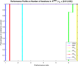
(a)

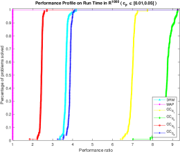
(b)

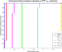
(c)

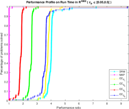
(d)

Figure 1: Performance profiles on six solvers for $c_{F}\in[0.01,0.5[$

From Figure 2(a)(b), we know that when $c_{F}\in[0.5,0.9[$, the number of iterations required by $CC_{\mathcal{S}_{2}}$ and $CC_{\mathcal{S}_{3}}$ are similar (the lines from $CC_{\mathcal{S}_{2}}$ and $CC_{\mathcal{S}_{3}}$ almost overlap) and dominate the other 4 algorithms, and $CC_{\mathcal{S}_{2}}$ is the fastest followed closely by MAP and $CC_{\mathcal{S}_{3}}$. By Figure 2(c)(d), we find that when $c_{F}\in[0.9,0.95[$ in which case MAP and DRM are very slow for solving the best approximation problem, $CC_{\mathcal{S}_{3}}$ needs the least number of iterations and is the fastest in every one of the 100 problems.

Note that in $\mathbb{R}^{1000}$, the calculation of projections takes the majority time in the whole time to solve the problems. As we mentioned before, we apply the Proposition 2.33 to calculate our circumcenter mappings: $CC_{\mathcal{S}_{1}}$, $CC_{\mathcal{S}_{2}}$, $CC_{\mathcal{S}_{3}}$ and $CC_{\mathcal{S}_{4}}$. Because the largest number of the operators in our $\mathcal{S}$ is $6$ (attained for $\mathcal{S}_{4}$), the size of the Gram matrix in Proposition 2.33 is less than or equal $5\times 5$. As it is shown in Figure 2(a)(c), the methods $CC_{\mathcal{S}_{2}}$, $CC_{\mathcal{S}_{3}}$ and $CC_{\mathcal{S}_{4}}$ need fewer iterations to solve the problems than MAP and DRM. It is well-known that MAP and DRM are very slow when $c_{F}$ is close to 1. It is not surprising that Figure 2(b) shows that $CC_{\mathcal{S}_{2}}$ is the fastest when for $c_{F}\in[0.5,0.9[$ and Figure 2(d) illustrates that $CC_{\mathcal{S}_{3}}$ is the fastest for $c_{F}\in[0.9,0.95[$.

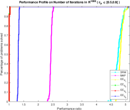
(a)

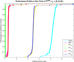
(b)

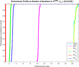
(c)

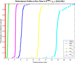
(d)

Figure 2: Performance profiles on six solvers for $c_{F}\in[0.5,0.95[$

The main conclusions that can be drawn from our experiments are the following.

When $c_{F}\in[0.01,0.5[$ is small, $CC_{\mathcal{S}_{4}}$ is the winner in terms of number of iterations and MAP is the best solver with consideration of the required run time. $CC_{\mathcal{S}_{3}}$ takes the second place in performance profiles with both of the performance measures 6.1 and 6.2 for $c_{F}\in[0.01,0.5[$.

When $c_{F}\in[0,5,0.9[$, Behling, Bello Cruz and Santos’ method $CC_{\mathcal{S}_{2}}$ is the optimal solver and the performance of $CC_{\mathcal{S}_{3}}$ is outstanding for both the required number of iterations and run time.

When $c_{F}\in[0,9,0.95[$, $CC_{\mathcal{S}_{3}}$ is the best option with regard to both required number of iterations and run time.

Altogether, if the user does not have an idea about the range of $c_{F}$, then we recommend $CC_{\mathcal{S}_{3}}$.

7 Concluding remarks

Generalizing some of our work in [5] and using the idea in [7], we showed the properness of the circumcenter mapping induced by isometries, which allowed us to study the circumcentered isometry methods. Sufficient conditions for the (weak, strong, linear) convergence of the circumcentered isometry methods were presented. In addition, we provided certain classes of linear convergent circumcentered reflection methods and established some of their applications. Numerical experiments suggested that three (including the C–DRM introduced in [7]) out of our four chosen circumcentered reflection methods dominated the DRM and MAP in terms of number of iterations for every pair of linear subspaces with the cosine of Friedrichs angle $c_{F}\in[0.01,0.95[$. Although MAP is fastest to solve the related problems when $c_{F}\in[0.01,0.5[$ and C–DRM is the fastest when $c_{F}\in[0.5,0.9[$, one of our new circumcentered reflection methods is a competitive choice when we have no prior knowledge on the Friedrichs angle $c_{F}$.

We showed the weak convergence of certain class of circumcentered isometry methods in Theorem 4.7. Naturally, we may ask whether strong convergence holds. If $\mathcal{S}$ consists of isometries and $\cap_{T\in\mathcal{S}}\operatorname{Fix}T\neq\varnothing$, then Theorem 3.3(i) shows the properness of $CC_{\mathcal{S}}$. Assuming additionally that $(CC_{\mathcal{S}}^{k}x)_{k\in\mathbb{N}}$ has a norm cluster in $\cap_{T\in\mathcal{S}}\operatorname{Fix}T$, Theorem 4.12(i) says that $(CC_{\mathcal{S}}^{k}x)_{k\in\mathbb{N}}$ converges to $\operatorname{P}_{\cap_{T\in\mathcal{S}}\operatorname{Fix}T}x$. Another question is: Can one find more general condition on $\mathcal{S}$ such that $CC_{\mathcal{S}}$ is proper and $(CC_{\mathcal{S}}^{k}x)_{k\in\mathbb{N}}$ has a norm cluster in $\cap_{T\in\mathcal{S}}\operatorname{Fix}T$ for some $x\in\mathcal{H}$? These are interesting questions to explore in future work.

Acknowledgements

The authors thank two anonymous referees and the editors for their constructive comments and professional handling of the manuscript. HHB and XW were partially supported by NSERC Discovery Grants.

References

- [1] H. H. Bauschke, J. Y. Bello Cruz, T. T. A. Nghia, H. M. Phan, and X. Wang, The rate of linear convergence of the Douglas-Rachford algorithm for subspaces is the cosine of the Friedrichs angle, Journal of Approximation Theory 185 (2014), pp. 63–79.
- [2] H. H. Bauschke and J. M. Borwein, On projection algorithms for solving convex feasibility problems, SIAM Review 38 (1996), pp. 367–426.
- [3] H. H. Bauschke and P. L. Combettes, Convex Analysis and Monotone Operator Theory in Hilbert Spaces, CMS Books in Mathematics, Springer, second ed., 2017.
- [4] H. H. Bauschke, H. Ouyang, and X. Wang, On circumcenters of finite sets in Hilbert spaces, Linear and Nonlinear Analysis 4 (2018), pp. 271–295.
- [5] H. H. Bauschke, H. Ouyang, and X. Wang, On circumcenter mappings induced by nonexpansive operators, Pure and Applied Functional Analysis, in press. arXiv preprint https://arxiv.org/abs/1811.11420, (2018).
- [6] H. H. Bauschke, H. Ouyang, and X. Wang, On the linear convergence of circumcentered isometry methods, arXiv preprint https://arxiv.org/abs/1912.01063, (2019).
- [7] R. Behling, J. Y. Bello Cruz, and L.-R. Santos, Circumcentering the Douglas–Rachford method, Numerical Algorithms 78 (2018), pp. 759–776.
- [8] R. Behling, J. Y. Bello Cruz, and L.-R. Santos, On the linear convergence of the circumcentered-reflection method, Operations Research Letters 46 (2018), pp. 159–162.
- [9] R. Behling, J. Y. Bello Cruz, and L.-R. Santos, The block-wise circumcentered-reflection method, arXiv preprint https://arxiv.org/abs/1902.10866, (2019).
- [10] N. Dizon, J. Hogan, and S. B. Lindstrom, Circumcentering reflection methods for nonconvex feasibility problems, arXiv preprint https://arxiv.org/abs/1910.04384, (2019).
- [11] F. Deutsch, Best Approximation in Inner Product Spaces, CMS Books in Mathematics, Springer-Verlag, New York, 2012.
- [12] E. D. Dolan and J. J. Moré, COPS. See http://www.mcs.anl.gov/~more/cops/.
- [13] E. D. Dolan and J. J. Moré, Benchmarking optimization software with performance profiles, Mathematical Programming 91 (2002), pp. 201–213.
- [14] W. B. Gearhart and M. Koshy, Acceleration schemes for the method of alternating projections, Journal of Computational and Applied Mathematics 26 (1989), pp. 235–249.
- [15] E. Kreyszig, Introductory Functional Analysis with Applications, John Wiley & Sons, Inc., New York, 1989.
- [16] S. B. Lindstrom, Computable centering methods for spiraling algorithms and their duals, with motivations from the theory of Lyapunov functions, arXiv preprint https://arxiv.org/abs/2001.10784, (2020).
- [17] C. Meyer, Matrix Analysis and Applied Linear Algebra, Society for Industrial and Applied Mathematics (SIAM), Philadelphia, PA, 2000.
- [18] R. T. Rockafellar, Convex Analysis, Princeton University Press, Princeton, NJ, 1997.