Signature of nonequilibrium quantum phase transition in the long time average of Loschmidt echo

Abstract

We unveil the role of the long time average of Loschmidt echo in the characterization of nonequilibrium quantum phase transitions by studying sudden quench processes across quantum phase transitions in various quantum systems. While the dynamical quantum phase transitions are characterized by the emergence of a series of zero points at critical times during time evolution, we demonstrate that nonequilibrium quantum phase transitions can be identified by nonanalyticities in the long time average of Loschmidt echo. The nonanalytic behaviours are illustrated by a sharp change in the long time average of Loschmidt echo or the corresponding rate function or the emergence of divergence in the second derivative of rate function when the driving quench parameter crosses the phase transition points. The connection between the second derivative of rate function and fidelity susceptibility is also discussed.

I INTRODUCTION

Over the past decades, quantum phase transitions (QPTs) have been attracted considerable attention in condense matter physics Sach . Contrary to the classical phase transitions driven by the temperature, QPTs occur at absolute zero temperature due to quantum fluctuations and are driven by physical parameters. According to Landau’s criteria, QPTs are characterized by singularities of the ground-state (GS) energy and a nth-order QPT is defined by discontinuities in the nth derivative of the energy. In recent years, some new approaches in quantum-information sciences shed light on the QPTs AO2002Nature ; TJO2002PRA ; GV2003PRL ; LA2008RMP and unveil the role of GS wavefunction in the characterization of QPTs QuanHT ; Zanardi ; GuSJ ; PZ2006PRE . One of the useful concepts is the GS fidelity, which is found to exhibit an abrupt drop at the phase transition point and can be applied to identify a QPT PZ2006PRE ; SC2007PRE ; ZHQ2008JPAMT41 ; SC2008PRA ; Zanardi ; GuSJ .

Meanwhile, QPTs far from equilibrium systems have extended our understanding of phase transitions and universality greatly TP2008PRL ; TP2011PRL ; Werner ; Altman ; MH2013PRL ; Sciolla ; Diehl ; Diehl-2008 ; Calabrese ; Polkovnikov . By a sudden change of the Hamiltonian, a quantum quench process can push the initial quantum system out of equilibrium, which permits us to study the quench dynamics of the nonequilibrium system. More recently, many researchers concentrated on critical phenomena presented in quench dynamics, which are termed dynamical quantum phase transitions (DQPTs) MH2013PRL ; CK2013PRB ; EC2014PRL ; FA2014PRB ; MM2014PRL ; JMH2014PRB ; MH2014PRL ; MH2015PRL ; MS2015PRB ; JCB2016PRB ; MH2018PRL ; YC17PRB ; Mera ; AA16LTP ; Heyl18RPP . An important quantity to describe DQPT is Loschmidt echo (LE), which measures the overlap of an initial quantum state and its time-evolved state after the quench Gorin . For the system with the initial state siting in ground state of a given Hamiltonian, it is found that the Loschmidt echo exhibits a series of zero points at critical times $\{t^{\ast}\}$ during time evolution if the post-quench Hamiltonian and initial Hamiltonian correspond to different phases. Corresponding to these zero points, the dynamical free energy density in the thermodynamic limit becomes nonanalytic as a function time, which is a characteristic feature of DQPT and has been verified in various systemsMH2013PRL ; CK2013PRB ; EC2014PRL ; FA2014PRB ; MM2014PRL ; JMH2014PRB ; MH2014PRL ; MH2015PRL ; MS2015PRB ; JCB2016PRB ; MH2018PRL ; YC17PRB . Review articles about DQPTs can be found in references AA16LTP ; Heyl18RPP . The LE has also been found applications in the context of decoherence QuanHT ; Rossini , quantum criticality Campbell ; Jafari ; WeiBB , out-of-equilibrium fluctuations Venuti ; Hamma and many-body localization MBL .

Besides the notation of DQPT, the concept of a steady-state transition was also proposed to describe the nonequilibrium QPT induced by quantum quench. In this notation, the nonequilibrium QPT is signaled by a nonanalytic change of physical properties as a function of the quench parameter in the asymptotic long-time state of the system Sciolla ; Diehl ; Diehl-2008 . Usually, time average of order parameter was used to characterize nonequilibrium criticality Silva2018 . The connection between the DQPT and steady-state transition was addressed recently Silva2018 ; Halimeh ; WangPei2018 . Although the notation of LE plays a particularly important role in the characterization of DQPT, its connection to the nonequilibrium QPT is not well understood yet.

In this work, we shall explore the role of long time average of LE in the characterization of nonequilibrium QPT. The long time average of LE is independent of time and conveys information of overlap of the initial state and eigenstats of the post-quench Hamiltonian. By studying several typical models which exhibit nonequilibrium QPTs, we demonstrate that the long time average of LE or closely related quantities display nonanalytic behavior when the quench parameter crosses a quantum phase transition point, suggesting that the nonanalytic change of long time average of LE can give signature of nonequilibrium QPT. For the specific case with the pre-quench and post-quench parameters being very close, we find that there exists an equivalent relation between the second derivative of rate function of long time average of LE and fidelity susceptibility, which indicates the existence of divergence in the second derivative of the rate function at the phase transition point.

II Long time average of Loschmidt echo and quench dynamics

II.1 long time average of Loschmidt echo

Without loss generality, we consider a general Hamiltonian undergoing a QPT described by $H(\lambda)$, where $\lambda$ is a control parameter which drives the QPT. Suppose the system is initially prepared as the ground state of the Hamiltonian $H(\lambda_{i})$, we investigate the quench dynamics by suddenly changing the driving parameter to $\lambda_{f}$, i.e., the sudden quench process is realized by a sudden change of the control parameter

$$\lambda(t)=\lambda_{i}\theta(-t)+\lambda_{f}\theta(t),$$

where $\lambda_{i}$ represents the control parameter in the initial (pre-quench) Hamiltonian, $\lambda_{f}$ the control parameter in the final (post-quench) Hamiltonian, and $\theta(t)$ is the Heaviside step function. Before studying concrete models, we shall briefly introduce the notation of LE and give the expression of long time average of LE. Given an initial quantum state $|\Psi(0)\rangle$, the Loschmidt amplitude is defined as

$$\mathcal{G}(t)=\langle\Psi(0)|\Psi(t)\rangle=\langle\Psi(0)|e^{-iH(\lambda_{f})t}|\Psi(0)\rangle,$$ (1)

which represents the overlap between the initial state and the time-evolved state after the quantum quench, and the Loschmidt echo is given by

$$\mathcal{L}(t)=|\mathcal{G}(t)|^{2}$$ (2)

which is the probability associated with Loschmidt amplitude. Traditionally, the ground state of the initial Hamiltonian is chosen as the initial state, and the Loschmidt echo could be interpreted as the return probability of the ground state during time evolution.

In this work, we mainly focus on the long time average of LE

$$\overline{\mathcal{L}}\equiv\lim_{\tau\rightarrow\infty}\frac{1}{\tau}\int_{0}^{\tau}|\mathcal{G}(t)|^{2}\mathtt{d}t.$$ (3)

By using

$$|\Psi(t)\rangle=e^{-iH(\lambda_{f})t}|\Psi(0)\rangle=\sum_{n}e^{-iE_{n}t}|\psi_{n}\rangle\langle\psi_{n}|\Psi(0)\rangle,$$

it follows

$$\overline{\mathcal{L}}(\lambda_{f})=\sum_{n}\left|\langle\psi_{n}(\lambda_{f})|\Psi(0)\rangle\right|^{4},$$ (4)

where the evolved state is expanded by the normalized eigenstates of $H(\lambda_{f})$ denoted by $|\psi_{n}\rangle$ with eigenenergy $E_{n}$. It can be found that the long time average of LE has a similar form of inverse participation ratio AD2013EPL , which gives the distribution information of the initial state in the Hilbert space of the post-quench Hamiltonian. In order to study critical properties of many-particle systems, we introduce the rate function of $\overline{\mathcal{L}}$ ,

$$\eta(\lambda_{f})=-\frac{1}{L}\log\overline{\mathcal{L}}(\lambda_{f}),$$ (5)

which is defined as the logarithm of $\overline{\mathcal{L}}$ divided by the system size $L$ and is an intensive quantity in the thermodynamic limit. When $\lambda_{f}$ approaches a critical point $\lambda_{c}$, $\eta(\lambda_{f})$ shall exhibit nonanalytic behaviours, which can be viewed as a characteristic signature of nonequilibrium quantum phase transition.

II.2 Quantum quench in the Aubry-André model

We first consider the Aubry-André (AA) model with Hamiltonian

$$H=-J\sum_{j=1}^{L-1}(c_{j}^{\dagger}c_{j+1}+h.c.)+\Delta\sum_{j=1}^{L}\cos(2\pi\alpha j)c_{j}^{\dagger}c_{j},$$ (6)

where $c_{j}^{\dagger}(c_{j})$ denotes the creation (annihilation) operator of fermions at site $j$ ($j=1,\cdots,L$ with $L$ the total number of lattice sites), $J$ is hopping amplitude and $\Delta$ is the strength of the incommensurate potential. Here $\alpha$ is an irrational number and we fix $\alpha=\frac{\sqrt{5}-1}{2}$ for convenience. The incommensurate potential strength $\Delta$ drives the system undergoing a delocalization-localization transition at a critical point $\Delta/J=2$. When $\Delta/J<2$, all the eigenstates are extended, but localized as $\Delta/J>2$. AA ; YC17PRB .

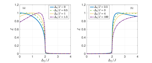
Figure 1: (Color online) The behavior of the long time average of LE of AA model with the total number of lattice sites $L=1000$. The strength of incommensurate potential in the initial Hamiltonian is (a) $\Delta_{i}/J=0,\,0.5,\,1,\,1.5$, (b) $\Delta_{i}/J=2.5,\,3,\,4,\,100$, respectively.

Now we consider the quench process described by the sudden change of the incommensurate potential strength $\Delta(t)=\Delta_{i}\theta(-t)+\Delta_{f}\theta(t)$, i.e., we prepare the initial state of system in the ground state of Hamiltonian $H(\Delta_{i})$, and then suddenly quench to Hamiltonian $H(\Delta_{f})$ at $t=0$. The DQPT in the AA model has been studied in Ref.YC17PRB . It was shown that the LE supports a series of zero points at critical times if $H(\Delta_{i})$ and $H(\Delta_{f})$ are in different phases. In Fig. 1, we display the long time average of LE versus $\Delta_{f}/J$ by fixing $\Delta_{i}/J=0,\,0.5,\,1,\,1.5$ (Fig.1(a)) and $\Delta_{i}/J=2.5,\,3,\,4,\,100$ (Fig.1(b)), respectively. For both cases, it is shown that $\overline{\mathcal{L}}$ has an obvious change around the transition point $\Delta_{f}/J=2$. Therefore, the sharp change of $\overline{\mathcal{L}}$ at the transition point can give us a characteristic signature of nonequilibrium quantum phase transition.

II.3 Quantum quench in the quantum Ising model

Next we consider the transverse field Ising model described by the following Hamiltonian

$$H=-J\sum_{j=1}^{L-1}\sigma_{j}^{x}\sigma_{j+1}^{x}+h\sum_{j=1}^{L}\sigma_{j}^{z}\,,$$ (7)

where $\sigma_{j}^{\alpha}$ , ($\alpha=x,y,z,$) are the Pauli matrices, $j=1,\cdots,L$ with $L$ the total number of lattice sites, $J$ is nearest-neighbor spin exchange interaction, and $h$ is the external magnetic field along the $z$ axis. The transverse field Ising model can be mapped to spinless fermions by using Jordan-Wigner transformation: $\sigma_{j}^{z}=2c_{j}^{\dagger}c_{j}-1$ and $\sigma_{j}^{x}=\prod_{i<j}(1-2c_{i}^{\dagger}c_{i})(c_{j}+c_{j}^{\dagger})$. In the fermion representation, we have

$$H=-J\sum_{j=1}^{L-1}\left(c_{j}^{\dagger}c_{j+1}+c_{j}^{\dagger}c_{j+1}^{\dagger}+h.c.\right)+2h\sum_{j=1}^{L}c_{j}^{\dagger}c_{j},$$ (8)

where we have discarded the constant $-hL$ which merely shifts the origin of energy and has no effect on the phase transition. Now, we consider the periodic boundary condition and use the Fourier transform $c_{j}^{{\dagger}}=\frac{1}{\sqrt{L}}\sum_{k}e^{ikj}c^{{\dagger}}(k)$, where $k$ is the wave vector and $-\pi<k\leqslant\pi$. In the momentum representation, the Bogoliubov–de Gennes Hamiltonian is given by

$$H_{k}=\left[\begin{array}[]{cc}-J\cos k+h&iJ\sin k\\ -iJ\sin k&J\cos k-h\end{array}\right].$$ (9)

Introducing a unitary transformation $\mathcal{H}_{k}=UH_{k}U^{-1}$ with

$$U=\frac{1}{\sqrt{2}}\left[\begin{array}[]{cc}1&-1\\ 1&1\end{array}\right],$$ (10)

then the Hamiltonian is transformed as

$$\mathcal{H}_{k}=\left[\begin{array}[]{cc}0&V(k)\\ V^{\ast}(k)&0\end{array}\right],$$ (11)

where $V(k)=h-Je^{-ik}$. The two eigenvalues are $E_{\pm}=\pm\sqrt{V(k)V^{\ast}(k)}$ and two eigenvectors are $|\psi_{\pm}\rangle=\frac{1}{\sqrt{2}}\left(\left(\frac{V(k)}{V^{\ast}(k)}\right)^{1/4},\pm\left(\frac{V^{\ast}(k)}{V(k)}\right)^{1/4}\right)^{\text{T}}$. There are two distinct phases which can be characterized by the winding number $\nu$ with the from

$$\nu=-\frac{1}{2\pi i}\int_{-\pi}^{\pi}V^{-1}(k)\partial_{k}V(k)dk\,,$$ (12)

where the winding number is either $0$ or $1$, depending on the parameters. It follows that the winding number $\nu=1$ for $|h/J|\leqslant 1$ corresponding to the topological phase, otherwise $\nu=0$ represents the trivial phase. We focus on the region of $h/J\geqslant 0$ and the phase transition point is given by $h_{c}/J=1$.

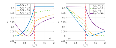
Figure 2: (Color online) The behavior of $\eta$ of Ising model with respect to external magnetic field $h_{f}$ of the post-quench Hamiltonian. The total number of lattice sites $L=1000$. The red dashed vertical line in figures guides the value of the phase transition point $h_{c}/J=1$. The external magnetic field along the $x$ axis in the intital Hamiltonian is (a) $h_{i}/J=0,\,0.2,\,0.5,\,0.7$, (b) $h_{i}/J=1.2,\,1.5,\,2,\,100$, respectively.

Now we consider the quench process with $h(t)=h_{i}\theta(-t)+h_{f}\theta(t)$. We prepare the ground state of quantum Ising model $H(h_{i})$ in fermion representation as the initial state. For convenience, we can calculate the rate function of the long time average of LE which has the form

$$\eta(h_{f}) = -\frac{1}{L}\log\left[\sum_{\alpha_{1}\cdots\alpha_{N}=\pm}\left|\vphantom{\sum_{a}}\left(\langle\phi_{\alpha_{1}}(k_{1})|\otimes\cdots\otimes\langle\phi_{\alpha_{N}}(k_{N})|\right)\right.\right.$$ (13)

$$\left.\left.\times\left(|\psi_{-}(k_{1})\rangle\otimes\cdots\otimes|\psi_{-}(k_{N})\rangle\right)\vphantom{\sum_{a}}\right|^{4}\mathstrut\vphantom{\sum_{\alpha_{1}}}\right].$$

In the limit of $L\rightarrow\infty$, the momentum $k$ distributes continuously and we can get

$$\eta(h_{f})=-\frac{1}{2\pi}\int_{-\pi}^{\pi}\text{d}k\left[\log\sum_{\alpha=\pm}\left|\vphantom{\sum}\langle\phi_{\alpha}(k)|\psi_{-}(k)\rangle\right|^{4}\right],$$ (14)

where $|\psi_{-}(k)\rangle$ is the ground state wavefunction of the initial Hamiltonian $\mathcal{H}_{k}(h_{i})$. Then the time evolution is governed by the final Hamiltonian $\mathcal{H}_{k}(h_{f})$ with two eigenvalues $E_{\pm}(h_{f})$ and two corresponding wavefunctions are $|\phi_{\alpha}(k)\rangle$ ($\alpha=\pm$). Substituting the concrete form of $V(k)$ in $|\psi_{-}(k)\rangle$ and $|\phi_{\alpha}(k)\rangle$. Then $\eta$ can be written as

$$\eta=-\frac{1}{2\pi}\int_{-\pi}^{\pi}\text{d}k\left[\log\frac{1+\cos^{2}\theta}{2}\right]$$ (15)

with

$$\theta=\arctan\frac{\left(h_{f}/J-h_{i}/J\right)\sin k}{1+h_{i}h_{f}/J^{2}-\left(h_{i}/J+h_{f}/J\right)\cos k},$$

where $h_{i}/J$ and $h_{f}/J$ are external magnetic field along the $x$ axis in the initial and final Hamiltonian, respectively.

We numerically calculate Eq.(15) and show several results with different initial Hamiltonian in Fig.2. For Fig.2(a), taking the initial state prepared in the phase with $h_{i}/J=0$ and $\nu=1$ (solid line) as an example, we can see that $\eta$ grows from $0$ to the value approximately equal to $0.315$ as $h_{f}/J$ increases from $0$ to the critical point $h_{c}/J=1$, where $\eta=0$ means the final state is the same as the initial state with $h_{i}=h_{f}$. When the parameter $h_{f}/J$ crosses the critical point, the final Hamiltonian enters into the trivial phase with $\nu=0$, and $\eta$ keeps approximately to be a constant with the increasing of $h_{f}/J$. In Fig.2(b), taking the initial Hamiltonian in the trivial phase with $h_{i}/J=100$ and $\nu=0$ (solid line) as an example, and continuously change the parameter $h_{f}/J$ of final Hamiltonian from $0$ to $2$. It can be seen that $\eta$ remains a constant approximately equal to $0.315$ when the final Hamiltonian is in the topological phase with $h_{f}\leqslant h_{c}$. After crossing the critical point $h_{c}/J$ with $h_{f}>h_{c}$, $\eta$ begins to decrease with the increase of $h_{f}$ and shall reach the minimum value $0$ at $h_{i}=h_{f}$. Generally, we can see the nonanalyticity of $\eta$ emerges as long as $h_{f}$ crosses the critical point and is independent of the choice of the initial state. Nonequilibrium QPT is characterized by the nonanalytic behavior of $\eta$ at the critical point.

II.4 Quantum quench in the Haldane model

In this subsection, we investigate the Haldane model Haldane described by the following tight-binding Hamiltonian

$${H=M\sum_{j}\left[c_{A,\vec{r}_{j}}^{{\dagger}}c_{A,\vec{r}_{j}}-c_{B,\vec{r}_{j}}^{{\dagger}}c_{B,\vec{r}_{j}}\right]+H_{\text{NN}}+H_{\text{NNN}}},$$ (16)

with

$$H_{\text{NN}} = -t_{1}\sum_{j}\left[c_{A,\vec{r}_{j}}^{{\dagger}}c_{B,\vec{r}_{j}+\widehat{e}_{1}}+c_{A,\vec{r}_{j}}^{{\dagger}}c_{B,\vec{r}_{j}+\widehat{e}_{2}}\right.$$ (17)

$$+\left.c_{A,\vec{r}_{j}}^{{\dagger}}c_{B,\vec{r}_{j}+\widehat{e}_{3}}+h.c.\right],$$

and

$$H_{\text{NNN}} = -t_{2}e^{i\phi}\sum_{j}\left[c_{A,\vec{r}_{j}}^{{\dagger}}c_{A,\vec{r}_{j}+\widehat{\nu}_{1}}+c_{A,\vec{r}_{j}}^{{\dagger}}c_{A,\vec{r}_{j}+\widehat{\nu}_{2}}\right.$$ (18)

$$+\left.c_{A,\vec{r}_{j}}^{{\dagger}}c_{A,\vec{r}_{j}+\widehat{\nu}_{3}}+(A\rightarrow B)+h.c.\right],$$

where the on-site energy is $M$ on $A$ sites and $-M$ on $B$ sites, $H_{\text{NN}}$ denotes the Hamiltonian with nearest-neighbor (NN) hopping amplitude $t_{1}$, and $H_{\text{NNN}}$ the Hamiltonian with next-nearest-neighbor (NNN) hopping amplitude $t_{2}$ and phase difference $\phi$, Here $c_{\alpha,\vec{r}_{j}}^{\dagger}(c_{\vec{r}_{j}})$ denotes the creation (annihilation) operator of fermions at the sublattice $\alpha=A,B$ of site $\vec{r}_{j}$. The summation is defined on a two-dimensional honeycomb lattice. The illustration of honeycomb lattice of Haldane model is shown in Fig.3(a), where $\hat{e}_{1}=(0,a)$, $\hat{e}_{2}=(-\frac{\sqrt{3}}{2}a,-\frac{1}{2}a)$ and $\hat{e}_{3}=(\frac{\sqrt{3}}{2}a,-\frac{1}{2}a)$ are the displacements from a $A$ site located at $\vec{r}_{j}$ to its three nearest-neighbor $B$ sites, and $\hat{\nu}_{1}=(\sqrt{3}a,0)$, $\hat{\nu}_{2}=(-\frac{\sqrt{3}}{2}a,\frac{3}{2}a)$ and $\hat{\nu}_{3}=(-\frac{\sqrt{3}}{2}a,-\frac{3}{2}a)$ are the displacements from a $A$ site located at $\vec{r}_{j}$ to its three distinct next-nearest-neighbor $A$ sites. Here $a$ is lattice constant and we shall fix $a=1$.

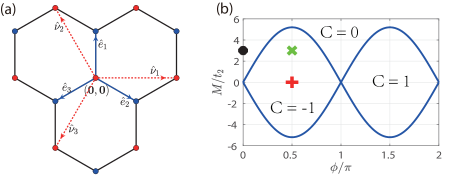
Figure 3: (Color online) (a) Illustration of the honeycomb lattice. Red and blue circles represent two sublattices (A and B). Three blue lines with arrow denote three nearest-neighbor displacements of A, and three red dashed lines with arrow denote three distinct next-nearest-neighbor displacements of A. (b) Phase diagram of Haldane model. Red plus sign marks the initial state for Fig.4. Black dot marks the initial state for Fig.5(a) and (b) and green times sign marks the initial state for Fig.5(c) and (d).

By taking the periodic boundary condition along the $x$-axis and $y$-axis direction, the Hamiltonian in momentum space can be written as

$$H_{k}=\left[\begin{array}[]{cc}M-2t_{2}\sum_{j=1}^{3}\left[\cos\phi\cos(\mathbf{k\cdot}\widehat{\nu}_{j})-\sin\phi\sin(\mathbf{k\cdot}\widehat{\nu}_{j})\right]&-t_{1}\sum_{j=1}^{3}\left[\cos(\mathbf{k\cdot}\widehat{e}_{j})-i\sin(\mathbf{k\cdot}\widehat{e}_{j})\right]\\ -t_{1}\sum_{j=1}^{3}\left[\cos(\mathbf{k\cdot}\widehat{e}_{j})+i\sin(\mathbf{k\cdot}\widehat{e}_{j})\right]&-M-2t_{2}\sum_{j=1}^{3}\left[\cos\phi\cos(\mathbf{k\cdot}\widehat{\nu}_{j})-\sin\phi\sin(\mathbf{k\cdot}\widehat{\nu}_{j})\right]\end{array}\right],$$ (19)

where $\mathbf{k}$ is the wavevector in the first Brillouin zone (FBZ). The topologically different phases of Haldane model can be characterized by Chern number with the form Haldane

$$C=\frac{1}{2\pi}\int_{\text{FBZ}}\Omega_{n}(\mathbf{k)}\text{d}\mathbf{k}\,,$$ (20)

where $\Omega_{n}(\mathbf{k)}$ is the Berry curvature of the $n$-th band with the Berry connection $\mathcal{A}_{n}(\mathbf{k})=-i\langle\phi_{n}(\mathbf{k)}|\nabla_{\mathbf{k}}|\phi_{n}(\mathbf{k)}\rangle$. The phase diagram in the $(\phi,M)$ plane is shown in Fig.3(b). While the regime of $C=0$ represents the topologically trivial phase, regimes with $C=\pm 1$ represent topological phases.

Now we consider the quench process solely driven by either the parameter $M$ or the phase difference $\phi$, i.e., the sudden quench described by $M(t)=M_{i}\theta(-t)+M_{f}\theta(t)$ or $\phi(t)=\phi_{i}\theta(-t)+\phi_{f}\theta(t)$. Similarly, we calculate the rate function of the long time average of LE, which takes the following form:

$$\eta=-\frac{1}{L}\sum_{j}\left[\log\sum_{\alpha_{j}=\pm}\left|\vphantom{\sum}\langle\phi_{\alpha_{j}}(\mathbf{k}_{j})|\psi_{-}(\mathbf{k}_{j})\rangle\right|^{4}\right],$$ (21)

where $L$ is the total number of lattice sites. As the system approaches the thermodynamic limit, the rate function of the long time average of LE takes the continuous form:

$$\eta=-\frac{1}{S_{k}}\int_{\text{FBZ}}\text{d}\mathbf{k}\left[\log\sum_{\alpha=\pm}\left|\vphantom{\sum}\langle\phi_{\alpha}(\mathbf{k})|\psi_{-}(\mathbf{k})\rangle\right|^{4}\right],$$ (22)

where $S_{k}$ is the area of FBZ, $|\psi_{-}(\mathbf{k})\rangle$ is the ground state wavefunction of the initial Hamiltonian in momentum space, and $|\phi_{\pm}(\mathbf{k})\rangle$ are wavefunctions of the final Hamiltonian. By preparing the initial state in the topologically nontrivial phase with $M_{i}=0$, $\phi=0.5\pi$ and $C=-1$ corresponding to the red plus sign marked in Fig.3(b), we study the quench dynamics driven by the final Hamiltonian with different $M_{f}$. The behaviour of $\eta$ versus $M_{f}$ is illustrated in Fig.4(a). As $\eta$ grows from $0$ with increasing $M_{f}$ from $0$ to $8$, no an obvious change is observed when $M_{f}$ crosses the phase transition point. Nevertheless, we can define the quantity $\chi_{\lambda_{f}}$ which is equal to the minus of the second derivative of $\eta$ with respect to the post-quench parameter $\lambda_{f}$:

$$\chi_{\lambda_{f}}=-\frac{\partial^{2}\eta}{\partial\lambda_{f}^{2}}\,.$$ (23)

We find that $\chi_{M_{f}}$ exhibits discontinuity with an obvious peak around $M_{f}=3\sqrt{3}$ as shown in Fig.4(b). The value of $M_{f}$ at discontinuous point of $\chi_{M_{f}}$ is exactly equal to the value of topological phase transition point calculated by Chern number.

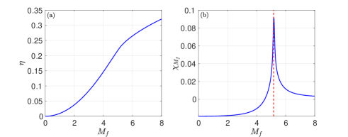
Figure 4: (Color online) (a) The behavior of $\eta$ of Haldane model with respect to on-site energy $M_{f}$ of the final Hamiltonian. (b) The second derivative of $\eta$ versus $M_{f}$. The red dashed line in figure guides the value of the topological phase transition point. We have taken $t_{1}=4,t_{2}=1,$ and $\phi=\pi/2$. The total number of lattice sites is $L=30082$. The on-site energy of the initial Hamiltonian is $M_{i}=0$.

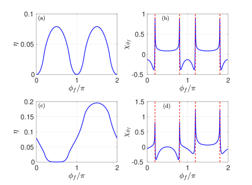
Figure 5: (Color online) (a) The behavior of $\eta$ of Haldane model with respect to $\phi_{f}$ of the final Hamiltonian. (b) The second derivative of $\eta$ versus $\phi_{f}$. The red dashed lines in the figure guide the values of the topological phase transition points which are calculated by Chern number. We have taken $t_{1}=4$, $t_{2}=1$ and $M=3$. The total number of lattice sites is $L=30082$. The phase difference of initial Hamiltonian is (a), (b) $\phi_{i}=0$, and (c), (d) $\phi_{i}=\pi/2$.

Next, we study the quench dynamics driven by the final Hamiltonian with different $\phi_{f}$. The initial state corresponding to Fig.5(a),(b) is prepared in the topologically trivial phase with $M_{i}=3\sqrt{3},\phi=0$ and $C=0$ as marked by black dot in Fig.3(b), and the initial state corresponding to Fig.5(c),(d) is prepared in the topologically nontrivial phase with $M_{i}=3\sqrt{3},\phi=0.5\pi$ and $C=-1$ as marked by green times sign in Fig.3(b). We display $\eta$ versus $\phi_{f}$ in Fig.5(a) and $\chi_{\phi_{f}}$ versus $\phi_{f}$ in Fig.5(b). While no obvious nonanalyticity is found in Fig.5(a), $\chi_{\phi_{f}}$ exhibits discontinuities with obvious peaks at $\phi_{f}\approx 0.194\pi,0.802\pi,1.194\pi$ and $1.802\pi$, corresponding to the phase boundaries in the phase diagram of Fig.3(b). For the initial state prepared in the topological phase with $\phi_{i}=\pi/2$, we display $\eta$ versus $\phi_{f}$ in Fig.5(c) and $\chi_{\phi_{f}}$ versus $\phi_{f}$ in Fig.5(d). Similarly, we identify four divergent points at $\phi_{f}\approx 0.194\pi,0.802\pi,1.194\pi$ and $1.802\pi$ in Fig.5(d), whose positions are identical to those displayed in Fig.5(b).

Our results indicate that $\chi_{\lambda_{f}}$ exhibits singular behavior with the emergence of an obvious peak when the driving parameter crosses the phase transition point, regardless of our choice of initial state. In Fig.6, we display $\chi_{\lambda_{f}}$ for different lattice sizes. Despite no real divergence for the finite size system, it is shown that the height of peak increasing with the lattice size, suggesting the existence of divergence in the thermodynamic limit.

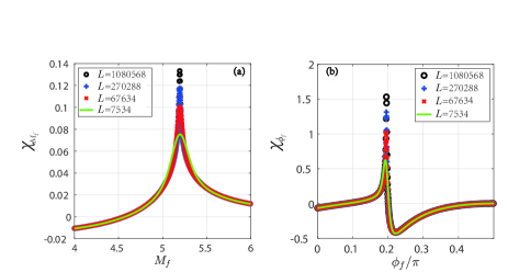
Figure 6: (Color online) $\chi_{\lambda_{f}}$ versus $\lambda_{f}$ for different lattice sizes. The parameters are $t_{1}=4$ and $t_{2}=1$. (a) $\phi=\pi/2$ and on-site energy of the initial Hamiltonian $M_{i}=0$. (b) $M=3$ and phase difference of the initial Hamiltonian $\phi_{i}=\pi/2$ .

II.5 Relation to fidelity susceptibility

We consider the limiting case that the driving parameters before and after sudden quench are very close, i.e., $\lambda_{i}=\lambda$ and $\lambda_{f}=\lambda+\delta$ with $\delta$ being a small quantity. Without loss generality, we suppose that $H(\lambda)=H_{0}+\lambda H_{1}$. Since the initial state is taken as the ground state of $H(\lambda)$, i.e., $\Psi(0)=\psi_{0}(\lambda)$, we have

$$\overline{\mathcal{L}}_{\delta}=\sum_{n}\left|\langle\psi_{n}(\mathbf{\lambda+\delta})|\psi_{0}(\mathbf{\lambda})\rangle\right|^{4}.$$ (24)

Expanding the wave function $|\psi_{0}(\mathbf{\lambda}+\delta)\rangle$ in the basis of eigenstates corresponding to the parameter $\lambda$, to the first order of $\delta$, we get

$$|\psi_{n}(\lambda+\delta)\rangle=c_{n}\left(|\psi_{n}(\mathbf{\lambda})\rangle+\delta\sum_{m\neq n}\frac{H_{mn}|\psi_{m}(\mathbf{\lambda})\rangle}{E_{n}(\lambda)-E_{m}(\lambda)}\right),$$ (25)

where $c_{n}=\left\{1+\delta^{2}\sum_{m\neq n}|H_{mn}|^{2}/\left[E_{n}(\lambda)-E_{m}(\lambda)\right]^{2}\right\}^{-1/2}$ are the normalization constants and $H_{mn}=\langle\psi_{m}(\mathbf{\lambda})|H_{1}|\psi_{n}(\mathbf{\lambda})\rangle$. Substituting the conjugation of Eq.(25) into Eq.(24) and expanding $\overline{\mathcal{L}}_{\delta}$ to the second order of $\delta$, we have

$$\overline{\mathcal{L}}_{\delta}=1-2\delta^{2}\sum_{m\neq 0}\frac{\left|H_{m0}\right|^{2}}{\left[E_{0}(\lambda)-E_{m}(\lambda)\right]^{2}}.$$ (26)

Then, the term which defines the response of the $\overline{\mathcal{L}}_{\delta}$ to a small change in $\delta$ can be obtained as

$$\chi_{\delta}=-\frac{\partial^{2}\overline{\mathcal{L}}_{\delta}}{\partial\delta^{2}}=\sum_{m\neq 0}\frac{4\left|H_{m0}\right|^{2}}{\left[E_{0}(\lambda)-E_{m}(\lambda)\right]^{2}}\,.$$ (27)

Now we explore the relation between $\chi_{\delta}$ and the fidelity susceptibility. We notice that the ground state fidelity is defined as the overlap of wavefunctions with driving parameter $\lambda$ and $\lambda+\delta$ PZ2006PRE , i.e.,

$$\mathcal{F}=\left|\langle\psi_{0}(\mathbf{\lambda}+\delta)|\psi_{0}(\mathbf{\lambda})\rangle\right|\,.$$ (28)

Substituting the conjugation of Eq.(25) into Eq.(28), we have

$$\mathcal{F}=\left(1+\delta^{2}\sum_{m\neq 0}\frac{\left|H_{m0}\right|^{2}}{\left[E_{0}(\lambda)-E_{m}(\lambda)\right]^{2}}\right)^{-1/2},$$ (29)

and the fidelity susceptibility is given by GuSJ ; Zanardi

$$\mathcal{\chi}_{\mathcal{F}}=-\frac{\partial^{2}\mathcal{F}}{\partial\delta^{2}}=\sum_{m\neq 0}\frac{\left|H_{m0}\right|^{2}}{\left[E_{0}(\lambda)-E_{m}(\lambda)\right]^{2}}\,.$$ (30)

The connection of fidelity susceptibility and the Berry curvature was discussed in the reference Zanardi . A review article for the role of fidelity and fidelity susceptibility in the characterization of static QPTs can be found in the reference GuSJ2 . In comparison with Eq.(27), it is straightforward to find the following relation:

$$\chi_{\delta}=4\mathcal{\chi}_{\mathcal{F}}\,.$$ (31)

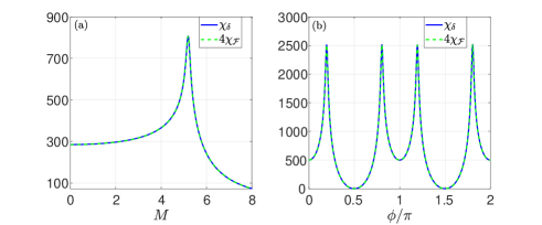
Figure 7: (Color online) (a) $\chi_{\delta}$ and $4\mathcal{\chi}_{\mathcal{F}}$ versus $M$. For the quench process, we take $M_{i}=M$ and $M_{f}=M+\delta$. The parameters are $\delta=10^{-5}$ and $\phi=\pi/2$. (b) $\chi_{\delta}$ and $4\mathcal{\ \chi}_{\mathcal{F}}$ versus $\phi$. Here we take $\phi_{i}=\phi$ and $\phi_{f}=\phi+\delta$. The parameters are $\delta=10^{-5}$ and $M=3$.

In Fig.7 (a) and (b) we numerically illustrate $\chi_{\delta}$ and $4\mathcal{\chi}_{\mathcal{F}}$ versus $M$ and $\phi$ for the Haldane model, respectively. It is found that the two curves are identical, consistent with the analytical relation given by Eq.(31). It is well known that the fidelity susceptibility is divergent at the phase transition point GuSJ ; SC2008PRA ; Zanardi . The relation between $\chi_{\delta}$ and $\mathcal{\chi}_{\mathcal{F}}$ suggests the existence of divergence in $\chi_{\delta}$ around the phase transition point.

III Summary

In summary, we have studied the long time average of LE for the sudden quench processes in various quantum systems, including the AA model, quantum Ising model and Haldane model, and shown that the long time average of LE $\overline{\mathcal{L}}(\lambda_{f})$ or its rate function $\eta(\lambda_{f})$ exhibits nonanalytic behavior when the quench parameter crosses the phase transition points. For the AA model and quantum Ising model, we demonstrated that as quench parameter varies across a phase transition point, the long time average of LE or its rate function has an obviously sudden change around the transition point. For the Haldane model, the nonanalyticity of the rate function at the phase transition point is not so obvious. But we found the quantity $\chi_{\lambda_{f}}$ which is proportional to the second derivative of rate function exhibits a divergent peak as the quench parameter crosses the phase transition points. Considering the limiting case that the pre-quench and post-quench parameters are very close, we analytically proved that $\chi_{\delta}$ is proportional to the fidelity susceptibility as $\delta\rightarrow 0$. The connection with fidelity susceptibility suggest that the long time average of LE and its rate function can be used to signal nonequilibrium QPTs in more general systems.

- (1) S. Sachdev, Quantum Phase Transitions (Cambridge University Press, Cambridge, England, 1999).
- (2) A. Osterloh, L. Amico, G. Falci, and Rosario Fazio, Nature(London) 416, 608 (2002).
- (3) T. J. Osborne and M. A. Nielsen, Phys. Rev. A 66, 032110 (2002).
- (4) G. Vidal, J. I. Latorre, E. Rico, and A. Kitaev, Phys. Rev. Lett.90, 227902 (2003).
- (5) L. Amico, R. Fazio, A. Osterloh, and V. Vedral Rev. Mod. Phys. 80, 517 (2008).
- (6) H. T. Quan, Z. Song, X. F. Liu, P. Zanardi, and C. P. Sun, Phys. Rev. Lett. 96, 140604 (2006).
- (7) P. Zanardi and N. Paunković, Phys. Rev. E 74, 031123 (2006).
- (8) W. L. You, Y. W. Li, and S. J. Gu, Phys. Rev. E 76, 022101 (2007).
- (9) L. Campos Venuti and P. Zanardi, Phys. Rev. Lett. 99, 095701 (2007); P. Zanardi, P. Giorda, and M. Cozzini, ibid. 99, 100603 (2007).
- (10) S. Chen, L. Wang, Y. Hao, and Y. Wang, Phys. Rev. A 77, 032111 (2008).
- (11) S. Chen, L. Wang, S. J. Gu, and Y. Wang, Phys. Rev. E 76, 061108 (2007).
- (12) H. Q. Zhou and J. P. Barjaktarevič, J. Phys. A: Math. Theor. 41, 412001 (2008).
- (13) T. Prosen and I. Pižorn, Phys. Rev. Lett, 101, 105701 (2008).
- (14) S. Diehl, A. Micheli, A. Kantian, B. Kraus, H. P. Buechler, and P. Zoller, Nat. Phys. 4, 878 (2008).
- (15) S. Diehl, A. Tomadin, A. Micheli, R. Fazio, and P. Zoller, Phys. Rev. Lett. 105, 015702 (2010).
- (16) B. Sciolla and G. Biroli, Phys. Rev. Lett. 105, 220401 (2010).
- (17) P. Barmettler, M. Punk, V. Gritsev, E. Demler, and E. Altman, Phys. Rev. Lett. 102, 130603 (2009).
- (18) M. Eckstein, M. Kollar, and P. Werner, Phys. Rev. Lett. 103, 056403 (2009).
- (19) T. Prosen and E. Ilievski, Phys. Rev. Lett, 107, 060403 (2011).
- (20) P. Calabrese, F. H. L. Essler, and M. Fagotti, J. Stat. Mech. (2012) P07016; ibid, (2012) P07022.
- (21) A. Polkovnikov, K. Sengupta, A. Silva, and M. Vengalatorre, Rev. Mod. Phys. 83, 863 (2011).
- (22) M. Heyl, A. Polkovnikov, and S. Kehrein, Phys. Rev. Lett, 110, 135704 (2013)
- (23) C. Karrasch and D. Schuricht, Phys. Rev. B 87, 195104 (2013).
- (24) E. Canovi, P. Werner, and M. Eckstein, Phys. Rev. Lett. 113, 265702 (2014).
- (25) F. Andraschko and J. Sirker, Phys. Rev. B 89, 125120 (2014).
- (26) M. Marcuzzi, E. Levi, S. Diehl, J. P. Garrahan, and I. Lesanovsky, Phys. Rev. Lett. 113, 210401 (2014).
- (27) J. M. Hickey, S. Genway, and J. P. Garrahan, Phys. Rev. B 89, 054301 (2014).
- (28) M. Heyl, Phys. Rev. Lett. 113, 205701 (2014).
- (29) M. Heyl, Phys. Rev. Lett. 115, 140602 (2015).
- (30) M. Schmitt and S. Kehrein, Phys. Rev. B 92, 075114 (2015).
- (31) J. C. Budich and M. Heyl, Phys. Rev. B 93, 085416 (2016).
- (32) M. Heyl, F. Pollmann, and B. Dóra, Phys. Rev. Lett. 121, 016801 (2018).
- (33) C. Yang, Y. Wang, P. Wang, X. Gao and S. Chen, Phys. Rev. B 95, 184201 (2017).
- (34) B. Mera, C. Vlachou, N. Paunković, V. R. Vieira, and O. Viyuela, Phys. Rev. B 97, 094110 (2018).
- (35) A. A. Zvyagin, Fiz. Nizk. Temp. 42, 1240 (2016) [Low Temp. Phys. 42, 971 (2016)].
- (36) M. Heyl, Rep. Progr. Phys. 81, 054001 (2018).
- (37) T. Gorin, T. Prosen, T. H. Seligman, and M. Znidaric, Phys. Rep. 435, 33 (2006).
- (38) D. Rossini, T. Calarco, V. Giovannetti, S. Montangero, and R. Fazio, Phys. Rev. A 75, 032333 (2007).
- (39) S. Campbell, Phys. Rev. B 94, 184403 (2016).
- (40) R. Jafari and H. Johannesson, Phys. Rev. Lett. 118, 015701 (2017).
- (41) M.-J. Hwang, B.-B. Wei, S. F. Huelga, and M. B. Plenio, arXiv:1904.09937.
- (42) L. Campos Venuti and P. Zanardi, Phys. Rev. A 81, 022113 (2010).
- (43) J. Yang and A. Hamma, arXiv:1702.00445.
- (44) M. Serbyn and D. A. Abanin, Phys. Rev. B 96, 014202 (2017).
- (45) B. Zunkovic, M. Heyl, M. Knap, and A. Silva, Phys. Rev. Lett. 120, 130601 (2018).
- (46) P. Wang and Gao Xianlong Phys. Rev. A 97, 023627 (2018).
- (47) J. C. Halimeh and V. Zauner-Stauber, Phys. Rev. B 96, 134427 (2017).
- (48) A. Deluca and A. Scardicchio, Europhys. Lett 101 37003 (2013).
- (49) S. Aubry and G. André, Ann. Isr. Phys. Soc. 3, 133 (1980).
- (50) F. D. M. Haldane, Phys. Rev. Lett. 61, 2015 (1988).
- (51) S. J. Gu, Int. J. Mod. Phys. B 24, 4371 (2010).