• We derive an explicit expression for the leading term in the late-time, large-distance asymptotic expansion of a transverse dynamical two-point function of the XX chain in the spacelike regime. This expression is valid for all non-zero finite temperatures and for all magnetic fields below the saturation threshold. It is obtained here by means of a straightforward term-by-term analysis of a thermal form factor series, derived in previous work, and demonstrates the usefulness of the latter.

1 Introduction

The XX chain is a spin chain with Hamiltonian [15]

$$H_{L}=J\sum_{j=1}^{L}\bigl{(}\sigma_{j-1}^{x}\sigma_{j}^{x}+\sigma_{j-1}^{y}\sigma_{j}^{y}\bigr{)}-\frac{h}{2}\sum_{j=1}^{L}\sigma_{j}^{z}\,,$$ (1)

where the $\sigma_{j}^{\alpha}$, $\alpha=x,y,z$, are Pauli matrices acting on site $j\in\{1,\dots,L\}$ of an $L$-site periodic lattice, $\sigma_{0}^{\alpha}=\sigma_{L}^{\alpha}$. The parameters $J>0$ and $h>0$ denote the strengths of the spin-spin interaction and of the applied magnetic field. We shall restrict the magnetic field to values below the saturation threshold, $0<h<4J$.

In our recent work [9] we have derived a novel form factor series for the transverse dynamical correlation function

$$\bigl{\langle}\sigma_{1}^{-}\sigma_{m+1}^{+}(t)\bigr{\rangle}_{T}=\lim_{L\rightarrow+\infty}\frac{\operatorname{tr}\{{\rm e}^{-H_{L}/T}\sigma_{1}^{-}{\rm e}^{{\rm i}H_{L}t}\sigma_{m+1}^{+}{\rm e}^{-{\rm i}H_{L}t}\}}{\operatorname{tr}\{{\rm e}^{-H_{L}/T}\}}$$ (2)

of the XX chain in equilibrium with a heat bath at temperature $T$. It measures the space-time evolution of a local perturbation relating two points at distance $m$ and temporal separation $t$. Our series originates from a form factor expansion related to the quantum transfer matrix [7]. It can be resummed into a ‘Fredholm determinant representation’ consisting of a prefactor times a Fredholm determinant of an integrable integral operator [11]. The latter is different from the Fredholm determinant representation derived by Colomo et al. in [5].

For Fredholm determinants and resolvent kernels of integrable integral operators a general method [6] is available that allows one to analyse their asymptotic dependence on parameters. Starting with the Fredholm determinant representation obtained in [5] the authors of [12] applied this ‘nonlinear steepest-descent method’ to the late-time, large-distance analysis of (2) at a fixed ratio $\alpha=m/(4Jt)$. They found exponential decay of the form

$$\bigl{\langle}\sigma_{1}^{-}\sigma_{m+1}^{+}(t)\bigr{\rangle}_{T}\sim Ct^{\nu}{\rm e}^{-m/\xi}\,,$$ (3)

where $C$, $\nu$ and $\xi$ depend on $T$, $h$ and $\alpha$. The functional dependence differs according to whether $\alpha>1$ or $\alpha<1$. The former regime, in which the spatial distance in units of $4J$ is larger than the temporal separation, is called ‘spacelike’, while the latter is referred to as ‘the timelike regime’.

In [12] the authors considered magnetic fields below the saturation threshold, $0<h<4J$. They obtained explicit expressions for $\nu$ and $\xi$ in both, space- and timelike regimes. Later the ‘constant term’ $C$ was obtained for $h>4J$ in [13]. Although the nonlinear steepest descent method would allow one to calculate $C$ for $0<h<4J$ as well, it seems that nobody has ever attempted to do so. This may be partially attributed to the cumbersome nature of the required calculations.

In this work we reconsider the late-time, large-distance asymptotic analysis of the two-point function $\langle\sigma_{1}^{-}\sigma_{m+1}^{+}(t)\bigr{\rangle}_{T}$ in the spacelike regime. It turns out that the novel thermal form factor series derived in [9] allows us to obtain the asymptotics, including the constant term $C$, by a rather elementary term-by-term analysis of the series that avoids the use of any Riemann-Hilbert problem.

On the other hand, our thermal form factor series can be resummed into a Fredholm determinant representation as well. As we shall see below this Fredholm determinant representation is rather different from the one of Its et al. [12] in that the term that provides the leading late-time, large-distance asymptotics in the spacelike regime appears to be pulled out as a pre-factor. Our finding strikingly resembles in structure the Borodin-Okounkov, Geronimo-Case formula [3, 8, 2] for a Toeplitz determinant generated by a symbol satisfying the hypotheses of the Szegö theorem.

We should point out that the late-time, large-distance asymptotics considered here do not commute with the low and high-temperature asymptotics. At any finite temperature the asymptotic decay of the transverse two-point functions is exponential and given by (3). If, however, the temperature is send to zero first, the correlation functions will vary algebraically [14]. We shall consider this limit for the more general XXZ chain in subsequent work. If we send the temperature to infinity first, then the behaviour of the correlation functions in ‘time-direction’ becomes Gaussian [4, 16]. We have recently analysed the latter situation in full generality in [11], which is one of two companion papers of this work. In the other one [10] we evaluate the two-point function numerically, for a wide range of temperature and space-time separations, directly from the novel Fredholm determinant representation.

2 Thermal form factor series representation

The starting point of our analysis will be a thermal form factor series for the transversal two-point function (2) derived in [9]. The series is a series of multiple integrals which is most compactly expressed in terms of certain functions characteristic of the XX chain. These are in first place the momentum $p$ and the energy $\epsilon$ of the single-particle excitations of the Hamiltonian expressed in terms of the rapidity variable,

$$p(\lambda)=-{\rm i}\ln\bigl{(}-{\rm i}\operatorname{th}(\lambda)\bigr{)}\,,\quad\epsilon(\lambda)=h+2Jp^{\prime}(\lambda)\,.$$ (4)

Here we choose the principal branch of the logarithm in the definition of the momentum function $p(\lambda)$, cutting the complex plane from $-{\rm i}\pi/2$ to zero modulo ${\rm i}\pi$. Because of the $\pi{\rm i}$-periodicity of the momentum, shared by all other functions in our form factor series, we may think of these functions as being defined on a cylinder of circumference $\pi$, which is equivalent to restricting their values to the ‘fundamental strip’

$${\cal S}=\Bigl{\{}\lambda\in{\mathbb{C}}\Big{|}-\frac{\pi}{4}\leq{\rm Im\,}\lambda<\frac{3\pi}{4}\Bigr{\}}\,.$$ (5)

It is easy to see that $\epsilon$ has precisely two roots

$$\lambda_{F}^{\pm}=\frac{{\rm i}\pi}{4}\pm z_{F}\,,\quad z_{F}=\frac{1}{2}\operatorname{arch}\biggl{(}\frac{4J}{h}\biggr{)}$$ (6)

in ${\cal S}$. These roots are called the Fermi rapidities. The value

$$p_{F}=p(\lambda_{F}^{-})=\arccos\biggl{(}\frac{h}{4J}\biggr{)}$$ (7)

of the momentum function evaluated at the left Fermi rapidity is the Fermi momentum. Using the Fermi rapidities we can represent the energy function as

$$\epsilon(\lambda)=-h\,p^{\prime}(\lambda)\operatorname{sh}(\lambda-\lambda_{F}^{-})\operatorname{sh}(\lambda-\lambda_{F}^{+})\,.$$ (8)

Energy and momentum functions $\epsilon$ and $p$ are real on the lines $x\pm{\rm i}\pi/4$, $x\in{\mathbb{R}}$, where they take the values

$$\epsilon(x\pm{\rm i}\pi/4)=h\mp\frac{4J}{\operatorname{ch}(2x)}\,,$$ (9a)

$$p(x+{\rm i}\pi/4)=-\frac{\pi}{2}+2\operatorname{arctg}\bigl{(}{\rm e}^{-2x}\bigr{)}\,,$$ (9b)

$$p(x-{\rm i}\pi/4)=-\pi\operatorname{sign}(x)+\frac{\pi}{2}-2\operatorname{arctg}\bigl{(}{\rm e}^{-2x}\bigr{)}\,.$$ (9c)

The one-particle energy determines the function

$$z(\lambda)=\frac{1}{2\pi{\rm i}}\ln\biggl{[}\operatorname{cth}\biggl{(}\frac{\epsilon(\lambda)}{2T}\biggr{)}\biggr{]}\,.$$ (10)

Most of the functions occurring in the form-factor series below are defined as integrals over two simple closed contours ${\cal C}_{h}$ and ${\cal C}_{p}$, involving $p$, $\epsilon$, $z$ and some hyperbolic functions.

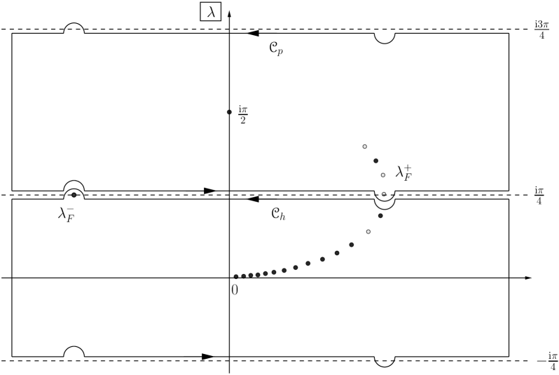
Figure 1: Sketch of the hole and particle contours ${\cal C}_{h}$ and ${\cal C}_{p}$. The Fermi rapidity $\lambda_{F}^{-}$ is located inside ${\cal C}_{h}$, while $\lambda_{F}^{+}$ lies inside ${\cal C}_{p}$.

The ‘hole contour’ ${\cal C}_{h}$ and the ‘particle contour’ ${\cal C}_{p}$ are sketched in Fig. 1. They are defined in such a way that ${\cal C}_{h}$ encloses all roots of ${\rm e}^{-\epsilon(x)/T}-1$ located inside the strip $-\pi/4<{\rm Im\,}x<\pi/4$ (‘the holes’) as well as the left Fermi rapidity $\lambda_{F}^{-}$, whereas ${\cal C}_{p}$ encloses the roots of ${\rm e}^{-\epsilon(x)/T}-1$ inside the strip $\pi/4<{\rm Im\,}x<3\pi/4$ (‘the particles’) as well as the right Fermi rapidity $\lambda_{F}^{+}$.

Given these contours we define the Cauchy transforms

$$\Phi_{h}(x)=\frac{{\rm i}p^{\prime}(x)}{2}\exp\biggl{\{}{\rm i}\int_{{\cal C}_{h}}{\rm d}\lambda\>p^{\prime}(\lambda)z(\lambda)\frac{\operatorname{sh}(x+\lambda)}{\operatorname{sh}(x-\lambda)}\biggr{\}}$$ (11)

for all $x\in{\cal S}\setminus{\cal C}_{h}$, and

$$\Phi_{p}(x)=\frac{{\rm i}p^{\prime}(x)}{2}\exp\biggl{\{}-{\rm i}\int_{{\cal C}_{p}}{\rm d}\lambda\>p^{\prime}(\lambda)z(\lambda)\frac{\operatorname{sh}(x+\lambda)}{\operatorname{sh}(x-\lambda)}\biggr{\}}$$ (12)

for all $x\in{\cal S}\setminus{\cal C}_{p}$. For fixed $x\in\operatorname{Int}({\cal C}_{h})\cup\operatorname{Int}({\cal C}_{p})$ the function $\operatorname{sh}(x+\lambda)/\operatorname{sh}(x-\lambda)$ is holomorphic in $\lambda$ for all $\lambda\in{\cal S}\setminus\bigl{(}\operatorname{Int}({\cal C}_{h})\cup\operatorname{Int}({\cal C}_{p})\bigr{)}$. Since the integrands in (11), (12) are rapidly decaying for $\lambda\rightarrow\pm\infty$, we may deform the contours and conclude that

$$\Phi_{h}(x)=\Phi_{p}(x)\quad\text{for all $x\in\operatorname{Int}({\cal C}_{h})\cup\operatorname{Int}({\cal C}_{p}$)}\,.$$ (13)

Another function needed below is the square of a generalized Cauchy determinant,

$${\cal D}\bigl{(}\{x_{j}\}_{j=1}^{m},\{y_{k}\}_{k=1}^{n}\bigr{)}=\frac{\bigl{[}\prod_{1\leq j<k\leq m}\operatorname{sh}^{2}(x_{j}-x_{k})\bigr{]}\bigl{[}\prod_{1\leq j<k\leq n}\operatorname{sh}^{2}(y_{j}-y_{k})\bigr{]}}{\prod_{j=1}^{m}\prod_{k=1}^{n}\operatorname{sh}^{2}(x_{j}-y_{k})}\,.$$ (14)

After these preparations we can now recall the form factor series derived in [9]. Using the above notation and performing several more or less obvious simplifications it can be written as

$$\bigl{\langle}\sigma_{1}^{-}\sigma_{m+1}^{+}(t)\bigr{\rangle}_{T}=(-1)^{m}{\cal F}(m)\sum_{n=1}^{\infty}\frac{(-1)^{n}}{n!(n-1)!}\prod_{j=1}^{n}\int_{{\cal C}_{h}}\frac{{\rm d}x_{j}}{\pi{\rm i}}\frac{\Phi_{p}(x_{j}){\rm e}^{{\rm i}(mp(x_{j})-t\epsilon(x_{j}))}}{1-{\rm e}^{\epsilon(x_{j})/T}}\\ \times\prod_{k=1}^{n-1}\int_{{\cal C}_{p}}\frac{{\rm d}y_{k}}{\pi{\rm i}}\frac{{\rm e}^{-{\rm i}(mp(y_{k})-t\epsilon(y_{k}))}}{\Phi_{h}(y_{k})\bigl{(}1-{\rm e}^{-\epsilon(y_{k})/T}\bigr{)}}\>{\cal D}\bigl{(}\{x_{j}\}_{j=1}^{n},\{y_{k}\}_{k=1}^{n-1}\bigr{)}\,,$$ (15)

where

$${\cal F}(m)={\rm e}^{-{\rm i}mp_{F}}\exp\biggl{\{}-\int_{{\cal C}_{h}^{\prime}\subset{\cal C}_{h}}{\rm d}\lambda\>z(\lambda)\int_{{\cal C}_{h}}{\rm d}\mu\>\operatorname{cth}^{\prime}(\lambda-\mu)z(\mu)\biggr{\}}\\ \times\exp\biggl{\{}-m\int_{{\cal C}_{h}}\frac{{\rm d}\lambda}{2\pi}p^{\prime}(\lambda)\ln\biggl{|}\operatorname{cth}\biggl{(}\frac{\epsilon(\lambda)}{2T}\biggr{)}\biggr{|}\biggr{\}}\,.$$ (16)

The contour ${\cal C}_{h}^{\prime}$ is tightly enclosed by ${\cal C}_{h}$.

3 Asymptotics in the spacelike regime

Theorem.

In the spacelike regime $m>4Jt$ the form factor series (15) is absolutely convergent and determines the late-time, large-distance asymptotics of the transverse dynamical correlation function of the XX chain as

$$\bigl{\langle}\sigma_{1}^{-}\sigma_{m+1}^{+}(t)\bigr{\rangle}_{T}=C(T,h)(-1)^{m}\exp\biggl{\{}-m\int_{{\cal C}_{h}}\frac{{\rm d}\lambda}{2\pi}p^{\prime}(\lambda)\ln\biggl{|}\operatorname{cth}\biggl{(}\frac{\epsilon(\lambda)}{2T}\biggr{)}\biggr{|}\biggr{\}}\\[4.30554pt] \times\bigl{(}1+{\cal O}(t^{-\infty})\bigr{)}\,,$$ (17)

where

$$C(T,h)=\frac{2T\Phi_{p}(\lambda_{F}^{-})}{\epsilon^{\prime}(\lambda_{F}^{-})}\exp\biggl{\{}-\int_{{\cal C}_{h}^{\prime}\subset{\cal C}_{h}}{\rm d}\lambda\>z(\lambda)\int_{{\cal C}_{h}}{\rm d}\mu\>\operatorname{cth}^{\prime}(\lambda-\mu)z(\mu)\biggr{\}}\,.$$ (18)

In preparation of the proof we introduce the short-hand notations

$$\tau=4Jt\,,\quad\alpha=\frac{m}{\tau}$$ (19)

and the function

$$g(\lambda)={\rm i}\bigl{(}\alpha p(\lambda)+\cos(p(\lambda))\bigr{)}$$ (20)

with real and imaginary parts $u(\lambda)={\rm Re\,}g(\lambda)$ and $v(\lambda)={\rm Im\,}g(\lambda)$. Then the ‘wave factors’ in (15) take the form

$${\rm e}^{\pm{\rm i}(mp(\lambda)-t\epsilon(\lambda))}={\rm e}^{\mp{\rm i}ht\pm\tau g(\lambda)}\,.$$ (21)

We will be interested in the asymptotic behaviour of (15) for large positive $\tau$ and fixed $\alpha>1$. As we shall see below, it is determined by the poles of the integrands at $\lambda_{F}^{\pm}$. The saddle points contribute only to the subleading corrections. This becomes clear when we consider the function $g$ close to the lines ${\mathbb{R}}\pm{\rm i}\pi/4$ and on the lines ${\rm Re\,}\lambda=\pm R$ for $R>0$ large enough.

Lemma.

Fix $\alpha>1$.

1. Then $g^{\prime}(\lambda)\neq 0$ for all $\lambda\in{\mathbb{R}}\pm{\rm i}\pi/4\mod{\rm i}\pi$, i.e. there are no saddle points on these lines.

2. Define the oriented contours

   $${\cal C}_{h,{\rm sd}}=\Bigl{[}-R+\frac{\pi{\rm i}}{4}-{\rm i}\delta,-R-\frac{\pi{\rm i}}{4}+{\rm i}\delta\Bigr{]}\cup\Bigl{[}-R-\frac{\pi{\rm i}}{4}+{\rm i}\delta,R-\frac{\pi{\rm i}}{4}+{\rm i}\delta\Bigr{]}$$

   $$\mspace{69.0mu}\cup\Bigl{[}R-\frac{\pi{\rm i}}{4}+{\rm i}\delta,R+\frac{\pi{\rm i}}{4}-{\rm i}\delta\Bigr{]}\cup\Bigl{[}R+\frac{\pi{\rm i}}{4}-{\rm i}\delta,-R+\frac{\pi{\rm i}}{4}-{\rm i}\delta\Bigr{]}\,,$$

   $${\cal C}_{p,{\rm sd}}={\cal C}_{h,{\rm sd}}+\frac{\pi{\rm i}}{2}\,,$$ (22)

   where $R,\delta>0$. Then $R$ and $\delta$ can be chosen in such a way that $u(\lambda)<0$ for all $\lambda\in{\cal C}_{h,{\rm sd}}$, $u(\lambda)>0$ for all $\lambda\in{\cal C}_{p,{\rm sd}}$ and all hole roots are inside ${\cal C}_{h,{\rm sd}}$, while all particle roots are inside ${\cal C}_{p,{\rm sd}}$.

Proof.

(i) For all $\alpha>1$ and $\lambda\in{\mathbb{R}}\pm{\rm i}\pi/4$ we have

$$g^{\prime}(\lambda)={\rm i}p^{\prime}(\lambda)\bigl{(}\alpha-\sin(p(\lambda))\bigr{)}\neq 0\,,$$ (23)

since

$${\rm i}p^{\prime}(\lambda)=\frac{2}{\operatorname{sh}(2\lambda)}\neq 0$$ (24)

for all $\lambda\in{\cal S}$, and $p(\lambda)\in{\mathbb{R}}$ for all $\lambda\in{\mathbb{R}}\pm{\rm i}\pi/4$ (see (9)).

(ii) Let $x={\rm Re\,}\lambda$, $y={\rm Im\,}\lambda$. Due to (23), (24) and the Cauchy-Riemann equations

$$\partial_{y}u(\lambda)=-{\rm Im\,}g^{\prime}(\lambda)=\pm\frac{2}{\operatorname{ch}(2x)}\bigl{(}\alpha-\sin(p(x\pm{\rm i}\pi/4))\bigr{)}$$ (25)

for $\lambda=x\pm{\rm i}\pi/4$. Now $\alpha>1$ by assumption. Thus, (25) implies that

$$\partial_{y}u(\lambda)\begin{cases}>0&\text{for $\lambda\in{\mathbb{R}}+{\rm i}\pi/4$}\\ <0&\text{for $\lambda\in{\mathbb{R}}-{\rm i}\pi/4$.}\end{cases}$$ (26)

Since $u=0$ for $\lambda\in{\mathbb{R}}\pm{\rm i}\pi/4$ it follows that $u(\lambda)<0$ on the lines $\lambda\in{\mathbb{R}}\pm{\rm i}\pi/4\mp{\rm i}\delta$ for small enough positive $\delta$. Similarly, $u(\lambda)>0$ on the lines ${\mathbb{R}}+{\rm i}\pi/4+{\rm i}\delta$ and ${\mathbb{R}}+3{\rm i}\pi/4-{\rm i}\delta$.

Since $\alpha>1$, there is a unique $\varphi>0$ such that $\alpha=\operatorname{cth}(2\varphi)$. Using this parameterization we find for any $\lambda=x+{\rm i}y\in{\cal S}$ that

$$\partial_{y}u(\lambda)=\frac{4}{\operatorname{sh}(2\varphi)|\operatorname{ch}(4\lambda)-1|^{2}}\bigl{[}\operatorname{sh}(4x)\operatorname{sh}(2(x+\varphi))\cos(2y)\sin(4y)\\ -(\operatorname{ch}(4x)\cos(4y)-1)\operatorname{ch}(2(x+\varphi))\sin(2y)\bigr{]}\,.$$ (27)

Thus, $\partial_{y}u(\lambda)=0$ if and only if

$$\sin(2y)\operatorname{ch}(2(x-\varphi))\biggl{[}\frac{\operatorname{sh}(4x)\operatorname{sh}(2(x+\varphi))+\operatorname{ch}(2(x+\varphi))}{\operatorname{ch}(2(x-\varphi))}-\cos(4y)\biggr{]}=0\,.$$ (28)

Here the first term in the square bracket is unbounded from above for $x\rightarrow\pm\infty$, implying that the only roots of $\partial_{y}u(\lambda)$ in $\cal S$ are at $y=0,\pi/2$ if $|x|$ is large enough. Taking into account (26) we see that, if the latter is the case, then

$$\partial_{y}u(\lambda)\begin{cases}>0&\text{for $y\in(0,\pi/2)$}\\ <0&\text{for $y\in(-\pi/4,0)\cup(\pi/2,3\pi/4)$.}\end{cases}$$ (29)

It follows that $u(\lambda)<0$ of the lines $\pm R+{\rm i}(-\pi/4,\pi/4)$, while $u(\lambda)>0$ on $\pm R+{\rm i}(\pi/4,3\pi/4)$, if $R>0$ large enough. The statement about the location of the particle and hole roots follows by straightforward inspection of the integrands in (15). ∎

Proof of the Theorem.

The function ${\cal D}\bigl{(}\{x_{j}\}_{j=1}^{n},\{y_{k}\}_{k=1}^{n-1}\bigr{)}$ is symmetric separately in all $x_{j}$ and $y_{k}$. It satisfies

$${\cal D}\bigl{(}\{x_{j}\}_{j=1}^{n},\{y_{k}\}_{k=1}^{n-1}\bigr{)}=0$$ (30)

if $x_{j}=x_{k}$ or $y_{j}=y_{k}$ for all $j\neq k$. Setting

$$V_{h}(x)=\frac{\Phi_{p}(x){\rm e}^{{\rm i}(mp(x)-t\epsilon(x))}}{\pi{\rm i}\bigl{(}{\rm e}^{\epsilon(x)/T}-1\bigr{)}}\,,\quad V_{p}(x)=\frac{{\rm e}^{-{\rm i}(mp(y)-t\epsilon(y))}}{\pi{\rm i}\Phi_{h}(y)\bigl{(}1-{\rm e}^{-\epsilon(y)/T}\bigr{)}}$$ (31)

and using the above lemma we therefore obtain

$$\bigl{\langle}\sigma_{1}^{-}\sigma_{m+1}^{+}(t)\bigr{\rangle}_{T}=(-1)^{m}{\cal F}(m)\sum_{n=1}^{\infty}\frac{1}{n!(n-1)!}\int_{{\cal C}_{h}^{n}}{\rm d}^{n}x\>\biggl{[}\prod_{j=1}^{n}V_{h}(x_{j})\biggr{]}$$

$$\mspace{180.0mu}\times\int_{{\cal C}_{p}^{n-1}}{\rm d}^{n-1}y\>\biggl{[}\prod_{k=1}^{n-1}V_{p}(y_{k})\biggr{]}{\cal D}\bigl{(}\{x_{j}\}_{j=1}^{n},\{y_{k}\}_{k=1}^{n-1}\bigr{)}$$

$$\mspace{18.0mu}=(-1)^{m}{\cal F}(m)\sum_{n=1}^{\infty}\frac{1}{n!(n-1)!}\biggl{(}\int_{{\cal C}_{h,{\rm sd}}^{n}}{\rm d}^{n}x\>\prod_{j=1}^{n}V_{h}(x_{j})$$

$$\mspace{162.0mu}+n\int_{{\cal C}_{h,{\rm sd}}^{n-1}}{\rm d}^{n-1}x\>\biggl{[}\prod_{j=1}^{n-1}V_{h}(x_{j})\biggr{]}2\pi{\rm i}\operatorname{res}\bigl{\{}{\rm d}x_{n}\>V_{h}(x_{n}),x_{n}=\lambda_{F}^{-}\bigr{\}}\biggr{)}$$

$$\mspace{45.0mu}\times\biggl{(}\int_{{\cal C}_{p,{\rm sd}}^{n-1}}{\rm d}^{n-1}y\>\prod_{k=1}^{n-1}V_{p}(y_{k})$$

$$\mspace{72.0mu}+(n-1)\int_{{\cal C}_{p,{\rm sd}}^{n-2}}{\rm d}^{n-2}y\>\biggl{[}\prod_{k=1}^{n-2}V_{p}(y_{k})\biggr{]}2\pi{\rm i}\operatorname{res}\bigl{\{}{\rm d}y_{n-1}\>V_{p}(y_{n-1}),y_{n-1}=\lambda_{F}^{+}\bigr{\}}\biggr{)}$$

$$\mspace{360.0mu}\times{\cal D}\bigl{(}\{x_{j}\}_{j=1}^{n},\{y_{k}\}_{k=1}^{n-1}\bigr{)}\,.$$ (32)

Here ${\cal C}_{h,{\rm sd}}$ and ${\cal C}_{p,{\rm sd}}$ are the contours introduced in (2). Notice that we consider $\operatorname{res}\bigl{\{}{\rm d}x\>V_{h}(x),x=\lambda_{F}^{-}\bigr{\}}$ as a functional acting on functions $f$ holomorphic in a disc $D_{\varepsilon}(\lambda_{F}^{-})$ of sufficiently small radius $\varepsilon$ centered about $\lambda_{F}^{-}$ as

$$\operatorname{res}\bigl{\{}{\rm d}x\>V_{h}(x),x=\lambda_{F}^{-}\bigr{\}}f=\int_{D_{\varepsilon}(\lambda_{F}^{-})}\frac{{\rm d}x}{2\pi{\rm i}}\>V_{h}(x)f(x)\,,$$ (33)

and similarly for $\operatorname{res}\bigl{\{}{\rm d}y\>V_{p}(y),y=\lambda_{F}^{+}\bigr{\}}$. In particular,

$$2\pi{\rm i}\operatorname{res}\bigl{\{}{\rm d}x\>V_{h}(x),x=\lambda_{F}^{-}\bigr{\}}1=\frac{2T{\rm e}^{{\rm i}mp_{F}}\Phi_{p}(\lambda_{F}^{-})}{\epsilon^{\prime}(\lambda_{F}^{-})}\,,$$ (34a)

$$2\pi{\rm i}\operatorname{res}\bigl{\{}{\rm d}y\>V_{p}(y),y=\lambda_{F}^{+}\bigr{\}}1=\frac{2T{\rm e}^{{\rm i}mp_{F}}}{\Phi_{h}(\lambda_{F}^{+})\epsilon^{\prime}(\lambda_{F}^{+})}\,.$$ (34b)

Equation (3) implies that

$$\bigl{\langle}\sigma_{1}^{-}\sigma_{m+1}^{+}(t)\bigr{\rangle}_{T}=(-1)^{m}{\cal F}(m)\sum_{\ell=1}^{4}S_{\ell}(m,t)\,,$$ (35)

where the four series $S_{\ell}(m,t)$ can be written as follows.

$$S_{1}(m,t)=\frac{2T{\rm e}^{{\rm i}mp_{F}}\Phi_{p}(\lambda_{F}^{-})}{\epsilon^{\prime}(\lambda_{F}^{-})}\sum_{n=0}^{\infty}S_{1}^{(n)}(m,t)\,,$$ (36a)

$$S_{2}(m,t)=-\frac{1}{\operatorname{sh}^{2}(\lambda_{F}^{+}-\lambda_{F}^{-})}\biggl{(}\frac{2T{\rm e}^{{\rm i}mp_{F}}}{\epsilon^{\prime}(\lambda_{F}^{-})}\biggr{)}^{2}\frac{\Phi_{p}(\lambda_{F}^{-})}{\Phi_{h}(\lambda_{F}^{+})}\sum_{n=0}^{\infty}S_{2}^{(n)}(m,t)\,,$$ (36b)

$$S_{3}(m,t)=\frac{2T{\rm e}^{{\rm i}mp_{F}}}{\Phi_{h}(\lambda_{F}^{+})\epsilon^{\prime}(\lambda_{F}^{-})}\sum_{n=0}^{\infty}S_{3}^{(n)}(m,t)\,,$$ (36c)

$$S_{4}(m,t)=\sum_{n=0}^{\infty}S_{4}^{(n)}(m,t)$$ (36d)

with

$$S_{1}^{(n)}(m,t)=\frac{1}{(n!)^{2}}\int_{{\cal C}_{h,{\rm sd}}^{n}}\mspace{-18.0mu}{\rm d}^{n}x\>\biggl{[}\prod_{j=1}^{n}V_{h}(x_{j})\biggr{]}\int_{{\cal C}_{p,{\rm sd}}^{n}}\mspace{-18.0mu}{\rm d}^{n}y\>\biggl{[}\prod_{k=1}^{n}V_{p}(y_{k})\biggr{]}$$

$$\mspace{180.0mu}\times\biggl{[}\prod_{j=1}^{n}\frac{\operatorname{sh}^{2}(x_{j}-\lambda_{F}^{-})}{\operatorname{sh}^{2}(y_{j}-\lambda_{F}^{-})}\biggr{]}{\cal D}\bigl{(}\{x_{j}\}_{j=1}^{n},\{y_{k}\}_{k=1}^{n}\bigr{)}\,,$$ (37a)

$$S_{2}^{(n)}(m,t)=\frac{1}{(n+1)!n!}\int_{{\cal C}_{h,{\rm sd}}^{n+1}}\mspace{-18.0mu}{\rm d}^{n+1}x\>\biggl{[}\prod_{j=1}^{n+1}V_{h}(x_{j})\frac{\operatorname{sh}^{2}(x_{j}-\lambda_{F}^{-})}{\operatorname{sh}^{2}(x_{j}-\lambda_{F}^{+})}\biggr{]}$$

$$\mspace{18.0mu}\times\int_{{\cal C}_{p,{\rm sd}}^{n}}\mspace{-18.0mu}{\rm d}^{n}y\>\biggl{[}\prod_{k=1}^{n}V_{p}(y_{k})\frac{\operatorname{sh}^{2}(y_{k}-\lambda_{F}^{+})}{\operatorname{sh}^{2}(y_{k}-\lambda_{F}^{-})}\biggr{]}\biggl{[}\prod_{j=1}^{n}\frac{\operatorname{sh}^{2}(x_{j}-x_{n+1})}{\operatorname{sh}^{2}(y_{j}-x_{n+1})}\biggr{]}{\cal D}\bigl{(}\{x_{j}\}_{j=1}^{n},\{y_{k}\}_{k=1}^{n}\bigr{)}\,,$$ (37b)

$$S_{3}^{(n)}(m,t)=-\frac{1}{(n+2)!n!}\int_{{\cal C}_{h,{\rm sd}}^{n+2}}\mspace{-18.0mu}{\rm d}^{n+2}x\>\biggl{[}\prod_{j=1}^{n+2}\frac{V_{h}(x_{j})}{\operatorname{sh}^{2}(x_{j}-\lambda_{F}^{+})}\biggr{]}\operatorname{sh}^{2}(x_{n+1}-x_{n+2})$$

$$\times\int_{{\cal C}_{p,{\rm sd}}^{n}}\mspace{-20.0mu}{\rm d}^{n}y\>\biggl{[}\prod_{k=1}^{n}V_{p}(y_{k})\operatorname{sh}^{2}(y_{k}-\lambda_{F}^{+})\biggr{]}\biggl{[}\prod_{j=1}^{n}\prod_{k=1}^{2}\frac{\operatorname{sh}^{2}(x_{j}-x_{n+k})}{\operatorname{sh}^{2}(y_{j}-x_{n+k})}\biggr{]}{\cal D}\bigl{(}\{x_{j}\}_{j=1}^{n},\{y_{k}\}_{k=1}^{n}\bigr{)},$$ (37c)

$$S_{4}^{(n)}(m,t)=\frac{1}{(n+1)!n!}\int_{{\cal C}_{h,{\rm sd}}^{n+1}}\mspace{-18.0mu}{\rm d}^{n+1}x\>\biggl{[}\prod_{j=1}^{n+1}V_{h}(x_{j})\biggr{]}\int_{{\cal C}_{p,{\rm sd}}^{n}}\mspace{-18.0mu}{\rm d}^{n}y\>\biggl{[}\prod_{k=1}^{n}V_{p}(y_{k})\biggr{]}$$

$$\mspace{180.0mu}\times\biggl{[}\prod_{j=1}^{n}\frac{\operatorname{sh}^{2}(x_{j}-x_{n+1})}{\operatorname{sh}^{2}(y_{j}-x_{n+1})}\biggr{]}{\cal D}\bigl{(}\{x_{j}\}_{j=1}^{n},\{y_{k}\}_{k=1}^{n}\bigr{)}\,.$$ (37d)

In order to show the convergence of the series and to estimate their asymptotic behaviour, we have to establish bounds on the individual terms. We start with the functions ${\cal D}\bigl{(}\{x_{j}\}_{j=1}^{n},\{y_{k}\}_{k=1}^{n}\bigr{)}$ and recall the Hadamard bound for the determinant of an $n\times n$ matrix

$$\Bigl{|}\det_{j,k=1,\dots,n}(M_{jk})\Bigr{|}\leq\Bigl{(}\max_{j,k=1,\dots,n}|M_{jk}|\Bigr{)}^{n}\cdot n^{\frac{n}{2}}\,.$$ (38)

Since the contours ${\cal C}_{h,{\rm sd}}$ and ${\cal C}_{p,{\rm sd}}$ are finite and disjoint, we can use (38) to estimate

$$\Bigl{|}{\cal D}\bigl{(}\{x_{j}\}_{j=1}^{n},\{y_{k}\}_{k=1}^{n}\bigr{)}\Bigr{|}=\biggl{|}\det_{j,k=1,\dots,n}\biggl{(}\frac{1}{\operatorname{sh}(x_{j}-y_{k})}\biggr{)}\biggr{|}^{2}\leq B^{2n}n^{n}\,,$$ (39)

where

$$B=\sup_{\begin{subarray}{c}x\in{\cal C}_{h,{\rm sd}}\\ y\in{\cal C}_{p,{\rm sd}}\end{subarray}}\biggl{|}\frac{1}{\operatorname{sh}(x-y)}\biggr{|}\,.$$ (40)

Likewise we set

$$C=\sup_{\begin{subarray}{c}x\in{\cal C}_{h,{\rm sd}}\\ y\in{\cal C}_{p,{\rm sd}}\end{subarray}}\biggl{|}\frac{\operatorname{sh}(x-\lambda_{F}^{-})}{\operatorname{sh}(y-\lambda_{F}^{-})}\biggr{|}\,.$$ (41)

As follows from the above lemma, there exist $\kappa,c>0$ such that

$$\sup_{\begin{subarray}{c}x\in{\cal C}_{h,{\rm sd}}\\ y\in{\cal C}_{p,{\rm sd}}\end{subarray}}\bigl{(}\max\bigl{\{}|V_{h}(x)|,|V_{p}(y)|\bigr{\}}\bigr{)}=\kappa{\rm e}^{-\tau c}\,.$$ (42)

With this we obtain a bound on every individual term in the series $S_{1}$,

$$|S_{1}^{(n)}(m,t)|\leq\frac{1}{(n!)^{2}}\bigl{(}|{\cal C}_{h,{\rm sd}}||{\cal C}_{p,{\rm sd}}|\bigr{)}^{n}C^{2n}\kappa^{2n}{\rm e}^{-2n\tau c}B^{2n}n^{n}\leq\frac{1}{n!}C_{1}^{n}{\rm e}^{-2n\tau c}$$ (43)

for some constant $C_{1}>0$. This implies absolute convergence of the series $S_{1}$ and shows that, asymptotically for large $\tau$, the series behaves like

$$S_{1}(m,t)=\frac{2T{\rm e}^{{\rm i}mp_{F}}\Phi_{p}(\lambda_{F}^{-})}{\epsilon^{\prime}(\lambda_{F}^{-})}\bigl{(}1+{\cal O}({\rm e}^{-2\tau c})\bigr{)}\,.$$ (44)

In a similar way one obtains

$$|S_{2}^{(n)}(m,t)|\leq\frac{1}{n!}C_{2}^{n}{\rm e}^{-(2n+1)\tau c}\,,$$ (45a)

$$|S_{3}^{(n)}(m,t)|\leq\frac{1}{n!}C_{3}^{n}{\rm e}^{-(2n+2)\tau c}\,,$$ (45b)

$$|S_{4}^{(n)}(m,t)|\leq\frac{1}{n!}C_{4}^{n}{\rm e}^{-(2n+1)\tau c}\,,$$ (45c)

for constants $C_{j}>0$, $j=2,3,4$. It follows that the series $S_{j}$, $j=2,3,4$, converge absolutely and behave asymptotically as

$$S_{2}(m,t)={\cal O}({\rm e}^{-\tau c})\,,$$ (46a)

$$S_{3}(m,t)={\cal O}({\rm e}^{-2\tau c})\,,$$ (46b)

$$S_{4}(m,t)={\cal O}({\rm e}^{-\tau c})\,.$$ (46c)

Inserting (44), (46) into (35) and recalling the explicit form (16) of ${\cal F}(m)$ we have arrived at the statement of the theorem. ∎

The theorem fixes the constant term of the asymptotics in the spacelike regime that remained undetermined in [12]. Note that the function $\epsilon^{\prime}(\lambda_{F}^{-})$ can be easily calculated explicitly,

$$\epsilon^{\prime}(\lambda_{F}^{-})=-2h\sqrt{1-\Bigl{(}\frac{h}{4J}\Bigr{)}^{2}}\,.$$ (47)

For the other factors composing the constant $C(T,h)$ we did not find any further simplification so far.

4 Discussion

For the interpretation of our result we would like to recall a Fredholm determinant representation of the transversal two-point function (2) that was obtained in [11], where it was used for the asymptotic analysis of the correlation function in the high-temperature limit. Referring to [11] we define the functions

$$\varphi(x,y)=\frac{{\rm e}^{y-x}}{\operatorname{sh}(y-x)}$$ (48)

and

$$\Omega=\int_{{\cal C}_{h}}{\rm d}x\>V_{h}(x)\,,$$ (49a)

$$E_{h}(x)=\int_{{\cal C}_{h}}{\rm d}y\>V_{h}(y)\varphi(y,x)\,,$$ (49b)

$$V(x,y)=\int_{{\cal C}_{h}}{\rm d}z\>V_{h}(z)\varphi(z,x)\varphi(z,y)\,.$$ (49c)

Using these functions we define two integral operators $\widehat{V}$ and $\widehat{P}$ acting on functions on the contour ${\cal C}_{p}$,

$$\widehat{V}f(x) =\int_{{\cal C}_{p}}{\rm d}y\>V_{p}(y)V(x,y)f(y)\,,$$ (50a)

$$\widehat{P}f(x) =\frac{E_{h}(x)}{\Omega}\int_{{\cal C}_{p}}{\rm d}y\>V_{p}(y)E_{h}(y)f(y)\,.$$ (50b)

Then (cf. [11]) the transversal correlation functions of the XX chain admit the Fredholm determinant representation

$$\bigl{\langle}\sigma_{1}^{-}\sigma_{m+1}^{+}(t)\bigr{\rangle}_{T}=(-1)^{m}{\cal F}(m)\Omega(m,t)\det_{{\cal C}_{p}}\bigl{(}\operatorname{id}+\widehat{V}-\widehat{P}\bigr{)}\,.$$ (51)

Comparing with the asymptotic behaviour of the correlation function in the spacelike regime $m>4Jt$ we see that

$$\det_{{\cal C}_{p}}\bigl{(}\operatorname{id}+\widehat{V}-\widehat{P}\bigr{)}\sim 1+{\cal O}(t^{-\infty})\,,$$ (52)

meaning that the Fredholm determinant collects the higher-order corrections to the main asymptotics. This is the analogy with the Borodin-Okounkov-Geronimo-Case formula [3, 8] mentioned in the introduction.

On the level of the Fredholm determinant representation it is easiest to compare our result with that of Its, Izergin, Korepin and Slavnov [12]. For this purpose we rewrite their integral operators acting on functions on the the unit circle as integral operators acting on functions on ${\cal C}=[-\infty-{\rm i}\pi/4,+\infty-{\rm i}\pi/4]\cup[+\infty+{\rm i}\pi/4,-\infty+{\rm i}\pi/4]$. This is achieved by employing the map $z\mapsto{\rm e}^{{\rm i}p(\lambda)}$ to the Fredholm determinant representation in [12]. Then

$$\bigl{\langle}\sigma_{1}^{-}\sigma_{m+1}^{+}(t)\bigr{\rangle}_{T}=(-1)^{m}\bigl{[}\det_{{\cal C}}\bigl{(}\operatorname{id}+\widehat{W}+\widehat{Q}\bigr{)}-\det_{{\cal C}}\bigl{(}\operatorname{id}+\widehat{W}\bigr{)}\bigr{]}\,,$$ (53)

where $\widehat{W}$ is an integrable operator with kernel

$$W(\lambda,\mu) =\frac{\operatorname{ch}(\lambda)H(\lambda)-\operatorname{ch}(\mu)H(\mu)}{\operatorname{sh}(\lambda-\mu)}\frac{{\rm e}^{{\rm i}(mp(\mu)-t\epsilon(\mu))}}{\pi(1+{\rm e}^{\epsilon(\mu)/T})}\,,$$ (54a)

$$H(\lambda) ={\rm v.p.}\int_{\cal C}\frac{{\rm d}\mu}{\pi}\frac{{\rm e}^{-{\rm i}(mp(\mu)-t\epsilon(\mu))}}{\operatorname{ch}(\mu)\operatorname{sh}(\mu-\lambda)}$$ (54b)

and $\widehat{Q}$ is a one-dimensional projector acting as

$$\widehat{Q}f(\lambda)=\frac{1}{\operatorname{ch}(\lambda)}\int_{\cal C}\frac{{\rm d}\mu}{2\pi{\rm i}}\frac{{\rm e}^{{\rm i}(mp(\mu)-t\epsilon(\mu))}f(\mu)}{\operatorname{sh}(\mu)(1+{\rm e}^{\epsilon(\mu)/T})}\,.$$ (55)

Comparing (51) and (53) we see that in (53) the late-time, large-distance asymptotics is entirely inside the Fredholm determinants and therefore harder to analyse.

The fact that the late-time, large-distance asymptotic behaviour of the transverse dynamical correlation functions of the XX chain, including the constant term, can be obtained directly from the series representation (15) raises a number of interesting questions.

1. Is a similar analysis possible for the XXZ quantum spin chain? Unlike the XX chain treated in this work no Fredholm determinant representation for its two-point function is expected to exist, but a thermal form-factor series similar to (15) is still available [9]. As the structure of the saddle-point equations is very similar, there seems to be a good chance that the answer will turn out to be positive.

2. What can be done in the timelike regime? Here all terms in the series (15) contribute to the late-time, large-distance asymptotics. A further resummation would be necessary. Can we devise a method to find such a generalization?

We would like to close with two remarks. First, in our recent work [10] we have compared the asymptotic formula of our theorem with a numerical evaluation based on the Fredholm determinant representation (51). As should be clear from the fact that the corrections are exponentially small for large $m$ and $t$ the asymptotic formula turns out to be very efficient. For an example see Fig. 2. Second, the constant term $C(t,h)$, equation (18), does not depend on $\alpha$. For this reason it should agree with the constant obtained by Barouch and McCoy [1] in form of infinite double products in their analysis of the static correlation functions (see equations (3.17)-(3.19) of their paper). We have numerical evidence that this is indeed the case.

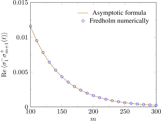
Figure 2: Real part of $\langle\sigma^{-}_{1}\sigma^{+}_{m+1}(t)\rangle$ as a function of $m$ for $T/J=0.05$, $h/J=0.1$ and $Jt=10$ evaluated numerically and from (17).

Acknowledgements. The authors would like to thank Alexander Its and Nikita Slavnov for helpful discussions. FG is supported by the Deutsche Forschungsgemeinschaft within the framework of the research unit FOR 2316 ‘Correlations in integrable quantum many-body systems’. The work of KKK is supported by the CNRS and by the ‘Projet international de coopération scientifique No. PICS07877’: Fonctions de corrélations dynamiques dans la chaîne XXZ à température finie, Allemagne, 2018-2020. JS is supported by JSPS KAKENHI Grants, numbers 18K03452 and 18H01141.

References

- [1] E. Barouch and B. M. McCoy, Statistical mechanics of the XY model. II. Spin correlation functions, Phys. Rev. A 3 (1971), 786–804.
- [2] E. L. Basor and H. Widom, On a Toeplitz determinant identity of Borodin and Okounkov, Integr. Equ. Oper. Theory 37 (2000), 397–401.
- [3] A. Borodin and A. Okounkov, A Fredholm determinant formula for Toeplitz determinants, Integr. Equ. Oper. Theory 37 (2000), 386–396.
- [4] U. Brandt and K. Jacoby, Exact results for the dynamics of one-dimensional spin-systems, Z. Phys. B 25 (1976), 181–187.
- [5] F. Colomo, A. G. Izergin, V. E. Korepin, and V. Tognetti, Temperature correlation functions in the XX0 Heisenberg chain. I, Theor. Math. Phys. 94 (1993), 11–38.
- [6] P. A. Deift and X. Zhou, A steepest descent method for oscillatory Riemann-Hilbert problems. Asymptotics for the MKdV equation, Ann. of Math. 137 (1993), 295–368.
- [7] M. Dugave, F. Göhmann, and K. K. Kozlowski, Thermal form factors of the XXZ chain and the large-distance asymptotics of its temperature dependent correlation functions, J. Stat. Mech.: Theor. Exp. (2013), P07010.
- [8] J. S. Geronimo and K. M. Case, Scattering theory and polynomials orthogonal on the unit circle, J. Math. Phys. 20 (1979), 299–310.
- [9] F. Göhmann, M. Karbach, A. Klümper, K. K. Kozlowski, and J. Suzuki, Thermal form-factor approach to dynamical correlation functions of integrable lattice models, J. Stat. Mech.: Theor. Exp. (2017), 113106.
- [10] F. Göhmann, K. K. Kozlowski, J. Sirker, and J. Suzuki, The equilibrium dynamics of the XX chain revisited, preprint, arXiv:1906.03143, 2019.
- [11] F. Göhmann, K. K. Kozlowski, and J. Suzuki, High-temperature analysis of the transverse dynamical two-point correlation function of the XX quantum-spin chain, preprint, arXive:1905.04922, 2019.
- [12] A. R. Its, A. G. Izergin, V. E. Korepin, and N. Slavnov, Temperature correlations of quantum spins, Phys. Rev. Lett. 70 (1993), 1704–1706.
- [13] X. Jie, The large time asymptotics of the temperature correlation functions of the XX0 Heisenberg ferromagnet: The Riemann-Hilbert approach, Ph.D. thesis, Indiana University Purdue University Indianapolis, 1998.
- [14] K. K. Kozlowski, Long-distance and large-time asymptotic behaviour of dynamic correlation functions in the massless regime of the XXZ spin-1/2 chain, preprint, arXiv:1903.00207, 2019.
- [15] E. H. Lieb, T. Schultz, and D. Mattis, Two soluble models of an antiferromagnetic chain, Ann. Phys. (N.Y.) 16 (1961), 407–466.
- [16] J. H. H. Perk and H. W. Capel, Time-dependent xx-correlation functions in the one-dimensional XY-model, Physica A 89 (1977), 265–303.