The average genus for bouquets of circles and dipoles

Abstract

The bouquet of circles $B_{n}$ and dipole graph $D_{n}$ are two important classes of graphs in topological graph theory. For $n\geqslant 1$, we give an explicit formula for the average genus $\gamma_{avg}(B_{n})$ of $B_{n}$. By this expression, one easily sees $\gamma_{avg}(B_{n})=\frac{n-\ln n-c+1-\ln 2}{2}+o(1)$, where $c$ is the Euler constant. Similar results are obtained for $D_{n}$. Our method is new and deeply depends on the knowledge in ordinary differential equations.
Keywords: Average genus; Bouquet of circles; Dipole; Ordinary differential equations
MSC 2000: 05C10

1 Introduction and Main Results

A graph $G=(V(G),E(G))$ is permitted to have both loops and multiple edges. A embedding of a graph $G$ into an orientable surface $O_{k}$ is a cellular embedding, i.e., the interior of every face is homeomorphic to an open disc. We denote the number of cellular embeddings of $G$ on the surface $O_{k}$ by $g_{k}(G)$, where, by the number of embeddings, we mean the number of equivalence classes under ambient isotopy. The genus polynomial of a graph $G$ is given by

$$\Gamma_{G}(x)=\sum_{k\geqslant 0}g_{k}(G)x^{k},$$

This sequence $\{g_{k}(G),k=0,1,2,\cdots,\}$ is called the genus distribution of the graph $G$.

The average genus $\gamma_{avg}(G)$ of the graph $G$ is the expected value of the genus random variable, over all labeled 2-cell orientable embeddings of $G$, using the uniform distribution. In other words, the average genus of $G$ is

$$\gamma_{avg}(G) = \frac{\Gamma_{G}^{\prime}(1)}{\Gamma_{G}(1)}=\sum_{k=0}^{\infty}k\cdot\frac{g_{k}(G)}{\Gamma_{G}(1)}.$$

The study of the average genus of a graph began by Gross and Furst [9], and much further developed by Chen and Gross [1, 2, 4]. Two lower bounds were obtained in [3] for the average genus of two kinds of graphs. In [18], Stahl gave the asymptotic result for average genus of linear graph families. The exact value for the average genus of small-order complete graphs, closed-end ladders, and cobblestone paths were derived by White [22]. More references are the following: [5, 11, 14, 16, 19] etc. For general background in topological graph theory, we refer the readers to see Gross and Tucker [8] or White [21].

One objective of this paper is to give an explicit expression of the average genus for a bouquet of circles. By a bouquet of circles, or more briefly, a bouquet, we mean a graph with one vertex and some self-loops. In particular, the bouquet with $n$ self-loops is denoted $B_{n}$. Figure 1 demonstrates the graphs $B_{1},B_{2},B_{3}.$ The bouquets $\{B_{n},n\geqslant 1\}$ are very important graphs in topological graph theory. First, since any connected graph can be reduced to a bouquet by contracting a spanning tree to a point, bouquets are fundamental building blocks of topological graph theory. Second, as that demonstrated in [6, 7], Cayley graphs and many other regular graphs are covering spaces of bouquets.

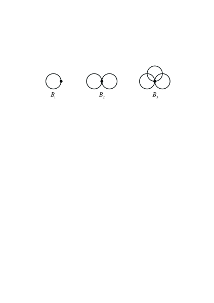
Figure 1: The bouquets $B_{1},B_{2},$ and $B_{3}.$

For the genus distribution of $B_{n}$, Gross, Robbins and Tucker [10] proved that the numbers $g_{m}(B_{n})$ of embeddings of the $B_{n}$ in the oriented surface of genus $m$ satisfy the following recurrence for $n>2,$

$$\begin{split}(n+1)g_{m}(B_{n})&=4(2n-1)(2n-3)(n-1)^{2}(n-2)g_{m-1}(B_{n-2})\\ &\quad+4(2n-1)(n-1)g_{m}(B_{n-1})\end{split}$$ (1.1)

with initial conditions

$$g_{m}(B_{0})=1\text{ for }m=0\text{ and }g_{m}(B_{0})=1\text{ for }m>0,$$

$$g_{m}(B_{1})=1\text{ for }m=0\text{ and }g_{m}(B_{1})=1\text{ for }m>0.$$

With an aid of edge-attaching surgery technique, the total embedding polynomials of $B_{n}$ was computed in [12]. Stahl [17] also did some researches on the average genus of $B_{n}$. By [17, Theorem 2.5] and Euler formula, one easily sees that

$$\lim_{n\rightarrow\infty}\Big{(}\gamma_{avg}(B_{n})-\big{(}\frac{n+1}{2}-\frac{1}{2}\sum_{k=1}^{2n}\frac{1}{k}\big{)}\Big{)}=0.$$ (1.2)

To achieve this, Stahl made many accurate estimates on the unsigned Stirling numbers $s(n,k)$ of the first kind. In this paper, using knowledge in ordinary differential equations and Taylor formulas, we derive an explicit expression of $\gamma_{avg}(B_{n}).$ By this expression, (1.2) follows immediately. Our methods are totally different from that in [17] and we don’t need to make estimates on $s(n,k)$. In Section 2, we will give the computation of $\gamma_{avg}(B_{n})$ in detail.

Another objective of this paper is to give an explicit expression of the average genus for dipoles $D_{n}$ (two vertices, $n-$multiple edges). Figure 2 demonstrates the graphs $D_{1},D_{2},D_{3}.$

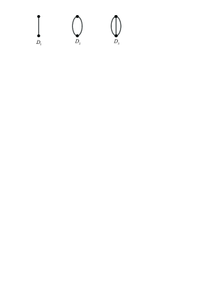
Figure 2: The dipoles $D_{1},D_{2},$ and $D_{3}.$

The dipole, like the bouquet, is useful as a voltage graph. See [21] for example. Moreover, hypermaps correspond with the 2-cell embeddings of the dipole. The genus distributions of $D_{n}$ are given by [12] and [15]. In this paper, the calculation of $\gamma_{avg}(D_{n})$ are similar as that in $\gamma_{avg}(B_{n}).$ But the processes are more complicated, so we still give their details in Section 3.

It is not difficult to obtain the following recurrence relation for $\gamma_{avg}(B_{n})$

$$\gamma_{avg}(B_{n}) = \frac{2}{n+1}\gamma_{avg}(B_{n-1})+\frac{n-1}{n+1}\big{(}\gamma_{avg}(B_{n-2})+1\big{)}.$$

Since the coefficients before $\gamma_{avg}(B_{n-2})$ and $\gamma_{avg}(B_{n-1})$ depend on $n$, there are little tools to obtain the explicit expression of $\gamma_{avg}(B_{n})$. In this paper, we give a method to get explicit expression of $\gamma_{avg}(B_{n})$. Our method is new and deeply depends on the knowledge in ordinary differential equations and series theory.

2 The average genus of $B_{n}$

The main objective of this section is to prove the following theorem.

Theorem 2.1.

The average genus of $B_{n}$ is given by

$$\gamma_{avg}(B_{n})=\frac{n+1}{2}-\sum_{m=0}^{n-1}\frac{1+(-1)^{m}}{2(m+1)}-\frac{1+(-1)^{n}}{4(n+1)}.$$

In particular, we have

$$\gamma_{avg}(B_{n})=\frac{n-\ln n-c+1-\ln 2}{2}+o(1),$$

where $c\approx 0.5772$ is the Euler constant.

Proof.

Multiplying both sides of (1.1) by $x^{m}$, it holds that

$$\begin{split}\sum_{m\geqslant 0}(n+1)g_{m}(B_{n})x^{m}&=\sum_{m\geqslant 0}4(2n-1)(2n-3)(n-1)^{2}(n-2)g_{m-1}(B_{n-2})x^{m}\\ &\quad+\sum_{m\geqslant 0}4(2n-1)(n-1)g_{m}(B_{n-1})x^{m}.\end{split}$$ (2.1)

Hence, the genus polynomial $\Gamma_{B_{n}}(x)$ satisfy the following recurrence

$$\begin{split}(n+1)\Gamma_{B_{n}}(x)&=4(2n-1)(2n-3)(n-1)^{2}(n-2)\cdot x\cdot\Gamma_{B_{n-2}}(x)\\ &\quad+4(2n-1)(n-1)\Gamma_{B_{n-1}}(x)\end{split}$$ (2.2)

with initial conditions $\Gamma_{B_{1}}(x)=1,\Gamma_{B_{2}}(x)=4+2x.$

By (2.2), we have

$$(n+1)\Gamma_{B_{n}}^{\prime}(1)=4(2n-1)(2n-3)(n-1)^{2}(n-2)\cdot\Gamma_{B_{n-2}}^{\prime}(1)$$

$$~{}~{}~{}+4(2n-1)(2n-3)(n-1)^{2}(n-2)\cdot\Gamma_{B_{n-2}}(1)+4(2n-1)(n-1)\Gamma_{B_{n-1}}^{\prime}(1).$$

Dividing both sides of the above equality by $\Gamma_{B_{n}}(1)=(2n-1)!$, for $n\geqslant 3,$ one arrives at that

$$(n+1)\gamma_{avg}(B_{n})\! = \!2\gamma_{avg}(B_{n-1})+(n-1)\big{(}\gamma_{avg}(B_{n-2})+1\big{)}.$$ (2.3)

By direct calculation, one sees $\gamma_{avg}(B_{1})=0,\gamma_{avg}(B_{2})=\frac{1}{3}.$ For $n\leqslant 0$, we define $\gamma_{avg}(B_{n})=0$ so that (2.3) holds for any integer $n\geqslant 1.$ For simplicity of writing, we use $a_{n}$ to denote $\gamma_{avg}(B_{n})$ in the rest of proof. Thus, $a_{n}$ satisfies the following recurrence relation

$$a_{n}=\frac{2}{n+1}a_{n-1}+\frac{n-1}{n+1}(a_{n-2}+1)$$ (2.4)

with initial conditions $a_{1}=0,a_{2}=\frac{1}{3}.$

Using $(\ref{1-1})$, we have

$$(n+1)a_{n}=2a_{n-1}+(n-1)(a_{n-2}+1)$$

and

$$\sum_{n\geqslant 1}(n+1)a_{n}t^{n}=2\sum_{n\geqslant 1}a_{n-1}t^{n}+\sum_{n\geqslant 1}(n-1)(a_{n-2}+1)t^{n}.$$ (2.5)

Let $u(t)=\sum_{n\geqslant 1}a_{n}t^{n}.$ Then, by (2.5), we obtain

$$\Big{(}t\cdot\sum_{n\geqslant 1}a_{n}t^{n}\Big{)}^{\prime} = 2t\cdot\sum_{n\geqslant 1}a_{n-1}t^{n-1}+\sum_{n\geqslant 1}(n-2)a_{n-2}t^{n}+\sum_{n\geqslant 1}a_{n-2}t^{n}+\sum_{n\geqslant 1}(n-1)t^{n}$$

$$= 2tu(t)+t^{3}\sum_{n\geqslant 1}(n-2)a_{n-2}t^{n-3}+t^{2}u(t)+t^{2}\cdot(\sum_{n\geqslant 2}t^{n-1})^{\prime},$$

that is

$$(tu(t))^{\prime} = 2tu(t)+t^{3}\sum_{n\geqslant 3}(n-2)a_{n-2}t^{n-3}+t^{2}u(t)+t^{2}\Big{(}\frac{t}{1-t}\Big{)}^{\prime}$$

$$= 2tu(t)+t^{3}\sum_{n\geqslant 1}na_{n}t^{n-1}+t^{2}u(t)+t^{2}\Big{(}\frac{t}{1-t}\Big{)}^{\prime}$$

$$= 2tu(t)+t^{3}u^{\prime}(t)+t^{2}u(t)+t^{2}\Big{(}\frac{t}{1-t}\Big{)}^{\prime},$$

which implies that $u(t)$ satisfies the following first order linear differential equation

$$u^{\prime}(t)(t-t^{3})+u(t)(1-2t-t^{2})=\frac{t^{2}}{(1-t)^{2}}.$$ (2.6)

with initial condition $u(t)|_{t=0}=0.$ We solve this equation using variation of parameters and obtain its solution

$$u(t)=\frac{-\left(t^{2}-1\right)\ln(1-t)+\left(t^{2}-1\right)\ln(t+1)+2t}{4(t-1)^{2}t}.$$

Denote

$$u_{1}(t)=\frac{1}{2(t-1)^{2}},~{}u_{2}(t)=-\frac{(t+1)\ln(1-t)}{4(t-1)t},~{}u_{3}(t)=\frac{(t+1)\ln(t+1)}{4(t-1)t}.$$

Then, we have $u(t)=u_{1}(t)+u_{2}(t)+u_{3}(t).$ By Taylor formula, we obtain

$$u_{1}(t) = \sum_{n\geqslant 0}\frac{n+1}{2}t^{n}$$ (2.7)

and

$$u_{2}(t) = \frac{1}{4}(1+t)\cdot\frac{1}{1-t}\cdot\frac{\ln(1-t)}{t}=\frac{1}{4}(1+t)\cdot\sum_{\ell\geqslant 0}t^{\ell}\cdot\sum_{m\geqslant 0}\big{(}-\frac{1}{m+1}t^{m}\big{)}$$ (2.8)

$$= \frac{1}{4}(1+t)\cdot\sum_{n\geqslant 0}\sum_{m=0}^{n}(-\frac{1}{m+1})t^{n}=\sum_{n\geqslant 0}b_{n}t^{n},$$

where $b_{0}=-\frac{1}{4}$ and $b_{n}=\frac{1}{4}\Big{[}\sum_{m=0}^{n}(-\frac{1}{m+1})+\sum_{m=0}^{n-1}(-\frac{1}{m+1})\Big{]},n\geqslant 1.$ For $u_{3}(t),$ we have

$$u_{3}(t) = -\frac{1}{4}(1+t)\cdot\frac{1}{1-t}\cdot\frac{\ln(1+t)}{t}=-\frac{1}{4}(1+t)\cdot\sum_{\ell\geqslant 0}t^{\ell}\cdot\sum_{m\geqslant 0}\frac{(-1)^{m}}{m+1}t^{m}$$ (2.9)

$$= -\frac{1}{4}(1+t)\cdot\sum_{n\geqslant 0}\sum_{m=0}^{n}\frac{(-1)^{m}}{m+1}t^{n}=\sum_{n\geqslant 0}c_{n}t^{n},$$

where $c_{0}=-\frac{1}{4}$ and

$$c_{n} = -\frac{1}{4}\Big{[}\sum_{m=0}^{n}\frac{(-1)^{m}}{m+1}+\sum_{m=0}^{n-1}\frac{(-1)^{m}}{m+1})\Big{]},\quad n\geqslant 1.$$

Combining (2.7)-(2.9), it holds that

$$a_{n} = \frac{n+1}{2}+b_{n}+c_{n}$$

$$= \frac{n+1}{2}+\frac{1}{4}\Big{[}\sum_{m=0}^{n}(-\frac{1}{m+1})+\sum_{m=0}^{n-1}(-\frac{1}{m+1})\Big{]}-\frac{1}{4}\Big{[}\sum_{m=0}^{n}\frac{(-1)^{m}}{m+1}+\sum_{m=0}^{n-1}\frac{(-1)^{m}}{m+1})\Big{]},$$

which completes the proof of Theorem 2.1. ∎

3 The average genus of $D_{n}$

The main objective of this section is to prove the following theorem.

Theorem 3.1.

$\gamma_{avg}(D_{1})=\gamma_{avg}(D_{2})=0$ and for $n\geqslant 3$, we have

$$\!\gamma_{avg}(D_{n})\!=\!\sum_{m=4}^{n+1}\frac{\Big{(}4(-1)^{m}m^{2}+m^{2}-12(-1)^{m}m-5m+6(-1)^{m}+6\Big{)}\cdot(n-m+2)}{2(m-3)(m-2)(m-1)m}$$

(3.1)

In particular, we have

$$\gamma_{avg}(D_{n})=\frac{n-\ln n-c}{2}+o(1),$$ (3.2)

where $c\approx 0.5772$ is the Euler constant.

Proof.

Once we have obtained (3.1), by the soft Mathematica or the series theory, we have

$$\sum_{m=4}^{n+1}\frac{4(-1)^{m}m^{2}+m^{2}-12(-1)^{m}m-5m+6(-1)^{m}+6}{(m-3)(m-2)(m-1)m}=1-\frac{1}{n}+o(\frac{1}{n})$$ (3.3)

and

$$\sum_{m=4}^{n+1}\frac{\Big{(}4(-1)^{m}m^{2}+m^{2}-12(-1)^{m}m-5m+6(-1)^{m}+6\Big{)}\cdot(m-2)}{(m-3)(m-2)(m-1)m}$$

$$=\sum_{m=4}^{n+1}\frac{\Big{(}4(-1)^{m}m^{2}-12(-1)^{m}m-5m+6(-1)^{m}+6\Big{)}\cdot(m-2)}{(m-3)(m-2)(m-1)m}$$

$$\quad+\sum_{m=4}^{n+1}\frac{m^{2}\cdot(m-2)}{(m-3)(m-2)(m-1)m}$$

$$=-\frac{7}{4}+o(1)+\sum_{m=4}^{n+1}\frac{m}{(m-3)(m-1)}$$

$$=-\frac{7}{4}+o(1)+\sum_{m=4}^{n+1}\frac{1}{(m-3)}+\sum_{m=4}^{n+1}\frac{1}{(m-3)(m-1)}$$

$$=-\frac{7}{4}+o(1)+\sum_{m=4}^{n+1}\frac{1}{(m-3)}+\frac{3}{4}=-1+o(1)+\ln n+c,$$ (3.4)

where $c$ is the Euler constant. Combining (3.3)(3.4), we complete the proof of (3.2).

Now we give a proof of (3.1). By [15, Theorem 5.2], we have

$$(n+2)g_{k}(D_{n+1})=n(2n+1)g_{k}(D_{n})+n^{3}(n-1)^{2}g_{k-1}(D_{n-1})-n(n-1)^{2}g_{k}(D_{n-1})$$

and

$$\sum_{k\geqslant 0}(n+2)g_{k}(D_{n+1})x^{k} = n(2n+1)\sum_{k\geqslant 0}g_{k}(D_{n})x^{k}+n^{3}(n-1)^{2}\sum_{k\geqslant 0}g_{k-1}(D_{n-1})x^{k}$$

$$-n(n-1)^{2}\sum_{k\geqslant 0}g_{k}(D_{n-1})x^{k},$$

where $g_{k}(D_{n})=0$ for $k=-1.$ Therefore, $\Gamma_{D_{n}}(x)$ satisfies the following recurrence relation

$$(n+2)\Gamma_{D_{n+1}}(x)-n(2n+1)\Gamma_{D_{n}}(x)=n(n-1)^{2}(n^{2}x-1)\cdot\Gamma_{D_{n-1}}(x)$$ (3.5)

with initial conditions $\Gamma_{D_{1}}(x)=\Gamma_{D_{2}}(x)=1.$ Taking derivations on both sides of (3.5) and setting $x=1$, one sees that

$$(n+2)\Gamma_{D_{n+1}}^{\prime}(1)=n(2n+1)\Gamma_{D_{n}}^{\prime}(1)+n(n-1)^{2}(n^{2}-1)\cdot\Gamma_{D_{n-1}}^{\prime}(1)+n^{3}(n-1)^{2}(n-2)!^{2}.$$

Dividing both sides of the above equality by $n!^{2}$, we obtain

$$(n+2)\gamma_{avg}(D_{n+1})=\frac{2n+1}{n}\gamma_{avg}(D_{n})+\frac{(n^{2}-1)}{n}\cdot\gamma_{avg}(D_{n-1})+n$$

and

$$n(n+2)\gamma_{avg}(D_{n+1})=(2n+1)\gamma_{avg}(D_{n})+(n^{2}-1)\cdot\gamma_{avg}(D_{n-1})+n^{2}.$$

For simplicity of writing, we use $a_{n}$ to denote $\gamma_{avg}(D_{n})$ in the rest of proof. Then, for $n\geqslant 2$, we have the following recurrence relation for $a_{n}$

$$n(n+2)a_{n+1}=(2n+1)a_{n}+(n^{2}-1)a_{n-1}+n^{2}$$ (3.6)

with initial conditions $a_{1}=a_{2}=0.$

Let

$$u(t)=\sum_{n\geqslant 1}a_{n}t^{n-3}=\sum_{n\geqslant 2}a_{n+1}t^{n-2}.$$

Then, by (3.6) and calculation, we have

$$\sum_{n\geqslant 2}\!n(n+2)a_{n+1}t^{n-2}\!=\!\sum_{n\geqslant 2}\!(2n+1)a_{n}t^{n-2}+\!\sum_{n\geqslant 2}\!(n^{2}-\!1)a_{n-1}t^{n-2}+\!\sum_{n\geqslant 2}\!n^{2}t^{n-2}$$ (3.7)

and

$$u^{\prime}(t) = \sum_{n\geqslant 4}a_{n}(n-3)t^{n-4}=\sum_{n\geqslant 3}a_{n+1}(n-2)t^{n-3}=\sum_{n\geqslant 2}a_{n+1}(n-2)t^{n-3},$$

$$u^{\prime\prime}(t) = \sum_{n\geqslant 5}a_{n}(n-3)(n-4)t^{n-5}=\sum_{n\geqslant 4}a_{n+1}(n-2)(n-3)t^{n-4}=\sum_{n\geqslant 2}a_{n+1}(n-2)(n-3)t^{n-4}.$$

Also, by calculation and the above two equalities, we obtain

$$\sum_{n\geqslant 2}n(n+2)a_{n+1}t^{n-2} = \sum_{n\geqslant 2}\big{[}n^{2}-5n+6+7(n-2)+8\big{]}a_{n+1}t^{n-2}$$

$$= t^{2}u^{\prime\prime}(t)+7tu^{\prime}(t)+8u(t),$$

$$\sum_{n\geqslant 2}(2n+1)a_{n}t^{n-2} = \sum_{n\geqslant 2}(2n+3)a_{n+1}t^{n-1}=\sum_{n\geqslant 2}\big{(}2(n-2)+7\big{)}a_{n+1}t^{n-1}$$

$$= 2t^{2}u^{\prime}(t)+7tu(t),$$

$$\sum_{n\geqslant 2}(n^{2}-1)a_{n-1}t^{n-2} = \sum_{n\geqslant 4}(n^{2}-1)a_{n-1}t^{n-2}=\sum_{n\geqslant 2}(n^{2}+4n+3)a_{n+1}t^{n}$$

$$= \sum_{n\geqslant 2}\Big{[}n^{2}-5n+6+9(n-2)+15\Big{]}a_{n+1}t^{n}$$

$$= t^{4}u^{\prime\prime}(t)+9t^{3}u^{\prime}(t)+15t^{2}u(t),$$

$$\sum_{n\geqslant 2}n^{2}t^{n-2} = \sum_{n\geqslant 2}n(n-1)t^{n-2}+\sum_{n\geqslant 2}nt^{n-2}=v^{\prime\prime}(t)+\sum_{n\geqslant 0}nt^{n-2}-t^{-1}$$

$$= v^{\prime\prime}(t)+\frac{v^{\prime}(t)}{t}-t^{-1}=\frac{3t-4-t^{2}}{(t-1)^{3}},$$

where $v(t)=\sum_{n\geqslant 0}t^{n},v^{\prime}(t)=\sum_{n\geqslant 0}nt^{n-1},v^{\prime\prime}(t)=\sum_{n\geqslant 0}n(n-1)t^{n-2}.$ Substituting the above equalities into (3.7), by the definition of $u(t),$ one arrives at that $u(t)$ satisfies the following second order linear differential equation

$$(t^{2}-t^{4})u^{\prime\prime}(t)+(7t-2t^{2}-9t^{3})u^{\prime}(t)+(8-7t-15t^{2})u(t)=\frac{3t-4-t^{2}}{(t-1)^{3}}$$

with initial conditions $u(0)=a_{3}=\gamma_{avg}(D_{3})=\frac{1}{2},u^{\prime}(0)=a_{4}=\gamma_{avg}(D_{4})=\frac{5}{6}.$

With the help of a computer, the solution to the above equation is

$$u(t)=\frac{1}{4(t-1)t^{2}}+\frac{v(t)}{4(t-1)^{2}t^{4}},$$

where

$$v(t) = -t^{3}+2t^{3}\ln(t+1)+3t^{2}-2t^{2}\ln(t+1)$$

$$-2t\ln(1-t)-2t\ln(t+1)+2\ln(1-t)+2\ln(t+1).$$

By taylor formula, we have

$$\frac{1}{4(t-1)t^{2}}=\sum_{m\geqslant-2}(-\frac{1}{4})t^{m},$$

$$v(t)=t^{2}-t^{3}+\sum_{m\geqslant 4}\frac{2\Big{(}4(-1)^{m}m^{2}+m^{2}-12(-1)^{m}m-5m+6(-1)^{m}+6\Big{)}}{(m-3)(m-2)(m-1)m}t^{m},$$

$$\frac{1}{4(t-1)^{2}t^{4}}=\sum_{m\geqslant-4}\frac{m+5}{4}t^{m}.$$

Therefore,

$$a_{n+3} = -\frac{1}{4}+\frac{n+3}{4}-\frac{n+2}{4}$$

$$+\sum_{m=4}^{n+4}\frac{2\Big{(}4(-1)^{m}m^{2}+m^{2}-12(-1)^{m}m-5m+6(-1)^{m}+6\Big{)}}{(m-3)(m-2)(m-1)m}\cdot\frac{n-m+5}{4}$$

$$= \sum_{m=4}^{n+4}\frac{4(-1)^{m}m^{2}+m^{2}-12(-1)^{m}m-5m+6(-1)^{m}+6}{(m-3)(m-2)(m-1)m}\cdot\frac{n-m+5}{2}$$

$$= \frac{n}{2}\sum_{m=4}^{n+4}\frac{4(-1)^{m}m^{2}+m^{2}-12(-1)^{m}m-5m+6(-1)^{m}+6}{(m-3)(m-2)(m-1)m}$$

$$-\sum_{m=4}^{n+4}\frac{4(-1)^{m}m^{2}+m^{2}-12(-1)^{m}m-5m+6(-1)^{m}+6}{(m-3)(m-2)(m-1)m}\cdot\frac{m-5}{2},$$

which yields the desired result (3.1). ∎

4 Some remarks

Bouquets and dipoles are two important classes of graphs in topological graph theory. Their average genera are of independent interests. In this paper, we obtain explicit formulas for $\gamma_{avg}(B_{n})$ and $\gamma_{avg}(D_{n}).$ By Theorems 2.1, 3.1, we have the following relation between $\gamma_{avg}(B_{n})$ and $\gamma_{avg}(D_{n}),$

$$\gamma_{avg}(B_{n})=\gamma_{avg}(D_{n})+\frac{1-\ln 2}{2}+o(1).$$

It follows that the difference of $\gamma_{avg}(B_{n})$ and $\gamma_{avg}(D_{n})$ tends to a constant $\frac{1-\ln 2}{2}$ when $n$ tends to infinity.

Since both $B_{n}$ and $D_{n}$ are upper-embeddable, the maximum genera of $B_{n}$ and $D_{n}$ are $\left\lfloor\frac{n}{2}\right\rfloor$ and $\left\lfloor\frac{n-1}{2}\right\rfloor$, respectively. Recall that the minimum genera of $B_{n}$ and $D_{n}$ equal $0.$ Therefore, also by Theorems 2.1, 3.1, we have

$$\lim_{n\rightarrow\infty}\frac{\gamma_{avg}(B_{n})}{\lfloor\frac{n}{2}\rfloor}=1\text{ and }\lim_{n\rightarrow\infty}\frac{\gamma_{avg}(D_{n})}{\lfloor\frac{n-1}{2}\rfloor}=1.$$

This imply that the average genus of $B_{n}$ $(D_{n})$ is more closer to the maximum genus than to the minimum genus.

References

• [1] J. Chen, J.L. Gross, Limit points for average genus(I): 3-connected and 2-connected simplicial graphs, J. Combin. Theory (B) 55(1992), 83-103.
• [2] J. Chen, J.L. Gross, Kuratowski-type theorems for average genus, J. Combin. Theory (B) 57(1993), 100-121.
• [3] J. Chen, J.L. Gross, R.G. Rieper, Lower bounds for the average genus. J. Graph Theory 19(1995), 281-296.
• [4] J. Chen, A linear-time algorithm for isomorphism of graphes of bounded average genus, SIAM J. Discrete Math 7(1994), 614-631.
• [5] Y. Chen, Lower Bounds for the Average Genus of a CF-graph, Electronic J. Combin. 17(2010),#R150.
• [6] J.L. Gross, Every connected regular graph of even degree is a schreier coset graph, J. Combin. Theory (B) 22(3)(1977), 227-232.
• [7] J.L. Gross, T.W. Tucker, Generating all graph coverings by permutation voltage assignments, Discrete Mathematics 18(1977), 273-283.
• [8] J.L. Gross, T.W. Tucker, Topological Graph Theory, Wiley-Interscience, New York, 1987.
• [9] J.L. Gross, M.L. Furst, Hierarchy for imbedding-distribution invariants of a graph, J. Graph Theory 11(2)(1987), 205-220.
• [10] J.L. Gross, D.P. Robbins, T.W. Tucker, Genus distributions for bouquets of circles, J. Combin. Theory (B) 47(3)(1989), 292-306.
• [11] J.L. Gross, E.W. Klein, R.G. Rieper, On the average genus of a graph, Graphs and Combinatorics 9(2-4)(1993), 153-162.
• [12] J.H. Kwak, S.H. Shim, Total embedding distributions for bouquets of circles, Discrete Mathematics 248(1)(2002), 93-108.
• [13] J.H. Kwak, J. Lee, Genus polynomials of dipoles, Kyungpook Mathematical Journal 33(1995), 115-125.
• [14] K.J. Mcgown, A. Tucker, Statistics of genus numbers of cubic fields, arXiv:1611.07088v2(2016).
• [15] R.G. Riper, The enumeraion of graph embeddings, Ph.D. Thesis, Western Michigan University, 1987.
• [16] S. Stahl, The average genus of classes of graph embeddings, Congr. Numer. 40(1983), 375-388.
• [17] S. Stahl, Region distributions of graph embedding and stirling numbers, Discrete Mathematics 82(1990), 57-76.
• [18] S. Stahl, Permutation-partition pairs (III): embedding distributions of linear families of graphs, J. Combin. Theory (B) 52(2)(1991), 191-218.
• [19] S. Stahl, Bounds for the average genus of the vertex-amalgamation of graphs, Discrete Mathematics 142(1995), 235-245.
• [20] R.J. Swift, S.A. Wirkus, A Course in Ordinary Differential Equations, CRC Press, Second Edition, 2014.
• [21] A.T. White, Graphs Groups and Surfaces, 2nd, North-Holland, Amsterdam, 1984.
• [22] A.T. White, An introduction to random topological graph theory, Combinatorics, Probability and Computing 3(04)(1994), 545-555.