Implicit Deep Latent Variable Models for Text Generation

Abstract

Deep latent variable models (LVM) such as variational auto-encoder (VAE) have recently played an important role in text generation. One key factor is the exploitation of smooth latent structures to guide the generation. However, the representation power of VAEs is limited due to two reasons: (1) the Gaussian assumption is often made on the variational posteriors; and meanwhile (2) a notorious “posterior collapse” issue occurs. In this paper, we advocate sample-based representations of variational distributions for natural language, leading to implicit latent features, which can provide flexible representation power compared with Gaussian-based posteriors. We further develop an LVM to directly match the aggregated posterior to the prior. It can be viewed as a natural extension of VAEs with a regularization of maximizing mutual information, mitigating the “posterior collapse” issue. We demonstrate the effectiveness and versatility of our models in various text generation scenarios, including language modeling, unaligned style transfer, and dialog response generation. The source code to reproduce our experimental results is available on GitHub.

1 Introduction

Deep latent variable models (LVM) such as variational auto-encoder (VAE) Kingma and Welling (2013); Rezende et al. (2014) are successfully applied for many natural language processing tasks, including language modeling Bowman et al. (2015); Miao et al. (2016), dialogue response generation Zhao et al. (2017b), controllable text generation Hu et al. (2017) and neural machine translation Shah and Barber (2018) etc. One advantage of VAEs is the flexible distribution-based latent representation. It captures holistic properties of input, such as style, topic, and high-level linguistic/semantic features, which further guide the generation of diverse and relevant sentences.

However, the representation capacity of VAEs is restrictive due to two reasons. The first reason is rooted in the assumption of variational posteriors, which usually follow spherical Gaussian distributions with diagonal co-variance matrices. It has been shown that an approximation gap generally exists between the true posterior and the best possible variational posterior in a restricted family Cremer et al. (2018). Consequently, the gap may militate against learning an optimal generative model, as its parameters may be always updated based on sub-optimal posteriors Kim et al. (2018). The second reason is the so-called posterior collapse issue, which occurs when learning VAEs with an auto-regressive decoder Bowman et al. (2015). It produces undesirable outcomes: the encoder yields meaningless posteriors that are very close to the prior, while the decoder tends to ignore the latent codes in generation Bowman et al. (2015). Several attempts have been made to alleviate this issue Bowman et al. (2015); Higgins et al. (2017); Zhao et al. (2017a); Fu et al. (2019); He et al. (2019).

These two seemingly unrelated issues are studied independently. In this paper, we argue that the posterior collapse issue is partially due to the restrictive Gaussian assumption, as it limits the optimization space of the encoder/decoder in a given distribution family. $(\textup{\it i})$ To break the assumption, we propose to use sample-based representations for natural language, thus leading to implicit latent features. Such a representation is much more expressive than Gaussian-based posteriors. $(\textup{\it ii})$ This implicit representation allows us to extend VAE and develop new LVM that further mitigate the posterior collapse issue. It represents all the sentences in the dataset as posterior samples in the latent space, and matches the aggregated posterior samples to the prior distribution. Consequently, latent features are encouraged to cooperate and behave diversely to capture meaningful information for each sentence.

However, learning with implicit representations faces one challenge: it is intractable to evaluate the KL divergence term in the objectives. We overcome the issue by introducing a conjugate-dual form of the KL divergence Rockafellar et al. (1966); Dai et al. (2018). It facilitates learning via training an auxiliary dual function. The effectiveness of our models is validated by producing consistently supreme results on a broad range of generation tasks, including language modeling, unsupervised style transfer, and dialog response generation.

2 Preliminaries

When applied to text generation, VAEs Bowman et al. (2015) consist of two parts, a generative network (decoder) and an inference network (encoder). Given a training dataset $\mathcal{D}=\{\boldsymbol{x}_{i}\}_{i=1}^{\left|\mathcal{D}\right|}$, where $\boldsymbol{x}_{i}=[x_{1i},\cdots,x_{Ti}]$ represents $i$th sentence of length $T$. Starting from a prior distribution $p(\boldsymbol{z})$, VAE generates a sentence $\boldsymbol{x}$ using the deep generative network $p_{\boldsymbol{\theta}}(\boldsymbol{x}|\boldsymbol{z})$, where $\boldsymbol{\theta}$ is the network parameter. Therefore, the joint distribution $p_{\boldsymbol{\theta}}(\boldsymbol{x},\boldsymbol{z})$ is defined as $p(\boldsymbol{z})p_{\boldsymbol{\theta}}(\boldsymbol{x}|\boldsymbol{z})$. The prior $p(\boldsymbol{z})$ is typically assumed as a standard multivariate Gaussian. Due to the sequential nature of natural language, the decoder $p_{\boldsymbol{\theta}}(\boldsymbol{x}|\boldsymbol{z})$ takes an auto-regressive form $p_{\boldsymbol{\theta}}(\boldsymbol{x}|\boldsymbol{z})=\prod_{t=1}^{T}p_{\boldsymbol{\theta}}(x_{t}|x_{<t},\boldsymbol{z})$. The goal of model training is to maximize the marginal data log-likelihood $\mathbb{E}_{\boldsymbol{x}\sim\mathcal{D}}\text{log}p_{\boldsymbol{\theta}}(\boldsymbol{x})$.

However, it is intractable to perform posterior inference. An $\boldsymbol{\phi}$-parameterized encoder is introduced to approximate $p_{\boldsymbol{\theta}}(\boldsymbol{z}|\boldsymbol{x})\propto p_{\boldsymbol{\theta}}(\boldsymbol{x}|\boldsymbol{z})p(\boldsymbol{z})$ with a variational distribution $q_{\boldsymbol{\phi}}(\boldsymbol{z}|\boldsymbol{x})$. Variational inference is employed for VAE learning, yielding following evidence lower bound (ELBO):

$$\mathbb{E}_{\boldsymbol{x}\sim\mathcal{D}}\text{log}p_{\boldsymbol{\theta}}(\boldsymbol{x})\geq\mathcal{L}_{1}=\mathcal{L}_{2}~{}~{}\text{with}~{}~{}$$

$$\mathcal{L}_{1} =\mathcal{L}_{E}+\mathcal{L}_{R}~{}~{}\text{where}~{}~{}$$ (1)

$$~{}~{}\mathcal{L}_{E}=\mathbb{E}_{\boldsymbol{x}\sim\mathcal{D}}\left[\mathbb{E}_{\boldsymbol{z}\sim q_{\boldsymbol{\phi}}(\boldsymbol{z}|\boldsymbol{x})}\text{log}p_{\boldsymbol{\theta}}(\boldsymbol{x}|\boldsymbol{z})\right]$$ (2)

$$~{}~{}~{}\mathcal{L}_{R}=\mathbb{E}_{\boldsymbol{x}\sim\mathcal{D}}\left[-\textsf{KL}\left(q_{\boldsymbol{\phi}}(\boldsymbol{z}|\boldsymbol{x})\parallel p(\boldsymbol{z})\right)\right]$$ (3)

$$\mathcal{L}_{2} =\mathbb{E}_{\boldsymbol{x}\sim\mathcal{D}}\text{log}p_{\boldsymbol{\theta}}(\boldsymbol{x})+\mathcal{L}_{G}~{}~{}\text{where}~{}~{}$$ (4)

$$~{}~{}\mathcal{L}_{G}=-\mathbb{E}_{\boldsymbol{x}\sim\mathcal{D}}\textsf{KL}\left(q_{\boldsymbol{\phi}}(\boldsymbol{z}|\boldsymbol{x})\parallel p_{\boldsymbol{\theta}}(\boldsymbol{z}|\boldsymbol{x})\right)$$ (5)

Note that $\mathcal{L}_{1}$ and $\mathcal{L}_{2}$ provide two different views for the VAE objective:

• $\mathcal{L}_{1}$ consists of a reconstruction error term $\mathcal{L}_{E}$ and a KL divergence regularization term $\mathcal{L}_{R}$. With a strong auto-regressive decoder $p_{\boldsymbol{\theta}}(\boldsymbol{x}|\boldsymbol{z})$, the objective tends to degenerate all encoding distribution $q_{\boldsymbol{\phi}}(\boldsymbol{z}|\boldsymbol{x})$ to the prior, causing $\mathcal{L}_{R}\rightarrow 0$, i.e., the posterior collapse issue.

• $\mathcal{L}_{2}$ indicates that VAE requests a flexible encoding distribution family to minimize the approximation gap $\mathcal{L}_{G}$ between the true posterior and the best possible encoding distribution. This motivates us to perform more flexible posterior inference with implicit representations.

3 The Proposed Models

We introduce a sample-based latent representation for natural language, and develop two models that leverage its advantages. (1) When replacing the Gaussian variational distributions with sample-based distributions in VAEs, we derive implicit VAE (iVAE). (2) We further extend VAE to maximize mutual information between latent representations and observed sentences, leading to a variant termed as iVAE${}_{\text{MI}}$.

3.1 Implicit VAE

Implicit Representations

Instead of assuming an explicit density form such as Gaussian, we define a sampling mechanism to represent $q_{\boldsymbol{\phi}}(\boldsymbol{z}|\boldsymbol{x})$ as a set of sample $\{\boldsymbol{z}_{\boldsymbol{x},i}\}_{i=1}^{M}$, through the encoder as

$$\boldsymbol{z}_{\boldsymbol{x},i}=G_{\boldsymbol{\phi}}(\boldsymbol{x},\epsilon_{i}),\epsilon_{i}\sim q(\epsilon)$$ (6)

where the $i$-th sample is drawn from a neural network $G_{\boldsymbol{\phi}}$ that takes $(\boldsymbol{x},\epsilon_{i})$ as input; $q(\epsilon)$ is a simple distribution such as standard Gaussian. It is difficult to naively combine the random noise $\epsilon$ with the sentence $\boldsymbol{x}$ (a sequence of discrete tokens) as the input of $G_{\boldsymbol{\phi}}$. Our solution is to concatenate noise $\epsilon_{i}$ with hidden representations ${\boldsymbol{h}}$ of $\boldsymbol{x}$. ${\boldsymbol{h}}$ is generated using a LSTM encoder, as illustrated in Figure 1.

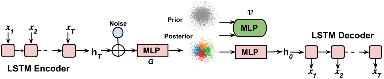
Figure 1: Illustration of the proposed implicit LVMs. $\nu(\boldsymbol{x},\boldsymbol{z})$ is used in iVAE, and $\nu(\boldsymbol{z})$ is used in iVAE${}_{\text{MI}}$. In this example, the piror is $p(\boldsymbol{z})=\mathcal{N}(0,1)$, the sample-based aggregated posterior $q(\boldsymbol{z})=\int q_{\boldsymbol{\phi}}(\boldsymbol{z}|\boldsymbol{x})q(\boldsymbol{x})d\boldsymbol{x}$ for four observations is shown, where the posterior $q_{\boldsymbol{\phi}}(\boldsymbol{z}|\boldsymbol{x})$ for each observation is visualized in a different color.

Dual form of KL-divergence

Though theoretically promising, the implicit representations in (6) render difficulties in optimizing the KL term $\mathcal{L}_{R}$ in (3), as the functional form is no longer tractable with implicit $q_{\boldsymbol{\phi}}(\boldsymbol{z}|\boldsymbol{x})$. We resort to evaluating its dual form based on Fenchel duality theorem Rockafellar et al. (1966); Dai et al. (2018):

$$\textsf{KL}\left(q_{\boldsymbol{\phi}}(\boldsymbol{z}|\boldsymbol{x})\parallel p(\boldsymbol{z})\right)$$ (7)

$$= \text{max}_{\nu}\mathbb{E}_{\boldsymbol{z}\sim q_{\boldsymbol{\phi}}(\boldsymbol{z}|\boldsymbol{x})}\nu_{\boldsymbol{\psi}}(\boldsymbol{x},\boldsymbol{z})-\mathbb{E}_{\boldsymbol{z}\sim p(\boldsymbol{z})}\text{exp}(\nu_{\boldsymbol{\psi}}(\boldsymbol{x},\boldsymbol{z})),$$

where $\nu_{\boldsymbol{\psi}}(\boldsymbol{x},\boldsymbol{z})$ is an auxiliary dual function, parameterized by a neural network with weights $\boldsymbol{\psi}$. By replacing the KL term with this dual form, the implicit VAE has the following objective:

$$\mathcal{L}_{\text{iVAE}} =\mathbb{E}_{\boldsymbol{x}\sim\mathcal{D}}\mathbb{E}_{\boldsymbol{z}\sim q_{\boldsymbol{\phi}}(\boldsymbol{z}|\boldsymbol{x})}\text{log}p_{\boldsymbol{\theta}}(\boldsymbol{x}|\boldsymbol{z})$$

$$-\mathbb{E}_{\boldsymbol{x}\sim\mathcal{D}}\mathbb{E}_{\boldsymbol{z}\sim q_{\boldsymbol{\phi}}(\boldsymbol{z}|\boldsymbol{x})}\nu_{\boldsymbol{\psi}}(\boldsymbol{x},\boldsymbol{z})$$

$$+\mathbb{E}_{\boldsymbol{x}\sim\mathcal{D}}\mathbb{E}_{\boldsymbol{z}\sim p(\boldsymbol{z})}\text{exp}(\nu_{\boldsymbol{\psi}}(\boldsymbol{x},\boldsymbol{z})),$$ (8)

Training scheme

Implicit VAE inherits the end-to-end training scheme of VAEs with extra work on training the auxiliary network $\nu_{\boldsymbol{\psi}}(\boldsymbol{x},\boldsymbol{z})$:

• Sample a mini-batch of $\boldsymbol{x}_{i}\sim\mathcal{D}$, $\epsilon_{i}\sim q(\epsilon)$, and generate $\boldsymbol{z}_{\boldsymbol{x}_{i},\epsilon_{i}}=G(\boldsymbol{x}_{i},\epsilon_{i};\boldsymbol{\phi})$; Sample a mini-batch of $\boldsymbol{z}_{i}\sim p(\boldsymbol{z})$.

• Update ${\boldsymbol{\psi}}$ in $\nu_{\boldsymbol{\psi}}(\boldsymbol{x},\boldsymbol{z})$ to maximize

  $$\sum_{i}\nu_{\boldsymbol{\psi}}(\boldsymbol{x}_{i},\boldsymbol{z}_{\boldsymbol{x}_{i},\epsilon_{i}})-\sum_{i}\text{exp}(\nu_{\boldsymbol{\psi}}(\boldsymbol{x}_{i},\boldsymbol{z}_{i}))$$ (9)

• Update parameters $\{\boldsymbol{\phi},\boldsymbol{\theta}\}$ to maximize

  $$\sum_{i}\text{log}p_{\boldsymbol{\theta}}(\boldsymbol{x}_{i}|\boldsymbol{z}_{\boldsymbol{x}_{i},\epsilon_{i}})-\sum_{i}\nu_{\boldsymbol{\psi}}(\boldsymbol{x}_{i},\boldsymbol{z}_{\boldsymbol{x}_{i},\epsilon_{i}})$$ (10)

In practice, we implement $\nu_{\boldsymbol{\psi}}(\boldsymbol{x},\boldsymbol{z})$ with a multilayer perceptron (MLP), which takes the concatenation of ${\boldsymbol{h}}$ and $\boldsymbol{z}$. In another word, the auxiliary network distinguishes between $(\boldsymbol{x},\boldsymbol{z}_{\boldsymbol{x}})$ and $(\boldsymbol{x},\boldsymbol{z})$, where $\boldsymbol{z}_{\boldsymbol{x}}$ is drawn from the posterior and $\boldsymbol{z}$ is drawn from the prior, respectively. We found the MLP-parameterized auxiliary network converges faster than LSTM encoder and decoder Hochreiter and Schmidhuber (1997). This means that the auxiliary network practically provides an accurate approximation to the KL regularization $\mathcal{L}_{R}$.

3.2 Mutual Information Regularized iVAE

It is noted the inherent deficiency of the original VAE objective in (3): the KL divergence regularization term matches each posterior distribution independently to the same prior. This is prone to posterior collapse in text generation, due to a strong auto-regressive decoder $p_{\boldsymbol{\theta}}(\boldsymbol{x}|\boldsymbol{z})$. When sequentially generating $x_{t}$, the model learns to solely rely on the ground-truth $[x_{1},\cdots,x_{t-1}]$, and ignore the dependency from $\boldsymbol{z}$ Fu et al. (2019). It results in the learned variational posteriors $q_{\boldsymbol{\phi}}(\boldsymbol{z}|\boldsymbol{x})$ to exactly match $p(\boldsymbol{z})$, without discriminating data $\boldsymbol{x}$.

To better regularize the latent space, we propose to replace $\mathcal{L}_{R}=\mathbb{E}_{\boldsymbol{x}\sim\mathcal{D}}\left[-\textsf{KL}\left(q_{\boldsymbol{\phi}}(\boldsymbol{z}|\boldsymbol{x})\parallel p(\boldsymbol{z})\right)\right]$ in (3), with the following KL divergence:

$$-\textsf{KL}\left(q_{\boldsymbol{\phi}}(\boldsymbol{z})\parallel p(\boldsymbol{z})\right),$$ (11)

where $q_{\boldsymbol{\phi}}(\boldsymbol{z})=\int q(\boldsymbol{x})q_{\boldsymbol{\phi}}(\boldsymbol{z}|\boldsymbol{x})d\boldsymbol{x}$ is the aggregated posterior, $q(\boldsymbol{x})$ is the empirical data distribution for the training dataset $\mathcal{D}$. The integral is estimated by ancestral sampling in practice, i.e. we first sample $\boldsymbol{x}$ from dataset and then sample $\boldsymbol{z}\sim q_{\boldsymbol{\phi}}(\boldsymbol{z}|\boldsymbol{x})$.

In (11), variational posterior is regularized as a whole $q_{\boldsymbol{\phi}}(\boldsymbol{z})$, encouraging posterior samples from different sentences to cooperate to satisfy the objective. It implies a solution that each sentence is represented as a local region in the latent space, the aggregated representation of all sentences match the prior; This avoids the degenerated solution from  (3) that the feature representation of individual sentence spans over the whole space.

Connection to mutual information

The proposed latent variable model coincides with Zhao et al. (2018, 2017a) where mutual information is introduced into the optimization, based on the following decomposition result (Please see detailed proof in Appendix A):

$$-\textsf{KL}\left(q_{\boldsymbol{\phi}}(\boldsymbol{z})\parallel p(\boldsymbol{z})\right) =I(\boldsymbol{x},\boldsymbol{z})$$

$$-\mathbb{E}_{\boldsymbol{x}}\textsf{KL}\left(q_{\boldsymbol{\phi}}(\boldsymbol{z}|\boldsymbol{x})\parallel p(\boldsymbol{z})\right),$$

where $I(\boldsymbol{x},\boldsymbol{z})$ is the mutual information between $\boldsymbol{z}$ and $\boldsymbol{x}$ under the joint distribution $q_{\boldsymbol{\phi}}(\boldsymbol{x},\boldsymbol{z})=q(\boldsymbol{x})q_{\boldsymbol{\phi}}(\boldsymbol{z}|\boldsymbol{x})$. Therefore, the objective in (11) also maximizes the mutual information between individual sentences and their latent features. We term the new LVM objective as iVAE${}_{\text{MI}}$:

$$\mathcal{L}_{\text{iVAE}_{\text{MI}}} =\mathbb{E}_{\boldsymbol{x}\sim\mathcal{D}}\mathbb{E}_{\boldsymbol{z}\sim q_{\boldsymbol{\phi}}(\boldsymbol{z}|\boldsymbol{x})}\text{log}p_{\boldsymbol{\theta}}(\boldsymbol{x}|\boldsymbol{z})$$

$$~{}~{}~{}~{}-\textsf{KL}\left(q_{\boldsymbol{\phi}}(\boldsymbol{z})\parallel p(\boldsymbol{z})\right)$$ (12)

Training scheme

Note that the aggregated posterior $q_{\boldsymbol{\phi}}(\boldsymbol{z})$ is also a sample-based distribution. Similarly, we evaluate (12) through its dual form:

$$\textsf{KL}\left(q_{\boldsymbol{\phi}}(\boldsymbol{z})\parallel p(\boldsymbol{z})\right)$$ (13)

$$= \text{max}_{\nu}\mathbb{E}_{\boldsymbol{z}\sim q_{\boldsymbol{\phi}}(\boldsymbol{z})}\nu_{\boldsymbol{\psi}}(\boldsymbol{z})-\mathbb{E}_{\boldsymbol{z}\sim p(\boldsymbol{z})}\text{exp}(\nu_{\boldsymbol{\psi}}(\boldsymbol{z})).$$

Therefore, iVAE${}_{\text{MI}}$ in (12) can be written as:

$$\mathcal{L}_{\text{iVAE}_{\text{MI}}} =\mathbb{E}_{\boldsymbol{x}\sim D}\mathbb{E}_{\boldsymbol{z}\sim q_{\boldsymbol{\phi}}(\boldsymbol{z}|\boldsymbol{x})}\text{log}p_{\boldsymbol{\theta}}(\boldsymbol{x}|\boldsymbol{z})$$ (14)

$$-\mathbb{E}_{\boldsymbol{z}\sim q_{\boldsymbol{\phi}}(\boldsymbol{z})}\nu_{\boldsymbol{\psi}}(\boldsymbol{z})+\mathbb{E}_{\boldsymbol{z}\sim p(\boldsymbol{z})}\text{exp}(\nu_{\boldsymbol{\psi}}(\boldsymbol{z})),$$

where the auxiliary network $\nu_{\boldsymbol{\psi}}(\boldsymbol{z})$ is parameterized as a neural network. Different from iVAE, $\nu_{\boldsymbol{\psi}}(\boldsymbol{z})$ in iVAE${}_{\text{MI}}$ only takes posterior samples as input. The training algorithm is similar to iVAE in Section 3.1, except a different auxiliary network $\nu_{\boldsymbol{\psi}}(\boldsymbol{z})$. In Appendix B, we show the full algorithm of iVAE${}_{\text{MI}}$.

We illustrate the proposed methods in Figure 1. Note that both iVAE and iVAE${}_{\text{MI}}$ share the same model architecture, except a different auxiliary network $\nu$.

4 Related Work

4.1 Solutions to posterior collapse

Several attempts have been made to alleviate the posterior collapse issue. The KL annealing scheme in language VAEs has been first used in  Bowman et al. (2015). An effective cyclical KL annealing schedule is used in Fu et al. (2019), where the KL annealing process is repeated multiple times. KL term weighting scheme is also adopted in $\beta$-VAE Higgins et al. (2017) for disentanglement. On model architecture side, dilated CNN was considered to replace auto-regressive LSTMs for decoding Yang et al. (2017). The bag-of-word auxiliary loss was proposed to improve the dependence on latent representations in generation Zhao et al. (2017b). More recently, lagging inference proposes to aggressively update encoder multiple times before a single decoder update He et al. (2019). Semi-amortized VAE refines variational parameters from an amortized encoder per instance with stochastic variational inference Kim et al. (2018).

All these efforts utilize the Gaussian-based forms for posterior inference. Our paper is among the first ones to attribute posterior collapse issue to the restrictive Gaussian assumption, and advocate more flexible sample-based representations.

4.2 Implicit Feature Learning

Sample-based distributions, as well as implicit features, have been widely used in representation learning Donahue et al. (2017); Li et al. (2017a). Vanilla autoencoders learn point masses of latent features rather than their distributions. Adversarial variational Bayes introduces an auxiliary discriminator network like GANs Goodfellow et al. (2014); Makhzani et al. (2015) to learn almost arbitrarily distributed latent variables Mescheder et al. (2017); Pu et al. (2017b). We explore the similar spirit in the natural language processing (NLP) domain. Amortized MCMC and particle based methods are introduced for LVM learning in Li et al. (2017d); Pu et al. (2017a); Chen et al. (2018). Coupled variational Bayes Dai et al. (2018) emphasizes an optimization embedding, i.e., a flow of particles, in a general setting of non-parametric variational inference. It also utilizes similar dual form with auxiliary function $\nu_{\boldsymbol{\psi}}(\boldsymbol{x},\boldsymbol{z})$ to evaluate KL divergence. Adversarially regularized autoencoders Makhzani et al. (2015); Kim et al. (2017) use similar objectives with iVAEs, in the form of a reconstruction error plus a specific regularization evaluated with implicit samples. Mutual information has also been considered into regularization in Zhao et al. (2018, 2017a) to obtain more informative representations.

Most previous works focus on image domain. It is largely unexplored in NLP. Further, the auto-regressive decoder renders an additional challenge when applying implicit latent representations. Adversarial training with samples can be empirically unstable, and slow even applying recent stabilization techniques in GANs Arjovsky et al. (2017); Gulrajani et al. (2017). To the best of our knowledge, this paper presents the first to effectively apply implicit feature representations, to NLP.

5 Experiments

In this section, the effectiveness of our methods is validated by largely producing supreme metrics on a broad range of text generation tasks under various scenarios. We note that when presenting our results in terms of perplexity and lower bounds, our evaluations are approximated. Thus they are not directly comparable to other methods. For a fair comparison, more advanced evaluation methods such as the annealing importance sampling should be adapted, which we leave as future work. Other evaluation metrics, e.g., the BLEU score, are fair to compare.

5.1 Language Modeling

Datasets.

We consider three public datasets, the Penn Treebank ($\mathtt{PTB}$) Marcus et al. (1993); Bowman et al. (2015), $\mathtt{Yahoo}$, and $\mathtt{Yelp}$ corpora Yang et al. (2017); He et al. (2019). $\mathtt{PTB}$ is a relatively small dataset with sentences of varying lengths, whereas $\mathtt{Yahoo}$ and $\mathtt{Yelp}$ contain larger amounts of long sentences. Detailed statistics of these datasets are shown in Table LABEL:table:lm_datasets.

Settings

We implement both encoder and decoder as one-layer LSTM. As illustrated in Figure 1, concatenation of the last hidden state of the encoder LSTM and a Gaussian noise is fed into a MLP to draw a posterior sample. When decoding, a latent sample is fed into a MLP to produce the initial hidden state of the decoder LSTM. A KL-term annealing scheme is also used Bowman et al. (2015). We list more detailed hyper-parameters and architectures in Appendix C.1.2.

Baselines.

We compare with several state-of-the-art VAE language modeling methods, including (1) VAEs with a monotonically KL-annealing schedule Bowman et al. (2015); (2) $\beta$-VAE Higgins et al. (2017), VAEs with a small penalty on KL term scaled by $\beta$; (3) SA-VAE Kim et al. (2018), mixing instance-specific variational inference with amortized inference; (4) Cyclical VAE Fu et al. (2019) that periodically anneals the KL term; (5) Lagging VAE, which aggressively updates encoder multiple times before a single decoder update.

Evaluation metrics.

Two categories of metrics are used to study VAEs for language modeling:

• To characterize the modeling ability of the observed sentences, we use the negative ELBO as the sum of reconstruction loss and KL term, as well as perplexity (PPL).

• Compared with traditional neural language models, VAEs has its unique advantages in feature learning. To measure the quality of learned features, we consider (1) KL: $\textsf{KL}\left(q_{\boldsymbol{\phi}}(\boldsymbol{z}|\boldsymbol{x})\parallel p(\boldsymbol{z})\right)$; (2) Mutual information (MI) $I(\boldsymbol{x},\boldsymbol{z})$ under the joint distribution $q_{\boldsymbol{\phi}}(\boldsymbol{x},\boldsymbol{z})$; (3) Number of active units (AU) of latent representation. The activity of a latent dimension $z$ is measured as $A_{\boldsymbol{z}}$$=\text{Cov}_{\boldsymbol{x}}\left(\mathbb{E}_{\boldsymbol{z}\sim q(\boldsymbol{z}|\boldsymbol{x})}\left[z\right]\right)$, which is defined as active if $A_{\boldsymbol{z}}$$>0.01$.

The evaluation of implicit LVMs is unexplored in language models, as there is no analytical forms for the KL term. We consider to evaluate both $\textsf{KL}\left(q_{\boldsymbol{\phi}}(\boldsymbol{z})\parallel p(\boldsymbol{z})\right)$ and $\textsf{KL}\left(q_{\boldsymbol{\phi}}(\boldsymbol{z}|\boldsymbol{x})\parallel p(\boldsymbol{z})\right)$ by training a fully connected $\nu$ network following Eq. (7) and (13). To avoid the inconsistency between $\nu(\boldsymbol{x},\boldsymbol{z})$ and $\nu(\boldsymbol{z})$ networks due to training, we train them using the same data and optimizer in every iteration. We evaluate each distribution $q_{\boldsymbol{\phi}}(\boldsymbol{z}|\boldsymbol{x})$ with 128 latent samples per $\boldsymbol{x}$. We report the KL terms until their learning curves are empirically converged. Note that our evaluation is different from exact PPL in two ways: (1) It is a bound of $\log p(\boldsymbol{x})$ (similar to all text VAE model in the literature); (2) the KL term in the bound is estimated using samples, rather than a closed form.

We report the results in Table LABEL:table:languagemodeling. A better language model would pursue a lower negative ELBO (also lower reconstruction errors, lower PPL), and make sufficient use of the latent space (i.e., maintain relatively high KL term, higher mutual information and more active units). Under all these metrics, the proposed iVAEs achieve much better performance. The posterior collapse issue is largely alleviated as indicated by the improved KL and MI values, especially with iVAE${}_{\text{MI}}$ which directly takes mutual information into account.

The comparison on training time is shown in Table LABEL:table:lm_traintime. iVAE and iVAE${}_{\text{MI}}$ requires updating an auxiliary network, it spends $30\%$ more time than traditional VAEs. This is more efficient than SA-VAE and Lag-VAE.

Table 4: Interpolating latent representation.

Latent space interpolation.

One favorable property of VAEs Bowman et al. (2015); Zhao et al. (2018) is to provide smooth latent representations that capture sentence semantics. We demonstrate this by interpolating two latent feature, each of which represents a unique sentence. Table 4 shows the generated examples. We take two sentences $\boldsymbol{x}_{1}$ and $\boldsymbol{x}_{2}$, and obtain their latent features as the sample-averaging results for $\boldsymbol{z}_{1}$ and $\boldsymbol{z}_{2}$, respectively, from the implicit encoder, and then greedily decode conditioned on the interpolated feature $\boldsymbol{z}_{t}=\boldsymbol{z}_{1}\cdot(1-t)+\boldsymbol{z}_{2}\cdot t$ with $t$ increased from 0 to 1 by a step size of 0.1. It generates sentences with smooth semantic evolution.

Improved Decoder.

One might wonder whether the improvements come from simply having a more flexible encoder during evaluation, rather than from utilizing high-quality latent features, and learning a better decoder. We use $\mathtt{PTB}$ to confirm our findings. We draw samples from the prior $p(\boldsymbol{z})$, and greedily decode them using the trained decoder. The quality of the generated text is evaluated by an external library “KenLM Language Model Toolkit” Heafield et al. (2013) with two metrics Kim et al. (2017): (1) Forward PPL: the fluency of the generated text based on language models derived from the $\mathtt{PTB}$ training corpus; (2) Reverse PPL: the fluency of $\mathtt{PTB}$ corpus based on language model derived from the generated text, which measures the extent to which the generations are representative of the $\mathtt{PTB}$ underlying language model. For both the PPL numbers, the lower the better. We use n=5 for n-gram language models in “KenLM”.

As shown in Table LABEL:table:forward_reverse, implicit LVMs outperform others in both PPLs, which confirms that the implicit representation can lead to better decoders. The vanilla VAE model performs the worst. This is expected, as the posterior collapse issue results in poor utilization of a latent space. Besides, we can see that iVAE${}_{\text{MI}}$ generates comparably fluent but more diverse text than pure iVAE, from the lower reverse PPL values. This is reasonable, due to the ability of iVAE${}_{\text{MI}}$ to encourage diverse latent samples per sentence with the aggregated regularization in the latent space.

5.2 Unaligned style transfer

We next consider the task of unaligned style transfer, which represents a scenario to generate text with desired specifications. The goal is to control one style aspect of a sentence that is independent of its content. We consider non-parallel corpora of sentences, where the sentences in two corpora have the same content distribution but with different styles, and no paired sentence is provided.

Model Extension.

The success of this task depends on the exploitation of the distributional equivalence of content to learn sentiment independent content code and decoding it to a different style. To ensure such independence, we extend iVAE${}_{\text{MI}}$ by adding a sentiment classifier loss to its objective (14), similar to the previous style transfer methods Shen et al. (2017); Kim et al. (2017). Let $y$ be the style attribute, $\boldsymbol{x}_{p}$ and $\boldsymbol{x}_{n}$ (with corresponding features $\boldsymbol{z}_{p}$, $\boldsymbol{z}_{n}$) be sentences with positive and negative sentiments , respectively. The style classifier loss $\mathcal{L}_{\text{class}}(\boldsymbol{z}_{p},\boldsymbol{z}_{n})$ is the cross entropy loss of a binary classifier.

The classifier and encoder are trained adversarially: (1) the classifier is trained to distinguish latent features with different sentiments; (2) the encoder is trained to fool the classifier in order to remove distinctions of content features from sentiments. In practice, the classifier is implemented as a MLP. We implement two separate decoder LSTMs for clean sentiment decoding: one for positive $p(\boldsymbol{x}|\boldsymbol{z},y=1)$, and one for negative sentiment $p(\boldsymbol{x}|\boldsymbol{z},y=0)$. The prior $p(\boldsymbol{z})$ is also implemented as an implicit distribution, via transforming noise from a standard Gaussian through a MLP. Appendix C.2.2 lists more details.

Baseline.

We compare iVAE${}_{\text{MI}}$ with a state-of-the-art unaligned sentiment transferer: the adversarially regularized autoencoder (ARAE) Kim et al. (2017), which directly regularizes the latent space with Wasserstein distance measure.

Table 6: Sentiment transfer on $\mathtt{Yelp}$. (Up: From negative to positive, Down: From positive to negative.)

Datasets.

Following Shen et al. (2017), the $\mathtt{Yelp}$ restaurant reviews dataset is processed from the original $\mathtt{Yelp}$ dataset in language modeling. Reviews with user rating above three are considered positive, and those below three are considered negative. The pre-processing allows sentiment analysis on sentence level with feasible sentiment, ending up with shorter sentences with each at most 15 words than those in language modeling. Finally, we get two sets of unaligned reviews: 250K negative sentences, and 350K positive ones. Other dataset details are shown in Appendix C.2.1.

Evaluation Metrics.

(1) Acc: the accuracy of transferring sentences into another sentiment measured by an automatic classifier: the “fasttext” library Joulin et al. (2017); (2) BLEU: the consistency between the transferred text and the original; (3) PPL: the reconstruction perplexity of original sentences without altering sentiment; (4) RPPL: the reverse perplexity that evaluates the training corpus based on language model derived from the generated text, which measures the extent to which the generations are representative of the training corpus; (5) Flu: human evaluated index on the fluency of transferred sentences when read alone (1-5, 5 being most fluent as natural language); (6) Sim: the human evaluated similarity between the original and the transferred sentences in terms of their contents (1-5, 5 being most similar). Note that the similarity measure doesn’t care sentiment but only the topic covered by sentences. For human evaluation, we show 1000 randomly selected pairs of original and transferred sentences to crowdsourcing readers, and ask them to evaluate the ”Flu” and ”Sim” metrics stated above. Each measure is averaged among crowdsourcing readers.

As shown in Table LABEL:table:sentiment, iVAE${}_{\text{MI}}$ outperforms ARAE in metrics except Acc, showing that iVAE${}_{\text{MI}}$ captures informative representations, generates consistently opposite sentences with similar grammatical structure and reserved semantic meaning. Both methods perform successful sentiment transfer as shown by Acc values. iVAE${}_{\text{MI}}$ achieves a little lower Acc due to much more content reserving, even word reserving, of the source sentences.

Table 6 presents some examples. In each box, we show the source sentence, the transferred sentence by ARAE and iVAE${}_{\text{MI}}$, respectively. We observe that ARAE usually generates new sentences that miss the content of the source, while iVAE${}_{\text{MI}}$ shows better content-preserving.

5.3 Dialog response generation

We consider the open-domain dialog response generation task, where we need to generate a natural language response given a dialog history. It is crucial to learn a meaningful latent feature representation of the dialog history in order to generate a consistent, relevant, and contentful response that is likely to drive the conversation Gao et al. (2019).

Datasets.

We consider two mainstream datasets in recent studies Zhao et al. (2017b, 2018); Fu et al. (2019); Gu et al. (2018): $\mathtt{Switchboard}$ Godfrey and Holliman (1997) and $\mathtt{Dailydialog}$ Li et al. (2017c). $\mathtt{Switchboard}$ contains 2,400 two-way telephone conversations under 70 specified topics. $\mathtt{Dailydialog}$ has 13,118 daily conversations for a English learner. We process each utterance as the response of previous 10 context utterances from both speakers. The datasets are separated into training, validation, and test sets as convention: 2316:60:62 for $\mathtt{Switchboard}$ and 10:1:1 for $\mathtt{Dailydialog}$, respectively.

Model Extension.

We adapt iVAE${}_{\text{MI}}$ by integrating the context embedding $\boldsymbol{c}$ into all model components. The prior $p(\boldsymbol{z}|\boldsymbol{c})$ is defined as an implicit mapping between context embedding $\boldsymbol{c}$ and prior samples, which is not pre-fixed but learned together with the variational posterior for more modeling flexibility. The encoder $q(\boldsymbol{z}|\boldsymbol{x},\boldsymbol{c})$, auxiliary dual function $\nu_{\boldsymbol{\psi}}(\boldsymbol{z},\boldsymbol{c})$ and decoder $p(\boldsymbol{x}|\boldsymbol{c},\boldsymbol{z})$ depend on context embedding $\boldsymbol{c}$ as well. Both encoder and decoder are implemented as GRUs. The utterance encoder is a bidirectional GRU with 300 hidden units in each direction. The context encoder and decoder are both GRUs with 300 hidden units. Appendix C.3.1 presents more training details.

Baseline.

We benchmark representative baselines and state-of-the-art approaches, include: SeqGAN, a GAN based model for sequence generation Li et al. (2017b); CVAE baseline Zhao et al. (2017b); dialogue WAE, a conditional Wasserstein auto-encoder for response generation Gu et al. (2018).

Evaluation Metrics.

We adopt several widely used numerical metrics to systematically evaluate the response generation, including BLEU score Papineni et al. (2002), BOW Embedding Liu et al. (2016) and Distinct Li et al. (2015), as used in Gu et al. (2018). For each testing context, we sample 10 responses from each model.

• BLEU measures how much a generated response contains n-gram overlaps with the references. We compute 4-gram BLEU. For each test context, we sample 10 responses from the models and compute their BLEU scores. BLEU precision and recall is defind as the average and maximum scores, respectively Zhao et al. (2017b).

• BOW embedding is the cosine similarity of bag-of-words embeddings between the generations and the reference. We compute three different BOW embedding: greedy, average, and extreme.

• Distinct evaluates the diversity of the generated responses: dist-n is defined as the ratio of unique n-grams (n=1,2) over all n-grams in the generated responses. We evaluate diversities for both within each sampled response and among all responses as intra-dist and inter-dist, respectively.

Tables LABEL:table:dialogue show the performance comparison. iVAE${}_{\text{MI}}$ achieves consistent improvement on a majority of the metrics. Especially, the BOW embeddings and Distinct get significantly improvement, which implies that iVAE${}_{\text{MI}}$ produces both meaningful and diverse latent representations.

6 Conclusion

We present two types of implicit deep latent variable models, iVAE and iVAE${}_{\text{MI}}$. Core to these two models is the sample-based representation of the latent features in LVM, in replacement of traditional Gaussian-based distributions. Extensive experiments show that the proposed implicit LVM models consistently outperform the vanilla VAEs on three tasks, including language modeling, style transfer and dialog response generation.

Acknowledgments

We acknowledge Yufan Zhou for helpful discussions and the reviewers for their comments. The authors appreciate some peer researchers for discussing with us the approximation nature of our metrics, such as perplexity and KL terms, among whom are Leo Long and Liqun Chen.

Appendix

Appendix A Decomposition of the regularization term

We have the following decomposition

$$-\textsf{KL}\left(q_{\boldsymbol{\phi}}(\boldsymbol{z})\parallel p(\boldsymbol{z})\right)$$

$$=-\mathbb{E}_{\boldsymbol{z}\sim q_{\boldsymbol{\phi}}(\boldsymbol{z})}\left[\text{log}q_{\boldsymbol{\phi}}(\boldsymbol{z})-\text{log}p(\boldsymbol{z})\right]$$

$$=H\left(q_{\boldsymbol{\phi}}(\boldsymbol{z})\right)+\mathbb{E}_{\boldsymbol{z}\sim q_{\boldsymbol{\phi}}(\boldsymbol{z})}\text{log}p(\boldsymbol{z})$$

$$=H\left(q_{\boldsymbol{\phi}}(\boldsymbol{z})\right)+\mathbb{E}_{\boldsymbol{x}}\mathbb{E}_{\boldsymbol{z}\sim q_{\boldsymbol{\phi}}(\boldsymbol{z}|\boldsymbol{x})}\text{log}q_{\boldsymbol{\phi}}(\boldsymbol{z}|\boldsymbol{x})$$

$$-\mathbb{E}_{\boldsymbol{x}}\mathbb{E}_{\boldsymbol{z}\sim q_{\boldsymbol{\phi}}(\boldsymbol{z}|\boldsymbol{x})}\text{log}q_{\boldsymbol{\phi}}(\boldsymbol{z}|\boldsymbol{x})+\mathbb{E}_{\boldsymbol{z}\sim q_{\boldsymbol{\phi}}(\boldsymbol{z})}\text{log}p(\boldsymbol{z})$$

$$=H\left(q_{\boldsymbol{\phi}}(\boldsymbol{z})\right)-H\left(q_{\boldsymbol{\phi}}(\boldsymbol{z}|\boldsymbol{x})\right)$$

$$-\mathbb{E}_{\boldsymbol{x}}\mathbb{E}_{\boldsymbol{z}\sim q_{\boldsymbol{\phi}}(\boldsymbol{z}|\boldsymbol{x})}\text{log}q_{\boldsymbol{\phi}}(\boldsymbol{z}|\boldsymbol{x})+\mathbb{E}_{\boldsymbol{z}\sim q_{\boldsymbol{\phi}}(\boldsymbol{z})}\text{log}p(\boldsymbol{z})$$

$$=I(\boldsymbol{x},\boldsymbol{z})-\mathbb{E}_{\boldsymbol{x}}\mathbb{E}_{\boldsymbol{z}\sim q_{\boldsymbol{\phi}}(\boldsymbol{z}|\boldsymbol{x})}\text{log}q_{\boldsymbol{\phi}}(\boldsymbol{z}|\boldsymbol{x})$$

$$+\mathbb{E}_{\boldsymbol{x}}\mathbb{E}_{\boldsymbol{z}\sim q_{\boldsymbol{\phi}}(\boldsymbol{z}|\boldsymbol{x})}\text{log}p(\boldsymbol{z})$$

$$=I(\boldsymbol{x},\boldsymbol{z})-\mathbb{E}_{\boldsymbol{x}}\textsf{KL}\left(q_{\boldsymbol{\phi}}(\boldsymbol{z}|\boldsymbol{x})\parallel p(\boldsymbol{z})\right)$$

where $q_{\boldsymbol{\phi}}(\boldsymbol{z})=\int q(\boldsymbol{x})q_{\boldsymbol{\phi}}(\boldsymbol{z}|\boldsymbol{x})dx$$=\mathbb{E}_{\boldsymbol{x}}\left[q_{\boldsymbol{\phi}}(\boldsymbol{z}|\boldsymbol{x})\right]$, $q(\boldsymbol{x})$ is the empirical data distribution for the training dataset $\mathcal{D}$; $H(\cdot)$ is the Shannon entropy and $I(\boldsymbol{x},\boldsymbol{z})=H(\boldsymbol{z})-H(\boldsymbol{z}|\boldsymbol{x})$ is the mutual information between $z$ and $x$ under the joint distribution $q_{\boldsymbol{\phi}}(\boldsymbol{x},\boldsymbol{z})=q(\boldsymbol{x})q_{\boldsymbol{\phi}}(\boldsymbol{z}|\boldsymbol{x})$.

Appendix B Training scheme of iVAE${}_{\text{MI}}$

The full training scheme of iVAE${}_{\text{MI}}$ is as following after substituting the auxiliary network of implicit VAE:

• Sample mini batch $\boldsymbol{x}_{i}\sim\mathcal{D}$, $\epsilon_{i}\sim q(\epsilon)$, $\boldsymbol{z}_{i}\sim p(\boldsymbol{z})$ and generate $\boldsymbol{z}_{\boldsymbol{x}_{i},\epsilon_{i}}=G(\boldsymbol{x}_{i},\epsilon_{i};\boldsymbol{\phi})$;

• Update $\nu_{\boldsymbol{\psi}}(\boldsymbol{z})$ net to maximize $\sum_{i}\nu_{\boldsymbol{\psi}}(\boldsymbol{z}_{\boldsymbol{x}_{i},\epsilon_{i}})$-$\sum_{i}\text{exp}(\nu_{\boldsymbol{\psi}}(\boldsymbol{z}_{i}))$ according to Eq. (14);

• Update parameters $\boldsymbol{\phi}$, $\boldsymbol{\theta}$ to maximize $\sum_{i}\text{log}p_{\boldsymbol{\theta}}(\boldsymbol{x}_{i}|\boldsymbol{z}_{\boldsymbol{x}_{i},\epsilon_{i}})$-$\sum_{i}\nu_{\boldsymbol{\psi}}(\boldsymbol{z}_{\boldsymbol{x}_{i},\epsilon_{i}})$ according to Eq. (14).

Appendix C Experimental details

C.1 Language modeling

C.1.1 Data details

The details of the three datasets are shown below. Each datasets contain “train”, “validate” and “test” text files with each sentence in one line.

C.1.2 More training details

We basically follow the architecture specifications in Kim et al. (2018). They have an encoder predicting posterior mean and variance and we have an implicit encoder which predicts code samples directly from LSTM encoding and Gaussian noise.

We implement both encoder and decoder as one-layer LSTMs with 1024 hidden units and 512-dimensional word embeddings (in $\mathtt{PTB}$, these numbers are 512 and 256). The $\nu$ network is a fully connected network whose hidden units are 512-512-512-1. The vocabulary size is 20K for $\mathtt{Yahoo}$ and $\mathtt{Yelp}$ and 10K for $\mathtt{PTB}$. The last hidden state of the encoder concatenated with a 32-dimensional Gaussian noise is used to sample 32-dimensional latent codes, which is then adopted to predict the initial hidden state of the decoder LSTM and additionally fed as input to each step at the LSTM decoder. A KL-cost annealing strategy is commonly used Bowman et al. (2015), where the scalar weight on the KL term is increased linearly from 0.1 to 1.0 each batch over 10 epochs. There are dropout layers with probability 0.5 between the input-to-hidden layer and the hidden-to-output layer on the decoder LSTM only.

All models are trained with Adam optimizer, when encoder and decoder LSTM use learning rate 1e-3 or 8e-4, and $\nu$ network uses learning rate 1e-5 and usually update 5 times versus a single LSTM end-to-end update. We train for 30$\sim$40 epochs, which is enough for convergence for all models. Model parameters are initialized over $U(-0.01,0.01)$ and gradients are clipped at 5.0.

SA-VAE runs with 10 refinement steps.

C.2 Unsupervised style transfer

C.2.1 Processing details

The pre-processing allows sentiment analysis on sentence level with feasible sentiment, ending up with shorter sentences with each at most 15 words than those in language modeling. Finally, we get two sets of unaligned reviews: 250K negative sentences, and 350K positive ones. They are then divided in ratio 7:1:2 to train, validate, and test data.

C.2.2 More training details

The vocabulary size is 10K after replacing words occurring less than 5 times with the “$<$unk$>$” token. The encoder and decoder are all an one-layer LSTM with 128 hidden units. The word embedding size is 128 with latent content code dimension 32. When LSTMs are trained with SGD optimizer with 1.0 learning rate, other fully connected neural nets are all trained with Adam optimizer with initial learning rate 1e-4. A grad clipping on the LSTMs is performed before each update, with max grad norm set to 1. The prior net, $\nu$ auxiliary net, and style classifier are all implemented with 2 hidden layer (not include output layer) with 128-128 hidden units. The $\nu$ network is trained 5 iterations versus other networks with single iteration with each mini-batch for performing accurate regularization. The “fasttext” python library Joulin et al. (2017) is needed to evaluate accuracy, and “KenLM Language Model Toolkit” Heafield et al. (2013) is needed to evaluate reverse PPL.

C.3 Dialog response generation

C.3.1 More training details

Both encoder and decoder are implemented as GRUs. The utterance encoder is a bidirectional GRU with 300 hidden units in each direction. The context encoder and decoder are both GRUs with 300 hidden units. The prior and the recognition networks (implicit mappings) are both 2-layer feed-forward networks of size 200 with tanh non-linearity to sample Gaussian noise plus 3-layer feed-forward networks to implicitly generate samples with ReLU non-linearity and hidden sizes of 200, 200 and 400, respectively. The dimension of a latent variable z is set to 200. The initial weights for all fully connected layers are sampled from a uniform distribution [-0.02, 0.02]. We set the vocabulary size to 10,000 and define all the out-of-vocabulary words to a special token “$<$unk$>$”. The word embedding size is 200 and initialized with pre-trained Glove vectors Pennington et al. (2014) on Twitter. The size of context window is set to 10 with a maximum utterance length of 40. We sample responses with greedy decoding so that the randomness entirely come from the latent variables. The GRUs are trained by SGD optimizer with an initial learning rate of 1.0, decay rate 0.4 and gradient clipping at 1. The fully connected neural nets are trained by RMSprop optimizer with fixed learning rates of 5e-5, except the $\nu$ net is trained with learning rate 1e-5 and repeatedly 5 inner iterations.

References

- Arjovsky et al. (2017) Martín Arjovsky, Soumith Chintala, and Léon Bottou. 2017. Wasserstein gan. CoRR, abs/1701.07875.
- Bowman et al. (2015) Samuel R Bowman, Luke Vilnis, Oriol Vinyals, Andrew M Dai, Rafal Jozefowicz, and Samy Bengio. 2015. Generating sentences from a continuous space. arXiv preprint arXiv:1511.06349.
- Chen et al. (2018) Changyou Chen, Chunyuan Li, Liqun Chen, Wenlin Wang, Yunchen Pu, and Lawrence Carin. 2018. Continuous-time flows for efficient inference and density estimation. ICML.
- Cremer et al. (2018) Chris Cremer, Xuechen Li, and David Duvenaud. 2018. Inference suboptimality in variational autoencoders. arXiv preprint arXiv:1801.03558.
- Dai et al. (2018) Bo Dai, Hanjun Dai, Niao He, Weiyang Liu, Zhen Liu, Jianshu Chen, Lin Xiao, and Le Song. 2018. Coupled variational bayes via optimization embedding. In S. Bengio, H. Wallach, H. Larochelle, K. Grauman, N. Cesa-Bianchi, and R. Garnett, editors, Advances in Neural Information Processing Systems 31, pages 9713–9723. Curran Associates, Inc.
- Donahue et al. (2017) Jeff Donahue, Philipp Krähenbühl, and Trevor Darrell. 2017. Adversarial feature learning. ICLR.
- Fu et al. (2019) Hao Fu, Chunyuan Li, Xiaodong Liu, Jianfeng Gao, Asli Celikyilmaz, and Lawrence Carin. 2019. Cyclical annealing schedule: A simple approach to mitigating kl vanishing. NAACL.
- Gao et al. (2019) Jianfeng Gao, Michel Galley, and Lihong Li. 2019. Neural approaches to conversational ai. Foundations and Trends® in Information Retrieval, 13(2-3):127–298.
- Godfrey and Holliman (1997) John J Godfrey and Edward Holliman. 1997. Switchboard-1 release 2. Linguistic Data Consortium, Philadelphia, 926:927.
- Goodfellow et al. (2014) Ian Goodfellow, Jean Pouget-Abadie, Mehdi Mirza, Bing Xu, David Warde-Farley, Sherjil Ozair, Aaron Courville, and Yoshua Bengio. 2014. Generative adversarial nets. In Z. Ghahramani, M. Welling, C. Cortes, N. D. Lawrence, and K. Q. Weinberger, editors, Advances in Neural Information Processing Systems 27, pages 2672–2680. Curran Associates, Inc.
- Gu et al. (2018) Xiaodong Gu, Kyunghyun Cho, Jungwoo Ha, and Sunghun Kim. 2018. Dialogwae: Multimodal response generation with conditional wasserstein auto-encoder. arXiv preprint arXiv:1805.12352.
- Gulrajani et al. (2017) Ishaan Gulrajani, Faruk Ahmed, Martin Arjovsky, Vincent Dumoulin, and Aaron Courville. 2017. Improved training of wasserstein gans. In Advances in Neural Information Processing Systems 30, pages 5769–5779. Arxiv: 1704.00028.
- He et al. (2019) Junxian He, Daniel Spokoyny, Graham Neubig, and Taylor Berg-Kirkpatrick. 2019. Lagging inference networks and posterior collapse in variational autoencoders. arXiv preprint arXiv:1901.05534.
- Heafield et al. (2013) Kenneth Heafield, Ivan Pouzyrevsky, Jonathan H. Clark, and Philipp Koehn. 2013. Scalable modified Kneser-Ney language model estimation. In Proceedings of the 51st Annual Meeting of the Association for Computational Linguistics, pages 690–696, Sofia, Bulgaria.
- Higgins et al. (2017) Irina Higgins, Loic Matthey, Arka Pal, Christopher Burgess, Xavier Glorot, Matthew Botvinick, Shakir Mohamed, and Alexander Lerchner. 2017. beta-vae: Learning basic visual concepts with a constrained variational framework. In International Conference on Learning Representations, volume 3.
- Hochreiter and Schmidhuber (1997) Sepp Hochreiter and Jürgen Schmidhuber. 1997. Long short-term memory. Neural computation, 9(8):1735–1780.
- Hu et al. (2017) Zhiting Hu, Zichao Yang, Xiaodan Liang, Ruslan Salakhutdinov, and Eric P Xing. 2017. Toward controlled generation of text. In Proceedings of the 34th International Conference on Machine Learning-Volume 70, pages 1587–1596. JMLR. org.
- Joulin et al. (2017) Armand Joulin, Edouard Grave, Piotr Bojanowski, and Tomas Mikolov. 2017. Bag of tricks for efficient text classification. In Proceedings of the 15th Conference of the European Chapter of the Association for Computational Linguistics: Volume 2, Short Papers, pages 427–431. Association for Computational Linguistics.
- Kim et al. (2018) Yoon Kim, Sam Wiseman, Andrew Miller, David Sontag, and Alexander Rush. 2018. Semi-amortized variational autoencoders. In International Conference on Machine Learning, pages 2683–2692.
- Kim et al. (2017) Yoon Kim, Kelly Zhang, Alexander M Rush, Yann LeCun, et al. 2017. Adversarially regularized autoencoders. arXiv preprint arXiv:1706.04223.
- Kingma and Welling (2013) Diederik P Kingma and Max Welling. 2013. Auto-encoding variational bayes. arXiv preprint arXiv:1312.6114.
- Li et al. (2017a) Chunyuan Li, Hao Liu, Changyou Chen, Yuchen Pu, Liqun Chen, Ricardo Henao, and Lawrence Carin. 2017a. Alice: Towards understanding adversarial learning for joint distribution matching. In Advances in Neural Information Processing Systems, pages 5495–5503.
- Li et al. (2015) Jiwei Li, Michel Galley, Chris Brockett, Jianfeng Gao, and Bill Dolan. 2015. A diversity-promoting objective function for neural conversation models. arXiv preprint arXiv:1510.03055.
- Li et al. (2017b) Jiwei Li, Will Monroe, Tianlin Shi, Sébastien Jean, Alan Ritter, and Dan Jurafsky. 2017b. Adversarial learning for neural dialogue generation. arXiv preprint arXiv:1701.06547.
- Li et al. (2017c) Yanran Li, Hui Su, Xiaoyu Shen, Wenjie Li, Ziqiang Cao, and Shuzi Niu. 2017c. Dailydialog: A manually labelled multi-turn dialogue dataset. arXiv preprint arXiv:1710.03957.
- Li et al. (2017d) Yingzhen Li, Richard E Turner, and Qiang Liu. 2017d. Approximate inference with amortised mcmc. arXiv preprint arXiv:1702.08343.
- Liu et al. (2016) Chia-Wei Liu, Ryan Lowe, Iulian V Serban, Michael Noseworthy, Laurent Charlin, and Joelle Pineau. 2016. How not to evaluate your dialogue system: An empirical study of unsupervised evaluation metrics for dialogue response generation. arXiv preprint arXiv:1603.08023.
- Makhzani et al. (2015) Alireza Makhzani, Jonathon Shlens, Navdeep Jaitly, Ian Goodfellow, and Brendan Frey. 2015. Adversarial autoencoders. arXiv preprint arXiv:1511.05644.
- Marcus et al. (1993) Mitchell Marcus, Beatrice Santorini, and Mary Ann Marcinkiewicz. 1993. Building a large annotated corpus of english: The penn treebank. Computational Linguistics.
- Mescheder et al. (2017) Lars Mescheder, Sebastian Nowozin, and Andreas Geiger. 2017. Adversarial variational bayes: Unifying variational autoencoders and generative adversarial networks. In Proceedings of the 34th International Conference on Machine Learning-Volume 70, pages 2391–2400. JMLR. org.
- Miao et al. (2016) Yishu Miao, Lei Yu, and Phil Blunsom. 2016. Neural variational inference for text processing. In International conference on machine learning, pages 1727–1736.
- Papineni et al. (2002) Kishore Papineni, Salim Roukos, Todd Ward, and Wei-Jing Zhu. 2002. Bleu: a method for automatic evaluation of machine translation. In Proceedings of the 40th annual meeting on association for computational linguistics, pages 311–318. Association for Computational Linguistics.
- Pennington et al. (2014) Jeffrey Pennington, Richard Socher, and Christopher Manning. 2014. Glove: Global vectors for word representation. In Proceedings of the 2014 conference on empirical methods in natural language processing (EMNLP), pages 1532–1543.
- Pu et al. (2017a) Yuchen Pu, Zhe Gan, Ricardo Henao, Chunyuan Li, Shaobo Han, and Lawrence Carin. 2017a. Vae learning via stein variational gradient descent. In Advances in Neural Information Processing Systems, pages 4236–4245.
- Pu et al. (2017b) Yuchen Pu, Weiyao Wang, Ricardo Henao, Liqun Chen, Zhe Gan, Chunyuan Li, and Lawrence Carin. 2017b. Adversarial symmetric variational autoencoder. In Advances in Neural Information Processing Systems, pages 4330–4339.
- Rezende et al. (2014) Danilo Jimenez Rezende, Shakir Mohamed, and Daan Wierstra. 2014. Stochastic backpropagation and approximate inference in deep generative models. In International Conference on Machine Learning, pages 1278–1286.
- Rockafellar et al. (1966) R Tyrrell Rockafellar et al. 1966. Extension of fenchel’duality theorem for convex functions. Duke mathematical journal, 33(1):81–89.
- Shah and Barber (2018) Harshil Shah and David Barber. 2018. Generative neural machine translation. In S. Bengio, H. Wallach, H. Larochelle, K. Grauman, N. Cesa-Bianchi, and R. Garnett, editors, Advances in Neural Information Processing Systems 31, pages 1346–1355. Curran Associates, Inc.
- Shen et al. (2017) Tianxiao Shen, Tao Lei, Regina Barzilay, and Tommi Jaakkola. 2017. Style transfer from non-parallel text by cross-alignment. In Advances in neural information processing systems, pages 6830–6841.
- Yang et al. (2017) Zichao Yang, Zhiting Hu, Ruslan Salakhutdinov, and Taylor Berg-Kirkpatrick. 2017. Improved variational autoencoders for text modeling using dilated convolutions. In Proceedings of the 34th International Conference on Machine Learning-Volume 70, pages 3881–3890. JMLR. org.
- Zhao et al. (2017a) Shengjia Zhao, Jiaming Song, and Stefano Ermon. 2017a. InfoVAE: Information maximizing variational autoencoders. arXiv preprint arXiv:1706.02262.
- Zhao et al. (2018) Tiancheng Zhao, Kyusong Lee, and Maxine Eskenazi. 2018. Unsupervised discrete sentence representation learning for interpretable neural dialog generation. arXiv preprint arXiv:1804.08069.
- Zhao et al. (2017b) Tiancheng Zhao, Ran Zhao, and Maxine Eskenazi. 2017b. Learning discourse-level diversity for neural dialog models using conditional variational autoencoders. arXiv preprint arXiv:1703.10960.