The spectrum of the light component of TeV cosmic rays measured with HAWC

Abstract:

We present a measurement of the energy spectrum of the light mass group of cosmic rays (protons and helium) with the High Altitude Water Cherenkov (HAWC) Observatory in the energy interval from $10$ TeV to $200$ TeV. The spectrum covers the energy range between direct and indirect measurements, where precision data on the composition of cosmic rays are needed. The spectrum was constructed by applying an unfolding technique on a proton plus helium enriched sub-sample ($>90\%$ abundance) of cosmic ray air showers selected from the HAWC cosmic-ray data. The subset contains $3.8\times 10^{9}$ air shower events with primary energies in the interval $1$ TeV to $300$ TeV and zenith angles less than $16.7$ degrees. Mass selection was performed using an analysis of the lateral age parameter of air shower events, based on both CORSIKA/QGSJET-II-03 simulations and event-by-event measurements on the lateral structure of the shower front and the primary energy of the showers.

1 Introduction

The energy region from $10^{13}\,\mbox{eV}$ to $10^{15}\,\mbox{eV}$ of the cosmic ray energy spectrum has been barely explored as it is located at the frontier between the direct and indirect detection techniques. However, it is of great interest due to the possible presence of new structures in the spectra of all-particles and elemental mass groups of cosmic rays in this energy regime (see, for example, [1, 2, 5, 4]). To investigate the possible existence of such structures, TeV cosmic-ray data with good precision and high statistics are required and HAWC can contribute to this task due to its capabilities. HAWC is an extensive air shower (EAS) observatory located at $4,100\,\mbox{m}$ a.s.l. ($\sim 640\,\mbox{g}/\mbox{cm}^{2}$ atmospheric depth) on the northern slope of the volcano Sierra Negra in Mexico. The instrument is designed to detect $\gamma$ rays from $100\,\mbox{GeV}$ to $100\,\mbox{TeV}$, but its altitude and physical dimensions permit measurements of primary hadronic cosmic rays up to PeV energies. In this contribution, we will present a description of an unfolding analysis to estimate the proton plus helium spectrum of cosmic rays in the energy interval $10$ TeV to $200$ TeV with HAWC. We will also show the result and we will compare it with the measurements of other direct and indirect experiments.

2 Event reconstruction and simulation

HAWC is composed of $300$ water Cherenkov detectors (WCD), which are organized in a compact and tight configuration on a flat surface of $22,000\,\mbox{m}^{2}$. Each WCD is made of a steel tank, $4.5$ m deep and $7.3$ m in diameter, filled with $200,000$ lt of water and $4$ upward-facing photomultipliers (PMTs) anchored at the bottom of the tank. During the passage of an EAS, the shower particles produce Cherenkov light in the tanks, which produces voltage pulses at the PMTs. The corresponding signals are then converted by a dedicated electronics into an effective charged, $Q_{eff}$. The timing information and the signals of the PMTs are then used as an input in a reconstruction software to estimate relevant EAS observables of the event, such as its arrival direction, core position at ground-level, lateral distribution of the deposited charge, lateral shower age (hereafter referred to as age) and primary energy [6, 7].

The age, $s$, is obtained event-by-event from a fit to the lateral charge distribution measured by the PMTs at the shower plane with an NKG-like function [8]:

$$f_{ch}(r)=A\cdot(r/r_{0})^{s-3}\cdot(1+r/r_{0})^{s-4.5},$$ (1)

where $r$ is the radial distance to the shower axis, $r_{0}=124.21\,\mbox{m}$ is the Moliere radius and $A$ is a normalization parameter. This lateral distribution function gives a good description of gamma-induced EAS [9], and a reasonable description of hadron-induced air showers detected with HAWC [10].

On the other hand, the primary energy of the event is estimated from a maximum log-likelihood procedure, which computes and compares the probabilities that the measured lateral distribution $Q_{eff}(r)$ (including PMTs with no signals)is produced by air showers of different energies. The algorithm makes use of four-dimensional probability tables that are generated from proton-induced EAS simulations and which are binned in primary energy, zenith angle, $Q_{eff}$, and radial distance of the PMT to the shower core (for further explanations see [7]).

Air showers were simulated using CORSIKA v740[11] with FLUKA [12] and QGSJet-II-03 [13] as low-energy and high-energy hadronic interaction models, respectively. As primary nuclei, eight species were considered H, He, C, O, Ne, Mg, Si and Fe. They were generated with an $E^{-2}$ differential energy spectrum for energies between $5\,\mbox{GeV}$ and $3\,\mbox{PeV}$, zenith angles $\theta<70^{\circ}$ and shower cores within an area of $1\,\mbox{km}$ of radius from the center of the array. On the other hand, interactions of the shower particles with the HAWC detector were simulated using a code based on GEANT4 [17]. The output of the software has the same format as the experimental data, which allows to reconstruct the MC events with the same code used for the real data. Finally, an energy weighting was introduced in the MC data sets to reproduce the best fit spectra (with broken power-laws) to the direct measurements from AMS [14], CREAM [15], and PAMELA [16]. Details of our nominal composition model are found in [7].

3 Data selection

In order to reduce the influence of systematic uncertainties in our analysis we have applied different selection cuts to our experimental and MC data samples. They were optimized from studies with simulations. In particular, we only consider vertical events with $\theta<16.7^{\circ}$ that have successfully passed the reconstruction algorithm, and have a minimum number of PMTs above threshold $N_{hit}=75$. In addition, to reduce the uncertainty from the core position, we selected on-array events with at least 60 PMTs activated within a radius of $40\,\mbox{m}$ from the EAS core. Besides, to decrease the bias in the reconstructed energy, we also removed low energy events from the low efficiency region ($\log_{10}(E/\mbox{GeV})<3.5$) using $f_{hit}\geq 0.3$, where $f_{hit}$ is the fraction of hit PMTs at HAWC during the event [6]. Finally, we constrained our analysis only to data with energies $\log_{10}(E/\mbox{GeV})<5.5$.

For the present analysis we have used data from the HAWC DAQ period from June 11th, 2015 up to November 28th, 2018, which contains almost $3\times 10^{12}$ events. After selection cuts, we kept around $5.8\times 10^{9}$ events, which corresponds to a total effective time of $\Delta t_{eff}=3.24\,\mbox{yr}$ ($94\%$ of livetime). According to MC simulations, at energies $E\geq 10^{4}\,\mbox{GeV}$ the mean systematic uncertainties of the selected data sample are $\delta R\leq 9\,\mbox{m}$ for the shower core position, $\delta\log_{10}(E/\mbox{GeV})\leq 0.12$ for the reconstructed energy, and $\delta\alpha\leq 0.3^{\circ}$ for the arrival direction of the EAS.

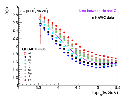
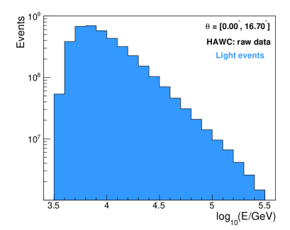
Figure 1: Left panel: Mean values of the expected age parameter for vertical EAS (circles) against the estimated shower energy for different primaries and for our nominal composition model (labelled as all, open squares). From above to below, the curves with circles correspond to Fe, Si, Mg, Ne, O, C, He and H, respectively. The HAWC data is also shown for comparison (solid squares). Errors on the mean are shown. The segmented line represents the $s_{He-C}$ cut. Right panel: The histogram of reconstructed energy for the measured sub-sample of light events obtained with the cut on the age parameter.

4 Reconstruction of the spectrum

The analysis employed in this work to estimate the spectrum of the light mass group of cosmic rays (H plus He nuclei) is simple and it can be summarized in the following way: First, we select a subset of data enriched with the primaries in which we are interested in. Then we build the energy distribution of the sub-sample and correct it for migration effects using an unfolding algorithm. Next, we correct the unfolded distribution for the contamination of heavy nuclei ($Z\geq 3$) and the efficiency for H+He primaries. Finally, from the result, we reconstruct the corresponding energy spectrum of the light mass group of cosmic rays.

Now, in order to select our light sub-sample from the data, we exploit the sensitivity of the age parameter to the primary composition. The latter is illustrated, in fig. 1, left, where the expected mean value of $s$ is presented as a function of the reconstructed energy for different cosmic ray species. The above plot shows that the age parameter increases with the mass of the primary nuclei and, in addition, decreases with $E$. This can be understood from the fact that light primaries and high energy cosmic rays produce air showers with $X_{max}$ closer to the ground and hence with steeper lateral distributions at detection level. To perform the selection, we apply a cut, $s_{He-C}$, on the data, located between the predicted curves for He and C (see fig. 1, left) in such a way that if the events satisfy $s<s_{He-C}$, then they are classified into the light mass group of cosmic rays, otherwise they are considered as a part of the heavy component. Using the above cut on the selected data, we are left with a sub-sample of $3.8\times 10^{9}$ events. In general, using MC simulations for our nominal composition model, we found out that the expected retention fraction of protons and helium nuclei in the light sub-sample is $\gtrsim 60$%, while its purity is $\gtrsim 90\%$.

After selecting our light sub-sample, we then build its corresponding energy histogram, $N_{light}^{raw}(E)$, using a bin size of $\Delta\log_{10}(E/\mbox{GeV})=0.1$ (see fig. 1, right). Then we apply the Bayes unfolding procedure [18] to correct this distribution for migration effects employing the response matrix, $P(E|E^{True})$ (c.f. fig. 2, left), which was derived for the light subset using MC simulations of our nominal composition model. Using the unfolded histogram $N_{light}^{Unf}(E^{True})$, the energy spectrum was calculated according to the following formula:

$$\Phi(E)=\frac{N_{light}^{Unf}(E^{True})}{\Delta E^{True}\mathcal{E}(E^{True})},$$ (2)

where $\Delta E^{True}$ is the width of the energy bin center at $E^{True}$ and $\mathcal{E}(E^{True})$ is the exposure, which is defined as:

$$\mathcal{E}(E^{True})=A_{eff}(E^{True})\cdot\Delta t_{eff}\cdot\Delta\Omega.$$ (3)

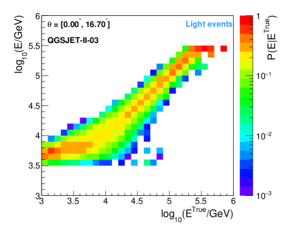
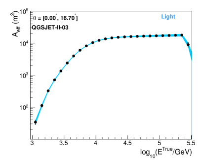
Figure 2: Left panel: The energy response matrix for the light sub-sample calculated from our nominal composition model. The vertical axis represent the reconstructed energy, and the horizontal axis, the true EAS energy. The color code indicates the probability $P(E|E^{True})$, which takes into account migration effects. Right panel: Effective area used for the calculation of the spectra for the H plus He mass group of cosmic rays. The curve was derived from MC simulations using our nominal composition model.

Here, $\Delta t_{eff}$ is the effective time of observation, $d\Omega$ is the differential solid angle and $A_{eff}(E^{True})$ is the effective area, which is defined as

$$\vspace{-0.5pc}A_{eff}(E^{True})=f_{corr}(E^{True})\cdot A^{H+He}_{eff}(E^{True})$$ (4)

with $A^{H+He}_{eff}$, the effective area of protons and helium nuclei in the light sub-sample and $f_{corr}$, a factor that corrects the spectrum for the presence of heavy elements in our data set with light events. Both $A^{H+He}_{eff}$ and $f_{corr}$ were estimated using MC simulations. In particular, the effective area was estimated from the expression below [7]:

$$A^{H+He}_{eff}(E^{True})=A_{thrown}\cdot\frac{\cos\theta_{max}+\cos\theta_{min}}{2}\cdot\epsilon^{H+He}(E^{True}),$$ (5)

where $A_{thrown}$ is the total throwing area of the MC events, $\theta_{min}$ and $\theta_{max}$ are the limits of the zenith angle interval considered in this study, and $\epsilon^{H+He}$ is the efficiency for detecting an hydrogen/helium-induced EAS and classifying it as a part of our light sub-sample. Meanwhile, $f_{corr}$ was calculated as the inverse of the expected fraction of H and He primaries in this sub-sample. The final result for $A_{eff}$ is shown in fig. 2, right, as a function of the primary energy. We see, from this plot that the maximum efficiency region is found between $\log_{10}(E/\mbox{GeV})=4$ and $5.3$. The drop at higher energies in the effective area is produced because we are running out of statistics there due to our selection cut at high energies. In the region of maximum efficiency, $f_{corr}$ decreases with energy from $1.13$ up to $1.06$.

Finally, the estimated energy spectrum of H plus He is presented in fig. 3, left, in the region of full efficiency. Here, the error bars represent the statistical errors and the error band, the systematic uncertainties. The first one varies between $1\%$ and $5\%$, while the second one, from $12.2\%$ to $17\%$. Statistical errors come from the data size of the sample and the limited statistics of the MC data used to estimate the response matrix. They were calculated according to [19]. Systematic errors include contributions from uncertainties in the primary composition (we used different composition models to reconstruct the spectrum), the calculation of the effective area, the position of the age cut (it was moved between the lines for He and C), the unfolding method (Gold’s unfolding [20] was also used and the initial spectrum as well as the regularization procedure were changed), the bin size, and the quantum efficiency/resolution of the PMTs.

The dominant source of systematic error in the procedure is the composition dependence of the response matrix and the effective area. The relative error of this systematic source varies in the range $11\%-15\%$. In order to evaluate this systematic error, we have estimated both $P(E|E_{True})$ and $A_{eff}$ using different models with distinct elemental abundances as predicted by the Polygonato model [21], and from fits to measurements from ATIC-2 [22], MUBEE [23] and JACEE [24], and then we have repeated the reconstruction procedure of the spectrum for each case. The variation among the different results including that one obtained using our nominal composition model was cited as the systematic error due to composition.

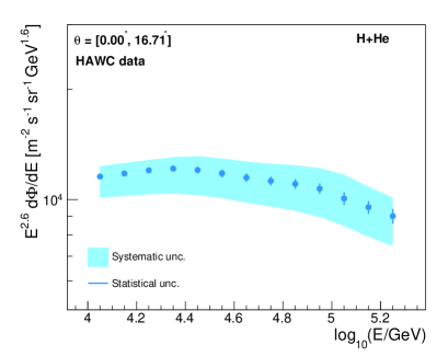
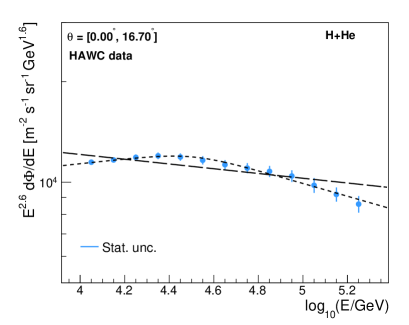
Figure 3: Left panel: The energy spectrum, multiplied by $E^{2.6}$, for the proton plus helium mass group of cosmic rays as measured with HAWC. The error bars represent statistical errors, while the error band, systematic uncertainties. Right panel: The results of the fit to the energy spectrum using a single power-law formula (long dashed line) and a double power-law function (short dashed line) as described in the text. Measured data is represented by data points. Error bars are statistical errors.

5 Discussion

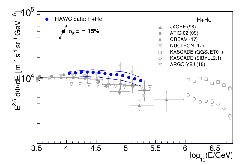
Figure 4: Left panel: The HAWC energy spectrum of protons plus helium nuclei (big blue circular points) is compared with measurements from direct (ATIC-2 [22], MUBEE [23] and NUCLEON [2]) and indirect (JACEE [24] and KASCADE [25]) experiments. In the HAWC data, statistical errors are smaller than the marker size. On the other hand, the error band represents the corresponding systematic uncertainty.

From figure fig. 3, left, we can observe that the spectrum for protons and helium nuclei seems to deviate from a single power-law behaviour. A $\chi^{2}$ fit with a single power-law expression,

$$\Phi(E)=\Phi_{0}E^{\gamma_{1}},$$ (6)

taking into account the correlations among the unfolded data points according to [26], gives $\gamma_{1}=-2.67\pm 0.01$ and $\log_{10}(\Phi_{0}/\mbox{m}^{-2}\mbox{s}^{-1}\mbox{sr}^{-1}\mbox{GeV}^{-1})=4.37\pm 0.04$ with $\chi^{2}=30.75$ for $N_{dof}=11$ degrees of freedom. On the other hand, a $\chi^{2}$ fit with a double power-law formula,

$$\Phi(E)=\Phi_{0}E^{\gamma_{1}}\left[1+\left(\frac{E}{E_{0}}\right)^{\xi}\right]^{(\gamma_{2}-\gamma_{1})/\xi},$$ (7)

provides the result $\gamma_{1}=-2.53\pm 0.05$, $\gamma_{2}=-2.79\pm 0.04$, $\log_{10}(\Phi_{0}/\mbox{m}^{-2}\mbox{s}^{-1}\mbox{sr}^{-1}\mbox{GeV}^{-1})=3.77\pm 0.23$ and $\log_{10}(E_{0}/\mbox{GeV})=4.50\pm 0.16$ with $\chi^{2}=1.16$ for $N_{dof}=8$ degrees of freedom. This result seems to imply the existence of a bending in the spectrum around $(3.2^{+1.4}_{-1.0})\times 10^{4}\,\mbox{GeV}$. The fitted functions are shown on fig. 3, right. In order to find out which hypothesis best describes the data, we used the test statistics $TS=\Delta\chi^{2}/\Delta N_{dof}$. First, by employing MC simulations, we generated different correlated data sets to calculate the distribution of $TS$ under the hypothesis of a single power-law behavior. From this distribution, we found a $p$-value $\leq 4.76\times 10^{-5}$ of having a $TS$ greater or equal the observed one ($TS_{obs}=9.86$). That implies a $3.90\,\sigma$ deviation from the scenario with a single power-law, which means that it is unlikely that the measured data is described by a single power-law function.

Finally, in fig. 4, we compare the HAWC spectrum for the light mass group of cosmic rays with the measurements from other experiments. We can see that the HAWC spectrum is above the measurements from the JACEE [24], ATIC-2 [22], CREAM-III [5] and ARGO-YBJ [3, 4] experiments, but it is in agreement with the NUCLEON results [2]. However, within total errors, at low energies HAWC seems to be in agreement with ATIC-2 and CREAM-III. We also note that the shape of the HAWC spectrum follows the same trend of the spectra measured by the above mentioned detectors above $10^{4}\,\mbox{GeV}$, but not that of ARGO-YBJ. Hence, HAWC may support previous observations by ATIC-2, CREAM-III and NUCLEON, which suggest the existence of a possible new feature in the spectrum of protons plus helium nuclei around a few $10\,\mbox{TeVs}$.

6 Conclusions

In the present study it was found that the lateral age parameter as measured with HAWC is sensitive to the composition of cosmic rays. By using such parameter and guided by MC simulations based on QGSJET-II-03, a sub-sample of HAWC data mainly composed by H and He nuclei was selected, from which the spectrum of the light component (H+He) of cosmic rays in the energy range from $10\,\mbox{TeV}$ to $200\,\mbox{TeV}$ was reconstructed. We have found that the spectrum of the protons plus helium in the cosmic ray flux measured with HAWC is not described by a single power-law function, but it seems to be in agreement with a double power-law behaviour. The fit of the data with the latter expression revels a change of the spectral index of the order of $\Delta\gamma=-0.26\pm 0.07$ in the H+He spectrum close to $(32^{+14}_{-10})\,\mbox{TeV}$. Further investigation is in progress to evaluate the impact of the high-energy interaction models in these results.

Acknowledgements The main list of acknowledgements can be found under the following link: https://www.hawc-observatory.org/collaboration/icrc2019.php. In addition, J.C.A.V. wants also to thank the partial support from CONACYT grant A1-S-46288.

References

- [1] T. Stanev et al., Front. Phys. 8 (2013) 748; T. Stanev et al., NIMA 742 (2014) 42.
- [2] E. Atkin et al., JCAP 1707 (2017) 020; E. Atkin et al. JETP Lett. 108 (2018) 5-12.
- [3] B. Bartoli et al., PRD 91, 112017 (2015).
- [4] B. Bartoli et al., PRD 92 (2015) 092005.
- [5] Y. S. Yoon et al., ApJ 839 (2017) 5.
- [6] A. U. Abeysekara et al., ApJ 843 (2017), 39.
- [7] R. Alfaro et al., PRD 96 (2017), 122001.
- [8] K. Kamata and J. Nishimura, Prog. of Theor. Phys. Supp. 6 (1958) 93.
- [9] A. U. Abeysekara et al., arXiv:1905.12518 [astro-ph.HE].
- [10] HAWC collaboration, J.A. Morales-Soto et al., PoS ICRC2019 (2019).
- [11] D. Heck et al., Report No. FZKA 6019, Forschungszentrum Karlsruhe-Wissenhaltliche Berichte (1998).
- [12] A. Ferrari, et al., CERN-2005-10 (2005), INFN/TC_05/11, SLAC-R-773; G. Battistoni et al., AIP Conf. Proc. 896 (2007) 31.
- [13] S. Ostapchenko, Phys. Rev. D 83 (2011) 014018.
- [14] M. Aguilar et al., PRL 114(17) (2015) 131103; PRL 115(21) (2015) 211101.
- [15] H. S. Ahn et al., ApJ 707 (2009) 593; APJ 728(2) (2011) 122.
- [16] O. Adriani et al., Science 332 (2011) 69.
- [17] S. Agostinelli et al., NIMA 506 (2003) 250.
- [18] G. D’Agostini, NIMA 362(2-3) (1995) 487.
- [19] T. Adye, arXiv:1105.1160 [physics.data-an]; T. Adye, Corrected error calculation for iterative Bayesian unfolding, http://hepunx.rl.ac.uk/ adye/software/unfold/bayes_errors.pdf.
- [20] R. Gold, Argonne National Laboratory Report ANL-6984, Argonne, 1964.
- [21] J. R. Hörandel, Astrop. Phys. 19(2) (2003) 193.
- [22] A. D. Panov et al., Bull. Russ. Acad. Sci. Phys. 71 (2007) 494.
- [23] V.I. Zatsepin et al., Proc. of the 23rd ICRC, editors: D.A. Leahy, R.B. Hickws, and D. Venkatesan, World Scientific, Vol. 2 (1993) 13.
- [24] Y. Takahashi et al., Nucl. Phys. B (Proc. Suppl.) 60B (1998) 83.
- [25] T. Antoni et al., Astrop. Phys. 24 (2005) 1.
- [26] G. Cowan, statistics review in M. Tanabashi et al. (PDG), PRD 98 (2018) 030001.