Cosmological studies from tomographic weak lensing peak abundances and impacts of photo-z errors
Abstract
Weak lensing peak abundance analyses have been applied in different surveys and demonstrated to be a powerful statistics in extracting cosmological information complementary to cosmic shear two-point correlation studies. Future large surveys with high number densities of galaxies enable tomographic peak analyses. Focusing on high peaks, we investigate quantitatively how the tomographic redshift binning can enhance the cosmological gains. We also perform detailed studies about the degradation of cosmological information due to photometric redshift (photo-z) errors. We show that for surveys with the number density of galaxies , the median redshift , and the survey area of , the 4-bin tomographic peak analyses can reduce the error contours of by a factor of comparing to 2-D peak analyses in the ideal case of photo-z error being absent. More redshift bins can hardly lead to significantly better constraints. The photo-z error model here is parametrized by and and the fiducial values of and is taken. We find that using tomographic peak analyses can constrain the photo-z errors simultaneously with cosmological parameters. For 4-bin analyses, we can obtain and without assuming priors on them. Accordingly, the cosmological constraints on and degrade by a factor of and , respectively, with respect to zero uncertainties on photo-z parameters. We find that the uncertainty of plays more significant roles in degrading the cosmological constraints than that of .
1 Introduction
Weak gravitational lensing (WL) effects have been shown to be a powerful probe in cosmological studies (Fu et al., 2008; Munshi et al., 2011; Heymans et al., 2013; Erben et al., 2013; Fu et al., 2014; Hildebrandt et al., 2017; Abbott et al., 2016; Hikage et al., 2019). Their high signals come dominantly from nonlinear regions of large-scale structures. Therefore to fully explore the cosmological information embedded in the WL data, different statistical analyses are needed. Besides cosmic shear two point correlation (2PCF) studies, WL peak abundance analyses have emerged to be an important statistics to extract cosmological information complementary to 2PCF (Shan et al., 2014; Liu et al., 2015b; Martinet et al., 2018; Shan et al., 2018; Liu et al., 2015a; Dietrich & Hartlap, 2010; Lin & Kilbinger, 2014).
Theoretically, WL effects depend on the formation and evolution of large-scale structures, and on the cosmic expansion history through the lensing efficiency kernel (Bartelmann & Schneider, 2001). Thus source galaxies at different redshifts experience different lensing effects, and tomographic analyses by dividing source galaxies into different redshift bins can significantly enhance the cosmological gains comparing to the 2-D studies without binning (Hu, 1999). Tomographic 2PCF analyses have been extensively studied and applied to different WL surveys (Fu et al., 2008; Erben et al., 2013; Hildebrandt et al., 2017; Abbott et al., 2016; Hikage et al., 2019). For WL peak statistics, limited to the relatively low number density of source galaxies from current surveys, tomographic studies have not been applied to WL data analyses. However, future large surveys will be able to produce much larger samples with the galaxy number reaching (LSST Science Collaboration et al., 2009; Zhan, 2011; Amendola et al., 2018; Hemmati et al., 2018), and thus enable the tomographic WL peak studies. From simulations, a number of studies have been carried out to explore the benefit of employing tomographic WL peak analyses (Dietrich & Hartlap 2010; Lin & Kilbinger 2014; Liu et al. 2015a; Petri et al. 2016; Martinet et al. 2018; Li et al. 2018; Price et al. 2018).
For WL surveys, practically, the galaxy redshifts can only be derived from multi-band photometric observations. Such photometric redshifts (photo-z) inevitably have errors. Therefore for tomographic WL analyses, to assess the impacts of photo-z errors on the derived cosmological constraints is crucially important. From these studies, we can also set requirements for the accuracy of photo-z estimates and the subsequent calibrations (Ma et al., 2006; Huterer et al., 2006; Ma & Bernstein, 2008; Amara & Réfrégier, 2008; Sun et al., 2009; Bernstein & Huterer, 2010; Hearin et al., 2010, 2012; Yao et al., 2017; Cao et al., 2018). While the impacts of the photo-z errors on the tomographic 2PCF have been systematically studied in depth (Ma & Bernstein, 2008; Mandelbaum et al., 2008; Hemmati et al., 2018), similar analyses for WL peak statistics are still lacking. In Abruzzo & Haiman (2018), they investigated the influences of photo-z errors on tomographic peak analyses from simulations. In their studies, the cosmology dependence of peak abundances is solely from simulations spanning a range of cosmological parameters. Thus for each value of photo-z errors, a separate WL simulation is needed for each of the cosmological models considered. It is therefore not easy for them to study the capability of using tomographic analyses to constrain the photo-z error parameters simultaneously with cosmological parameters, and the corresponding degradations on cosmological constraints and the requirements for the prior knowledge on photo-z errors. Instead, they studied the cosmological parameter bias induced from different photo-z biases, and used the B/U ratio (bias vs. statistical uncertainty) for a cosmological parameter as an estimate for its degradation factor.
In this paper, we carry out the studies on tomographic peak analyses. We focus on high WL peaks, and employ our theoretical model of Yuan et al. (2018) for calculating the cosmological dependence of tomographic peak abundances. This model is an extension of the model of Fan et al. (2010) and includes both the shape noise and the projection of large-scale structures into consideration. With this theoretical basis, we are able to investigate the cosmological gains of different redshift binning of tomographic peak analyses and the impact of the photo-z errors. For the latter, we investigate the capability of simultaneously constraining the photo-z error parameters and the cosmological parameters using tomographic peak abundance data, and the degradation of the cosmological constraints due to the propagation of photo-z errors into the uncertainties of cosmological parameters . We then further examine the requirements of the prior knowledge on the photo-z error parameters with respect to the degradation requirements. To facilitate and validate our analyses, we also use large ray tracing simulations to generate mock data taking into account the photo-z errors in our studies.
The rest of the paper is organized as follows. In Sec.2, we summarize our theoretical model of Yuan et al. (2018) for high WL peak abundances. In Sec.3, we describe our simulations. In Sec. 4, we show the cosmological gains of tomographic peak analyses with different redshift binnings in the ideal case without photo-z errors. We present our detailed analyses on the impact of photo-z errors in Sec.5. Conclusions and discussions are shown in Sec. 6.
2 THE MODEL FOR WEAK LENSING HIGH PEAK ABUNDANCES
The WL effect arises from the light deflection by large-scale structures in the Universe. The induced observational effects can be described by the second derivatives of the lensing potential , i.e., the Jacobin matrix given by (Bartelmann & Schneider, 2001):
| (1) |
where
| (2) |
with being the two-dimensional angular vector.
The convergence , reflecting the isotropic change of a background image, is related to the projected density fluctuation weighted by the lensing kernel under the Born approximation, and thus can intuitively reveal the (dark) matter distribution in the Universe. The components lead to anisotropic shears to an image. Observationally, WL signals are extracted by measuring accurately the shapes of background galaxies, and thus statistically directly related to the reduced shear defined as . Because of the physical relation between and , the convergence field can be reconstructed from the galaxy shape measurements, which inevitably includes the contamination from the shape noise resulting from the intrinsic ellipticities of source galaxies. We can also construct a scalar aperture mass field directly from the reduced shears, and thus avoiding the possible artificial effects from the reconstructions. In WL lensing regime with , and , the field is approximately the same as the convergence field convolved with a compensated filter.
In this study, we aim to analyze the benefit from tomographic WL peak analyses, and how the photo-z errors affect the cosmological studies. For that, we concentrate on high peaks in the convergence field smoothed with a Gaussian kernel. We note, however, that the peak model to be described is also applicable to the convergence field filtered by compensated kernels (Yuan et al., 2018). Moreover, following the same halo approach, we have developed a theoretical model for high peaks in constructed directly from the reduced shear field, and the results agree with that from simulations very well (Pan et al. in preparation). Therefore the methodologies shown in this paper can be readily extended to investigate tomographic peaks.
For a high convergence peak, studies have shown that its signal is typically dominated by the contribution from a single massive halo along the line of sight (Hamana et al., 2004; Yang et al., 2011; Liu & Haiman, 2016; Wei et al., 2018). This leads to the halo-based model of Fan et al. (2010) for WL high peaks, in which the Gaussian shape noise is taken into account. In Yuan et al. (2018), we extended the model by further including the projection effect from large-scale structures in the calculation. This improvement is important because future surveys will go deeper and thus the projection effect can be comparable to that from the shape noise. In this model, we consider halo regions and the field region, separately. In halo regions, the smoothed convergence field can be written as
| (3) |
where is the contribution from massive halos with mass larger than , is the contribution from the projection effect of large-scale structures excluding those from the massive halos already considered, and is from the shape noise. Both and are modeled as Gaussian random fields. For the shape noise field , the moments are given by
| (4) |
with being the power spectrum of the smoothed noise field. For , we have
| (5) |
where the power spectrum is calculated by
| (6) |
where is the cosmic scale factor, and is the lensing kernel function
| (7) |
Here is the source redshift distribution function. For , in Yuan et al., 2018, it is modeled by subtracting the one halo term from massive halos with mass above the threshold from the full non-linear power spectrum, i.e., (For more details please see Eq.(18)-Eq.(23) in Yuan et al. 2018.)
| (8) |
Finally for the combined Gaussian random field, its moments are given by
| (9) |
Then for an individual halo region, we can calculate the peak distribution using the Gaussian random field theory modulated by the halo profile (Fan et al., 2010). It is noted that in this region, it contains the peak corresponding to the original halo peak but the position and the height are changed due to the existence of the combined Gaussian random field. It also has peaks from the Gaussian random field with the heights modulated by the halo profile. For peaks in all the massive halo regions, we integrate over the massive halos with the number weighted by the halo mass function.
The field region corresponds to regions outside halos considered above. In this region, the peak distribution can be calculated from the combined Gaussian random field without halo modulations. The total peak abundance is then computed by the summation of peaks in halo regions and that in the field region (Yuan et al., 2018).
In the next section, we describe our tomographic simulations, and also compare the simulation results with the model predictions to validate the applicability of the model to tomographic WL peak analyses.
3 Simulated convergence maps
The same 24 sets of -body simulation data as in Liu et al., 2015b and in Yuan et al., 2018 are used here. They are under the flat CDM model with the cosmological parameters = (0.28, 0.72, 0.046, 0.7, 0.96, 0.82). Each set consists of 12 independent simulation boxes, with 8 having the box size of 320 and the particle number of to fill the region from to , and 4 larger ones with the same particle number but the size of 600 for the region with . From each set of simulations, the WL ray tracing calculations are done using 59 lens planes up to . For each plane, we store the convergence and shear data computed from the lens planes before it. The convergence maps with different redshift distributions can then be constructed from these 59 maps by weighting each plane according to the considered source redshift distribution function . Specifically to generate 2-D convergence maps without tomography, we use,
| (10) |
where is the normalization factor for . In this paper, we adopt the overall redshift distribution as follows (LSST Science Collaboration et al., 2009)
| (11) |
from to and mimicking the LSST-like surveys. From each of the 24 sets of simulations, we can obtain 4 maps each with the area of deg2 pixelized into data points. Thus totally we have deg2 convergence data for each redshift distribution considered. We then add the Gaussian shape noise to each pixel according to
| (12) |
where we take . It is noted that this is the dispersion of the total ellipticities including two components. Its value is related to both the intrinsic ellipticity distribution of source galaxies, and the galaxy shape measurement errors. The value of taken here is in accord with that of CFHTLenS observations (Kilbinger et al., 2013). And the pixel size of maps arcmin. In the 2-D case, the source galaxy number density is taken to be 40 arcmin-2. We then apply a Gaussian smoothing with the kernel given by
| (13) |
We take = 2.0 arcmin to obtain the final smoothed noisy convergence maps.
From the smoothed convergence maps, we identify peaks if their convergence values are larger than those of the surrounding 8 pixels. Then we record the peak height scaled by the shape noise . To avoid the possible boundary effects on the smoothed maps, we exclude the outer 70 pixels along each side of a map, which corresponds to about in the peak analyses. Thus the total effective area used in our analyses is about 876 deg2.
To simulate the tomographic convergence maps, in the ideal case without photo-z errors, we divide the source galaxies into different bins. For the bin with , the and used in Eq.(10) and Eq.(12) are computed by
| (14) |
and
| (15) |
The corresponding normalization factor is .
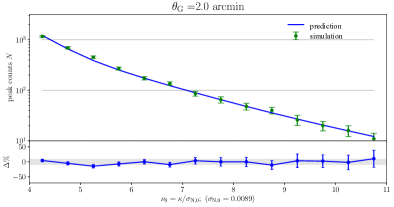
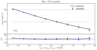
In Fig.1, we show the peak abundances in the 2-D case. The blue line is our theoretical prediction, and the green points with error bars are from simulations. For illustration purposes, the error bars here show the Poisson errors for the number of peaks in different bins in the total simulated area of , without considering the covariance between different bins. In the later cosmological analyses in this work, we take into account the full covariance. The lower panel shows the relative differences between the results from the model and the simulation. The gray areas indicate the % range.
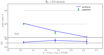
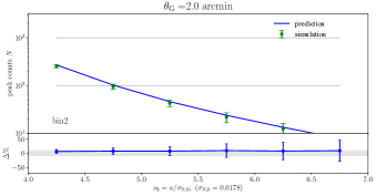
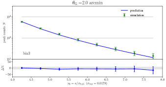
Similarly, in Fig.2, we present the 4-bin tomographic results where the redshift binning is defined so that the number density of source galaxies in each bin is the same with 10 arcmin-2. It is seen that our model predictions agree with simulation results very well both in the 2-D case and in the tomographic peak calculations.
With photometric redshift errors, to generate the tomographic convergence maps based on the photo-z binning, we need to first calculate the corresponding true redshift distribution for a particular photo-z bin. Following Ma et al. (2006), the photometric redshift () distribution given a true redshift is modeled by
| (16) |
where the redshift-dependent bias and the scatter are given by and with and being constants. With this model, the true redshift distribution in the photo-z bin of is
| (17) |
which gives
| (18) |
4 THE DEPENDENCE OF COSMOLOGICAL GAINS ON THE NUMBER OF REDSHIFT BINS
In this section, we investigate the optimal redshift binning in tomographic high WL peak studies with respect to the cosmological information enhancement. Here we consider the ideal case without photo-z errors. Intuitively, more redshift bins can provide more information about the evolution of large-scale structures, and thus increase the gains. However, given a survey, the number of galaxies per bin decreases with the increase of bin numbers, and the statistical uncertainties increase correspondingly. Therefore there should exist an optimal range of bins for cosmological studies. For tomographic 2PCF analyses, it is found that typically 5-10 bins give best cosmological constraints, and a further increase of the number of bins cannot lead to significant improvements (Hearin et al., 2012; Ma et al., 2006).
Here we study how the number of redshift bins affects the cosmological constraints from tomographic high WL peak analyses. For that, we consider and 8, respectively. For each , we construct a set of tomographic convergence maps as described in Sec. 3. From these maps, we identify peaks with and then group them to obtain the peak abundances in different bins with the width of . We then calculate the covariance of the peak abundances for an area of (excluding the outer 70 pixels in each side) from the 96 maps, and scale the covariance to the considered area.
It is known that the constraints from WL analyses generally show a banana shape. When the survey area is relatively small, this deviates from an ellipse considerably, indicating that the Fisher matrix analyses can lead to some errors (Vallisneri, 2008; Perotto et al., 2006; Sellentin et al., 2014; Sellentin & Schäfer, 2016; Brinckmann & Lesgourgues, 2019). Thus in this section to perform cosmological studies with different , we do not use the Fisher matrix forecast. Instead, we carry out more general MCMC fitting. In the next section to investigate the impact of photo-z errors, we focus on a large survey area of 15000 . For that, the expected statistical errors are small. We thus apply the Fisher analyses there, which should be applicable to a high degree and are more efficient than MCMC fitting when photo-z error parameters are also included in the study.
We adopt the same likelihood analysis procedures as in Yuan et al. 2018. The is defined as:
| (19) |
where with being the mock data vector of WL peak counts of different bins and being the theoretical predictions for these bins. For the covariance, in this paper, we first calculate them directly from simulated maps for an area of , denoted as . For that, for each of the 96 maps, we generate 20 shape noises with different random seeds. Thus we totally have maps. From them, we compute the covariance matrix of peaks. For the covariance of a large area , we use the scaling relation of . It is noted that this scaling does not include contributions to the covariance from scales larger than . Thus it can lead to a slight underestimate of the covariance for an area of (Kratochvil et al., 2010; Liu et al., 2015b). For more precise analyses, we need to run many large simulations to produce many maps matching the considered survey area to calculate the covariance matrix. This can be difficult. Certain approximated and fast simulation methods have been proposed (Fluri et al., 2018). The full analyses of the covariance calculations are beyond the scope of the current paper, and will be studied in our future investigations.
To calculate the inverse covariance, we adopt the unbiased estimator used in Hartlap et al. (2007), which is given by
| (20) |
where and is the number of bins of WL peak counts used in deriving cosmological constraints, and is the normal inverse of .
From Fig.1 and Fig.2, we see that our theoretical model for high WL peak abundances works very well. Thus for clarity, in this section, we perform cosmological parameter forecasts for different values of with mock observational data generated directly from our model calculations and the covariance from simulations. Here we consider the survey area of , the same as the effective area of our simulations. The improvement on the cosmological information gains from tomographic peak analyses is evaluated by comparing the derived constraints with that from the 2-D peak analyses.
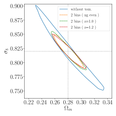
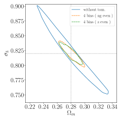
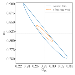
In Fig.3, we show the 1- confidence regions of for different cases. In all the panels, the blue contour is from the 2-D peak analyses. The left panel shows the results of , where three different binning methods are considered. The orange one is from dividing galaxies into two equal-number-density bins, and the green and red ones are using and as a dividing point, respectively. The middle panel is for the results of with the orange contour from the equal-number-density binning and the green one from the equal-z-interval binning, respectively. The right panel is for , and only the result from the equal-number-density binning is shown. By comparing with the blue contour in each panel, we see very clearly that tomographic peak analyses can indeed enhance the cosmological information significantly. The improvement from to is apparent. However, for , the constraint is nearly the same as that of .
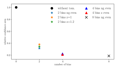
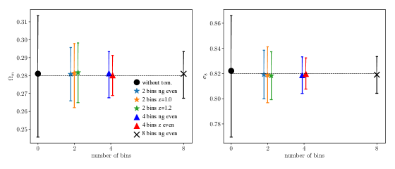
To be more quantitative, we calculate the area within 1- confidence region in different cases, and the results relative to the 2-D case are shown in the upper panel of Fig.4. It is seen that from 2-D to , the constraining area is reduced by about 2.5 times, which is about 40% of that of the 2-D case without tomography. With , the area further decreases by about a factor of two. Further to the improvement is not significant. In the lower panels of Fig.4, we show the comparisons of the corresponding 1-D constraints for (left) and (right). The trend is the same as that shown in the upper panel.
We thus conclude that considering high WL peaks, with the source redshift distribution similar to LSST, tomographic peak analyses with can give optimal cosmological constraints, which can improve the 1- confidence area of by a factor of 5 with respect to the 2-D peak analyses without redshift binning. To increase the number of bins further cannot lead to significantly better constraints.
5 IMPACT OF PHOTOMETRIC REDSHIFT ACCURACY ON TOMOGRAPHIC PEAK ANALYSES
In Sec.4, we studied the cosmological information improvement from tomographic peak analyses in the ideal case that the galaxy redshifts are perfectly known. In practice, however, for WL cosmological studies, we need to observe a large number of far-way source galaxies that are typically faint. It is therefore very difficult to obtain spectroscopic redshifts (spec-z) for all the galaxies. The feasible way is to estimate their photo-z by multi-band observations. The accuracy of photo-z depends on observations, such as the overall wavelength coverage, the central position and band-width of filters, photometric accuracy, etc., as well as the methodology for photo-z estimates (Hildebrandt et al., 2010; Salvato et al., 2019).
The photo-z errors are often characterized by the bias, the scatter, and the fraction of outliers, estimated using a subsample of galaxies with known spec-z (Salvato et al., 2019). It is noted that not only these information, but also their uncertainties, namely, errors on errors, are important in tomographic WL studies. Their effects on tomographic 2PCF analyses and the corresponding error propagation to cosmological studies have been investigated extensively (Ma et al., 2006; Huterer et al., 2006; Ma & Bernstein, 2008; Amara & Réfrégier, 2008; Sun et al., 2009; Bernstein & Huterer, 2010; Hearin et al., 2010, 2012; Yao et al., 2017). For WL peak studies, some of the photo-z effects are explored using numerical simulations (Petri et al., 2016; Abruzzo & Haiman, 2018).
In this section, the impacts of photo-z errors on tomographic high WL peak studies are analyzed. We investigate how the photo-z error parameters can be constrained simultaneously with cosmological parameters, and the corresponding degradations of the cosmological constraints. We then study how the knowledge about photo-z errors on errors can improve the degradations. Here we consider the survey area of 15000 , and adopt the Fisher forecast approach to efficiently explore the multi-dimensional parameter space.
5.1 Photometric redshift errors
For easy-read purposes, we list the photo-z relevant formulae again here. The photo-z distribution given a true redshift is taken to be Gaussian, given by
| (21) |
where and are the redshift-dependent scatter (precision) and bias with and being constants to be constrained and analyzed from tomographic peak abundances. Then the true redshift distribution given the photometric redshift interval can be calculated to be
| (22) |
In the Fisher analyses here, we adopt the photo-z error parameters as that required by LSST-like surveys, with the fiducial vales of and respectively. The overall true redshift distribution is given by Eq.(11). Meanwhile we scale the covariance calculated from our mock simulations to the survey area of 15000 . Note that in this study, we do not consider catastrophic photo-z errors with large deviations from the true redshifts that cannot be described by Eq.(21) (Sun et al., 2009).
The following two cases are considered including the photo-z errors:
-
1.
2-bins-tomography divided by photometric redshift =1.0;
-
2.
4-bins-tomography divided by even source galaxies number density adopt from photometric redshift.
In our model calculations, we include the photo-z error parameters by adopting the distribution of Eq.(22). The likelihood is then updated to include four free parameters to be constrained simultaneously.
5.2 Fisher analyses and error propagation
In the Fisher approximation, the error propagation from data to cosmological parameters can be estimated by the Fisher matrix given by: (Ma et al., 2006; Heavens, 2016)
| (23) |
where are the parameters to be constrained. Assuming Gaussian priors for both and , their prior matrix can be written as
| (24) |
where the and are the standard dispersions of the corresponding Gaussian priors. According to the Bayesian theory, the Fisher matrix of posterior is:
| (25) |
This is used to forecast the parameter constraints by computing its inverse matrix as follows
| (26) |
To calculate the Fisher matrix Eq.(23), because we have our theoretical model for tomographic high peak abundances, in principle, we can compute the derivatives directly from the model. However, such estimates can suffer from numerical instabilities. To avoid these, we run MCMC fitting for the case without any priors on the photo-z error parameters. From the converged sampling chains, we obtain an estimate for the corresponding covariance by
| (27) |
where denotes the point in the four-dimensional parameter space at the -th sampling step and is the number of total steps in MCMC chains and are the mean values obtained from the MCMC chains. Its inverse matrix gives rise to an estimation of the Fisher matrix corresponding to Eq.(23) without the photo-z priors, which is given by
5.3 High peak tomography with photometric redshift errors
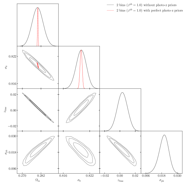
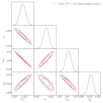
We first study the 2-bin case with the dividing redshift set to be . In Fig.5, we show the constraining results without priors on photo-z error parameters obtained from MCMC fitting (black contours). For comparison, the cosmological parameter constraints with perfectly known photo-z errors, i.e., fixing their values to the fiducial ones with and , are also shown in the figure (in red). It is seen from the black contours that, in the 2-bin case, there are strong degeneracies between the photo-z error parameters and the cosmological parameters. This leads to a severe degradation in cosmological parameter constraints if no prior knowledge on the photo-z error parameters is known.
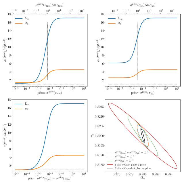
We then add different priors to the photo-z parameters to study the improvements in the cosmological parameter constraints. The results are shown in Fig.6. The first and the second panels are for the results adding the prior only to or , respectively, leaving the other one fully free without prior. The vertical axes are the degradation factor with respect to the case with perfectly known and . We also show the degradation by assuming equal priors on and , i.e., , in the lower left panel. The lower right panel is for the cosmological constraints of with a few examples of different priors on the photo-z parameters. From the plots, we see clearly that the error on photo-z bias parameter affects more importantly in the cosmological constraints than that of scatter parameter . Without any prior on , the degradations on the cosmological parameters are if the prior on can reach the level of . However, in the case that is completely free from any prior, the best degradations we can get for and are and , respectively, even with the prior on reaching zero. The vertical dotted lines in the first and the second panels indicate the location where the prior is equal to the constraint shown by the corresponding black line in Fig.5 obtained solely from the 2-bin tomographic peak abundances without any priors on photo-z parameters.
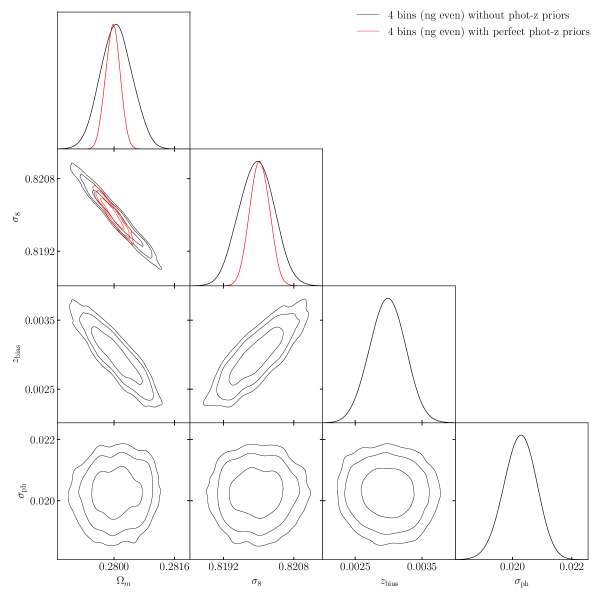
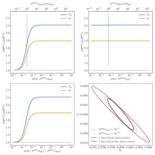
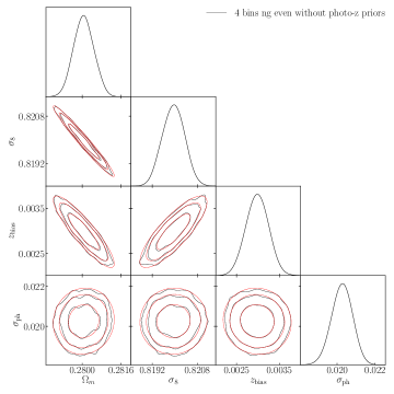
Now we show the results for the 4-bin case with equal number density of source galaxies in each bin. The parameter forecasts for models with free parameters of (black) and the case with fixed and (red) are shown Fig.7. Similar to the 2-bin case, without any priors on the photo-z parameters, the information of cosmological parameters is also degraded, but the level is smaller than that of the 2-bin case. We also see that with 4-bin tomographic peak abundances, we can constrain and much better than that of the 2-bin case. There is still an apparent degeneracy between the cosmological parameters and , but their correlations with are insignificant. The degradation curves and 1- contours for different priors on the photo-z parameters are shown in Fig.8. It is seen that adding prior on alone has nearly no impact on the degradation on cosmological parameter constraints (upper right panel). On the other hand, if we control the prior on to the precision of without any prior on , the degradation factors can be close to unit (upper left panel). This is consistent with the degeneracy behaviors shown in Fig.7.
Comparing the degradation curves of the above 2 cases (the upper left and the upper right panels in Fig.6 and Fig.8), we find that the prior on the bias parameter is more important for improving the cosmological information gain. From the lower left panel of Fig.6 and Fig.8, it is seen that the results are about the same as those applying priors only to , which demonstrate again the importance of knowing accurately.
To see the dependence of the degradation factors on the priors of and more clearly, we use the Sherman–Morrison formula, which shows that the inverse of and defined in Eq.(25) are related by:
| (29) |
If only the prior on parameter is considered, the posterior error of the other parameters can be computed from the diagonal elements of left hand side of Eq.(29) (For details please see Eq.(3) – Eq.(10) in Amendola & Sellentin, 2016.), which is
| (30) |
where and are the standard dispersion obtained without any priors, and is the correlation coefficient between the two parameters (without any priors added as well). The quantity is the dispersion from the posterior distribution defined in Eq.(25) including the a prior with a dispersion of on parameter .
We can see that the effect of the prior of on the constraint of the parameter depends on their correlation , the larger the correlation, the stronger the effect. The correlation coefficients between different parameters in the 2-bin and 4-bin cases are shown in Table.1. It is seen that in the 4-bin case, the correlations between and the other parameters are very small, thus its prior has almost no effect on the degradation factors of and as seen in the upper right panel of Fig.8. On the other hand, the correlations between and the cosmological parameters are large, therefore the prior on is much more important in improving the degradations than that of .
| 1 | -0.966 | -0.997 | 0.944 | |
| -0.974 | -0.891 | 0.060 | ||
| 1 | 0.947 | -0.824 | ||
| 0.826 | 0.031 | |||
| 1 | -0.947 | |||
| 0.045 | ||||
| 1 |
5.4 Photo-z calibration requirements
In this study, we assume a Gaussian-like conditional probability of photo-z given a spec-z, with the bias and the dispersion being and , respectively. We analyze the dependence of the degradation of the cosmological constraints on the priors of the two error parameters , and show that the prior knowledge on the bias parameter plays more important roles in improving the cosmological information gain.
Observationally, one direct way to calibrate the conditional probability of photo-z is to use a number of spec-z measurements. Assuming we have spec-z in the a photo-z bin centered at and a bin width , and they are fair samples of the Gaussian distribution. Then the accuracies of the estimates about and are (Ma et al., 2006)
| (31) | ||||
It is noted that the factor occurs in both sides of the equations, and thus can be canceled out. They give an estimate about the required number in each bin given a desired prior on the photo-z errors. The dashed and solid black lines in Fig.9 shows the above relations taking .
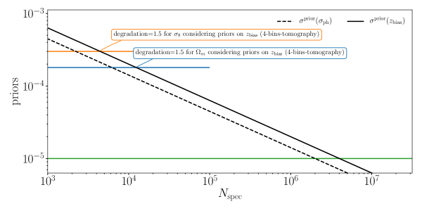
For the 4-bin tomographic peak studies, with , there is nearly no degradation in cosmological parameter constraints comparing to the case with perfectly known photo-z parameters. To reach this accuracy, is needed for each redshift bin. We note that here should be smaller than the bins used for tomographic peak analyses so that the a single Gaussian distribution centered on is applicable. With , and the source redshifts extending to , we need totally spec-z measurements. This can be a challenge, particularly for high redshift bins. If we allow a factor of 1.5 degradation in the cosmological parameter constraints, in the 4-bin case, the photo-z accuracy can be relaxed to . The corresponding requirements for spec-z observations is in each bin. We caution here that the Gaussian conditional photo-z distribution with the form of bias and the dispersion considered in this paper is relatively simple. More generally, the photo-z errors in different bins can be different, and not follow the dependence. In that case, we need to include more photo-z error parameters, and the prior requirements for different photo-z bins can be different. This can affect the requirements on the number of spec-z observations (Ma et al., 2006).
In addition to the direct spec-z calibration, variety of other photo-z calibration methods have been discussed in literature (Salvato et al., 2019). The detailed tomographic WL peak studies taking into account complicated photo-z distributions and careful examinations of the requirements for different redshift calibration methods are beyond the scope of the current paper, and will be addressed in our future investigations.
6 Conclusions
In this paper, we investigate the potential of tomographic WL peak abundance studies, and explore the cosmological gains from the peak tomography in comparison with that of 2-D peak statistics. We concentrate on high peaks with signal-to-noise ratio , and adopt our theoretical model to calculate the fiducial peak abundances in different tomographic bins. At the same time, we carry out ray-tracing simulations to validate our model, and also to compute the covariance matrix for tomographic peak statistics.
Considering LSST-like surveys, we find that 4-bin tomographic peak analyses can lead to about 5 times better constraints for and than that from 2-D peak abundances in the ideal case without considering photo-z errors. Taking into account these errors, we investigate how they can be constrained simultaneously with cosmological parameters using tomographic peak abundances alone. Adopting a Gaussian conditional photo-z distribution with the bias and the dispersion modeled as and , respectively, we show that 4-bin peak tomography itself can constrain photo-z error parameters to the level of , and . The corresponding cosmological constraints for and are degradated by a factor of 2.2 and 1.8, respectively, with respect to the case with perfectly known and . To limit the degradation to below 1.5, we need to have a prior knowledge on z bias with the accuracy of . The priors on are less important.
Intuitively, the more sensitive dependence of tomographic peak analyses on than on can be understood as follow. The peak number counts depend on the redshift through the lensing kernel, the redshift dependence of the mass function, and the angular size of massive halos. If there is a in the photo-z measurements, it affects the peak counts in a systematic way. Over (under) estimate the photo-z will lead to under (over) estimate of . This leads to a very sensitive dependence on for tomographic peak statistics. On the other hand, for the dispersion , to the linear order, we can write the peak count near as . Thus the change on the peak count from the plus and minus parts cancels out. In this case, we expect that the dependence of peak counts on is minimal. In reality, there are higher order terms of in the expansion beyond the linear term, thus the canceling is partial. The smaller the , the more canceling occurs. In our 2-bin analyses, the constraint on purely from the peak counts is relatively large, and we still see a certain dependence on the priors of for the tomographic peak studies (top right panel of Fig.6). In the 4-bin case, the peak count data themselves can give already a tight constraint on , and thus the canceling discussed above is more complete. Thus there is nearly no dependence on the priors of for the peak analyses (top right panel of Fig.8). Similarly, the more sensitive dependence on than on also shows up in the tomographic two point correlation analyses (Ma et al., 2006; Huterer et al., 2006).
The requirements on the photo-z calibrations using spec-z are also discussed. For the 4-bin case with the degradation factor of , we need , which in turn requires in each redshift calibration bin for the fiducial . We note that the calibration requirements depend on the assumed photo-z distributions. More realistic photo-z distributions taking into account the redshift dependence of their error parameters beyond assumption may result better estimates about the desired accuracy of photo-z error parameters, and thus more realistic requirements about the spec-z measurements. Other redshift calibration methods are also worth to be explored. Particularly, for some surveys, such as Euclid111https://www.euclid-ec.org/ and Chinese Space Station Telescope (CSST) (Zhan, 2011, 2018; Fan, 2018), they will have both imaging surveys and slitless spectroscopic surveys. Detailed studies on how their spec-z sample can help the photo-z calibration for the WL galaxy sample, both in terms of direct calibrations and using the correlation methods, are needed in order to fully explore their cosmological potentials. For that, specific survey characteristics and the error budget should be taken into account in the analyses.
In this paper, we focus on photo-z errors. There are also other sources of systematics that can affect weak lensing peak studies. Among these, galaxy intrinsic alignments can have significant effects. They not only can generate additional shape noise (Fan, 2007), but also can affect the peak signals from clusters of galaxies. The latter is related to the level of cluster member contaminations to the source galaxies and their alignments in the host clusters. In addition, the uncertainties of dark matter halo properties, such as the halo mass function and the halo density profiles and their triaxialities (Tang & Fan, 2005), and the baryonic effects (Fong et al., 2019; Weiss et al., 2019), etc., can also induce systematic errors in cosmological studies from weak lensing peak statistics. Importantly, these effects can degenerate to some degree with the effects of photo-z errors. For comprehensive understandings of these effects, much more detailed investigations taking into account different systematics are needed, which will be the major efforts in our future studies.
Appendix A The Gaussian approximation for likelihoods
In Sec.5.4, we employ the Fisher approximation to study how the photo-z errors affect the tomographic WL peak analyses and the derived cosmological constraints. Here in Fig.10, we show the comparisons of the MCMC results (black) and those from Fisher approximation (red) for the 2-bin and 4-bin cases considered in Sec.5.4. It is seen that in both cases, the constraints from the Fisher approximation agree excellently with those from MCMC fitting, showing its validity in our forecast studies assuming LSST-like survey parameters.
References
- Abbott et al. (2016) Abbott, T., Abdalla, F. B., Allam, S., et al. 2016, Phys. Rev. D, 94, 022001
- Abruzzo & Haiman (2018) Abruzzo, M. W., & Haiman, Z. 2018, arXiv e-prints, arXiv:1810.12312
- Amara & Réfrégier (2008) Amara, A., & Réfrégier, A. 2008, MNRAS, 391, 228
- Amendola & Sellentin (2016) Amendola, L., & Sellentin, E. 2016, MNRAS, 457, 1490
- Amendola et al. (2018) Amendola, L., Appleby, S., Avgoustidis, A., et al. 2018, Living Reviews in Relativity, 21, 2
- Bartelmann & Schneider (2001) Bartelmann, M., & Schneider, P. 2001, Phys. Rep., 340, 291
- Bernstein & Huterer (2010) Bernstein, G., & Huterer, D. 2010, MNRAS, 401, 1399
- Brinckmann & Lesgourgues (2019) Brinckmann, T., & Lesgourgues, J. 2019, Physics of the Dark Universe, 24, 100260
- Cao et al. (2018) Cao, Y., Gong, Y., Meng, X.-M., et al. 2018, MNRAS, 480, 2178
- Dietrich & Hartlap (2010) Dietrich, J. P., & Hartlap, J. 2010, MNRAS, 402, 1049
- Erben et al. (2013) Erben, T., Hildebrandt, H., Miller, L., et al. 2013, MNRAS, 433, 2545
- Fan (2018) Fan, Z. 2018, in COSPAR Meeting, Vol. 42, 42nd COSPAR Scientific Assembly, E1.16–9–18
- Fan et al. (2010) Fan, Z., Shan, H., & Liu, J. 2010, ApJ, 719, 1408
- Fan (2007) Fan, Z. H. 2007, ApJ, 669, 10
- Fluri et al. (2018) Fluri, J., Kacprzak, T., Sgier, R., Refregier, A., & Amara, A. 2018, J. Cosmology Astropart. Phys, 2018, 051
- Fong et al. (2019) Fong, M., Choi, M., Catlett, V., et al. 2019, MNRAS, 1821
- Fu et al. (2008) Fu, L., Semboloni, E., Hoekstra, H., et al. 2008, A&A, 479, 9
- Fu et al. (2014) Fu, L., Kilbinger, M., Erben, T., et al. 2014, MNRAS, 441, 2725
- Hamana et al. (2004) Hamana, T., Takada, M., & Yoshida, N. 2004, MNRAS, 350, 893
- Hartlap et al. (2007) Hartlap, J., Simon, P., & Schneider, P. 2007, A&A, 464, 399
- Hearin et al. (2012) Hearin, A. P., Zentner, A. R., & Ma, Z. 2012, Journal of Cosmology and Astro-Particle Physics, 2012, 034
- Hearin et al. (2010) Hearin, A. P., Zentner, A. R., Ma, Z., & Huterer, D. 2010, ApJ, 720, 1351
- Heavens (2016) Heavens, A. 2016, Entropy, 18, 236
- Hemmati et al. (2018) Hemmati, S., Capak, P., Masters, D., et al. 2018, arXiv e-prints, arXiv:1808.10458
- Heymans et al. (2013) Heymans, C., Grocutt, E., Heavens, A., et al. 2013, MNRAS, 432, 2433
- Hikage et al. (2019) Hikage, C., Oguri, M., Hamana, T., et al. 2019, Publications of the Astronomical Society of Japan, 22
- Hildebrandt et al. (2010) Hildebrandt, H., Arnouts, S., Capak, P., et al. 2010, A&A, 523, A31
- Hildebrandt et al. (2017) Hildebrandt, H., Viola, M., Heymans, C., et al. 2017, MNRAS, 465, 1454
- Hu (1999) Hu, W. 1999, ApJ, 522, L21
- Huterer et al. (2006) Huterer, D., Takada, M., Bernstein, G., & Jain, B. 2006, MNRAS, 366, 101
- Kilbinger et al. (2013) Kilbinger, M., Fu, L., Heymans, C., et al. 2013, MNRAS, 430, 2200
- Kratochvil et al. (2010) Kratochvil, J. M., Haiman, Z., & May, M. 2010, Phys. Rev. D, 81, 043519
- Li et al. (2018) Li, Z., Liu, J., Zorrilla Matilla, J. M., & Coulton, W. R. 2018, arXiv e-prints, arXiv:1810.01781
- Lin & Kilbinger (2014) Lin, C.-A., & Kilbinger, M. 2014, in IAU Symposium, Vol. 306, Statistical Challenges in 21st Century Cosmology, ed. A. Heavens, J.-L. Starck, & A. Krone-Martins, 107–109
- Liu & Haiman (2016) Liu, J., & Haiman, Z. 2016, Phys. Rev. D, 94, 043533
- Liu et al. (2015a) Liu, J., Petri, A., Haiman, Z., et al. 2015a, Phys. Rev. D, 91, 063507
- Liu et al. (2015b) Liu, X., Pan, C., Li, R., et al. 2015b, MNRAS, 450, 2888
- LSST Science Collaboration et al. (2009) LSST Science Collaboration, Abell, P. A., Allison, J., et al. 2009, arXiv e-prints, arXiv:0912.0201
- Ma & Bernstein (2008) Ma, Z., & Bernstein, G. 2008, ApJ, 682, 39
- Ma et al. (2006) Ma, Z., Hu, W., & Huterer, D. 2006, ApJ, 636, 21
- Mandelbaum et al. (2008) Mandelbaum, R., Seljak, U., Hirata, C. M., et al. 2008, MNRAS, 386, 781
- Martinet et al. (2018) Martinet, N., Schneider, P., Hildebrandt, H., et al. 2018, MNRAS, 474, 712
- Munshi et al. (2011) Munshi, D., Heavens, A., & Coles, P. 2011, MNRAS, 411, 2161
- Perotto et al. (2006) Perotto, L., Lesgourgues, J., Hannestad, S., Tu, H., & Y Y Wong, Y. 2006, Journal of Cosmology and Astro-Particle Physics, 2006, 013
- Petri et al. (2016) Petri, A., May, M., & Haiman, Z. 2016, Phys. Rev. D, 94, 063534
- Price et al. (2018) Price, M. A., Cai, X., McEwen, J. D., & Kitching, T. D. 2018, arXiv e-prints, arXiv:1812.04018
- Salvato et al. (2019) Salvato, M., Ilbert, O., & Hoyle, B. 2019, Nature Astronomy, 3, 212
- Sellentin et al. (2014) Sellentin, E., Quartin, M., & Amendola, L. 2014, MNRAS, 441, 1831
- Sellentin & Schäfer (2016) Sellentin, E., & Schäfer, B. M. 2016, MNRAS, 456, 1645
- Shan et al. (2018) Shan, H., Liu, X., Hildebrandt, H., et al. 2018, MNRAS, 474, 1116
- Shan et al. (2014) Shan, H. Y., Kneib, J.-P., Comparat, J., et al. 2014, MNRAS, 442, 2534
- Sun et al. (2009) Sun, L., Fan, Z.-H., Tao, C., et al. 2009, ApJ, 699, 958
- Tang & Fan (2005) Tang, J. Y., & Fan, Z. H. 2005, ApJ, 635, 60
- Vallisneri (2008) Vallisneri, M. 2008, Phys. Rev. D, 77, 042001
- Wei et al. (2018) Wei, C., Li, G., Kang, X., et al. 2018, MNRAS, 478, 2987
- Weiss et al. (2019) Weiss, A. J., Schneider, A., Sgier, R., et al. 2019, arXiv e-prints, arXiv:1905.11636
- Yang et al. (2011) Yang, X., Kratochvil, J. M., Wang, S., et al. 2011, Phys. Rev. D, 84, 043529
- Yao et al. (2017) Yao, J., Ishak, M., Lin, W., & Troxel, M. 2017, Journal of Cosmology and Astro-Particle Physics, 2017, 056
- Yuan et al. (2018) Yuan, S., Liu, X., Pan, C., Wang, Q., & Fan, Z. 2018, ApJ, 857, 112
- Zhan (2011) Zhan, H. 2011, Scientia Sinica Physica, Mechanica & Astronomica, 41, 1441
- Zhan (2018) Zhan, H. 2018, in COSPAR Meeting, Vol. 42, 42nd COSPAR Scientific Assembly, E1.16–4–18