Anderson Accelerated Douglas–Rachford SplittingThe work of the first and second authors was each supported by a Stanford Graduate Fellowship.

Abstract

We consider the problem of nonsmooth convex optimization with linear equality constraints, where the objective function is only accessible through its proximal operator. This problem arises in many different fields such as statistical learning, computational imaging, telecommunications, and optimal control. To solve it, we propose an Anderson accelerated Douglas–Rachford splitting (A2DR) algorithm, which we show either globally converges or provides a certificate of infeasibility/unboundedness under very mild conditions. Applied to a block separable objective, A2DR partially decouples so that its steps may be carried out in parallel, yielding an algorithm that is fast and scalable to multiple processors. We describe an open-source implementation and demonstrate its performance on a wide range of examples.

49J52, 65K05, 68W10, 68W15, 90C25, 90C53, 97N80

10.1137/19M1290097

1 Introduction

1.1 Problem setting

Consider the convex optimization problem

(1) $$\begin{array}[]{ll}\text{minimize}&f(x)\\ \text{subject to}&Ax=b\end{array}$$

with variable $x\in{\mbox{\bf R}}^{n}$, where $f:{\mbox{\bf R}}^{n}\rightarrow{\mbox{\bf R}}\cup\{+\infty\}$ is convex, closed, and proper (CCP), and $A\in{\mbox{\bf R}}^{m\times n}$ and $b\in{\mbox{\bf R}}^{m}$ are given. We assume that the linear constraint $Ax=b$ is feasible.

Block form

In this paper, we work with block separable $f$, i.e., $f(x)=\sum_{i=1}^{N}f_{i}(x_{i})$ for individually CCP $f_{i}:{\mbox{\bf R}}^{n_{i}}\rightarrow{\mbox{\bf R}}\cup\{+\infty\}$, $i=1,\dots,N$. We partition $x=(x_{1},\dots,x_{N})$ so that $n=\sum_{i=1}^{N}n_{i}$ and let $A=[A_{1}~{}A_{2}~{}\cdots~{}A_{N}]$ with $A_{i}\in{\mbox{\bf R}}^{m\times n_{i}}$, $i=1,\dots,N$. Problem (1) can be written in terms of the block variables as

(2) $$\begin{array}[]{ll}\text{minimize}&\sum_{i=1}^{N}f_{i}(x_{i})\\ \text{subject to}&\sum_{i=1}^{N}A_{i}x_{i}=b.\end{array}$$

Many interesting problems have the form (2), such as consensus optimization [10] and cone programming [35]. In fact, by transforming nonlinear convex constraints (e.g., cone constraints) into set indicator functions and adding them to the objective function, any convex optimization problem can be written in the above form.

Optimality conditions

The point $x\in{\mbox{\bf R}}^{n}$ is a solution to (2) if there exist $g\in{\mbox{\bf R}}^{n}$ and $\lambda\in{\mbox{\bf R}}^{m}$ such that

(3) $$Ax=b,$$

(4) $$0=g+A^{T}\lambda,\quad g\in\partial f(x),$$

where $\partial f(x)$ is the subdifferential of $f$ at $x$. With block separability, (4) can be written as

$$0=g_{i}+A_{i}^{T}\lambda,\quad g_{i}\in\partial f_{i}(x_{i}),\quad i=1,\dots,N.$$

We refer to (3) and (4) as the primal feasibility and dual feasibility conditions, and $x$ and $\lambda$ as the primal variable and dual variable, respectively. Together, these conditions are sufficient for optimality; they become necessary as well when Slater’s constraint qualification is satisfied, i.e., $\mathop{\bf relint}\mathop{\bf dom}f\cap\{x\,:\,Ax=b\}\neq\emptyset$.

Proximal oracle

Methods for solving (2) vary depending on what oracle is available for $f_{i}$. If $f_{i}$ and its subgradient can be queried directly, a variety of iterative algorithms may be used [11, 34, 33]. However, in our setting, we assume that each $f_{i}$ can only be accessed through its proximal operator ${\mathop{\textbf{prox}}}_{tf_{i}}:{\mbox{\bf R}}^{n_{i}}\rightarrow{\mbox{\bf R}}^{n_{i}}$, defined as

$${\mathop{\textbf{prox}}}_{tf_{i}}(v_{i})=\mathop{\rm argmin}\nolimits_{x_{i}}~{}\left(f_{i}(x_{i})+\tfrac{1}{2t}\|x_{i}-v_{i}\|_{2}^{2}\right),$$

where $t>0$ is a parameter. In particular, we assume neither direct access to the function $f_{i}$ nor its subdifferential $\partial f_{i}$. The separability of $f$ implies that [39]

$${\mathop{\textbf{prox}}}_{tf}(v)=\left({\mathop{\textbf{prox}}}_{tf_{1}}(v_{1}),\dots,{\mathop{\textbf{prox}}}_{tf_{N}}(v_{N})\right)$$

for any $v=(v_{1},\dots,v_{N})\in{\mbox{\bf R}}^{n}$.

While we cannot evaluate $\partial f_{i}$ at a general point, we can find an element of $\partial f_{i}$ at the proximal operator’s image point:

$$x_{i}={\mathop{\textbf{prox}}}_{tf_{i}}(v_{i})\Longleftrightarrow 0\in\partial f_{i}(x_{i})+\tfrac{1}{t}(x_{i}-v_{i})\Longleftrightarrow\tfrac{1}{t}(v_{i}-x_{i})\in\partial f_{i}(x_{i}).$$

Thus, by querying the proximal oracle of $f_{i}$ at $v_{i}$, we obtain an element in the subgradient of $f_{i}$ at $x_{i}={\mathop{\textbf{prox}}}_{tf_{i}}(v_{i})$.

The optimality conditions can be expressed using the proximal operator as well. The point $x\in{\mbox{\bf R}}^{n}$ is a solution to (2) if there exist $v\in{\mbox{\bf R}}^{n}$ and $\lambda\in{\mbox{\bf R}}^{m}$ such that

(5) $$Ax=b,$$

(6) $$0=\tfrac{1}{t}(v-x)+A^{T}\lambda,\quad x_{i}={\mathop{\textbf{prox}}}_{tf_{i}}(v_{i}),\quad i=1,\dots,N.$$

Residuals

From conditions (5) and (6), we define the primal and dual residuals at $x,\lambda$ as

(7) $$r_{\rm{prim}}=Ax-b,$$

(8) $$r_{\rm{dual}}=\tfrac{1}{t}(v-x)+A^{T}\lambda,$$

and we define the overall residual as $r=(r_{\rm prim},r_{\rm dual})\in{\mbox{\bf R}}^{n+m}$.

Stopping criterion

If problem (2) is feasible and bounded, a reasonable stopping criterion is that the residual norm lies below some threshold, i.e., $\|r\|_{2}\leq\epsilon_{\rm tol}$, where $\epsilon_{\rm tol}>0$ is a user-specified tolerance. We refer to the associated $x$ as an approximate solution to (2). We defer discussion of the criteria for pathological (infeasible/unbounded) cases to section 4.

Notice that given a candidate $v\in{\mbox{\bf R}}^{n}$, we can readily choose the primal point $x={\mathop{\textbf{prox}}}_{tf}(v)$ and dual point

(9) $$\lambda=\tfrac{1}{t}(A^{\dagger})^{T}(x-v)\in\mathop{\rm argmin}\nolimits_{\hat{\lambda}}~{}\|A^{T}\hat{\lambda}-\tfrac{1}{t}(x-v)\|_{2},$$

a minimizer of the dual residual norm, where $A^{\dagger}$ denotes the pseudoinverse of $A$. Thus, any algorithm for solving (2) via the proximal oracle need only determine a $v$ that produces a small residual norm.

1.2 Related work

When functional access is restricted to a proximal oracle, the most common approaches for solving (2) are the alternating direction method of multipliers (ADMM) [56, 38, 18, 6], Douglas–Rachford splitting (DRS) [22], and the augmented Lagrangian method [64] with appropriate problem reformulations (e.g., consensus). These algorithms take advantage of the separability of the objective function, making them well-suited for the nonsmooth convex optimization problem considered in this paper. Yet despite their robustness and scalability, they typically suffer from slow convergence. Researchers have proposed several acceleration techniques, including adaptive penalty parameters [21, 60], adaptive synchronization [9], and momentum methods [63]. In practice, improvement from these techniques is usually limited due to the first-order nature of the accelerated algorithms. Special cases of (2) can sometimes yield exploitable problem forms, such as the Laplacian regularized stratified model in [54]. There the authors use the structure of the Laplacian matrix to efficiently parallelize ADMM. However, for the general problem, further acceleration requires a quasi-Newton method with line search [51] or semismooth Newton method with access to the Clarke’s generalized Jacobian of the objective’s proximal operator [4, 59, 31], both of which typically impose high per-iteration costs and memory requirements.

The acceleration technique adopted in this paper, type-II Anderson acceleration (AA), dates back to the 1960s [5]. It belongs to the family of sequence acceleration methods, which achieve faster convergence through certain sequence transformations. The origin of these methods can be traced to Euler’s transformation of series [1] from the 18th century. Several faster sequence acceleration techniques were proposed in the 20th century, including Aitken’s $\Delta^{2}$-process in 1926 [3] along with its higher-order [47, 57] and vector [30, 28, 48] extensions, of which AA is a member. We refer readers to [12, 7] for a thorough history. AA can be viewed as either an extrapolation method or a generalized quasi-Newton method [17]. However, unlike classical quasi-Newton methods, it is effective without a line search and requires less computation and memory per iteration so long as certain stabilization measures are adopted.

Type-II AA was initially proposed to accelerate solvers for nonlinear integral equations in computational chemistry and materials science; later, it was applied to general fixed-point problems [55]. It operates by using an affine combination of previous iterates to determine the next iterate of an algorithm, where the combination’s coefficients are obtained by solving an unconstrained least squares problem. In this sense, it is a generalization of the averaged iteration algorithm and Nesterov’s accelerated gradient method. Its local convergence properties have been analyzed in a range of settings, both deterministic [42, 53, 46, 16, 25, 29, 41] and stochastic [45, 52], but its global convergence properties remain largely unknown except for a variant called EDIIS [24]. EDIIS has been shown to converge globally assuming that the fixed-point mapping is contractive [13]. However, it adds nonnegativity constraints to the coefficients of AA, meaning each iteration must solve a nonnegative least squares problem, a more complex task than solving the unconstrained problem, which admits a closed-form solution. The technique proposed in this paper, by contrast, only requires nonexpansiveness for global convergence. Each of its iterations merely solves an unconstrained least squares problem, similar to the original type-II AA. Recently, [17] proposed another AA variant called type-I AA. While less stable than its type-II counterpart, this variant performs more favorably with appropriate stabilization and globalization [36, 61].

AA has been applied in the literature to several problems related to (2). The authors of [40] use AA to speed up a parallelized local-global solver for geometry optimization and physics simulation problems, which may be viewed as a special case of our problem where $f_{i}$ are projection operators. In a separate setting, [27] employs AA to solve large-scale fixed-point problems arising from partial differential equations, demonstrating performance improvements on a distributed memory platform. More generally, [61] uses type-I AA in conjunction with DRS and a splitting conic solver (SCS) [35] to solve problems in consensus and conic optimization. These results are extended by [49], which combines type-II AA with an SCS variant to produce SuperSCS, an efficient solver for large cone programs. AA has also seen success in nonconvex settings. Notably, [62] applies AA to ADMM and studies its empirical performance on nonconvex optimization problems arising in computer graphics.

1.3 Contribution

In this paper, we consider the DRS algorithm for solving (2), which satisfies the proximal oracle assumption and admits a simple fixed-point (FP) formulation [43]. This FP format allows us to improve the convergence of DRS with AA, a memory efficient, line search free acceleration method that works on generic nonsmooth, nonexpansive FP mappings with almost no extra cost per iteration [61]. Motivated by the need for solver stability, we choose type-II AA in our current work and propose a robust stabilization scheme that maintains its speed and efficiency. We then apply it to DRS and show that the resulting Anderson accelerated Douglas–Rachford splitting (A2DR) algorithm always either converges or provides a certificate of infeasibility/unboundedness under very relaxed conditions. As a consequence, we obtain the first globally convergent type-II AA variant in nonsmooth, potentially pathological settings. Our convergence analysis only requires nonexpansiveness of the FP mapping, gracefully handling cases when a fixed-point does not exist. Finally, we release an open-source Python solver based on A2DR at

https://github.com/cvxgrp/a2dr.

Outline

We begin in section 2 by introducing the basics of DRS. We then describe AA and propose A2DR in section 3. The global convergence properties of A2DR are established in section 4, along with an analysis of the infeasible and unbounded cases. We discuss the presolve, equilibration, and hyperparameter choices in section 5, followed by the implementation details in section 6. In section 7, we demonstrate the performance of A2DR on several examples. We conclude in section 8.

2 Douglas–Rachford splitting

Douglas–Rachford splitting (DRS) is an algorithm for solving problems of the form

$$\mbox{minimize}\quad g(x)+h(x)$$

with variable $x$, where $g$ and $h$ are CCP [43]. We can write problem (2) in this form by taking $g=f$ and $h=\mathcal{I}_{\{x\,:\,Ax=b\}}$, the indicator function of the linear equality constraint. Notice that ${\mathop{\textbf{prox}}}_{th}$ is the projection onto the associated subspace, defined as

$$\Pi(v^{k+1/2})=v^{k+1/2}-A^{\dagger}(Av^{k+1/2}-b)=v^{k+1/2}-A^{T}(AA^{T})^{\dagger}(Av^{k+1/2}-b).$$

The DRS algorithm proceeds as follows.

Algorithm 1 Douglas–Rachford Splitting (DRS)

1:Input: initial point $v^{0}$, penalty coefficient $t>0$.

2:for $k=1,2,\dots$ do

3:     $x^{k+1/2}={\mathop{\textbf{prox}}}_{tf}(v^{k})$

4:     $v^{k+1/2}=2x^{k+1/2}-v^{k}$

5:     $x^{k+1}=\Pi(v^{k+1/2})$

6:     $v^{k+1}=v^{k}+x^{k+1}-x^{k+1/2}$

7:end for

Each iteration $k$ requires the evaluation of the proximal operator of $f$ and the projection onto a linear subspace.

Dual variable and residuals

We regard $x^{k+1/2}$, the proximal operator’s image point, as our approximate primal optimal variable in iteration $k$. There are two ways to produce an approximate dual variable $\lambda^{k}$. The first way sets

$$\lambda^{k}=\tfrac{1}{t}(AA^{T})^{\dagger}(Av^{k+1/2}-b),$$

an intermediate value from the projection step. (See Remark A.3 in the supplementary materials for the reasoning behind this choice.) The second way computes $\lambda^{k}$ as the minimizer of $\|r_{\rm dual}^{k}\|_{2}$, which necessitates solving the least squares problem (9) at each iteration. Our implementation uses the second method because the additional computational cost is minimal, and this choice of a dual optimal variable results in earlier stopping.

The primal and dual residuals can be calculated by plugging our DRS iterates into (7) and (8):

(10) $$r_{\rm prim}^{k}=Ax^{k+1/2}-b,$$

(11) $$r_{\rm dual}^{k}=\tfrac{1}{t}(v^{k}-x^{k+1/2})+A^{T}\lambda^{k}.$$

Convergence

Define the fixed-point mapping $F_{\text{DRS}}:{\mbox{\bf R}}^{n}\rightarrow{\mbox{\bf R}}^{n}$ as

$$F_{\text{DRS}}(v)=v+\Pi\left(2\textbf{prox}_{tf}(v)-v\right)-\textbf{prox}_{tf}(v),$$

so that $v^{k+1}=F_{\text{DRS}}(v^{k})$. It can be shown that $F_{\rm DRS}$ is $1/2$-averaged (i.e., $F_{\rm DRS}=\frac{1}{2}H+\frac{1}{2}I$, where $H$ is nonexpansive and $I$ is the identity mapping), and hence, $v^{k}$ converges globally and sublinearly to a fixed-point of $F_{\rm DRS}$ whenever such a point exists. In this case, $x^{k+1/2}$ and $x^{k+1}$ both converge to a solution of (2), implying that $\lim_{k\rightarrow\infty}\|r_{\rm prim}^{k}\|_{2}=\lim_{k\rightarrow\infty}\|r_{\rm dual}^{k}\|_{2}=0$ [43].

3 Anderson accelerated DRS

In this section, we give a brief overview of AA and propose a modification that improves its stability. We then combine stabilized AA with DRS to construct our main algorithm, Anderson accelerated DRS. A2DR always produces an approximate solution to (2) when the problem is feasible and bounded. We treat the infeasible/unbounded cases in section 4.

3.1 Anderson acceleration

Consider a $1/2$-averaged mapping $F:{\mbox{\bf R}}^{n}\rightarrow{\mbox{\bf R}}^{n}$. To solve the associated fixed-point problem $F(v)=v$, we can repeatedly apply the fixed-point iteration (FPI) $v^{k+1}=F(v^{k})$, which is exactly DRS when $F=F_{\rm DRS}$. However, convergence of FPI algorithms is usually slow in practice. Acceleration schemes are one way of addressing this flaw. AA is a special form of the generalized limited-memory quasi-Newton (LM-QN) method. It is one of the most successful acceleration schemes for general nonsmooth FPIs, exhibiting greater memory efficiency than classical LM-QN algorithms like the restarted Broyden’s method [49].

We focus here on the original type-II AA [5]. Let $G(v)=v-F(v)$ be the residual function and $M^{k}\in\mathbf{Z}_{+}$ a nonnegative integer denoting the memory size. Typically, $M^{k}=\min(M_{\max},k)$ for some maximum memory $M_{\max}\geq 1$ [55]. At iteration $k$, type-II AA stores in memory the most recent $M^{k}+1$ iterates $(v^{k},\dots,v^{k-M^{k}})$ and replaces $v^{k+1}=F(v^{k})$ with $v^{k+1}=\sum_{j=0}^{M^{k}}\alpha_{j}^{k}F(v^{k-M^{k}+j})$, where $\alpha^{k}=(\alpha_{0}^{k},\dots,\alpha_{M^{k}}^{k})$ is the solution to

(12) $$\begin{array}[]{ll}\mbox{minimize}&\|\sum_{j=0}^{M^{k}}\alpha_{j}^{k}G(v^{k-M^{k}+j})\|_{2}^{2}\\ \mbox{subject to}&\sum_{j=0}^{M^{k}}\alpha_{j}^{k}=1.\end{array}$$

AA then updates its memory to $(v^{k+1},\dots,v^{k+1-M^{k+1}})$ before repeating the process.

The accelerated $v^{k+1}$ can be seen as an extrapolation from the original $v^{k+1}$ and the fixed-point mappings of a few earlier iterates. It has the potential to reduce the residual by a significant amount. In particular, when $F$ is affine, (12) seeks an affine combination $\tilde{v}^{k+1}$ of the last $M^{k}+1$ iterates that minimizes the residual norm $\|G(\tilde{v}^{k+1})\|_{2}$, then computes $v^{k+1}=F(\tilde{v}^{k+1})$ by performing an additional FPI.

3.2 Main algorithm

Despite the popularity of type-II AA, it suffers from instability in its original form [46]. We propose a stabilized variant using adaptive regularization and a simple safeguarding globalization trick.

Adaptive regularization

Define $g^{k}=G(v^{k})$, $y^{k}=g^{k+1}-g^{k}$, $s^{k}=v^{k+1}-v^{k}$, $Y_{k}=[y^{k-M^{k}}~{}\cdots~{}y^{k-1}]$, and $S_{k}=[s^{k-M^{k}}~{}\cdots~{}s^{k-1}]$. With a change of variables, (12) can be rewritten as [55]

(13) $$\mbox{minimize}\quad\|g^{k}-Y_{k}\gamma^{k}\|_{2}$$

with respect to $\gamma^{k}=(\gamma_{0}^{k},\dots,\gamma_{M^{k}-1}^{k})$, where

(14) $$\alpha_{0}^{k}=\gamma_{0}^{k},\quad\alpha_{i}^{k}=\gamma_{i}^{k}-\gamma_{i-1}^{k},\quad i=1,\ldots,M^{k}-1,\quad\alpha_{M^{k}}^{k}=1-\gamma_{M^{k}-1}^{k}.$$

To improve stability, we add an $\ell_{2}$-regularization term to (13), scaled by the Frobenius norms of $S_{k}$ and $Y_{k}$, which yields the problem

(15) $$\begin{array}[]{ll}\text{minimize}&\|g^{k}-Y_{k}\gamma^{k}\|_{2}^{2}+\eta\left(\|S_{k}\|_{F}^{2}+\|Y_{k}\|_{F}^{2}\right)\|\gamma^{k}\|_{2}^{2},\end{array}$$

where $\eta>0$ is a parameter. The regularization adopted in (15) differs from the one introduced in [46] that directly regularizes $\alpha^{k}$. We argue that with the affine constraint on $\alpha^{k}$, it is more natural to regularize the unconstrained variables $\gamma^{k}$. This approach also allows us to establish global convergence in section 4. Intuitively, if the algorithm is converging, $\lim_{k\rightarrow\infty}\|S_{k}\|_{F}=\lim_{k\rightarrow\infty}\|Y_{k}\|_{F}=0$, so the coefficient on the regularization term vanishes just like in the single iteration local analysis by [46].

A simple and relaxed safeguard

To achieve global convergence, we also need a safeguarding step. This step checks whether the current residual norm is sufficiently small. If true, the algorithm takes the AA update and skips the safeguarding check for the next $R-1$ iterations. Otherwise, the algorithm replaces the AA update with the vanilla FPI update. Here $R\in\mathbf{Z}_{++}$ is a positive integer that determines the degree of safeguarding; smaller values are more conservative, since the safeguarding step is performed more often.

A$2$DR

We are finally ready to present A2DR (Algorithm 2). A2DR applies type-II AA with adaptive regularization (lines 10–11) and safeguarding (lines 13–17) to the DRS fixed-point mapping $F_{\rm DRS}$. In our description, $G_{\rm DRS}=I-F_{\rm DRS}$ is the residual mapping, $D>0,~{}\epsilon>0$ are constants that characterize the degree of safeguarding, and $n_{\rm AA}^{k}$ is the number of times the $AA$ candidate has passed the safeguarding check up to iteration $k$.

Stopping criterion

As explained in section 1, to check optimality, we evaluate the primal and dual residuals $r_{\rm prim}^{k}$ and $r_{\rm dual}^{k}$. We terminate the algorithm and output $x^{k+1/2}$ as the approximate solution if

(16) $$\|r^{k}\|_{2}\leq\epsilon_{\rm tol}=\epsilon_{\rm abs}+\epsilon_{\rm rel}\|r^{0}\|_{2},$$

where $r^{k}=(r_{\rm prim}^{k},r_{\rm dual}^{k})$ and $\epsilon_{\rm abs}>0,\epsilon_{\rm rel}>0$ are user-specified absolute and relative tolerances, respectively.

Algorithm 2 Anderson Accelerated Douglas–Rachford Splitting (A2DR)

1:Input: initial point $v^{0}$, penalty coefficient $t>0$, regularization coefficient $\eta>0$, safeguarding constants $D>0,~{}\epsilon>0,~{}R\in\mathbf{Z}_{++}$, max-memory $M_{\max}\in\mathbf{Z}_{+}$.

2:Initialize $n_{\rm AA}=0,~{}R_{\rm AA}=0,~{}I_{\text{safeguard}}=\texttt{True}$.

3:Compute $v^{1}=F_{\rm DRS}(v^{0})$, $g^{0}=v^{0}-v^{1}$.

4:for $k=1,2,\dots$ do

5:     # Memory update

6:     Choose memory $M^{k}=\min(M_{\max},k)$.

7:     Compute the DRS candidate: $v_{\rm DRS}^{k+1}=F_{\rm DRS}(v^{k})$, $g^{k}=v^{k}-v^{k+1}_{\rm DRS}$.

8:     Update $Y_{k}$ and $S_{k}$ with $y^{k-1}=g^{k}-g^{k-1}$ and $s^{k-1}=v^{k}-v^{k-1}$.

9:     # Adaptive regularization

10:     Solve for $\gamma^{k}$ in regularized least squares (15) and compute weights $\alpha^{k}$ from (14).

11:     Compute the AA candidate: $v_{\rm AA}^{k+1}=\sum_{j=0}^{M^{k}}\alpha_{j}^{k}v_{\rm DRS}^{k-M^{k}+j+1}$.

12:     # Safeguard

13:     If $I_{\text{safeguard}}$ is True or $R_{\rm AA}\geq R$:

14:           If $\|g^{k}\|_{2}=\|G_{\rm DRS}(v^{k})\|_{2}\leq D\|g^{0}\|_{2}(n_{\rm AA}/R+1)^{-(1+\epsilon)}$:

15:                 $v^{k+1}=v_{\rm AA}^{k+1}$, $n_{\rm AA}=n_{\rm AA}+1$, $I_{\text{safeguard}}=\texttt{False}$, $R_{\rm AA}=1$.

16:           else $v^{k+1}=v_{\rm DRS}^{k+1}$, $R_{\rm AA}=0$.

17:     else $v^{k+1}=v_{\rm AA}^{k+1}$, $n_{\rm AA}=n_{\rm AA}+1$, $R_{\rm AA}=R_{\rm AA}+1$.

18:     Terminate and output $x^{k+1/2}$ (cf. Algorithm 1) if stopping criterion (16) is satisfied.

19:end for

4 Global convergence

We now establish the global convergence properties of A2DR. In particular, we show that under the general assumptions in section 1, A2DR either converges globally from any initial point or provides a certificate of infeasibility/unboundedness.

4.1 Infeasibility and unboundedness

When the optimality conditions do not hold even in the asymptotic sense, i.e., if the infimum of the primal or dual residual over all possible $x$ and $v$ is nonzero, problem (2) is either infeasible or unbounded. We say that (2) is infeasible if $\mathop{\bf dom}f\cap\{x\,:\,Ax=b\}=\emptyset$, and we say that it is unbounded if (2) is feasible, but $\inf_{Ax=b}f(x)=-\infty$. The following proposition characterizes sufficient certificates of infeasibility and unboundedness.

Proposition 4.1 (certificates of infeasibility and unboundedness).

Let $f^{*}:{\mbox{\bf R}}^{n}\rightarrow{\mbox{\bf R}}\cup\{+\infty\}$ denote the conjugate function of $f$, defined as $f^{*}(y)=\sup\nolimits_{x\in\mathop{\bf dom}f}\big{(}y^{T}x-f(x)\big{)}$.

1. If $\mathop{\bf dist{}}(\mathop{\bf dom}f,\,\{x\,:\,Ax=b\})>0$, then problem (2) is infeasible.

2. If $\mathop{\bf dist{}}(\mathop{\bf dom}f^{*},\,\mathop{\bf range}(A^{T}))>0$, then problem (2) is unbounded.

When (i) holds, (2) is also called (primal) strongly infeasible, and when (ii) holds, (2) is called dual strongly infeasible [26]. We say that (2) is pathological if it is either primal or dual strongly infeasible, and solvable otherwise. Notice that when the problem is pathological, it is either infeasible or unbounded, but not both.

Proof 4.2.

Claim (i) is true by definition. To prove claim (ii), observe that the dual problem of (2) is $\text{minimize}_{\nu}~{}f^{*}(\nu)+g^{*}(-\nu)$, where $g^{*}(\nu)=b^{T}\lambda$ when $\nu=A^{T}\lambda$, and $g^{*}(\nu)=+\infty$ otherwise. By Lemma 1 in [44], if $\mathop{\bf dist{}}(\mathop{\bf dom}f^{*},\,\mathop{\bf range}(A^{T}))>0$, then the dual problem is strongly infeasible, and hence the primal problem (2) is unbounded.

If (2) is pathological, an algorithm should provide a certificate of either (i) or (ii). We will show that A2DR achieves this goal by returning the distances in (i) and (ii) as a by-product of its iterations.

4.2 Convergence results

We are now ready to present the convergence results for A2DR. We begin by highlighting the contribution of adaptive regularization to the stabilization of AA. Indeed, by setting the gradient of the objective function in (15) to zero, we find the solution is

$$\gamma^{k}=(Y_{k}^{T}Y_{k}+\eta\left(\|S_{k}\|_{F}^{2}+\|Y_{k}\|_{F}^{2}\right)I)^{-1}Y_{k}^{T}g^{k}.$$

Using the relationship between $\alpha^{k}$ and $\gamma^{k}$, we then write

(17) $$\begin{split}v^{k+1}&=v^{k}-(I+(S_{k}-Y_{k})(Y_{k}^{T}Y_{k}+\eta\left(\|S_{k}\|_{F}^{2}+\|Y_{k}\|_{F}^{2}\right)I)^{-1}Y_{k}^{T})g^{k}=v^{k}-H_{k}g^{k},\end{split}$$

where $H_{k}=I+(S_{k}-Y_{k})(Y_{k}^{T}Y_{k}+\eta\left(\|S_{k}\|_{F}^{2}+\|Y_{k}\|_{F}^{2}\right)I)^{-1}Y_{k}^{T}$.

Lemma 4.3.

The matrices $H_{k}$ ($k\geq 0$) satisfy $\|H_{k}\|_{2}\leq 1+2/\eta$.

Proof 4.4.

Since $\|A\|_{2}\leq\|A\|_{F}$ for any matrix $A$,

$$\begin{split}\|H_{k}\|_{2}&\leq 1+\dfrac{\|S_{k}-Y_{k}\|_{2}\|Y_{k}\|_{2}}{\eta\left(\|S_{k}\|_{F}^{2}+\|Y_{k}\|_{F}^{2}\right)}\leq 1+\dfrac{\|S_{k}-Y_{k}\|_{F}\|Y_{k}\|_{F}}{\eta\left(\|S_{k}\|_{F}^{2}+\|Y_{k}\|_{F}^{2}\right)}\\ &\leq 1+\dfrac{\|S_{k}\|_{F}\|Y_{k}\|_{F}+\|Y_{k}\|_{F}^{2}}{\eta\left(\|S_{k}\|_{F}^{2}+\|Y_{k}\|_{F}^{2}\right)}\leq 1+2/\eta.\end{split}$$

This completes the proof.

The above lemma characterizes the stability ensured by regularization in (15), providing a stepping stone to our global convergence theorems.

4.2.1 Solvable case

Theorem 4.5.

Suppose that problem (2) is solvable. Then for any initialization $v^{0}$ and any hyperparameters $\eta>0,~{}D>0,~{}\epsilon>0,~{}R\in\mathbf{Z}_{++},~{}M_{\max}\in\mathbf{Z}_{+}$, we have

(18) $$\liminf_{k\rightarrow\infty}\|r^{k}\|_{2}=0,$$

and the AA candidates are adopted infinitely often. Additionally, if $F_{\rm DRS}$ has a fixed-point, $v^{k}$ converges to a fixed-point of $F_{\rm DRS}$ and $x^{k+1/2}$ converges to a solution of (2) as $k\rightarrow\infty$.

The proof is left to the supplementary materials. A direct corollary of Theorem 4.5 is that the primal and dual residuals of $x^{k+1/2}$ converge to zero so long as (2) is feasible and bounded. Even if (2) does not have a solution, A2DR still produces a sequence of asymptotically optimal points provided that (2) is not pathological. Thus, Algorithm 2 always terminates in a finite number of steps in these cases.

In practice, the proximal operators and projections are often evaluated with error, so lines 3 and 5 in Algorithm 1 become $\hat{x}^{k+1/2}={\mathop{\textbf{prox}}}_{tf}(v^{k})+\zeta_{1}^{k}$ and $\hat{x}^{k+1}=\Pi(v^{k+1/2})+\zeta_{2}^{k}$, where $\zeta_{1}^{k},~{}\zeta_{2}^{k}\in{\mbox{\bf R}}^{n}$ represent numerical errors. We use $\hat{x}^{k+1/2}$, $\hat{v}^{k+1/2}$, $\hat{x}^{k+1}$ to denote the error-corrupted intermediate $F_{\rm DRS}$ iterates, and ${x}^{k+1/2}$, ${v}^{k+1/2}$, ${x}^{k+1}$ to denote the error-free intermediate $F_{\rm DRS}$ iterates. However, we still use the old notation (e.g., $v^{k}$ and $g^{k}$) to denote the error-corrupted A2DR iterates in the body of Algorithm 2. For cases with such errors, we have the following convergence result.

Theorem 4.6.

Suppose that problem (2) is solvable, but the $F_{\rm DRS}$ iterates are evaluated with errors $\zeta_{1}^{k},~{}\zeta_{2}^{k}\in{\mbox{\bf R}}^{n}$. Assume that $F_{\rm DRS}$ has a fixed-point and $\exists~{}\epsilon^{\prime}>0$ such that $\|\zeta_{1}^{k}\|_{2}\leq\epsilon^{\prime}$ and $\|\zeta_{2}^{k}\|_{2}\leq\epsilon^{\prime}$ for all $k\geq 0$. Then for any initialization $v^{0}$ and any hyperparameters $\eta>0,~{}D>0,~{}\epsilon>0,~{}R\in\mathbf{Z}_{++},~{}M_{\max}\in\mathbf{Z}_{+}$, if all $v^{k}$ and some fixed-point $v^{\star}$ of $F_{\rm DRS}$ are uniformly bounded, i.e., $\|v^{k}\|_{2}\leq L$ and $\|v^{\star}\|_{2}\leq L$ for a constant $L>0$, we have

(19) $$\liminf_{k\rightarrow\infty}\|r_{\rm prim}^{k}\|_{2}\leq\|A\|_{2}(4\epsilon^{\prime}+4\sqrt{L\epsilon^{\prime}}),\quad\liminf_{k\rightarrow\infty}\|r_{\rm dual}^{k}\|_{2}\leq\tfrac{1}{t}(4\epsilon^{\prime}+4\sqrt{L\epsilon^{\prime}}).$$

The residuals are computed by plugging $v^{k}$ (as output by A$2$DR) and the error-free intermediate iterates $x^{k+1/2}={\mathop{\textbf{prox}}}_{tf}(v^{k})$ into (10) and (11).

4.2.2 Pathological case

Theorem 4.7.

Suppose that problem (2) is pathological. Then for any initialization $v^{0}$ and any hyperparameters $\eta>0,~{}D>0,~{}\epsilon>0,~{}R\in\mathbf{Z}_{++},~{}M_{\max}\in\mathbf{Z}_{+}$, the difference $v^{k}-v^{k+1}$ converges to some nonzero vector $\delta v\in{\mbox{\bf R}}^{n}$. If, furthermore, $\lim_{k\rightarrow\infty}Ax^{k+1/2}=b$, then (2) is unbounded, in which case $\|\delta v\|_{2}=t\mathop{\bf dist{}}(\mathop{\bf dom}f^{*},\mathop{\bf range}(A^{T}))$. Otherwise, $(\ref{general})$ is infeasible and $\|\delta v\|_{2}\geq\mathop{\bf dist{}}(\mathop{\bf dom}f,\break\{x\,:\,Ax=b\})$ with equality when the dual problem is feasible.

The proof is given in the supplementary materials. Theorem 4.7 states that in pathological cases, the successive differences $\delta v^{k}=v^{k}-v^{k+1}$ can be used as certificates of infeasibility and unboundedness. We leave the practical design and implementation of these certificates to a future version of A2DR.

The same global convergence results (Theorems 4.5–4.7) can be shown for stabilized type-I AA [61], which sometimes exhibited better numerical performance in our early experiments. However, type-I AA introduces additional hyperparameters, and to ensure our solver is robust without the need for extra hyperparameter tuning, we restrict ourselves to type-II AA. We leave type-I Anderson accelerated DRS to a future paper.

5 Presolve, equilibration, and parameter selection

In this section, we introduce a few tricks that make A2DR more efficient in practice.

Infeasible linear constraints

In section 1, we assumed that the linear constraint $Ax=b$ is feasible. However, this assumption may be violated in practice. To address this issue, we first solve the least squares problem associated with the linear system. If the resulting residual is sufficiently small, we proceed to solve (2) using A2DR. Otherwise, we terminate and return a certificate of infeasibility.

Preconditioning

To precondition the problem, we scale the variables $x_{i}$ and the linear constraints (rows of $Ax=b$), solve the problem with the scaled variables and data, then unscale to recover the original variables. Scaling the variables and constraints does not change the theoretical convergence, but can improve the practical convergence if the scaling factors are chosen well. A popular heuristic for improving the practical convergence is to choose the scalings to minimize, or at least reduce, the condition number of the coefficient matrix. In turn, a heuristic for reducing the condition number of the coefficient matrix is to equilibrate it, i.e., choose the scalings so that all rows have approximately equal norm and all columns have approximately equal norm. The regularized Sinkhorn–Knopp method described below does this, where the regularization allows it to gracefully handle matrices that cannot be equilibrated or would require very extreme scaling to equilibrate.

The details are as follows. First, we equilibrate $A$ by choosing diagonal matrices $D=\textbf{diag}(d_{1},\dots,d_{m})$ and $E=\textbf{diag}(e_{1}I_{n_{1}},\dots,e_{N}I_{n_{N}})$, with $d_{1}>0,\dots,d_{m}>0$ and $e_{1}>0,\dots,e_{N}>0$, and forming the scaled matrix $\hat{A}=DAE$. The scaled problem is

(20) $$\begin{array}[]{ll}\text{minimize}&\sum_{i=1}^{N}\hat{f}_{i}(\hat{x}_{i})\\ \text{subject to}&\sum_{i=1}^{N}\hat{A}_{i}\hat{x}_{i}=\hat{b},\end{array}$$

where

$$\hat{f}_{i}(\hat{x}_{i})=f_{i}(e_{i}\hat{x}_{i}),\quad\hat{A}=D[A_{1}~{}A_{2}~{}\cdots~{}A_{N}]E,\quad\hat{b}=Db.$$

We apply A2DR to (20) to obtain $\hat{x}^{\star}$ and recover the approximate solution to our original problem (2) via $x^{\star}=E\hat{x}^{\star}$.

To determine the scaling factors $d_{i}$ and $e_{j}$, we use the regularized Sinkhorn–Knopp method [18]. First, we perform a change of variables to $u_{i}=2\log(d_{i})$ and $v_{j}=2\log(e_{j})$. Then we solve the optimization problem

(21) $$\begin{array}[]{ll}\mbox{minimize}&\sum_{i=1}^{m}\sum_{j=1}^{N}B_{ij}e^{u_{i}+v_{j}}-N{\bf 1}^{T}u-m{\bf 1}^{T}v+\gamma\left(N\sum_{i=1}^{m}e^{u_{i}}+m\sum_{j=1}^{N}e^{v_{j}}\right)\end{array}$$

for $u\in{\mbox{\bf R}}^{m}$ and $v\in{\mbox{\bf R}}^{N}$, where $B_{ij}=\sum_{l=n_{1}+\cdots+n_{j-1}+1}^{n_{1}+\cdots+n_{j}}A_{il}^{2}$ and $\gamma>0$ is a regularization parameter. This problem is strictly convex. At its solution, the arithmetic means of the recovered scaling factors are equal. In our implementation, we set

$$\gamma=\dfrac{m+N}{mN}\sqrt{\epsilon^{\textrm{mp}}},$$

where $\epsilon^{\textrm{mp}}$ is the machine precision. Notice that when $\gamma=0$ and (21) has a solution, the resulting $\hat{A}$ is equilibrated exactly, i.e., the rows all have the same $\ell_{2}$ norm, and the columns all have the same $\ell_{2}$ norm in the blockwise sense (with block sizes $n_{1},\dots,n_{N}$).

We use coordinate descent to solve (21), which produces [18, Algorithm 2]. This algorithm typically returns a solution $\tilde{u},\tilde{v}$ in only a handful of iterations. We then recover $\tilde{d}_{i}=e^{\tilde{u}_{i}/2}$ and $\tilde{e}_{j}=e^{\tilde{v}_{j}/2}$. Define $\tilde{D}=\textbf{diag}(\tilde{d}_{1},\dots,\tilde{d}_{m})$ and $\tilde{E}=\textbf{diag}(\tilde{e}_{1}I_{n_{1}},\dots,\tilde{e}_{N}I_{n_{N}})$. Although the arithmetic means of $(\tilde{d}_{1},\ldots,\tilde{d}_{m})$ and $(\tilde{e}_{1},\ldots,\break\tilde{e}_{N})$ are already equal, we also wish to enforce equality of their geometric means, which corresponds to equality of the arithmetic means of the problem variables. This leads to better performance in practice. Accordingly, we scale $\tilde{D}$ and $\tilde{E}$ to obtain $D$ and $E$ such that the geometric mean of $(d_{1},\ldots,d_{m})$ equals that of $(e_{1},\ldots,e_{N})$ and $\|DAE\|_{F}=\sqrt{\min(m,N)}$.

Since $E$ is constant within each variable block, the proximal operator of $\hat{f}_{i}$ can be evaluated using the proximal operator of $f_{i}$ via

(22) $$\begin{split}\hat{x}_{i}&={\mathop{\textbf{prox}}}_{t\hat{f}_{i}}(\hat{v}_{i})=\text{argmin}_{\hat{x}_{i}}~{}\left(f_{i}(e_{i}\hat{x}_{i})+\tfrac{1}{2t}\|\hat{x}_{i}-\hat{v}_{i}\|_{2}^{2}\right)\\ &=\tfrac{1}{e_{i}}\text{argmin}_{x_{i}}~{}\left(f_{i}(x_{i})+\tfrac{1}{2t}\|x_{i}/e_{i}-\hat{v}_{i}\|_{2}^{2}\right)\\ &=\tfrac{1}{e_{i}}{\mathop{\textbf{prox}}}_{e_{i}^{2}tf_{i}}(e_{i}\hat{v}_{i}).\end{split}$$

All other steps of A2DR (including the projection step in Algorithm 1, line 5) remain the same, except with $A$ and $b$ replaced by $\hat{A}$ and $\hat{b}$. We check the stopping criterion directly on (20), trusting that our equilibration scheme provides an appropriate scaling of the original problem. An alternative is to check the stopping criterion on (2) using the unscaled variables.

Choice of $t$

With equilibration, the choice of parameter

$$t=\frac{1}{10}\left(\prod_{j=1}^{N}e_{j}\right)^{-2/N}$$

works well across a wide variety of problems. (Recall that convergence is guaranteed in theory for any $t>0$.) Our implementation uses this choice of $t$.

The intuition behind our choice is as follows. Consider the case of $f_{i}(x_{i})=x_{i}^{T}Q_{i}x_{i}$ with $Q_{i}\in{\mbox{\bf S}}_{+}^{n_{i}}$, the set of symmetric positive semidefinite matrices. The associated ${\mathop{\textbf{prox}}}_{tf_{i}}(v_{i})=(2tQ_{i}+I)^{-1}v_{i}$ is linear, and by (22),

$${\mathop{\textbf{prox}}}_{t\hat{f}_{i}}(\hat{v}_{i})={\mathop{\textbf{prox}}}_{e_{i}^{2}tf_{i}}(\hat{v}_{i}).$$

To avoid ill-conditioning when $e_{i}$ is an extreme value, we want to choose $t$ such that $e_{i}^{2}t=c>0$, a constant for $i=1,\ldots,N$. However, this is impossible unless $e_{1},\ldots,e_{N}$ are all equal, so instead we minimize $\sum_{i=1}^{N}(\log t-\log(ce_{i}^{-2}))^{2}$, where we have taken logs because $e_{i}$ is on the exponential scale as discussed in the previous section. For $c=\frac{1}{10}$, the solution is precisely our choice of $t$.

6 Implementation

We now describe the implementation details and user interface of our A2DR solver.

Least squares evaluation

There are three places in A2DR that require the solution of a least squares problem. First, to evaluate the $F_{\rm DRS}$ projection

$$\Pi(v^{k+1/2})=v^{k+1/2}-A^{\dagger}(Av^{k+1/2}-b),$$

we solve

$$\begin{array}[]{ll}\text{minimize}&\|Ad-(Av^{k+1/2}-b)\|_{2}\end{array}$$

with respect to $d\in{\mbox{\bf R}}^{n}$ to obtain $d^{k}=A^{\dagger}(Av^{k+1/2}-b)$. This is accomplished in our implementation with LSQR, a conjugate gradient (CG) method [37]. Specifically, we store $A$ as a sparse matrix and call scipy.sparse.linalg.lsqr with warm start at each iteration. LSQR has low memory requirements and converges extremely fast on well-conditioned systems, making it ideal for the problems we typically encounter.

Second, to compute the approximate dual variable $\lambda^{k}$ in (11), we minimize $\|r_{\rm dual}^{k}\|_{2}$. We use LSQR with a warm start for this as well.

Finally, to solve the regularized least squares problem (15), we offer two options: the first is again LSQR, and the second is numpy.linalg.lstsq, an SVD-based least squares solver. Our implementation defaults to the second choice. This direct method is more stable, and since $Y_{k}$ is a tall matrix with very few columns, the SVD is relatively efficient to compute at each iteration.

Solver interface

The A2DR solver is called with the command  

result = a2dr(p_list, A_list, b)

where p_list is the list of proximal operators of $f_{i}$, A_list is the list of $A_{i}$, and b is the vector $b$. The lists p_list and A_list must be given in the same order of $i=1,\ldots,N$. Each element of p_list is a Python function, which takes as input a vector $v$ and parameter $t>0$ and outputs the proximal operator of $f_{i}$ evaluated at $(v,t)$. For example, if $N=2$ with $f_{1}(x_{1})=\|x_{1}\|_{2}^{2}$ and $f_{2}(x_{2})=\mathcal{I}_{\mathbf{R}_{+}^{n}}(x_{2})$,  

p_list = [lambda v, t: v/(1.0 + 2*t), lambda v, t: numpy.maximum(v,0)]

is a valid implementation. The result is a Python dictionary comprised of the key/value pairs x_vals: a list of $x_{1}^{k^{\star}+1/2},\ldots,x_{N}^{k^{\star}+1/2}$ from the iteration $k^{\star}$ with the smallest $\|r^{k^{\star}}\|_{2}$, primal and dual: arrays containing the residual norms $\|r_{\rm prim}^{k}\|_{2}$ and $\|r_{\rm dual}^{k}\|_{2}$, respectively, at each iteration $k$, num_iters: the total number of iterations, and solve_time: the algorithm runtime.

Arguments A_list and b are optional, and when omitted, the solver recognizes the problem as (2) without the constraint $Ax=b$. All other hyperparameters in Algorithm 2, the initial point $v^{0}$, as well as the choice of whether to use preconditioning and/or AA, are also optional. By default, both preconditioning and AA are enabled.

Last but not least, the distributed execution of the iteration steps, including the evaluation of the proximal operators and componentwise summation and subtraction, is implemented with the multiprocessing package in Python.

7 Numerical experiments

The following experiments were carried out on a Linux server with $64$ 8-core Intel Xeon E5-4620 / $2.20$ GHz processors and $503$ GB of RAM. We used the default A2DR solver parameters throughout. In particular, the AA max-memory $M_{\max}=10$, regularization coefficient $\eta=10^{-8}$, safeguarding constants $D=10^{6}$, $\epsilon=10^{-6}$, and $R=10$, and initial $v^{0}=0$. We set the stopping tolerances to $\epsilon_{\rm abs}=10^{-6}$ and $\epsilon_{\rm rel}=10^{-8}$ and limited the maximum number of iterations to $1000$ unless otherwise specified. All data were generated such that the problems are feasible and bounded, and hence convergence of the primal and dual residuals is guaranteed. While it is possible to improve convergence with additional parameter tuning, we emphasize that A2DR consistently outperforms DRS by a factor of three or more using the solver defaults. This performance gain is robust across all problem instances.

For each experiment, we plotted the residual norm $\|r^{k}\|_{2}$ at each iteration $k$ for both A2DR and vanilla DRS. The plots against runtime are very similar since the AA overhead is less than $10\%$ of the per-iteration cost, so we refrain from showing them here. We also compared the final objective value and constraint violations with the solution obtained by CVXPY [15, 2]. In all but a few problem instances, the results match within $10^{-4}$. The results that differ are due to CVXPY’s solver failure, which we discuss in more detail below.

7.1 Nonnegative least squares

The nonnegative least squares problem is

(23) $$\begin{array}[]{ll}\mbox{minimize}&\|Fz-g\|_{2}^{2}\\ \mbox{subject to}&z\geq 0,\end{array}$$

where $z\in{\mbox{\bf R}}^{q}$ is the variable, and $F\in{\mbox{\bf R}}^{p\times q}$ and $g\in{\mbox{\bf R}}^{p}$ are problem data. This problem may be rewritten in form (2) by letting

$$f_{1}(x_{1})=\|Fx_{1}-g\|_{2}^{2},\quad f_{2}(x_{2})=\mathcal{I}_{\mathbf{R}_{+}^{n}}(x_{2})$$

for $x_{1},x_{2}\in{\mbox{\bf R}}^{q}$ and enforcing the constraint $x_{1}=x_{2}$ with $A_{1}=I,A_{2}=-I$, and $b=0$. The proximal operators of $f_{1}$ and $f_{2}$ are

(24) $$\begin{split}\mbox{\bf prox}_{tf_{1}}(v)&=\mbox{argmin}_{x_{1}}\left\|\left[\begin{array}[]{c}F\\ \frac{1}{\sqrt{2t}}I\end{array}\right]x_{1}-\left[\begin{array}[]{c}g\\ \frac{1}{\sqrt{2t}}v\end{array}\right]\right\|_{2}^{2},\\ \mbox{\bf prox}_{tf_{2}}(v)&=(v)_{+}.\end{split}$$

We evaluate ${\mathop{\textbf{prox}}}_{tf_{1}}$ using LSQR.

Problem instance

Let $p=10000$ and $q=8000$. We took $F$ to be a sparse random matrix with $0.1\%$ nonzero entries, which are drawn i.i.d. (independently and identically distributed) from $\mathcal{N}(0,1)$, and $g$ to be a random vector from $\mathcal{N}(0,I)$.

The convergence results are shown in Figure 1. A2DR achieves $\|r^{k}\|_{2}\leq 10^{-6}$ in under 400 iterations, while DRS flattens out at $\|r^{k}\|_{2}\approx 10^{-2}$ until the maximum number of iterations is reached. Our algorithm’s speed is a notable improvement over other popular solvers. We solved the same problem using an operator splitting quadratic program (OSQP) solver [50] and SCS, which took, respectively, 349 and 327 seconds to return a solution with tolerance $10^{-6}$. In contrast, A2DR converged in only 55 seconds and produced the smallest objective value up to a precision of $10^{-10}$.

In a second experiment, we set $p=300$ and $q=500$ and compared the performance under adaptive regularization, as described in (15), with no regularization and constant regularization. Figure 2 shows that adaptive regularization results in better convergence. By 1000 iterations, the residual norm is nearly $10^{-6}$ in the adaptive case, while it is roughly $10^{-3}$ under the other two regularization schemes. Similar improvement arises in the examples below, but we have not included the plots for the sake of brevity.

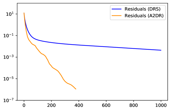
Figure 1: Nonnegative least squares: convergence of residual norms $\|r^{k}\|_{2}$.

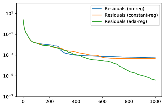
Figure 2: Nonnegative least squares: A$2$DR with no, constant, and adaptive regularization.

7.2 Sparse inverse covariance estimation

Suppose that $z_{1},\dots,z_{p}$ are i.i.d. $N(0,\Sigma)$ with $\Sigma^{-1}$ known to be sparse. We can estimate the covariance matrix $\Sigma\in{\mbox{\bf S}}_{+}^{q}$ by solving the optimization problem [19, 8]

(25) $$\begin{array}[]{ll}\mbox{minimize}&-\log\det(S)+\mbox{tr}(SQ)+\alpha\|S\|_{1},\end{array}$$

where $S\in{\mbox{\bf S}}^{q}$ (the set of symmetric matrices) is the variable, $Q=\frac{1}{p}\sum_{l=1}^{p}z_{l}z_{l}^{T}$ is the sample covariance, and $\alpha>0$ is a hyperparameter. We then take $\hat{\Sigma}=S^{-1}$ as an estimate of $\Sigma$. Here $\|S\|_{1}$ is the elementwise $\ell_{1}$ norm and $\log\det$ is understood to be an extended real-valued function, i.e., $\log\det(S)=-\infty$ whenever $S\nsucc 0$.

Let $x_{i}\in{\mbox{\bf R}}^{q(q+1)/2}$ be some vectorization of $S_{i}\in{\mbox{\bf S}}^{q}$ for $i=1,2$. Problem (25) can be represented in standard form (2) by setting

$$f_{1}(x_{1})=-\log\det(S_{1})+\mbox{tr}(S_{1}Q),\quad f_{2}(x_{2})=\alpha\|S_{2}\|_{1},$$

and $A_{1}=I$, $A_{2}=-I$, and $b=0$.

The proximal operator of $f_{1}$ can be computed by combining the affine addition rule in [39, section 2.2] with [39, section 6.7.5], while the proximal operator of $f_{2}$ is simply the shrinkage operator [39, section 6.5.2]. The overall computational cost is dominated by the eigenvalue decomposition involved in evaluating ${\mathop{\textbf{prox}}}_{tf_{1}}$, which has complexity $O(q^{3})$.

Problem instance

We generated $S\in{\mbox{\bf S}}_{++}^{q}$, the set of symmetric positive definite matrices, with $q=100$ and approximately $10\%$ nonzero entries. Then we calculated $Q$ using $p=1000$ i.i.d. samples from $\mathcal{N}(0,S^{-1})$. Let $\alpha_{\max}=\sup_{i\neq j}|Q_{ij}|$ be the smallest $\alpha$ for which the solution of (25) is trivially the diagonal matrix $(\textbf{diag}(Q)+\alpha I)^{-1}$ [8]. We solved (25) using $\alpha=0.001\alpha_{\max}$, which produced an estimate of $S$ with $7\%$ nonzero entries.

Figure 3 depicts the residual norm curves. A2DR achieves $\|r^{k}\|_{2}\leq 10^{-6}$ in less than 400 iterations, while DRS fails to fall below $10^{-4}$ even at 1000 iterations. The fluctuations in the A2DR residuals may be smoothed out by increasing the adaptive regularization coefficient $\eta$, but this generally leads to slower convergence.

We also ran A2DR on instances with $q=1200$ and $q=2000$ (vectorizations on the order of $10^{6}$) and compared its performance to SCS. In the former case, A2DR took 1 hour to converge to a tolerance of $10^{-3}$, while SCS took 11 hours to achieve a tolerance of $10^{-1}$ and yielded a much worse objective value. In the latter case, A2DR converged in 2.6 hours to a tolerance of $10^{-3}$, while SCS failed immediately with an out-of-memory error.

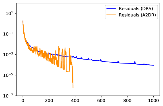
Figure 3: Sparse inverse covariance estimation: convergence of residual norms $\|r^{k}\|_{2}$.

7.3 $\ell_{1}$ trend filtering

The $\ell_{1}$ trend filtering problem is [23]

(26) $$\begin{array}[]{ll}\mbox{minimize}&\frac{1}{2}\|y-z\|_{2}^{2}+\alpha\|Dz\|_{1},\end{array}$$

where $z\in{\mbox{\bf R}}^{q}$ is the variable, $y\in{\mbox{\bf R}}^{q}$ is the problem data (e.g., time series), $\alpha\geq 0$ is a smoothing parameter, and $D\in{\mbox{\bf R}}^{(q-2)\times q}$ is the second difference operator

$$D=\left[\begin{array}[]{ccccccc}1&-2&1&0&\ldots&0&0\\ 0&1&-2&1&\ldots&0&0\\ \vdots&\vdots&\ddots&\ddots&\ddots&\vdots&\vdots\\ 0&0&\ldots&1&-2&1&0\\ 0&0&\ldots&0&1&-2&1\end{array}\right].$$

Again, we can rewrite the above problem in standard form (2) by letting

$$f_{1}(x_{1})=\frac{1}{2}\|y-x_{1}\|_{2}^{2},\quad f_{2}(x_{2})=\alpha\|x_{2}\|_{1}$$

with variables $x_{1}\in{\mbox{\bf R}}^{q},x_{2}\in{\mbox{\bf R}}^{q-2}$ and constraint matrices $A_{1}=D,A_{2}=-I$, and $b=0$. The proximal operator of $f_{1}$ is simply $\mbox{\bf prox}_{tf_{1}}(v)=\frac{ty+v}{t+1}$, and the proximal operator of $f_{2}$ is the shrinkage operator [39, section 6.5.2]. Since $D$ is tridiagonal, the projection $\Pi(v^{k+1/2})$ can be computed in $O(q)$.

Problem instance

We drew $y$ from $\mathcal{N}(0,I)$ with $q=10^{6}$ and solved (26) using $\alpha=0.01\alpha_{\max}$, where $\alpha_{\max}=\|y\|_{\infty}$ is the smallest $\alpha$ for which the solution is trivially zero.

The results are shown in Figure 4. A2DR converges about three times faster than DRS, reaching a tolerance of $10^{-6}$ in 360 iterations.

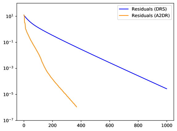
Figure 4: $\ell_{1}$ trend filtering: convergence of residual norms $\|r^{k}\|_{2}$.

7.4 Single commodity flow optimization

Consider a network with $p$ nodes and $q$ (directed) arcs described by an incidence matrix $B\in{\mbox{\bf R}}^{p\times q}$ with

$$B_{ij}=\left\{\begin{array}[]{rl}1&\mbox{arc $j$ enters node $i$},\\ -1&\mbox{arc $j$ leaves node $i$},\\ 0&\mbox{otherwise}.\end{array}\right.$$

Suppose a single commodity flows in this network. Let $z\in{\mbox{\bf R}}^{q}$ denote the arc flows and $s\in{\mbox{\bf R}}^{p}$ the node sources. We have the flow conservation constraint $Bz+s=0$. This in turn implies $\mathbf{1}^{T}s=0$ since $B^{T}\mathbf{1}=0$ by construction. The total cost of traffic on the network is the sum of a flow cost, represented by $\psi:{\mbox{\bf R}}^{q}\rightarrow{\mbox{\bf R}}\cup\{\infty\}$, and a source cost, represented by $\phi:{\mbox{\bf R}}^{p}\rightarrow{\mbox{\bf R}}\cup\{\infty\}$. We assume that these costs are separable with respect to the flows and sources, i.e., $\psi(z)=\sum_{j=1}^{q}\psi_{j}(z_{j})$ and $\phi(s)=\sum_{i=1}^{p}\phi_{i}(s_{i})$. Our goal is to choose flow and source vectors such that the network cost is minimized:

(27) $$\begin{array}[]{ll}\mbox{minimize}&\psi(z)+\phi(s)\\ \mbox{subject to}&Bz+s=0\end{array}$$

with respect to $z$ and $s$.

We consider a special case modeled on the DC power flow problem in power engineering [32]. The flow costs are quadratic with a capacity constraint:

$$\psi_{j}(z_{j})=\begin{cases}c_{j}z_{j}^{2},&|z_{j}|\leq z_{j}^{\max},\\ +\infty&\mbox{otherwise.}\end{cases}$$

The source costs are determined by the node type, which can fall into one of three categories:

1. Transfer/way-point nodes fixed at $s_{i}=0$, i.e., $\phi_{i}(s_{i})=\mathcal{I}_{\{0\}}(s_{i})$.

2. Sink nodes fixed at $s_{i}=L_{i}$ (for $L_{i}<0$), i.e., $\phi_{i}(s_{i})=\mathcal{I}_{\{L_{i}\}}(s_{i})$.

3. Source nodes with cost

   $$\phi_{i}(s_{i})=\begin{cases}d_{i}s_{i}^{2},&0\leq s_{i}\leq s_{i}^{\max},\\ +\infty&\mbox{otherwise}.\end{cases}$$

The vectors $c\in{\mbox{\bf R}}_{+}^{q},d\in{\mbox{\bf R}}_{+}^{p},z^{\max}\in{\mbox{\bf R}}^{q}$, and $s^{\max}\in{\mbox{\bf R}}^{p}$ are constants.

This problem may be restated as (2) with $x_{1}\in{\mbox{\bf R}}^{q},x_{2}\in{\mbox{\bf R}}^{p},f_{1}(x_{1})=\psi(x_{1}),\break f_{2}(x_{2})=\phi(x_{2}),A_{1}=B,A_{2}=I$, and $b=0$. Since costs are separable, the proximal operators can be calculated elementwise as

(28) $$\begin{split}(\mbox{\bf prox}_{tf_{1}}(v))_{j}&=\Pi_{[-z_{j}^{\max},z_{j}^{\max}]}\left(\frac{v_{j}}{2tc_{j}+1}\right),\quad j=1,\ldots,q,\\ (\mbox{\bf prox}_{tf_{2}}(w))_{i}&=\Pi_{[0,s_{i}^{\max}]}\left(\frac{w_{i}}{2td_{i}+1}\right),\quad i\mbox{ is a source node.}\end{split}$$

Here $\Pi_{\mathcal{C}}$ denotes the projection onto the set $\mathcal{C}$. Notice that in evaluating the proximal operator, we implicitly solve a linear system related to $L=BB^{T}$, which is the Laplacian associated with the network.

Problem instance

We set $p=4000$ and $q=7000$ and generated the incidence matrix as follows. Let $\tilde{B}\in{\mbox{\bf R}}^{p\times(q-p+1)}$, where each column $j$ is zero except for two entries $\tilde{B}_{ij}=1$ and $\tilde{B}_{i^{\prime}j}=-1$, whose positions are chosen uniformly at random. Define $\hat{B}\in{\mbox{\bf R}}^{p\times(p-1)}$ with $\hat{B}_{ii}=1$ and $\hat{B}_{(i+1)i}=-1$ for $i=1,\dots,p-1$. The final incidence matrix is $B=[\tilde{B}~{}\hat{B}]$.

To construct the source vector, we first drew $\breve{s}\in{\mbox{\bf R}}^{p}$ i.i.d. from $\mathcal{N}(0,I)$ and defined

$$\tilde{s}_{i}=\begin{cases}0,&i=1,\ldots,\lfloor\frac{p}{3}\rfloor,\\ -|\breve{s}_{i}|,&i=\lfloor\frac{p}{3}\rfloor+1,\dots,\lfloor\frac{2p}{3}\rfloor,\\ \sum_{l=\lfloor p/3\rfloor+1}^{\lfloor 2p/3\rfloor}|\breve{s}_{l}|/(p-\lfloor\frac{2p}{3}\rfloor),&i=\lfloor\frac{2p}{3}\rfloor+1,\dots,p.\end{cases}$$

We took the first $\lfloor\frac{p}{3}\rfloor$ entries to be the transfer nodes, the second $\lfloor\frac{2p}{3}\rfloor-\lfloor\frac{p}{3}\rfloor$ entries to be the sink nodes with $L_{i}=\tilde{s}_{i}$, and the last $p-\lfloor\frac{2p}{3}\rfloor$ entries to be the source nodes, where

$$s_{i}^{\max}=\begin{cases}\tilde{s}_{i}+0.001,&i=\lfloor\frac{2p}{3}\rfloor,\dots,\lfloor\frac{5p}{6}\rfloor,\\ 2(\tilde{s}_{i}+0.001),&i=\lfloor\frac{5p}{6}\rfloor,\dots,p.\end{cases}$$

To get the flow bounds, we solved $B\tilde{x}=-\tilde{s}$ for $\tilde{x}$, and let

$$x_{j}^{\max}=\begin{cases}|\tilde{x}_{j}|+0.001,&j=1,\dots,\lfloor\frac{q}{2}\rfloor,\\ 2(|\tilde{x}_{j}|+0.001),&j=\lfloor\frac{q}{2}\rfloor+1,\dots,q.\end{cases}$$

Finally, the entries of $c$ and $d$ were drawn i.i.d. from $\mbox{Uniform}(0,1)$.

Figure 5 depicts the results of our experiment. A2DR converges to a tolerance of $10^{-6}$ in less than 1200 iterations, while DRS remains above $10^{-4}$ even once the maximum iterations of 2000 is reached. For this problem, we also attempted to find a solution using SCS, but the solver failed to converge to its default tolerance of $10^{-5}$ in 5000 iterations, finishing with a linear constraint violation of $\|Bz+s\|_{2}>0.3$. In contrast, A2DR’s final result yields $\|Bz+s\|_{2}\approx 10^{-6}$.

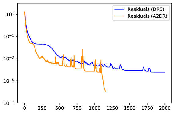
Figure 5: Single commodity flow: convergence of residual norms $\|r^{k}\|_{2}$.

7.5 Optimal control

We are interested in the following finite-horizon optimal control problem:

(29) $$\begin{array}[]{ll}\mbox{minimize}&\sum_{l=1}^{L}\phi_{l}(z_{l},u_{l})\\ \mbox{subject to}&z_{l+1}=F_{l}z_{l}+G_{l}u_{l}+h_{l},\quad l=1,\ldots,L-1,\\ &z_{1}=z_{\text{init}},\quad z_{L}=z_{\text{term}}\end{array}$$

with state variables $z_{l}\in{\mbox{\bf R}}^{q}$, control variables $u_{l}\in{\mbox{\bf R}}^{p}$, and cost functions $\phi_{l}:{\mbox{\bf R}}^{q}\times{\mbox{\bf R}}^{p}\rightarrow{\mbox{\bf R}}\cup\{\infty\}$. The data consist of an initial state $z_{\text{init}}\in{\mbox{\bf R}}^{q}$, a terminal state $z_{\text{term}}\in{\mbox{\bf R}}^{q}$, and dynamics matrices $F_{l}\in{\mbox{\bf R}}^{q\times q},G_{l}\in{\mbox{\bf R}}^{q\times p}$, and $h_{l}\in{\mbox{\bf R}}^{q}$ for $l=1,\ldots,L-1$. Let $z=(z_{1},\ldots,z_{L})\in{\mbox{\bf R}}^{Lq}$ and $u=(u_{1},\ldots,u_{L})\in{\mbox{\bf R}}^{Lp}$. If we define

$$\tilde{F}=\left[\begin{array}[]{ccccc}I&0&\ldots&0&0\\ -F_{1}&I&\ldots&0&0\\ 0&-F_{2}&\ldots&0&0\\ \vdots&\vdots&\ddots&\vdots&\vdots\\ 0&0&\ldots&-F_{L-1}&I\\ 0&0&\ldots&0&I\end{array}\right],\quad\tilde{G}=\left[\begin{array}[]{ccccc}0&0&\ldots&0&0\\ -G_{1}&0&\ldots&0&0\\ 0&-G_{2}&\ldots&0&0\\ \vdots&\vdots&\ddots&\vdots&\vdots\\ 0&0&\ldots&-G_{L-1}&0\\ 0&0&\ldots&0&0\end{array}\right],$$

and $\tilde{h}=(z_{\text{init}},h_{1},\ldots,h_{L-1},z_{\text{term}})$, then the constraints can be written compactly as $\tilde{F}z+\tilde{G}u=\tilde{h}$.

We focus on a time-invariant linear quadratic version of (29) with $F_{l}=F,G_{l}=G,h_{l}=0$, and

$$\phi_{l}(z_{l},u_{l})=\|z_{l}\|_{2}^{2}+\|u_{l}\|_{2}^{2}+\mathcal{I}_{\{u\,:\,\|u\|_{\infty}\leq 1\}}(u_{l}),\quad l=1,\ldots,L.$$

This problem is equivalent to (2) with $x_{1}\in{\mbox{\bf R}}^{Lq},x_{2}\in{\mbox{\bf R}}^{Lp}$,

$$f_{1}(x_{1})=\|x_{1}\|_{2}^{2},\quad f_{2}(x_{2})=\|x_{2}\|_{2}^{2}+\mathcal{I}_{\{u\,:\,\|u\|_{\infty}\leq 1\}}(x_{2}),$$

and constraint matrices $A_{1}=\tilde{F},A_{2}=\tilde{G}$, and $b=\tilde{h}$. The proximal operators of $f_{i}$ have closed forms $\mbox{\bf prox}_{tf_{1}}(v)=\frac{v}{2t+1}$ and $\mbox{\bf prox}_{tf_{2}}(w)=\Pi_{[-1,1]}\big{(}\frac{w}{2t+1}\big{)}$.

Problem instance

We set $p=80,q=150$, and $L=20$ and drew the entries of $F,G,h$, and $z_{\rm init}$ i.i.d. from $\mathcal{N}(0,1)$. The matrix $F$ was scaled by its spectral radius so its largest eigenvalue has magnitude one. To determine $z_{\rm term}$, we drew $\hat{u}_{l}\in{\mbox{\bf R}}^{p}$ i.i.d. from $\mathcal{N}(0,I)$, normalized to get $\tilde{u}_{l}=\hat{u}_{l}/\|\hat{u}_{l}\|_{\infty}$, and computed $\tilde{z}_{l+1}=F\tilde{z}_{l}+G\tilde{u}_{l}+h$ for $l=1,\ldots,L-1$ starting from $\tilde{z}_{1}=z_{\rm init}$. We then chose the terminal state to be $z_{\rm term}=\tilde{z}_{L}$.

Figure 6 depicts the residual curves for problem (29). DRS requires over five times as many iterations to converge as A2DR, which reaches a tolerance of $10^{-6}$ in just under 100 iterations. For comparison, we solved the same problem in CVXPY with OSQP and SCS and found that neither solver converged to its default tolerance ($10^{-4}$ and $10^{-5}$, respectively) by its maximum number of iterations. Indeed, OSQP returned a solver error, while SCS terminated with a linear constraint violation of $\|\tilde{F}z+\tilde{G}u-\tilde{h}\|_{2}>0.9$. A2DR’s final constraint violation is only about $10^{-6}$.

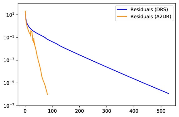
Figure 6: Optimal control: convergence of residual norms $\|r^{k}\|_{2}$.

7.6 Coupled quadratic program

We consider a quadratic program in which $L$ variable blocks are coupled through a set of $s$ linear constraints, represented as

(30) $$\begin{array}[]{ll}\mbox{minimize}&\sum_{l=1}^{L}z_{l}^{T}Q_{l}z_{l}+c_{l}^{T}z_{l}\\ \mbox{subject to}&F_{l}z_{l}\leq d_{l},\quad l=1,\dots,L,\\ &\sum_{l=1}^{L}G_{l}z_{l}=h\end{array}$$

with respect to $z=(z_{1},\dots,z_{L})$, where $z_{l}\in{\mbox{\bf R}}^{q_{l}},Q_{l}\in{\mbox{\bf S}}_{+}^{q_{l}},c_{l}\in{\mbox{\bf R}}^{q_{l}},F_{l}\in{\mbox{\bf R}}^{p_{l}\times q_{l}},d_{l}\in{\mbox{\bf R}}^{p_{l}},G_{l}\in{\mbox{\bf R}}^{s\times q_{l}}$, and $h\in{\mbox{\bf R}}^{s}$ for $l=1,\ldots,L$.

We can rewrite (30) in standard form with $N=L$, $x=z$,

$$f_{i}(x_{i})=x_{i}^{T}Q_{i}x_{i}+c_{i}^{T}x_{i}+\mathcal{I}_{\{x\,:\,F_{i}x\leq d_{i}\}}(x_{i}),\quad i=1,\ldots,L,$$

$A=[G_{1}~{}\cdots~{}G_{L}]$, and $b=h$. The proximal operator ${\mathop{\textbf{prox}}}_{tf_{i}}(v_{i})$ is evaluated by solving

(31) $$\begin{array}[]{ll}\mbox{minimize}&x_{i}^{T}\left(Q_{i}+\frac{1}{2t}I\right)x_{i}+(c_{i}-\frac{1}{t}v_{i})^{T}x_{i}\\ \mbox{subject to}&F_{i}x_{i}\leq d_{i}\\ \end{array}$$

with respect to $x_{i}\in{\mbox{\bf R}}^{q_{i}}$.

Problem instance

Let $L=8$, $s=50$, $q_{l}=300$, and $p_{l}=200$ for $l=1,\ldots,L$. We generated the entries of $c_{l}\in{\mbox{\bf R}}^{q_{l}},F_{l}\in{\mbox{\bf R}}^{p_{l}\times q_{l}},G_{l}\in{\mbox{\bf R}}^{s\times q_{l}},\tilde{z}_{l}\in{\mbox{\bf R}}^{q_{l}}$, and $H_{l}\in{\mbox{\bf R}}^{q_{l}\times q_{l}}$ i.i.d. from $\mathcal{N}(0,1)$. We then formed $d_{l}=F_{l}\tilde{z}_{l}+0.1,Q_{l}=H_{l}^{T}H_{l}$, and $h=\sum_{l=1}^{L}G_{l}\tilde{z}_{l}$. To evaluate the proximal operators, we constructed problem (31) in CVXPY and solved it using OSQP with the default tolerance.

The results of our experiment are shown in Figure 7. A2DR produces an over ten-fold speedup, converging to the desired tolerance of $10^{-6}$ in only $60$ iterations.

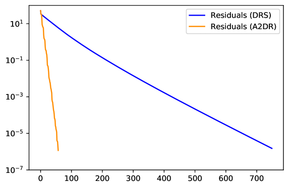
Figure 7: Coupled quadratic program: convergence of residual norms $\|r^{k}\|_{2}$.

7.7 Multitask regularized logistic regression

Consider the following multi-task regression problem:

(32) $$\begin{array}[]{ll}\mbox{minimize}&\phi(W\theta,Y)+r(\theta)\end{array}$$

with variable $\theta=[\theta_{1}\cdots\theta_{L}]\in{\mbox{\bf R}}^{s\times L}$. Here $\phi:{\mbox{\bf R}}^{p\times L}\times{\mbox{\bf R}}^{p\times L}\rightarrow{\mbox{\bf R}}$ is the loss function, $r:{\mbox{\bf R}}^{s\times L}\rightarrow{\mbox{\bf R}}$ is the regularizer, $W\in{\mbox{\bf R}}^{p\times s}$ is the feature matrix shared across the $L$ tasks, and $Y=[y_{1}\cdots y_{L}]\in{\mbox{\bf R}}^{p\times L}$ contains the $p$ class labels for each task $l=1,\ldots,L$.

We focus on the binary classification problem, so that all entries of $Y$ are $\pm 1$. Accordingly, we take our loss function to be the logistic loss summed over samples and tasks,

$$\phi(Z,Y)=\sum_{l=1}^{L}\sum_{i=1}^{p}\log\left(1+\exp(-Y_{il}Z_{il})\right),$$

where $Z\in{\mbox{\bf R}}^{p\times L}$, and our regularizer to be a linear combination of the group lasso penalty [20] and the nuclear norm,

$$r(\theta)=\alpha\|\theta\|_{2,1}+\beta\|\theta\|_{*},$$

where $\|\theta\|_{2,1}=\sum_{l=1}^{L}\|\theta_{l}\|_{2}$ and $\alpha>0,~{}\beta>0$ are regularization parameters.

Problem (32) can be converted to standard form (2) by letting

$$f_{1}(Z)=\phi(Z,Y),\quad f_{2}(\theta)=\alpha\|\theta\|_{2,1},\quad f_{3}(\tilde{\theta})=\beta\|\tilde{\theta}\|_{*},$$

$$A=\left[\begin{array}[]{cccc}I&-W&0\\ 0&I&-I\end{array}\right],\quad x=\left[\begin{array}[]{c}Z\\ \theta\\ \tilde{\theta}\end{array}\right],\quad b=0.$$

The proximal operator of $f_{1}$ can be evaluated efficiently via Newton type methods applied to each component in parallel [14], while the proximal operators of the regularization terms have closed-form expressions [39, sections 6.5.4 and 6.7.3].

Problem instance

We let $p=300$, $s=500$, $L=10$, and $\alpha=\beta=0.1$. The entries of $W\in{\mbox{\bf R}}^{p\times s}$ and $\theta^{\star}\in{\mbox{\bf R}}^{s\times L}$ were drawn i.i.d. from $\mathcal{N}(0,1)$. We calculated $Y=\textbf{sign}(W\theta^{\star})$, where the signum function is applied elementwise with the convention $\textbf{sign}(0)=-1$. To evaluate ${\mathop{\textbf{prox}}}_{tf_{1}}$, we used the Newton-CG method from scipy.optimize.minimize, warm starting each iteration with the output from the previous iteration. (Further performance improvements may be achieved by implementing Newton’s method with unit step size and initial point zero for each component in parallel [14].)

Figure 8 shows the residual plots for A2DR and DRS. The A2DR curve exhibits a steep drop in the first few steps and continues falling until convergence at 500 iterations. In contrast, the DRS residual norms never make it below a tolerance of $10^{-2}$.

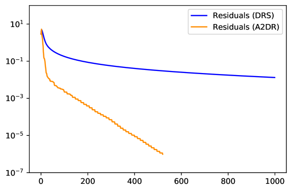
Figure 8: Multitask regularized logistic regression: convergence of residual norms $\|r^{k}\|_{2}$.

8 Conclusions

We have presented an algorithm for solving linearly constrained convex optimization problems, where the objective function is only accessible via its proximal operator. Our algorithm is an application of type-II Anderson acceleration to Douglas–Rachford splitting (A2DR). Under relatively mild conditions, we prove that A2DR either converges to a global optimum or provides a certificate of infeasibility/unboundedness. Moreover, when the objective is block separable, its steps partially decouple so that they may be computed in parallel, enabling fast distributed implementations. We provide one such Python implementation at https://github.com/cvxgrp/a2dr. Using only the default parameters, we show that our solver achieves rapid convergence on a wide range of problems, making it a robust choice for general large-scale convex optimization.

In the future, we plan to release a user-friendly interface, which automatically reduces a problem to the standard form (2) input of the A2DR solver, similar to the Epsilon system [58]. This will allow us to integrate A2DR into a high-level domain specific language for convex optimization. We also intend to expand the library of proximal operators. As problems grow larger, we aim to support more parallel computing architectures, allowing users to leverage GPU acceleration and high-performance clusters for distributed optimization.

In this supplementary material, we provide the proofs for the theorems in the main text.

Appendix A Preliminaries

We begin with the following lemma, which establishes the connection between residuals of the DRS fixed-point mapping and the primal/dual residuals of the original problem (2).

Lemma A.1.

Suppose that $\liminf_{j\rightarrow\infty}\|v^{j}-F_{\rm DRS}(v^{j})\|_{2}\leq\epsilon$ for some $\epsilon\geq 0$. Then

(33) $$\liminf_{j\rightarrow\infty}\|r_{\rm prim}^{j}\|_{2}\leq\|A\|_{2}\epsilon,\quad\liminf_{j\rightarrow\infty}\|r_{\rm dual}^{j}\|_{2}\leq\frac{1}{t}\epsilon.$$

Proof A.2.

By expanding $F_{\rm DRS}$, and in particular line 6 of Algorithm 1, we see that

$$\liminf_{j\rightarrow\infty}\|x^{j+1/2}-x^{j+1}\|_{2}=\liminf_{j\rightarrow\infty}\|v^{j}-v_{\rm DRS}^{j+1}\|_{2}\leq\epsilon.$$

Since $Ax^{j+1}=b$ by the projection step in $F_{\rm DRS}$, we have

$$r_{\rm prim}^{j}=Ax^{j+1/2}-b=A(x^{j+1/2}-x^{j+1}),$$

which implies that

$$\liminf_{j\rightarrow\infty}\|r_{\rm prim}^{j}\|_{2}\leq\|A\|_{2}\liminf_{j\rightarrow\infty}\|x^{j+1/2}-x^{j+1}\|_{2}\leq\|A\|_{2}\epsilon,$$

and hence $\liminf_{j\rightarrow\infty}\|r_{\rm prim}^{j}\|_{2}\leq\|A\|_{2}\epsilon$.

On the other hand, the optimality conditions from lines 3 and 5 of Algorithm 1 give us

$$\frac{1}{t}(x^{j+1/2}-v^{j})+g^{j}=0,\quad x^{j+1}=v^{j+1/2}-A^{T}\tilde{\lambda}^{j},$$

for some $g^{j}\in\partial f(x^{j+1/2})$ and $\tilde{\lambda}^{j}=(AA^{T})^{\dagger}(Av^{j+1/2}-b)$. Thus,

(34) $$\begin{split}g^{j}&=\frac{1}{t}(v^{j}-x^{j+1/2})\\ &=\frac{1}{t}(v^{j+1/2}-x^{j+1})+\frac{1}{t}(v^{j}-v^{j+1/2})+\frac{1}{t}(x^{j+1}-x^{j+1/2})\\ &=\frac{1}{t}A^{T}\tilde{\lambda}^{j}+2\frac{1}{t}(v^{j}-x^{j+1/2})+\frac{1}{t}(x^{j+1}-x^{j+1/2})\\ &=\frac{1}{t}A^{T}\tilde{\lambda}^{j}+2g^{j}+\frac{1}{t}(x^{j+1}-x^{j+1/2}),\end{split}$$

where we have used line 4 of Algorithm 1 in the third equality. Rearranging terms yields $g^{j}=A^{T}(-\frac{1}{t}\tilde{\lambda}^{j})+\frac{1}{t}(x^{j+1/2}-x^{j+1})$.

Finally, since we compute $r_{\rm dual}^{j}=g^{j}+A^{T}\lambda^{j}$ using $\lambda^{j}\in\mathop{\rm argmin}_{\lambda}\|g^{j}+A^{T}\lambda\|_{2}$ (c.f. residuals and dual variables in §2),

$$\liminf_{j\rightarrow\infty}\|r_{\rm dual}^{j}\|_{2}\leq\liminf_{j\rightarrow\infty}\|g^{j}+A^{T}\bar{\lambda}^{j}\|_{2}=\frac{1}{t}\liminf_{j\rightarrow\infty}\|x^{j+1/2}-x^{j+1}\|_{2}\leq\frac{1}{t}\epsilon,$$

where $\bar{\lambda}^{j}=\frac{1}{t}\tilde{\lambda}^{j}$. This completes our proof.

Remark A.3.

When $\epsilon=0$, Lemma A.1 implies that

$$\liminf_{j\rightarrow\infty}\|r_{\rm prim}^{j}\|_{2}=\liminf_{j\rightarrow\infty}\|r_{\rm dual}^{j}\|_{2}=0.$$

Furthermore, notice that we could have calculated $r_{\rm dual}^{j}$ using

$$\lambda^{j}=\bar{\lambda}^{j}=\frac{1}{t}(AA^{T})^{\dagger}(Av^{k+1/2}-b),$$

and the results would still hold.

Appendix B Proof of Theorems 4.5 and 4.7

We now prove the convergence results in the error-free setting. Define the infimal displacement vector of $F_{\rm DRS}$ as $\delta v^{\star}=\Pi_{\overline{\mathop{\bf range}(I-F_{\rm DRS})}}(0)$. It follows directly that $\|\delta v^{\star}\|_{2}=\inf_{v\in\mathbf{R}^{n}}~{}\|v-F_{\rm DRS}(v)\|_{2}$. We will later show that in A2DR, $\lim_{k\rightarrow\infty}v^{k}-v^{k+1}=\delta v^{\star}$. In particular, Theorem 4.7 gives us $\delta v=\delta v^{\star}$.

We begin by showing that $\delta v^{\star}=0$ if and only if problem (2) is solvable. To see this, first notice that by [65, Corollary 6.5],

$$\delta v^{\star}=\mathop{\rm argmin}\nolimits_{z\in\mathcal{Z}}\|z\|_{2},$$

where

$$\mathcal{Z}=\overline{\mathop{\bf dom}f-\mathop{\bf dom}g}\cap t(\overline{\mathop{\bf dom}f^{*}+\mathop{\bf dom}g^{*}}),\quad g(x)=\mathcal{I}_{\{v\,:\,Av=b\}}(x).$$

Since $\mathop{\bf dom}g=\{x\,:\,Ax=b\}$ and $\mathop{\bf dom}g^{*}=\mathop{\bf range}(A^{T})=-\mathop{\bf range}(A^{T})$, the problem is solvable if and only if

$$\mathop{\bf dist{}}(\mathop{\bf dom}f,\mathop{\bf dom}g)=\mathop{\bf dist{}}(\mathop{\bf dom}f^{*},-\mathop{\bf dom}g^{*})=0,$$

which holds if and only if $0\in\overline{\mathop{\bf dom}f-\mathop{\bf dom}g}$ and $0\in\overline{\mathop{\bf dom}f^{*}+\mathop{\bf dom}g^{*}}$, i.e., $\delta v^{\star}=0$.

Below we denote the initial iteration counts for accepting AA candidates as $k_{i}$ (i.e., when $I_{\rm safeguard}$ is True or $R_{\rm AA}\geq R$, and the check in Algorithm 2, line 14 passes), and the iteration counts for accepting DRS candidates as $l_{i}$. Notice that for each iteration $k$, either $k=k_{i}+K$ for some $i$ and $0\leq K\leq R-1$, or $k=l_{i}$ for some $i$.

• Case (i) [Theorem 4.5, (18)]

  First, suppose that problem (2) is solvable. Then, $\delta v^{\star}=0$. By Lemma A.1, to prove (18), it suffices to prove that $\liminf_{k\rightarrow\infty}\|g^{k}\|_{2}=0$. If the set of $k_{i}$ is infinite, i.e., the AA candidate is adopted an infinite number of times, then

  $$0\leq\liminf_{k\rightarrow\infty}\|g^{k}\|_{2}\leq\liminf_{i\rightarrow\infty}\|g^{k_{i}}\|_{2}\leq D\|g^{0}\|_{2}\lim_{i\rightarrow\infty}(i+1)^{-(1+\epsilon)}=0.$$

  Here we used the fact that $n_{AA}/R=i$ in iteration $k_{i}$.

  On the other hand, if the set of $k_{i}$ is finite, Algorithm 2 reduces to the vanilla DRS algorithm after a finite number of iterations. By [67, Theorem 2], this means that $\lim_{k\rightarrow\infty}g^{k}=\lim_{k\rightarrow\infty}v^{k}-v^{k+1}=\delta v^{\star}=0$. Thus, we always have $\liminf_{k\rightarrow\infty}\|g^{k}\|_{2}=0$, and this fact coupled with Lemma A.1 immediately gives us (18).

  Notice that the case of finite $k_{i}$’s cannot actually happen. Otherwise, since $\lim_{k\rightarrow\infty}\|g^{k}\|_{2}=0$ and $n_{AA}$ is upper bounded (because AA candidates are rejected after some point), the check on line 14 of Algorithm 2 must pass eventually. This means that an AA candidate is accepted one more time, which is a contradiction. Hence it must be that AA candidates are adopted an infinite number of times.

• Case (ii) [Theorem 4.5, iteration convergence]

  Now suppose that $F_{\rm DRS}$ has a fixed point. As $G_{\rm DRS}$ is non-expansive, if the AA candidate is adopted in iteration $k$,

  $$\begin{split}\|g^{k+1}\|_{2}&=\|G_{\rm DRS}(v^{k+1})\|_{2}\leq\|G_{\rm DRS}(v^{k+1})-G_{\rm DRS}(v^{k})\|_{2}+\|G_{\rm DRS}(v^{k})\|_{2}\\ &\leq(\|H_{k}\|_{2}+1)\|g^{k}\|_{2}\leq 2(1+1/\eta)\|g^{k}\|_{2},\end{split}$$

  where we have used Lemma 4.3 to bound $\|H_{k}\|_{2}$. This immediately implies that for any $0\leq K\leq R-1$,

  (35) $$\|g^{k_{i}+K}\|_{2}\leq(2+2/\eta)^{K}\|g^{k_{i}}\|_{2}\leq D\|g^{0}\|_{2}(2+2/\eta)^{K}(i+1)^{-(1+\epsilon)},$$

  and so we have $\lim_{i\rightarrow\infty}\|g^{k_{i}+K}\|_{2}=0$.

  In addition, since AA candidates are accepted in all iterations $k_{i}+K$, again by Lemma 4.3, we have that for any $w\in{\mbox{\bf R}}^{n}$,

  (36) $$\begin{split}\|v^{k_{i}+K+1}-w\|_{2}&\leq\|v^{k_{i}+K}-w\|_{2}+(1+2/\eta)\|g^{k_{i}+K}\|_{2}\\ &\leq\cdots\leq\|v^{k_{i}}-w\|_{2}+(1+2/\eta)\sum_{j=0}^{K}\|g^{k_{i}+j}\|_{2}\\ &\leq\|v^{k_{i}}-w\|_{2}+(1+2/\eta)\|g^{k_{i}}\|_{2}\sum_{j=0}^{K}(2+2/\eta)^{j}\\ &\leq\|v^{k_{i}}-w\|_{2}+(1+2/\eta)C_{R}D\|g^{0}\|_{2}(i+1)^{-(1+\epsilon)},\end{split}$$

  where $C_{R}=\sum_{j=0}^{R-1}(2+2/\eta)^{j}$ is a constant.

  Now let $v^{\star}$ be a fixed point of $F_{\rm DRS}$. Since $F_{\rm DRS}$ is $1/2$-averaged, by inequality (5) in [43],

  (37) $$\|v^{l_{i}+1}-v^{\star}\|_{2}^{2}\leq\|v^{l_{i}}-v^{\star}\|_{2}^{2}-\|g^{l_{i}}\|_{2}^{2}\leq\|v^{l_{i}}-v^{\star}\|_{2}^{2}$$

  for any $i\geq 0$. Hence for any $k\geq 0$,

  $$\|v^{k}-v^{\star}\|_{2}\leq\|v^{0}-v^{\star}\|_{2}+(1+2/\eta)C_{R}D\|g^{0}\|_{2}\sum\nolimits_{i=0}^{\infty}(i+1)^{-(1+\epsilon)}=E<\infty,$$

  implying that $\|v^{k}-v^{\star}\|_{2}$ is bounded.

  As a result, by squaring both sides of (36) and combining with (37), we get that

  $$\sum_{i=0}^{\infty}\|g^{l_{i}}\|_{2}^{2}\leq\|v^{0}-v^{\star}\|_{2}^{2}+\text{const},$$

  where

  $$\begin{split}\text{const}=&\left((1+2/\eta)C_{R}D\|g^{0}\|_{2}\right)^{2}\sum_{i=0}^{\infty}(i+1)^{-(2+2\epsilon)}\\ &+(2+4/\eta)C_{R}DE\|g^{0}\|_{2}\sum_{i=0}^{\infty}(i+1)^{-(1+\epsilon)}<\infty.\end{split}$$

  Thus, $\lim_{i\rightarrow\infty}\|g^{l_{i}}\|_{2}=0$. Together with the fact that $\lim_{i\rightarrow\infty}\|g^{k_{i}+K}\|_{2}=0$ for $0\leq K\leq R-1$, we immediately obtain $\lim_{k\rightarrow\infty}\|g^{k}\|_{2}=0$, and an application of Lemma A.1 yields (18).

  Notice that in our derivation, we implicitly assumed both index sets are infinite. The set of $k_{i}$ is always infinite by the same logic as in case (i). Moreover, if the set of $l_{i}$ is finite, the arguments above involving $l_{i}$ can be ignored, as eventually $k=k_{i}+K$ for all $i$ above some threshold.

  It still remains to be shown that $v^{k}$ converges to a fixed-point of $F_{\rm DRS}$. To do this, we first show that $\|v^{k}-v^{\star}\|_{2}$ is quasi-Fejérian. Squaring both sides of the first inequality in (36) and combining it with (35) and (37), we get that for any $k\geq 0$,

  (38) $$\|v^{k+1}-v^{\star}\|_{2}^{2}\leq\|v^{k}-v^{\star}\|_{2}^{2}+\epsilon^{k},$$

  where $\epsilon^{l_{i}}=0$ and

  $$\begin{split}\epsilon^{k_{i}+K}=&2DE\|g^{0}\|_{2}(1+2/\eta)(2+2/\eta)^{K}(i+1)^{-(1+\epsilon)}\\ &+\left(D\|g^{0}\|_{2}(1+2/\eta)\right)^{2}(2+2/\eta)^{2K}(i+1)^{-(2+2\epsilon)}\end{split}$$

  for $0\leq K\leq R-1$. Hence $\epsilon^{k}\geq 0$ and $\sum_{k=0}^{\infty}\epsilon^{k}<\infty$. In other words, $\|v^{k}-v^{\star}\|_{2}$ is quasi-Fejérian.

  Since $\lim_{k\rightarrow\infty}\|g^{k}\|_{2}=0$ and inequality (38) holds, we can invoke [66, Theorem 3.8] to conclude that $\lim_{k\rightarrow\infty}\|v^{k}-v^{\star}\|_{2}$ exists and $v^{k}$ converges to some fixed-point of $F_{\rm DRS}$ (not necessarily $v^{\star}$). The convergence of $x^{k+1/2}$ to a solution of (2) follows directly from the continuity of the proximal operators.

• Case (iii) [Theorem 4.7]

  Now suppose that problem (2) is pathological, then $\delta v^{\star}\neq 0$. Since

  $$\|\delta v^{\star}\|_{2}=\inf_{v\in\mathbf{R}^{n}}~{}\|v-F_{\rm DRS}(v)\|_{2},$$

  the safeguard will always be invoked for sufficiently large iteration $k$ because $\|g^{k}\|_{2}\geq\|\delta v^{\star}\|_{2}>0$. Hence the algorithm reduces to vanilla DRS in the end. We can thus prove the result in case (iii) by appealing to previous work on vanilla DRS [67, 65, 44].

  Recall that $\lim_{k\rightarrow\infty}v^{k}-v^{k+1}=\delta v^{\star}\neq 0$ [67, Theorem 2]. First, we will show that problem (2) is dual strongly infeasible if and only if

  $$\lim_{k\rightarrow\infty}Ax^{k+1/2}=b.$$

  If the problem is dual strongly infeasible, then by [44, Lemma 1], it is primal feasible and has an improving direction $d=-\frac{1}{t}\delta v^{\star}$ [44, Corollary 3]. Along this direction, both $f$ and $g=\mathcal{I}_{\{x\,:\,Ax=b\}}$ remain feasible, and in particular, $A\delta v^{\star}=0$. Hence

  $$\lim_{k\rightarrow\infty}Ax^{k+1/2}-Ax^{k+1}=\lim_{k\rightarrow\infty}A(v^{k}-v^{k+1})=A\delta v^{\star}=0,$$

  which implies that $\lim_{k\rightarrow\infty}Ax^{k+1/2}=b$ since $Ax^{k+1}=b$ for all $k\geq 0$.

  Conversely, if $\lim_{k\rightarrow\infty}Ax^{k+1/2}=b$, then $\mathop{\bf dist{}}(\mathop{\bf dom}f,\mathop{\bf dom}g)=0$ because $x^{k+1/2}\in\mathop{\bf dom}f$. This implies problem (2) is not primal strongly infeasible, so it must be dual strongly infeasible since we assumed the problem is pathological.

  Hence if $\lim_{k\rightarrow\infty}Ax^{k+1/2}=b$, problem (2) is dual strongly infeasible, and by [44, Lemma 1 and Corollary 3], it is unbounded and

  $$\delta v^{\star}=t\Pi_{\overline{\mathop{\bf dom}f^{*}+\mathop{\bf dom}g^{*}}}(0),$$

  which implies that

  $$\|\delta v^{\star}\|_{2}=t\mathop{\bf dist{}}(\mathop{\bf dom}f^{*},\mathop{\bf range}(A^{T})).$$

  Otherwise, the problem is not dual strongly infeasible and thus must be primal strongly infeasible by our assumption of pathology, so from [65, Corollary 6.5],

  $$\|\delta v\|_{2}\geq\mathop{\bf dist{}}(\mathop{\bf dom}f,\{x\,:\,Ax=b\}).$$

  When the dual problem is feasible, $\delta v^{\star}=\Pi_{\overline{\mathop{\bf dom}f-\mathop{\bf dom}g}}(0)$ [44, Corollary 5], which implies that

  $$\|\delta v^{\star}\|_{2}=\mathop{\bf dist{}}(\mathop{\bf dom}f,\{x\,:\,Ax=b\}).$$

Appendix C Proof of Theorem 4.6

The proof resembles that of Theorem 4.5 (with identical notation), so here we mainly highlight the differences caused by the computational errors $\eta_{1}^{k},~{}\eta_{2}^{k}$. We begin by bounding the difference between the error-corrupted fixed-point mapping, denoted by $\hat{F}_{\rm DRS}$, and the error-free mapping $F_{\rm DRS}$. Starting from any $v^{k}\in{\mbox{\bf R}}^{n}$, we have by definition

$$\|\hat{v}^{k+1/2}-v^{k+1/2}\|_{2}=2\|\hat{x}^{k+1/2}-x^{k+1/2}\|_{2}=2\|\eta_{1}^{k}\|_{2},$$

$$\|\hat{x}^{k+1}-x^{k+1}\|_{2}\leq\|\hat{v}^{k+1/2}-v^{k+1/2}\|_{2}+\|\eta_{2}^{k}\|_{2}=2\|\eta_{1}^{k}\|_{2}+\|\eta_{2}^{k}\|_{2},$$

where the inequality comes from the non-expansiveness of $\Pi$. Let $\hat{G}_{\rm DRS}(v)=v-\hat{F}_{\rm DRS}(v)$. Since $\|\eta_{1}^{k}\|_{2}\leq\epsilon^{\prime}$ and $\|\eta_{2}^{k}\|_{2}\leq\epsilon^{\prime}$,

$$\begin{split}\|g^{k}-G_{\rm DRS}(v^{k})\|_{2}&=\|\hat{G}_{\rm DRS}(v^{k})-G_{\rm DRS}(v^{k})\|_{2}\\ &=\|\hat{F}_{\rm DRS}(v^{k})-F_{\rm DRS}(v^{k})\|_{2}\\ &\leq\|\hat{x}^{k+1}-x^{k+1}\|_{2}+\|\hat{x}^{k+1/2}-x^{k+1/2}\|_{2}\\ &\leq 3\|\eta_{1}^{k}\|_{2}+\|\eta_{2}^{k}\|_{2}\leq 4\epsilon^{\prime}.\end{split}$$

Thus, by Lemma A.1, it suffices to prove that $\liminf_{k\rightarrow\infty}\|G_{\rm DRS}(v^{k})\|_{2}\leq 4\epsilon^{\prime}+4\sqrt{L\epsilon^{\prime}}$.

On the one hand, if the set of $k_{i}$ (AA candidates) is infinite,

$$\begin{split}\liminf_{k\rightarrow\infty}\|G_{\rm DRS}(v^{k})\|_{2}&\leq\liminf_{i\rightarrow\infty}\|G_{\rm DRS}(v^{k_{i}})\|_{2}\leq\liminf_{i\rightarrow\infty}\|g^{k_{i}}\|_{2}+4\epsilon^{\prime}\\ &\leq D\|g^{0}\|_{2}\lim_{i\rightarrow\infty}(i+1)^{-(1+\epsilon)}+4\epsilon^{\prime}=4\epsilon^{\prime}.\end{split}$$

Otherwise, the set of $k_{i}$ is finite, and the algorithm reduces to vanilla DRS after a finite number of iterations. Without loss of generality, suppose we start running the error-corrupted vanilla DRS algorithm from the first iteration.

Let $v^{\star}$ be a fixed-point of $F_{\rm DRS}$. By inequality (5) in [43],

(39) $$\begin{split}\|v^{k+1}-v^{\star}\|_{2}^{2}&\leq\left(\|\hat{F}_{\rm DRS}(v^{k})-F_{\rm DRS}(v^{k})\|_{2}+\|F_{\rm DRS}(v^{k})-v^{\star}\|_{2}\right)^{2}\\ &\leq 16(\epsilon^{\prime})^{2}+8\epsilon^{\prime}\|v^{k}-v^{\star}\|_{2}+\|F_{\rm DRS}(v^{k})-v^{\star}\|_{2}^{2}\\ &\leq 16(\epsilon^{\prime})^{2}+16L\epsilon^{\prime}+\|v^{k}-v^{\star}\|_{2}^{2}-\|G_{\rm DRS}(v^{k})\|_{2}^{2}\end{split}$$

for all $k\geq 0$, where in the second step, we use the fact that $\|\hat{F}_{\rm DRS}(v^{k})-F_{\rm DRS}(v^{k})\|_{2}\leq 4\epsilon^{\prime}$ and $F_{\rm DRS}$ is non-expansive, and in the third step, we employ $\|v^{k}\|_{2}\leq L$ and $\|v^{\star}\|_{2}\leq L$ along with the triangle inequality. Rearranging terms and telescoping the inequalities,

$$\dfrac{1}{K}\sum_{k=0}^{K-1}\|G_{\rm DRS}(v^{k})\|_{2}^{2}\leq\dfrac{1}{K}\|v^{0}-v^{\star}\|_{2}^{2}+16(\epsilon^{\prime})^{2}+16L\epsilon^{\prime},$$

which immediately implies that

$$\liminf_{k\rightarrow\infty}\|G_{\rm DRS}(v^{k})\|_{2}\leq\sqrt{16(\epsilon^{\prime})^{2}+16L\epsilon^{\prime}}\leq 4\epsilon^{\prime}+4\sqrt{L\epsilon^{\prime}}.$$

Together with Lemma A.1, this completes the proof.

References

- [1] M. Abramowitz and I. A. Stegun, Handbook of Mathematical Functions with Formulas, Graphs, and Mathematical Tables, U.S. National Bureau of Standards, Washington, DC, 1964.
- [2] A. Agrawal, R. Verschueren, S. Diamond, and S. Boyd, A rewriting system for convex optimization problems, J. Control Decis., 5 (2018), pp. 42–60.
- [3] A. C. Aitken, On Bernoulli’s numerical solution of algebraic equations, Proc. Roy. Soc. Edinburgh, 46 (1927), pp. 289–305.
- [4] A. Ali, E. Wong, and J. Z. Kolter, A semismooth Newton method for fast, generic convex programming, in Proceedings of the International Conference on Machine Learning, 2017, pp. 70–79.
- [5] D. G. Anderson, Iterative procedures for nonlinear integral equations, J. Assoc. Comput. Mach., 12 (1965), pp. 547–560.
- [6] N. S. Aybat, Z. Wang, T. Lin, and S. Ma, Distributed linearized alternating direction method of multipliers for composite convex consensus optimization, IEEE Trans. Automat. Control, 63 (2018), pp. 5–20.
- [7] F. Bach, Acceleration without pain, https://francisbach.com/acceleration-without-pain, Feb. 4, 2020.
- [8] O. Banerjee, L. E. Ghaoui, and A. d’Aspremont, Model selection through sparse maximum likelihood estimation for multivariate Gaussian or binary data, J. Mach. Learn. Res., 9 (2008), pp. 485–516.
- [9] P. Bansode, K. C. Kosaraju, S. R. Wagh, R. Pasumarthy, and N. M. Singh, Accelerated distributed primal-dual dynamics using adaptive synchronization, IEEE Access, 7 (2019), pp. 120424–120440.
- [10] S. Boyd, N. Parikh, E. Chu, B. Peleato, and J. Eckstein, Distributed optimization and statistical learning via the alternating direction method of multipliers, Found. Trends Mach. Learn., 3 (2011), pp. 1–122.
- [11] S. Boyd and L. Vandenberghe, Convex Optimization, Cambridge University Press, Cambridge, 2004.
- [12] C. Brezinski, M. Redivo-Zaglia, and Y. Saad, Shanks sequence transformations and Anderson acceleration, SIAM Rev., 60 (2018), pp. 646–669, https://doi.org/10.1137/17M1120725.
- [13] X. Chen and C. T. Kelley, Convergence of the EDIIS algorithm for nonlinear equations, SIAM J. Sci. Comput., 41 (2019), pp. A365–A379, https://doi.org/10.1137/18M1171084.
- [14] A. Defazio, A simple practical accelerated method for finite sums, in Proceedings of the 30th International Conference on Neural Information Processing Systems, 2016, pp. 676–684.
- [15] S. Diamond and S. Boyd, CVXPY: A Python-embedded modeling language for convex optimization, J. Mach. Learn. Res., 17 (2016), pp. 1–5.
- [16] C. Evans, S. Pollock, L. G. Rebholz, and M. Xiao, A Proof that Anderson Acceleration Increases the Convergence Rate in Linearly Converging Fixed Point Methods (But Not in Quadratically Converging Ones), preprint, https://arxiv.org/abs/1810.08455, 2018.
- [17] H. Fang and Y. Saad, Two classes of multisecant methods for nonlinear acceleration, Numer. Linear Algebra Appl., 16 (2009), pp. 197–221.
- [18] C. Fougner and S. Boyd, Parameter selection and preconditioning for a graph form solver, in Emerging Applications of Control and Systems Theory, R. Tempo, S. Yurkovich, and P. Misra, eds., Lect. Notes Control Inf. Sci. Proc., Springer, Cham, pp. 41–61.
- [19] J. Friedman, T. Hastie, and R. Tibshirani, Sparse inverse covariance estimation with the graphical lasso, Biostatistics, 9 (2008), pp. 432–441.
- [20] J. Friedman, T. Hastie, and R. Tibshirani, A Note on the Group Lasso and a Sparse Group Lasso, preprint, https://arxiv.org/abs/1001.0736, 2010.
- [21] B. S. He, H. Yang, and S. L. Wang, Alternating direction method with self-adaptive penalty parameters for monotone variational inequalities, J. Optim. Theory Appl., 106 (2000), pp. 337–356.
- [22] H. He and D. Han, A distributed Douglas-Rachford splitting method for multi-block convex minimization problems, Adv. Comput. Math., 42 (2016), pp. 27–53.
- [23] S.-J. Kim, K. Koh, S. Boyd, and D. Gorinevsky, trend filtering, SIAM Rev., 51 (2009), pp. 339–360, https://doi.org/10.1137/070690274.
- [24] K. N. Kudin and G. E. Scuseria, A black-box self-consistent field convergence algorithm: One step closer, J. Chem. Phys., 116 (2002), pp. 8255–8261.
- [25] Z. Li and J. Li, An Anderson-Chebyshev Mixing Method for Nonlinear Optimization, preprint, https://arxiv.org/abs/1809.02341, 2018.
- [26] Y. Liu, E. K. Ryu, and W. Yin, A new use of Douglas-Rachford splitting for identifying infeasible, unbounded, and pathological conic programs, Math. Program., 177 (2019), pp. 225–253.
- [27] J. Loffeld and C. S. Woodward, Considerations on the implementation and use of Anderson acceleration on distributed memory and GPU-based parallel computers, in Advances in the Mathematical Sciences, Springer, Cham, 2016, pp. 417–436.
- [28] A. J. Macleod, Acceleration of vector sequences by multi-dimensional methods, Commun. Appl. Numer. Methods, 2 (1986), pp. 385–392.
- [29] V. V. Mai and M. Johansson, Nonlinear acceleration of constrained optimization algorithms, in Proceedings of the IEEE International Conference on Acoustics, Speech and Signal Processing, 2019, pp. 4903–4907.
- [30] M. Mešina, Convergence acceleration for the iterative solution of the equations , Comput. Methods Appl. Mech. Eng., 10 (1977), pp. 165–173.
- [31] A. Milzarek, X. Xiao, S. Cen, Z. Wen, and M. Ulbrich, A stochastic semismooth Newton method for nonsmooth nonconvex optimization, SIAM J. Optim., 29 (2019), pp. 2916–2948, https://doi.org/10.1137/18M1181249.
- [32] N. Moehle, E. Busseti, S. Boyd, and M. Wytock, Dynamic energy management, in Large Scale Optimization in Supply Chains and Smart Manufacturing, J. M. Velásquez-Bermúdez, M. Khakifirooz, and M. Fathi, eds., Springer Optim. Appl. 149, Springer, Cham, 2019, pp. 69–126.
- [33] Y. Nesterov, Introductory Lectures on Convex Optimization: A Basic Course, Kluwer Academic Publishers, Boston, 2004.
- [34] J. Nocedal and S. Wright, Numerical Optimization, Springer, New York, 2006.
- [35] B. O’Donoghue, E. Chu, N. Parikh, and S. Boyd, Conic optimization via operator splitting and homogeneous self-dual embedding, J. Optim. Theory Appl., 169 (2016), pp. 1042–1068.
- [36] B. O’Donoghue, E. Chu, N. Parikh, and S. Boyd, SCS: Splitting conic solver, version 2.1.2. https://github.com/cvxgrp/scs, November 2019.
- [37] C. C. Paige and M. A. Saunders, LSQR: An algorithm for sparse linear equations and sparse least squares, ACM Trans. Math. Softw., 8 (1982), pp. 43–71.
- [38] N. Parikh and S. Boyd, Block splitting for distributed optimization, Math. Program. Comput., 6 (2014), pp. 77–102.
- [39] N. Parikh and S. Boyd, Proximal algorithms, Found. Trends Optim., 1 (2014), pp. 127–239.
- [40] Y. Peng, B. Deng, J. Zhang, F. Geng, W. Qin, and L. Liu, Anderson acceleration for geometry optimization and physics simulation, ACM Trans. Graph., 37 (2018), 42.
- [41] S. Pollock and L. Rebholz, Anderson Acceleration for Contractive and Noncontractive Operators, preprint, https://arxiv.org/abs/1909.04638, 2019.
- [42] T. Rohwedder and R. Schneider, An analysis for the DIIS acceleration method used in quantum chemistry calculations, J. Math. Chem., 49 (2011), pp. 1889–1914.
- [43] E. K. Ryu and S. Boyd, A primer on monotone operator methods, Appl. Comput. Math, 15 (2016), pp. 3–43.
- [44] E. K. Ryu, Y. Liu, and W. Yin, Douglas-Rachford splitting and ADMM for pathological convex optimization, Comput. Optim. Appl., 74 (2019), pp. 747–778.
- [45] D. Scieur, F. Bach, and A. d’Aspremont, Nonlinear acceleration of stochastic algorithms, in Advances in Neural Information Processing Systems, Curran Associates, Red Hook, NY, 2017, pp. 3982–3991.
- [46] D. Scieur, A. d’Aspremont, and F. Bach, Regularized nonlinear acceleration, in Proceedings of the 30th International Conference on Neural Information Processing Systems, 2016, pp. 712–720.
- [47] D. Shanks, Non-linear transformations of divergent and slowly convergent sequences, J. Math. and Phys., 34 (1955), pp. 1–42.
- [48] D. A. Smith, W. F. Ford, and A. Sidi, Extrapolation methods for vector sequences, SIAM Rev., 29 (1987), pp. 199–233, https://doi.org/10.1137/1029042.
- [49] P. Sopasakis, K. Menounou, and P. Patrinos, SuperSCS: Fast and accurate large-scale conic optimization, in Proceedings of the European Control Conference, 2019, pp. 1500–1505.
- [50] B. Stellato, G. Banjac, P. Goulart, A. Bemporad, and S. Boyd, OSQP: An operator splitting solver for quadratic programs, in Proceedings of the UKACC International Conference on Control, 2018, p. 339.
- [51] A. Themelis and P. Patrinos, SuperMann: A superlinearly convergent algorithm for finding fixed points of nonexpansive operators, IEEE Trans. Automat. Control, 64 (2019), pp. 4875–4890.
- [52] A. Toth, J. A. Ellis, T. Evans, S. Hamilton, C. T. Kelley, R. Pawlowski, and S. Slattery, Local improvement results for Anderson acceleration with inaccurate function evaluations, SIAM J. Sci. Comput., 39 (2017), pp. S47–S65, https://doi.org/10.1137/16M1080677.
- [53] A. Toth and C. T. Kelley, Convergence analysis for Anderson acceleration, SIAM J. Numer. Anal., 53 (2015), pp. 805–819, https://doi.org/10.1137/130919398.
- [54] J. Tuck, S. Barratt, and S. Boyd, A Distributed Method for Fitting Laplacian Regularized Stratified Models, preprint, https://arxiv.org/abs/1904.12017, 2019.
- [55] H. F. Walker and P. Ni, Anderson acceleration for fixed-point iterations, SIAM J. Numer. Anal., 49 (2011), pp. 1715–1735, https://doi.org/10.1137/10078356X.
- [56] E. Wei and A. Ozdaglar, Distributed alternating direction method of multipliers, in Proceedings of the IEEE Conference on Decision and Control, 2012, pp. 5445–5450.
- [57] P. Wynn, On a device for computing the transformation, Math. Comp., 10 (1956), pp. 91–96.
- [58] M. Wytock, P.-W. Wang, and J. Z. Kolter, Convex Programming with Fast Proximal and Linear Operators, preprint, https://arxiv.org/abs/1511.04815, 2015.
- [59] X. Xiao, Y. Li, Z. Wen, and L. Zhang, A regularized semi-smooth Newton method with projection steps for composite convex programs, J. Sci. Comput., 76 (2018), pp. 364–389.
- [60] Z. Xu, G. Taylor, H. Li, M. Figueiredo, X. Yuan, and T. Goldstein, Adaptive consensus ADMM for distributed optimization, in Proceedings of the International Conference on Machine Learning, 2017, pp. 3841–3850.
- [61] J. Zhang, B. O’Donoghue, and S. Boyd, Globally Convergent type-I Anderson Acceleration for Non-smooth Fixed-Point Iterations, preprint, https://arxiv.org/abs/1808.03971, 2018.
- [62] J. Zhang, Y. Peng, W. Ouyang, and B. Deng, Accelerating ADMM for efficient simulation and optimization, ACM Trans. Graph., 38 (2019), 163.
- [63] J. Zhang, C. A. Uribe, A. Mokhtari, and A. Jadbabaie, Achieving acceleration in distributed optimization via direct discretization of the heavy-ball ODE, in Proceedings of the American Control Conference, 2019, pp. 3408–3413.
- [64] Y. Zhang and M. M. Zavlanos, A consensus-based distributed augmented Lagrangian method, in Proceedings of the IEEE Conference on Decision and Control, 2018, pp. 1763–1768.
- [65] H. H. Bauschke, W. L. Hare, and W. M. Moursi, On the range of the Douglas-Rachford operator, Math. Oper. Res., 41(3) (2016), pp. 884–897.
- [66] P. L. Combettes, Quasi-Fejérian analysis of some optimization algorithms, Stud. Comput. Math., 8 (2001), pp. 115–152.
- [67] A. Pazy, Asymptotic behavior of contractions in Hilbert space, Isr. J. Math., 9(2) (1971), pp. 235–240.
Supplementary Materials